Optimistic Games for Combinatorial Bayesian Optimization with Application to Protein Design

Abstract

Bayesian optimization (BO) is a powerful framework to optimize black-box expensive-to-evaluate functions via sequential interactions. In several important problems (e.g. drug discovery, circuit design, neural architecture search, etc.), though, such functions are defined over large combinatorial and unstructured spaces. This makes existing BO algorithms not feasible due to the intractable maximization of the acquisition function over these domains. To address this issue, we propose GameOpt, a novel game-theoretical approach to combinatorial BO. GameOpt establishes a cooperative game between the different optimization variables, and selects points that are game equilibria of an upper confidence bound acquisition function. These are stable configurations from which no variable has an incentive to deviate – analog to local optima in continuous domains. Crucially, this allows us to efficiently break down the complexity of the combinatorial domain into individual decision sets, making GameOpt scalable to large combinatorial spaces. We demonstrate the application of GameOpt to the challenging protein design problem and validate its performance on four real-world protein datasets. Each protein can take up to $20^{X}$ possible configurations, where $X$ is the length of a protein, making standard BO methods infeasible. Instead, our approach iteratively selects informative protein configurations and very quickly discovers highly active protein variants compared to other baselines.

1 Introduction

Many scientific and engineering problems such as drug discovery (Negoescu et al.,, 2011), neural architecture search (Kandasamy et al.,, 2018), or circuit design (Lyu et al.,, 2018) require optimization of expensive-to-evaluate black-box functions over combinatorial unstructured spaces involving binary, integer-valued, and categorical variables. As a concrete example, consider the protein design problem, i.e., finding the optimal amino acid sequence to maximize the functional capacity (fitness) of the protein. Such fitness functions are highly complex, one can, in most cases, only be elucidated from real-world protein synthesis experiments. Moreover, exhaustive exploration is infeasible for both traditional lab methods and computational techniques (Romero et al.,, 2013) due to combinatorial explosion: a typical protein has $300$ amino acid sites, each to be filled with one of twenty natural amino acids, yielding $20^{300}$ candidate variants.

Bayesian optimization (BO) is an established framework for optimizing black-box functions with the goal of minimizing the number of evaluations needed to certify optimality (Mockus,, 1974). BO constructs a probabilistic surrogate model as a representation of the underlying black-box function, e.g., using Gaussian Processes (GPs) (Rasmussen et al.,, 2006). Then, it iteratively selects the next evaluations typically by maximizing a designated acquisition function. The BO framework has proven to be very powerful and successful in a variety of real-world problems including material discovery (Frazier and Wang,, 2015), adaptive experimental design (Greenhill et al.,, 2020), or drug discovery (Korovina et al.,, 2020; Stanton et al.,, 2022). When considering combinatorial domains, however, standard BO methods are intractable since maximizing the acquisition function requires an exhaustive search over the whole combinatorial space (e.g. of size $20^{300}$ in the context of proteins) without further assumptions.

To address this challenge, we propose GameOpt, a novel game-theoretical framework for combinatorial BO. To circumvent the intractable maximization of an acquisition function, GameOpt defines a cooperative game between the discrete domain variables and, at each interaction round, selects informative points to be game equilibria of the acquisition function. These are stable configurations from which no player (variable) has the incentive to deviate. They can be thought of as a formalization of a notion of local optima of the acquisition function in unstructured domains (i.e., domains lacking a lattice structure). Crucially, these can be computed employing well-known equilibrium finding subroutines, effectively simulating a repeated game among the players. In this work, we utilize the Upper Confidence Bound (UCB) acquisition function, which represents an optimistic estimate of the underlying objective and was shown to efficiently balance exploration with exploitation (Srinivas et al.,, 2009). For an overview of the method, see Figure 1.

Figure 1: Illustration of GameOpt. GameOpt defines a game among the decision variables, where game rewards are represented by the upper confidence bound (UCB) function. This decouples the combinatorial decision space into individual decision sets and allows GameOpt to tractably compute game equilibria. These can be thought of as local optima of the AF in unstructured domains.

Contributions

We make the following main contributions:

• We propose GameOpt, a novel game-theoretical BO framework for large combinatorial and unstructured search spaces. GameOpt computes informative evaluation points as the equilibria (i.e., local optima) of a cooperative game between the discrete variables. This overcomes the scalability issues of maximizing acquisition functions over combinatorial domains and provides a tractable optimization. GameOpt is a flexible procedure where the resulting per-iteration game can be solved by any readily available game strategy or solver.

• Under common kernel regularity assumptions, we bound the sample complexity of GameOpt, quantifying the gap between the computed equilibria (of the surrogate UCB function) and those of the underlying unknown objective. Given target accuracy level $\epsilon$, GameOpt returns $\epsilon$-approximate equilibria after $T=\Omega(\gamma_{T}\epsilon^{-2})$ iterations, where $\gamma_{T}$ is the kernel-dependent maximum information gain (Srinivas et al.,, 2009).

• We apply GameOpt to the challenging protein design problem, involving search spaces of categorical inputs. There, GameOpt advances the protein design process by mimicking natural evolution via a game between protein sites. We experimentally validate its performance on several real-world protein design problems based on human binding protein GB1 (Wu et al.,, 2016; Olson et al.,, 2014), iron-dependent halogenase (Büchler et al.,, 2022) and green-fluorescent protein (Prasher et al.,, 1992; Biswas et al.,, 2021). GameOpt converges consistently faster, i.e., it requires fewer BO iterations to identify highly binding protein variants compared to baseline methods such as classical directed evolution.

2 Problem Statement and Background

Problem statement

We consider the problem of optimizing a costly-to-evaluate, black-box function $f:\mathcal{X}\to\mathbb{R}$ over a combinatorial unstructured space $\mathcal{X}$ without a lattice form. Suppose each element $x\in\mathcal{X}$ can be represented by $n$ discrete variables $x^{1},x^{2},\dots,x^{n}$, where each $x^{i}$ takes values from a set $\mathcal{X}^{(i)}$, this makes the domain of $n\geq 1$ variables $\mathcal{X}=\mathcal{X}^{(1)}\times\dots\mathcal{X}^{(n)}$. Assuming $|\mathcal{X}^{(i)}|=d,\>\forall i$, the size of the combinatorial space $\mathcal{X}$ is $d^{n}$.

As a concrete motivating example, consider the protein design problem given in Section 5. There, $f(x)$ corresponds to the fitness value of the designed amino acid sequence $x$, and each $x$ can take $20^{n}$ values where $n$ is the number of protein sites. Moreover, a (noisy) evaluation $f(x)$ is a labor-intensive process, requiring extensive efforts and specialized laboratory equipment.

Gaussian Processes (GPs)

Bayesian Optimization (Mockus,, 1974) is a versatile framework for optimizing complex, noisy, and expensive-to-evaluate functions. BO leverages Bayesian inference to model the underlying function with a surrogate, e.g., a Gaussian Process (GP) and iteratively selects evaluation points that are the most informative in terms of reducing uncertainty or enhancing model performance.

Formally, a Gaussian Process $\mathcal{GP}(\mu(\cdot),k(\cdot,\cdot))$ over domain $\mathcal{X}$ is specified by a prior mean function $\mu(x):\mathcal{X}\to\mathbb{R}$ and a covariance function $k(x,x^{\prime}):\mathcal{X}\times\mathcal{X}\to\mathbb{R}$, denoted by $f(x)\sim\mathcal{GP}(\mu(x),k(x,x^{\prime}))$, where $f(x)$ represents the function value at input $x$.

Given a set of observed data points $X_{t}$ up to iteration $t$ and their corresponding vector of noisy observations $Y_{t}=f(X_{t})+\epsilon_{t}$ with Gaussian noise $\epsilon_{t}\sim\mathcal{N}(0,\sigma_{t}^{2})$, and a GP prior defined by $\mathcal{GP}(\mu_{t}(x),k_{t}(x,x^{\prime}))$, the posterior distribution of the GP at iteration $t+1$ given new observations $X_{\dagger}$ is again Gaussian $p(f_{t+1}\mid X_{t},X_{\dagger},f_{t})=\mathcal{N}(\mu_{t+1},\sigma^{2}_{t+1})$ with posterior mean and variance (Rasmussen et al.,, 2006).

Bayesian Optimization (BO)

To maximize $f$, BO algorithms iteratively select evaluation points so as to balance exploration and exploitation. At each iteration the method selects the maximizer of an acquisition function, for example, the widely-adopted Upper-Confidence Bound (UCB) (Srinivas et al.,, 2009) function. Given a $\mathcal{GP}$ model at iteration $t$, the UCB function is defined as

$$\text{UCB}_{t}(\mathcal{GP},x)=\mu_{t}(x)+\beta_{t}\sigma_{t}(x),$$ (1)

where $\mu(x)$ and $\sigma(x)$ are the posterior mean and standard deviation at point $x$ according to $\mathcal{GP}$, and $\beta_{t}\in\mathbb{R}$ is a confidence parameter influencing the width of the set that can be selected to ensure the validity of the confidence set. The UCB function defines an optimistic estimate of the underlying objective $f$, and can effectively balance exploration (i.e., favoring points with large uncertainty $\sigma_{t}(x)$) with exploitation (i.e., selecting points with large posterior mean $\mu_{t}(x)$).

While standard BO methods can efficiently optimize $\text{UCB}(\mathcal{GP},\cdot)$ in efficiently enumerable or continuous domains, they become very soon intractable in the case of combinatorial unstructured domains, such as the space of possible amino acid sequences. In the next section, we propose GameOpt, a novel BO approach that circumvents such prohibitive difficulty.

Algorithm 1 GameOpt

1:  Input: GP prior $\mathcal{GP}^{0}(\mu_{0},k(\cdot,\cdot))$, initial data $\mathcal{D}_{0}=\{(x_{i},y_{i}=f(x_{i})+\epsilon)\}$, batch size $B\in\mathbb{N}$, $M\in\mathbb{N}>B$, parameter $\beta$.

2:  for iteration $t=1,2,\dots,T$ do

3:     Construct game with reward function $\text{UCB}(\mathcal{GP}^{t-1},\beta,\cdot):\prod_{i=1}^{n}\mathcal{X}^{(i)}\to\mathbb{R}$

4:     Compute $M$ equilibria $\{x_{t,i}\}_{i=1}^{M}$ of the above. */ Equilibrium-finding subroutine

5:     Select batch of top $B$ equilibria $\{x_{t,i}\}_{i=1}^{B}$ according to $\text{UCB}(\mathcal{GP}^{t-1},\beta,\cdot)$. */ Filtering

6:     Obtain evaluations $y_{t,i}=f(x_{t,i})+\epsilon_{t,i},\quad\forall i=1,\ldots,B$

7:     Update $\mathcal{D}_{t}\leftarrow\mathcal{D}_{t-1}\cup\{(x_{t,i},y_{t,i})\}_{i=1}^{B}$

8:     Posterior update of model $\mathcal{GP}^{t}$ with $\mathcal{D}_{t}$.

9:  end for

3 GameOpt algorithm

In a nutshell, the proposed GameOpt (Optimistic Games) approach circumvents the combinatorial optimization of the UCB function by defining a cooperative game among the $n$ input variables and computes the associated equilibria as candidate evaluation points. More formally, at each iteration $t$, GameOpt defines a cooperative game (Fudenberg and Tirole,, 1991) involving $\mathcal{N}=\{1,\ldots,n\}$ players, each player $i$ taking actions in the discrete set $\mathcal{X}^{(i)}$. In such a game, the players’ interests are aligned towards the goal of maximizing the function $\textsc{UCB}(\mathcal{GP}^{t},\cdot):\prod_{i=1}^{N}\mathcal{X}^{(i)}\rightarrow\mathbb{R}$, where $\mathcal{GP}^{t}$ is the current GP estimate at iteration $t$. Thus, it can be interpreted as an optimistic game with respect to the true unknown $f$. In such a game, the goal of the players is to compute game (Nash) equilibria, defined as follows.

Definition 3.1 (Nash equilibrium (Nash,, 1951)).

Let $r^{i}:\mathcal{X}\rightarrow\mathbb{R}$ be the reward function of each player $i$. A joint strategy profile $x_{\text{eq}}=(x_{\text{eq}}^{1},\ldots,x_{\text{eq}}^{n})$ is a Nash equilibrium if, for every player $i\in\mathcal{N}$, $r^{i}(x_{\text{eq}}^{i},x_{\text{eq}}^{-i})\geq r^{i}(x^{i},x_{\text{eq}}^{-i}),\forall x^{i}\in\mathcal{X}^{(i)}$, where $x_{\text{eq}}^{-i}$ is the joint equilibrium strategy of all players except $i$.

The existence of such equilibrium point(s) is guaranteed since players and actions are finite (Fudenberg and Tirole,, 1991). Moreover, because players’ reward functions are aligned and coincide with $\textsc{UCB}(\mathcal{GP}^{t},\cdot)$, efficient polynomial-time equilibrium-finding methods can be employed, such as Iterative Best-Response (IBR), where players update their actions sequentially, or simultaneous multiplicative weights updates such as the Hedge (Freund and Schapire,, 1997) algorithm. We report these two possible strategies in Algorithms 2 and  3 in Section 3.1. Intuitively, equilibria are computed by breaking down the complex decision space into individual decision sets, as illustrated in Figure 1. Mathematically, we refer to this operation as,

$$x_{\text{eq}}=\arg\operatorname{eq}_{x_{i}\in\mathcal{X}^{(i)};i\in[n]}\textsc{UCB}(\mathcal{GP}^{t},(x_{1},\dots,x_{n})).$$ (2)

Our overall approach is summarized in Algorithm 1. In practice, we compute $M>1$ equilibria and subselect a batch of top $B<M$ equilibria according to the $\textsc{UCB}(\mathcal{GP}^{t},\cdot)$ criterion. Subsequently, such a batch is evaluated by $f$, the GP model is updated accordingly, and a new game with an updated reward function is defined at the next iteration based on the updated posterior.

A form of local optimality

Within GameOpt, each player strategically selects actions to maximize their collective payoff, much like seeking local optima in a continuous multi-dimensional function (see Figure 1). In continuous optimization, a local optimum is a point, where there is no direction that leads to an improvement, similarly, as in our framework there is not a player that can unilaterally improve the value of the collective pay-off. In essence, seeking equilibria is analogous to seeking local optima of a continuous acquisition function, and our game-based approach allows us to effectively pinpoint them within an unstructured combinatorial space. We remark that GameOpt computes equilibria of the current $\textsc{UCB}(\mathcal{GP}^{t},\cdot)$ function which, as we show in Section 5, are better and better approximations of equilibria of the unknown objective $f$.

Price of Anarchy

But how good are equilibria compared to the global optimum? The quality of equilibria (also known as the efficiency of the game) can be quantified via the game-theoretic notion of Price of Anarchy (PoA) (Christodoulou and Koutsoupias,, 2005), defined as the ratio between the worst equilibrium and the global optimum, i.e., $\text{PoA}:={\min_{\mathbf{x}\in\mathcal{E}}f(\mathbf{x})}/{\max_{\mathbf{x}}f(\mathbf{x})}$ where $\mathcal{E}$ is the set of all equilibria of $f$. PoA has been extensively studied for various classes of games and can sometimes be upper-bounded given further assumptions on $f$. As an example, in case $f$ is a submodular function (over binary, integer, or continuous domains), PoA is guaranteed to be at least 0.5 (Vetta,, 2002; Sessa et al., 2019b, ). Although such a PoA guarantee does not readily apply to our setting, we believe similar ones could be proved for the case of unstructured domains — though this is beyond the scope of our work. In practice, given an unknown function $f$ (such as the protein’s fitness function in our experiments of Section 5), not all equilibria may achieve high function values (i.e. PoA can be very low). Nevertheless, GameOpt computes multiple equilibria ($M>1$) at each iteration and selects only the top $B$ according to their UCB value. We believe this is a key form of robustness that can effectively filter out suboptimal equilibria and empower GameOpt’s experimental performance.

3.1 Equilibrium finding subroutines

We present a set of established algorithms for finding an equilibrium of the game introduced in Eq. (2).

Iterative best responses

One possible subroutine for Algorithm 1 is Iterative Best Response (IBR) procedure as provided in Algorithm 2. Concretely, under the cooperative game setting outlined in Section 3 and given $\mathcal{GP}$-predicted UCB function, each player iteratively selects the response that maximizes the value of the game given that the other players play the joint strategy from the previous round. Each player is sequentially selected to play their best response in a round-robin fashion. Because action space is finite, this procedure is guaranteed to converge to a local maximum of the UCB function i.e., an equilibrium of the underlying game  (Fudenberg and Tirole,, 1991).

Multiplicative weights updates

Alternatively, we can compute game equilibria letting players simultaneously act according to a multiplicative weights update algorithm such as Hedge (Freund and Schapire,, 1997), see  Algorithm 3. We can cast equilibrium computation as an instance of adversarial online learning among multiple learners  (Cesa-Bianchi and Lugosi,, 2006). Here, each player selects a strategy based on their available options and, after observing the joint payoff, players’ strategies are re-weighted based on past performance. Through repeated rounds of play and re-weighting, the empirical frequency of play forms a coarse correlated equilibrium (a weaker notion of Nash equilibrium), see e.g. (Cesa-Bianchi and Lugosi,, 2006), while convergence to pure Nash equilibria is also guaranteed in some cases (Kleinberg et al.,, 2009; Palaiopanos et al.,, 2017).

Algorithm 2 Iterative Best Response (IBR)

1:  Input: Domain $\mathcal{X}$, payoff $v:\mathcal{X}\to\mathbb{R}$, players $\mathcal{N}$.

2:  $\boldsymbol{x}^{br}_{0}\leftarrow$ random joint strategy, $\boldsymbol{x}^{br}_{0}\in\mathcal{X}$.

3:  for round $k=1,\dots,K$ do  */ BR game

4:     $\mathcal{X}^{br}_{k}\leftarrow\Big{\{}(x^{i,br},x_{k-1}^{-i,br}),\text{ such that }\newline x^{i,br}=\arg\max\limits_{x\in\mathcal{X}^{(i)}}v(x,x_{k-1}^{-i,br})\Big{\}}_{i=1}^{n}$

5:     Play $\boldsymbol{x}^{br}_{k}\leftarrow\arg\max_{x_{k}\in\mathcal{X}^{br}_{k}}[v(x_{k})]$

6:  end for

7:  return $\boldsymbol{x}^{br}_{K}$ */ Equilibrium

Algorithm 3 Simultaneous Hedge

1:  Input: Domain $\mathcal{X}=\prod_{i=1}^{n}\mathcal{X}^{(i)}\text{ with }\mid\mathcal{X}^{(i)}\mid=W$, payoff $v:\mathcal{X}\to\mathbb{R}$, players $\mathcal{N}$, parameter $\eta$.

2:  Initialize weights $\boldsymbol{w}_{1}\leftarrow\frac{1}{W}[1,\dots,1]\in\mathbb{R}^{\mid\mathcal{N}\mid\times W}$

3:  for round $k=1,\dots K$ do  */ Compute CCE

4:     Sample $x^{i}_{k}\sim\boldsymbol{w}^{i}_{1},\forall i\in\mathcal{N}$

5:     Set joint strategy $x_{k}\leftarrow\bigcup_{i\in\mathcal{N}}x^{i}_{k}$

6:     for player $i\in\mathcal{N}$ do  */ Players’ payoff

7:        $\ell_{x^{-i}_{k}}\leftarrow[v(x^{j,-i}_{k})]_{\forall j\in\mathcal{X}^{(i)}}$, where
$x^{j,-i}_{k}={j}\cup\{\bigcup_{i^{\prime}\in\mathcal{N}\setminus\{i\}}x^{i^{\prime}}_{k}\},\forall j\in\mathcal{X}^{(i)}$

8:        Set $\boldsymbol{w}^{i}_{k+1}\propto\boldsymbol{w}^{i}_{k}\text{ exp}(\eta\ell_{x^{-i}_{k}})$

9:     end for

10:  end for

11:  return $\text{Uniform}\{x_{1},\ldots,x_{K}\}$ */ Equilibrium

3.2 Related work

While there exist rather few works in the area (Papenmeier et al.,, 2023), existing combinatorial BO methods either target surrogate modeling with discrete variables (Baptista and Poloczek,, 2018; Oh et al.,, 2019; Garrido-Merchán and Hernández-Lobato,, 2020; Kim et al.,, 2021; Deshwal et al.,, 2023) or optimizing acquisition function within discrete spaces (Baptista and Poloczek,, 2018; Deshwal et al.,, 2020; Deshwal et al., 2021a, ; Deshwal et al., 2021b, ; Khan et al.,, 2023). However, they often require a parametric surrogate model with higher-order interaction specifications for combinatorial structures (Baptista and Poloczek,, 2018) or domain-specific knowledge (Deshwal et al.,, 2020). In contrast, GameOpt relies on a non-parametric surrogate model, without the need for domain-specific knowledge.

Closest to ours is (Daulton et al.,, 2022), which also targets optimizing the acquisition function in high-cardinality discrete/mixed search spaces via a probabilistic reparameterization (PR) that maximizes the expectation of the acquisition function. However, PR fails at being tractable since it requires evaluating the expectation over the joint distribution of all decision variables, requiring combinatorially many elements to be summed. An accurate estimate would require extensive sampling without special structural assumptions. In contrast, GameOpt treats each variable independently (potentially in parallel) within the game, keeping the values of the remaining variables fixed during each strategy update. We use PR as a baseline to evaluate our approach in Section 5, and demonstrate improved performance of our method on protein design problems.

Recently, the interplay between BO and game theory has been explored by the line of works (Sessa et al., 2019a, ; Sessa et al.,, 2022; Dadkhahi et al.,, 2020), but its connection with combinatorial BO is novel.

4 Sample-Complexity Guarantees

In this section, we derive sample-complexity guarantees for GameOpt. Namely, we characterize the number of interaction rounds $T$ required to reach approximate equilibria (i.e., local optima) of the true function $f$. For simplicity, we assume GameOpt is run with batch size $B=1$, though our results can be generalized to larger $B$.

The obtained guarantees are based on standard regret bounds of Bayesian optimization adapted to our equilibrium finding goal. These are characterized by the widely utilized notion of maximum information gain (Srinivas et al.,, 2009):

$$\gamma_{t}=\frac{1}{2}\log\left|I_{t}+\sigma^{-1}\boldsymbol{K}_{t}\right|.$$ (3)

This is a kernel-dependent ($\boldsymbol{K}_{t}$) quantity that quantifies the maximal uncertainty reduction about $f$ after $t$ observations. Further, to characterize our sample complexity, we define the notion of $\epsilon$-approximate Nash equilibrium.

Definition 4.1 ($\epsilon$-approximate Nash equilibrium).

A strategy profile $\tilde{x}_{\text{eq}}$ is a $\epsilon$-approximate (Nash) equilibrium of $f$ if, for each $i\in\mathcal{N}$, $f(\tilde{x}_{\text{eq}})\geq f(x^{i},\tilde{x}_{\text{eq}}^{-i})-\epsilon$, $\forall x^{i}\in\mathcal{X}^{(i)}$.

In the next main theorem, we provide a lower bound on the number of iterations $T$ to reach approximate equilibria. After $T$ rounds, we assume GameOpt returns $x_{T^{\star}}$ with:

$$T^{\star}:=\arg\min_{t\in[T]}\max_{i,x^{i}}\left[\text{UCB}(\mathcal{GP}^{t},x^{i},x^{-i}_{t})-\text{LCB}(\mathcal{GP}^{t},x_{t})\right],$$

where LCB is the lower confidence bound function $\text{LCB}(\mathcal{GP}^{t},x)=\mu_{t}(x)-\beta_{t}\sigma_{t}(x)$. That is, among the selected points $x_{1},\ldots,x_{T}$, $x_{T^{\star}}$ is the one that guarantees the minimum worst-case single-player deviation. The deviation above is computed according to the UCB and with respect to the LCB, thus representing an upper bound on the actual deviation in terms of $f$. We can affirm the following.

Theorem 4.2 (Sample complexity of GameOpt).

Assume $f$ satisfies the regularity assumptions of Section 2, and GameOpt is run with confidence width $\beta_{t}=2n\log\left(\sup_{i\in[n]}|\mathcal{X}_{i}|\frac{t^{2}\pi^{2}}{6\delta}\right)$. Then, with probability at least $1-\delta$ and for a given accuracy $\epsilon\geq 0$, the strategy $x_{T^{\star}}$ returned by GameOpt is a $\epsilon$-approximate Nash equilibrium when

$$T\geq\Omega\left(\frac{\beta_{T}\gamma_{T}}{\epsilon^{2}}\right).$$ (4)

An equivalent interpretation of the above result is as follows: After $T$ iterations, GameOpt returns an $\epsilon_{T}$-approximate Nash equilibrium of $f$, with approximation factor $\epsilon_{T}\leq\mathcal{O}(T^{-\frac{1}{2}}\sqrt{\beta_{T}\gamma_{T}})$. Note that the latter bound is the typical rate of convergence of BO algorithms (Srinivas et al.,, 2009) to the global maximizer. Instead, in our combinatorial BO setup –where global optimization is intractable– it corresponds to the rate of convergence to equilibria. A more explicit convergence guarantee can be obtained by employing existing bounds for $\gamma_{T}$ which are known for commonly used kernels  (Srinivas et al.,, 2009). E.g., for squared exponential kernels $\gamma_{T}=\mathcal{O}(\log(T)^{nd})$ where $d$ is the dimension of each input space $\mathcal{X}^{(i)}$ for each player $i\in\mathcal{N}$, with $|\mathcal{N}|=n$.

5 Application to Protein Design

In this section, we specialize the GameOpt framework to protein design, a problem defined over the space of possible amino acid sequences. Note that such domains are highly combinatorial (their size grows exponentially with the sequence length) and unstructured (i.e. they lack a lattice structure). In this context, computing game equilibria follows the natural principle of promoting beneficial mutants and mirrors the proteins’ mutation and selection process. In Algorithms 4 and  5 (Appendix B), we provide a detailed elaboration of GameOpt for protein design using equilibrium-finding methods. We showcase its performance in four real-world protein datasets.

In the protein design context, GameOpt establishes a cooperative game among the different protein sites $i\in\{1,\ldots,n\}$, where $n$ is the length of the protein sequence. Each site $i$ chooses an amino acid from the set $\mathcal{X}^{(i)}=\{A,C,D,E,F,G,H,I,K,L,M,N,P,Q,R,S,T,V,W,Y\}$ , where the switching can be thought of as biological mutation. The joint objective of the players is to converge to a highly rewarding protein sequence, as measured by the GP-predicted optimistic score for the fitness function. This mirrors the selection phase in evolutionary search, providing a directed approach to protein optimization. Below, we discuss related work in the area.

Related work on evolutionary search. A considerable line of works (Arnold,, 1998; Hansen,, 2006; Romero and Arnold,, 2009; Yang et al.,, 2019; Deshwal et al.,, 2020; Cheng et al.,, 2022; Low et al.,, 2023) centers around evolutionary search algorithms for optimizing black-box functions. Within combinatorial amino-acid sequence spaces, the highly regarded technique, directed evolution (Arnold,, 1998; Romero and Arnold,, 2009), draws inspiration from natural evolution and identifies local optima through a series of repeated random searches, characterized by controlled iterative cycles of mutation and selection. Expanding upon this, machine learning-guided variants (Yang et al.,, 2019; Wittmann et al.,, 2021; Romero et al.,, 2013; Angermueller et al.,, 2020) mitigate the sample-inefficiency and intractability concerns associated with directed evolution. In general, these methods are not data-driven in the sense they do not use the whole extent of the past data and focus on the best variant found so far or a selection of thereof and propose a random search from thereon. Alternatively, even if allowed to adapt to the past outcomes, they tend to restrict themselves to very small search spaces (Büchler et al.,, 2022). Instead, our approach uses all past data to create a UCB estimate of the fitness landscape and utilize it to simulate a cooperative evolution in problems where even the whole sequence of the protein can be optimized. Moreover, compared to such methods, GameOpt mimics evolution within each interaction using the surrogate UCB function.

5.1 Datasets

We empirically evaluate GameOpt on real-world protein design problems, specifically focusing on the following instances: protein G domain B1, GB1, binding affinity to an antibody IgG-FC (KA), examined on two distinct datasets, GB1(4) (Wu et al.,, 2016) and GB1(55) (Olson et al.,, 2014), characterized by sequence lengths of $4$ and $55$, respectively; three critical amino acid positions in an iron/$\alpha$-ketoglutarate-dependent halogenase with sequence length $3$ (Büchler et al.,, 2022); and Aequorea victoria green-fluorescent protein (GFP) of length $238$ (Prasher et al.,, 1992; Biswas et al.,, 2021). The former GB1 dataset is fully combinatorial, i.e., covering fitness measurements of $20^{4}$ variants. Here, each protein site is treated as a player in the GameOpt. The latter is non-exhaustive, including only 2-point mutations of GB1. Thus, an MLP having $R^{2}=0.93$ on a test set is trained and treated as the ground truth fitness for the fully combinatorial dataset. For GB1(55), we also consider a modified setup where “only” $10$ sites can be mutated. Similarly, Halogenase and GFP are also non-exhaustive involving fitness measurements for $605$ and $35,584$ unique variants, respectively. To obtain the complete protein fitness landscape, we once again construct oracles for these datasets, utilizing MLPs achieving $R^{2}=0.96$ and $R^{2}=0.90$ on their respective test sets. In the case of the Halogenase dataset, each protein site is treated as a player, while for the GFP dataset, $6$ and $8$ sites are designated as players. Further experimental details are in Appendix D.

5.2 Experimental setup

In all experiments, we use a GP surrogate with an RBF kernel for GP-based methods. The RBF specifies lengthscales for each input variable separately – sometimes known as ARD kernels (Rasmussen et al.,, 2006). To handle categorical inputs to the GP surrogate, we employ feature embeddings as representations for these inputs using the ESM-1v transformer protein language model by (Meier et al.,, 2021). The prior mean for the GP is pre-defined as the average log fitness value over the whole dataset. Kernel hyperparameters are optimized prior to the start of optimization and remain fixed throughout the BO iterations; specifically, lengthscales are optimized over the training set at the start of each replication using Bayesian evidence, and the outputscale is fixed to the difference between the maximum fitness value observed in the dataset & mean. In other words, we also fit a prior mean. A consistent observation noise of $0.0004$ is maintained for each training example. Moreover, we use batch size $B=5$. In Appendix D, we provide the (hyper)parameter settings (see Table 1) and the detailed setup for the experiments.

5.3 Baselines

We benchmark GameOpt against the following baselines:

1. GP-UCB (Srinivas et al.,, 2009) selecting –at each iteration– the best $B$ points in terms of UCB value. Note that this is feasible (though computationally expensive) only for the GB1(4) and Halogenase datasets, while it is prohibitive for GB(55) and GFP

2. IBR-Fitness, which mimics directed evolution (Arnold,, 1998) through a series of local searches on the fitness landscape, iteratively selecting the $B$ best-responses based on log fitness criterion

3. PR (Daulton et al.,, 2022), a state-of-the-art discrete/mixed BO approach picking $B$ points using the expected UCB criterion

4. Random baseline randomly sampling $B$ random sequences at each iteration.

Further details and pseudo codes of such baselines are in Appendix C.

We assess our method using two key metrics: convergence speed and sampled batch diversity w.r.t. past, (i.e., the degree of distinctiveness among newly acquired samples in comparison to the original data point particularly in the context of the input space) for BO evaluation. The latter can also be regarded as the measure of exploration. Convergence speed is tracked by the log fitness value of the best-so-far discovered protein variant across BO iterations. We monitor the diversity of the sampled batch concerning the past across BO iterations through $(1)$ the average Hamming distance between the executed variant and the proposed variant from the previous iteration (pairwise distance) and $(2)$ the average Hamming distance of the executed variant from the nearest initial training point.

In Appendix E, we provide additional performance metrics such as the fraction of global optima discovered, the fraction of discovered solutions above a fitness threshold, cumulative maximum, and mean pairwise Hamming distances. Moreover, we compare with discrete local search methods (Balandat et al.,, 2020) and report their respective runtimes.

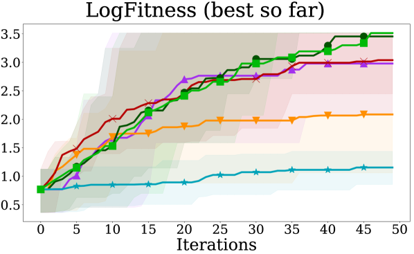
(a) Halogenase, $n=3$, $18$ reps.

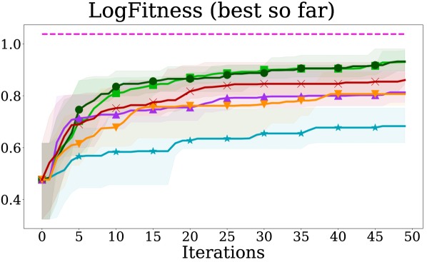
(b) GB1(4), $n=4$, $18$ reps.

(c) GFP, $n=6$, $10$ reps.

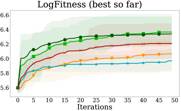
(d) GFP, $n=8$, $10$ reps.

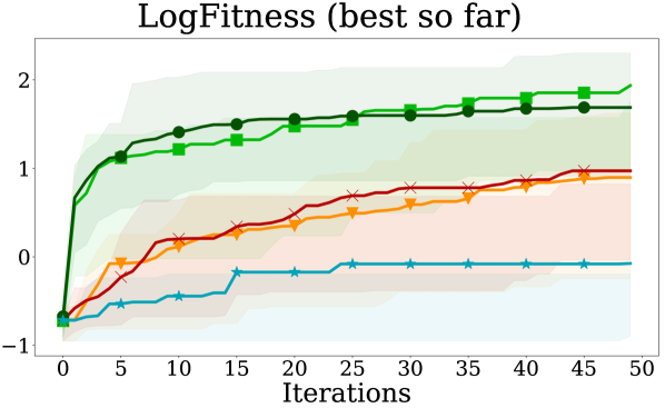
(e) GB1(55), $n=10$, $10$ reps.

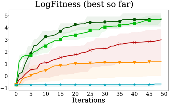
(f) GB1(55), $n=55$, $10$ reps.

Figure 2: Convergence speed of methods in terms of log fitness value of the best-so-far protein across BO iterations, under batch size $B=5$. Results are averaged over replications initiated with different training sets: $100$ protein variants for Halogenase and GB1(4), and $1000$ protein variants for other domains. Error bars are interquartile ranges averaged over replications. In all experiments GameOpt with Ibr and Hedge subroutines discover better protein sequences at a much faster rate.

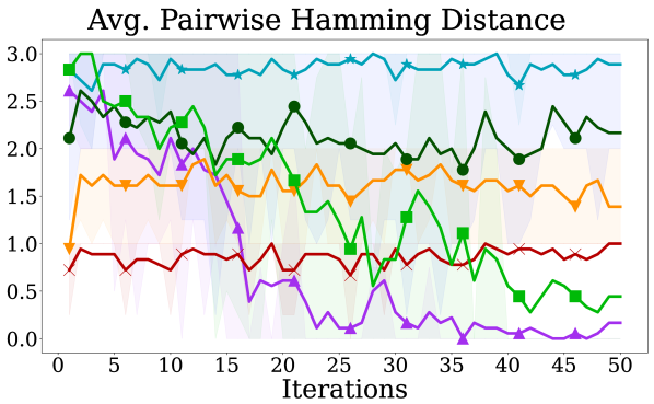
(a) Halogenase, $n=3$, $18$ reps.

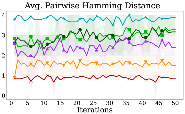
(b) GB1(4), $n=4$, $18$ reps.

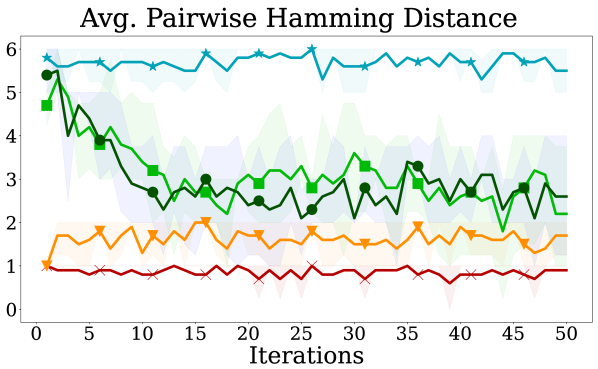
(c) GFP, $n=6$, $10$ reps.

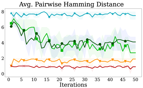
(d) GFP, $n=8$, $10$ reps.

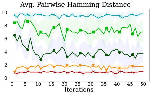
(e) GB1(55), $n=10$, $10$ reps.

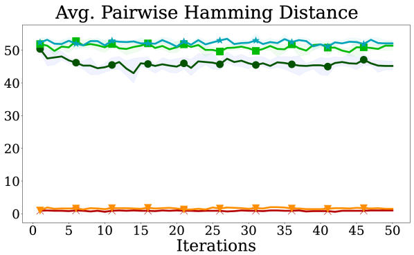
(f) GB1(55), $n=55$, $10$ reps.

Figure 3: Sampled batch diversity relative to past, measured via mean Hamming distance between executed and proposed variants from the previous iteration (pairwise distance), under batch size $B=5$. Results are averaged over replications initiated with different training sets: $100$ protein variants for Halogenase and GB1(4), and $1000$ protein variants for other domains. Error bars show interquartile ranges averaged over replications. In all experiments GameOpt consistently samples a rather diverse batch of evaluation points w.r.t. past proposed variants. This enhanced exploration of the search space contributes to its strong performance compared to the baseline methods.

5.4 Results

GameOpt variants, with Ibr and Hedge equilibrium computation subroutines, consistently outperform baselines across all experiments, discovering higher fitness protein sequences faster (see Figure 2).

Results for Halogenase. While initially surpassed by IBR-Fitness, PR, and GP-UCB, GameOpt variants converge faster to higher log fitness proteins than baselines. Notably, IBR-Fitness performs best-responses on the true log fitness function, whereas GameOpt-Ibr simulates best-response dynamics directly on the UCB model, allowing to compute equilibria at each iteration. Additionally, although GP-UCB performs comparably, it incurs higher computational demands. Furthermore, PR and Random perform poorly in the Halogenase setting.

Results for GB1(4). Similarly, GameOpt approaches steadily surpass PR and GP-UCB while exploring superior protein sequences efficiently. Initially trailing IBR-Fitness, GameOpt approaches prove more adept at exploring and sampling diverse points over iterations (see Figure 4 in Appendix E).

The baseline PR is not very competitive and also comes with higher computational demands. As highlighted in Section 3.2, PR relies on the expected UCB as the acquisition function, requiring expectation computation across players set and amino acid choices. This makes its performance contingent on accurately estimating expected UCB through combinatorially many sequence samples. In contrast, GameOpt efficiently finds stable outcomes by breaking down the combinatorial search space into individual decision sets, resulting in a more manageable process.

Finally, of particular observation is the subpar performance of GP-UCB and Random. A detailed analysis of GP-UCB’s performance is presented in Appendix E.5, where it is observed that the efficacy of GP-UCB heavily relies on the quality of the initial GP surrogate. In contrast, GameOpt demonstrates robustness in overcoming the limitations of a model initialized with a limited amount of data, thereby enhancing its sample efficiency. Further discussion on the performance of methods can be found in Appendix E.

Results for GFP. The complexity of the problem positively correlates with the performance gap between GameOpt and baselines. In the protein search space with $6$ and $8$ amino acid decisions, GameOpt with either subroutine excels in identifying high-log fitness protein sequences even from the start. Figure 3 further demonstrates GameOpt’s consistent exploration of diverse batches and Figure 4 in Appendix E shows its high rate of exploration.

Results for GB1(55). In both versions of the most complex problem domain, GameOpt demonstrates superior performance. As the decision flexibility (i.e., the number of players) increases from $10$ to $55$, the performance gap against baselines widens. Furthermore, GameOpt achieves incomparable batch diversity concerning past, both with respect to the initial training and previously executed protein sequences, as shown in Figures 3 and  4 in Appendix E.

5.5 Further discussion and limitations

In our experiments, we compare to IBR-Fitness, which simulates currently employed strategies in the iterative protein optimization literature. This is by no means the only methodology applied in this field, and a comprehensive comparison is beyond the scope of this work. Similarly, in our experiments, we use batch size $B=5$. While we acknowledge this is a restrictive setup given the technological needs of common screenings, nevertheless, our results should be transferable and applicable irrespective of the batch size which differs to each laboratory setting.

6 Conclusions

We introduced GameOpt, a novel tractable game-theoretical approach to combinatorial BO that leverages game equilibria of a cooperative game between discrete inputs of a costly-to-evaluate black-box function to tractably optimize the acquisition function over combinatorial and unstructured spaces, and select informative points. Empirical analysis on challenging protein design problems showed that GameOpt surpassed baselines in terms of convergence speed, consistently identifying better protein variants more quickly, thereby being more resource-efficient. GameOpt is a versatile framework, allowing for exploration with different acquisition functions or mixed equilibrium concepts. As for future work, an adaptive grouping of players and employing joint strategies should be further investigated.

Societal impact statement

Protein engineering presents vast opportunities, including advancements in healthcare, biotechnology, and environmental sustainability. However, it also entails inherent risks, such as the inadvertent creation of pathogens or other unintended consequences. While our focus in this paper is primarily on the technical aspects of our work, we remain cognizant of the ethical, safety, and regulatory considerations that accompany protein design research.

Appendix

We gather here the technical proofs, the details on GameOpt’s application to protein design, and additional experiment results complementing the main paper.

Appendix A Proof of Theorem 4.2

The proof relies on the main confidence lemma (Srinivas et al.,, 2009, Lemma 5.1) which states that, when the confidence width is set as $\beta_{t}=2n\log\left(\sup_{i\in[n]}|\mathcal{X}_{i}|\frac{t^{2}\pi^{2}}{6\delta}\right)\geq 2\log\left(|\prod_{i=1}^{n}\mathcal{X}_{i}|\frac{t^{2}\pi^{2}}{6\delta}\right)$, then with probability at least $(1-\delta)$,

$$\mu_{t}(x)-\beta_{t}\sigma_{t}(x)\leq f(x)\leq\mu_{t}(x)+\beta_{t}\sigma_{t}(x),\quad\forall x\in\mathcal{X},\quad\forall t\geq 1.$$ (5)

In other words, $\text{UCB}(\mathcal{GP}^{t},\cdot)$ and $\text{LCB}(\mathcal{GP}^{t},\cdot)$ are upper and lower bound functions with high probability. For simplicity, we will use the notation $\text{UCB}_{t}(\cdot)$ and $\text{LCB}_{t}(\cdot)$ for $\text{UCB}(\mathcal{GP}^{t},\cdot)$ and $\text{LCB}(\mathcal{GP}^{t},\cdot)$, respectively.

Next, we show that after $T$ iterations the strategy reported by GameOpt: $x_{T^{\star}}$, with $T^{\star}=\arg\min_{t\in[T]}\max_{i,x^{i}}\text{UCB}_{t}(x^{i},x^{-i}_{t})-\text{LCB}_{t}(x_{t})$, is a $\epsilon_{T}$-approximate Nash equilibrium of $f$ with $\epsilon_{T}\leq\mathcal{O}(T^{-0.5}\sqrt{\gamma_{T}})$. The theorem statement then follows by a simple inversion of the aforementioned bound.

By definition, $x_{T^{\star}}$ is a $\epsilon_{T}$-approximate Nash equilibrium of $f$ when $\epsilon_{T}=\max_{i,x^{i}}f(x^{i},x_{T^{\star}}^{-i})-f(x_{T^{\star}})$, i.e. $\epsilon_{T}$ upper bounds all possible single-player deviations. We can bound the worst-case single-player deviation with probability $(1-\delta)$ by the following chain of inequalities:

$$\epsilon_{T}=\max_{i,x^{i}}f(x^{i},x_{T^{\star}}^{-i})-f(x_{T^{\star}}) \leq\max_{i,x^{i}}\text{UCB}_{T^{\star}}(x^{i},x_{T^{\star}}^{-i})-\text{LCB}_{T^{\star}}(x_{T^{\star}})$$ (6)

$$\leq\frac{1}{T}\sum_{t=1}^{T}\max_{i,x^{i}}\text{UCB}_{t}(x^{i},x^{-i}_{t})-\text{LCB}_{t}(x_{t})$$ (7)

$$=\frac{1}{T}\sum_{t=1}^{T}\max_{i,x^{i}}\text{UCB}_{t}(x^{i},x^{-i}_{t})-\text{UCB}_{t}(x_{t})+\frac{2}{T}\sum_{t=1}^{T}\beta_{t}\sigma_{t}(x_{t})$$ (8)

$$\leq\frac{2}{T}\sum_{t=1}^{T}\beta_{t}\sigma_{t}(x_{t})\leq\mathcal{O}(T^{-0.5}\sqrt{\beta_{T}\gamma_{T}}).$$ (9)

The first inequality follows from the confidence lemma (5). The second one, by the fact that $\max_{i,x^{i}}\text{UCB}_{T^{\star}}(x^{i},x_{T^{\star}}^{-i})-\text{LCB}_{T^{\star}}(x_{T^{\star}})\leq\max_{i,x^{i}}\text{UCB}_{t}(x^{i},x^{-i}_{t})-\text{LCB}_{t}(x_{t}),\forall t$, by definition of $T^{\star}$. The last inequality holds because, at each iteration $t$, $x_{t}$ is an equilibrium of the $\text{UCB}_{t}$ function. Finally, the last inequality is from (Srinivas et al.,, 2009, Lemma 5.4). ∎

Appendix B GameOpt for Protein Design

The core concept of the GameOpt framework is inspired by the principles of natural evolution. In protein design, achieving equilibrium of a cooperative game over protein sites mirrors the iterative mutation and selection process in evolution. Where it converges to beneficial mutant sequences, can be thought of as equilibrium of the game. Given that protein search spaces align well with the domain GameOpt works on, we introduce a specialized version of GameOpt, tailored for protein design applications.

Algorithm 4 GameOpt-Ibr for Protein Design

1:  Input: GP prior $\mathcal{GP}^{0}(\mu_{0},k(\cdot,\cdot))$, initial data $\mathcal{D}_{0}=\{(x_{i},y_{i}=f(x_{i})+\epsilon)\}$, protein sites $\mathcal{N}$, batch size $B\in\mathbb{N}$, $M\in\mathbb{N}>B$, parameter $\beta$.

2:  for iteration $t=1,2,\dots,T$ do

3:     Construct game with reward function $\text{UCB}(\mathcal{GP}^{t-1},\beta,\cdot):\prod_{i=1}^{n}\mathcal{X}^{(i)}\to\mathbb{R}$

4:     for $m=1,2,\dots,M$ do

5:        $x^{br}_{0}\leftarrow$ random starting protein sequence, $x^{br}_{0}\in\mathcal{X}$

6:        for round $k=1,2,\dots,K$ do  */ BR game

7:           $\mathcal{X}^{br}_{k}\leftarrow\Big{\{}(x^{i,br},x_{k-1}^{-i,br}),\text{ such that }x^{i,br}=\arg\max_{x\in\mathcal{X}^{(i)}}\text{UCB}(x,x_{k-1}^{-i,br})\Big{\}}_{i=1}^{n}$

8:           Play $x^{br}_{k}\leftarrow\arg\max_{\boldsymbol{x}_{k}\in\mathcal{X}^{br}_{k}}[\text{UCB}(x_{k})]$

9:        end for

10:        Collect equilibrium protein sequence $x_{t,m}\leftarrow x^{br}_{K}$

11:     end for

12:     Select batch of top $B$ equilibrium protein sequences $\{x_{t,i}\}_{i=1}^{B}$ according to $\text{UCB}(\mathcal{GP}^{t-1},\beta,\cdot)$. */ Filtering

13:     Obtain fitness evaluations $y_{t,i}=f(x_{t,i})+\epsilon_{t,i},\quad\forall i=1,\ldots,B$

14:     Update $\mathcal{D}_{t}\leftarrow\mathcal{D}_{t-1}\cup\{(x_{t,i},y_{t,i})\}_{i=1}^{B}$

15:     Posterior update of model $\mathcal{GP}^{t}$ with $\mathcal{D}_{t}$

16:  end for

Algorithm 5 GameOpt-Hedge for Protein Design

1:  Input: GP prior $\mathcal{GP}^{0}(\mu_{0},k(\cdot,\cdot))$, initial data $\mathcal{D}_{0}=\{(x_{i},y_{i}=f(x_{i})+\epsilon)\}$, protein sites $\mathcal{N}$, batch size $B\in\mathbb{N}$, $M\in\mathbb{N}>B$, parameters $\beta,\eta$.

2:  for iteration $t=1,2,\dots,T$ do

3:     Construct game with reward function $\text{UCB}(\mathcal{GP}^{t-1},\beta,\cdot):\prod_{i=1}^{n}\mathcal{X}^{(i)}\to\mathbb{R}$

4:     for $m=1,2,\dots,M$ do

5:        Initialize weights $\boldsymbol{w}_{1}\leftarrow\frac{1}{W}[1,\dots,1]\in\mathbb{R}^{\mid\mathcal{N}\mid\times W}$

6:        for round $k=1,2,\dots,K$ do  */ Simultaneous Hedge

7:           Sample $x^{i}_{k}\sim\boldsymbol{w}^{i}_{1},\forall i\in\mathcal{N}$

8:           Set joint strategy $x_{k}\leftarrow\bigcup_{i\in\mathcal{N}}x^{i}_{k}$

9:           for player $i\in\mathcal{N}$ do  */ Players’ payoff

10:              $\ell_{x^{-i}_{k}}\leftarrow[v(x^{j,-i}_{k})]_{\forall j\in\mathcal{X}^{(i)}}$, where
$x^{j,-i}_{k}={j}\cup\{\bigcup_{i^{\prime}\in\mathcal{N}\setminus\{i\}}x^{i^{\prime}}_{k}\},\forall j\in\mathcal{X}^{(i)}$

11:              Set $\boldsymbol{w}^{i}_{k+1}\propto\boldsymbol{w}^{i}_{k}\text{ exp}(\eta\ell_{x^{-i}_{k}})$

12:           end for

13:        end for

14:        Collect equilibrium protein sequence $x_{t,m}\leftarrow x_{K}$

15:     end for

16:     Select batch of top $B$ equilibrium protein sequences $\{x_{t,i}\}_{i=1}^{B}$ according to $\text{UCB}(\mathcal{GP}^{t-1},\beta,\cdot)$. */ Filtering

17:     Obtain fitness evaluations $y_{t,i}=f(x_{t,i})+\epsilon_{t,i},\quad\forall i=1,\ldots,B$

18:     Update $\mathcal{D}_{t}\leftarrow\mathcal{D}_{t-1}\cup\{(x_{t,i},y_{t,i})\}_{i=1}^{B}$

19:     Posterior update of model $\mathcal{GP}^{t}$ with $\mathcal{D}_{t}$

20:  end for

Appendix C Baselines

In Section 5, we empirically evaluate GameOpt against existing baselines which we detail next. These include IBR-Fitness, inspired by directed evolution (Algorithm 6), Random (Algorithm 7), which samples evaluation points randomly, and PR, an optimizer of expected UCB (Daulton et al.,, 2022). We further compared GameOpt with discrete local search methods in E.2.

Algorithm 6 Iterative Best Response-Fitness (Ibr-Fitness)

1:  Input: Domain $\mathcal{X}$, fitness function $f:\mathcal{X}\to\mathbb{R}$, players $\mathcal{N}$, initial data $\mathcal{D}_{0}=\{(x_{i},y_{i}=f(x_{i})+\epsilon)\}$, batch size $B\in\mathbb{N}$.

2:  $x^{br}_{0}\leftarrow$ random joint strategy, $x^{br}_{0}\in\mathcal{X}$

3:  for iteration $t=1,2,\dots,T$ do

4:     Randomly selected $B$ players $\in\mathcal{N}$ generates BRs $\{x_{t,i}\}_{i=1}^{B}$ w.r.t. $x^{br}_{t-1}$ based on $f(\cdot)$

5:     Obtain evaluations $y_{t,i}=f(x_{t,i})+\epsilon_{t,i},\quad\forall i=1,\ldots,B$

6:     Update $\mathcal{D}_{t}\leftarrow\mathcal{D}_{t-1}\cup\{(x_{t,i},y_{t,i})\}_{i=1}^{B}$

7:     Play $x^{br}_{t}\leftarrow\arg\max_{x_{t,i}\in\{x_{t,i}\}_{i=1}^{B}}y_{t,i}$

8:  end for

9:  return $x^{\star}_{T}\leftarrow\arg\max_{(x,y)\in\mathcal{D}_{T}}y$ */ Best-so-far

Algorithm 7 Random

1:  Input: Domain $\mathcal{X}$, $f:\mathcal{X}\to\mathbb{R}$, initial data $\mathcal{D}_{0}=\{(x_{i},y_{i}=f(x_{i})+\epsilon)\}$, batch size $B\in\mathbb{N}$.

2:  for iteration $t=1,2,\dots,T$ do

3:     Randomly generate batch of $B$ points $\{x_{t,i}\}_{i=1}^{B},\forall x_{t,i}\in\mathcal{X}$

4:     Obtain evaluations $y_{t,i}=f(x_{t,i})+\epsilon_{t,i},\quad\forall i=1,\ldots,B$

5:     Update $\mathcal{D}_{t}\leftarrow\mathcal{D}_{t-1}\cup\{(x_{t,i},y_{t,i})\}_{i=1}^{B}$

6:  end for

7:  return $x^{\star}_{T}\leftarrow\arg\max_{(x,y)\in\mathcal{D}_{T}}y$ */ Best-so-far

Appendix D Experiment details

We set the (hyper)parameters for the experiments as in Table 1.

Table 1: (Hyper) parameter values.

(Hyper) parameter	Explanation	Value
$T$	The number of active learning (BO) iterations	$50$
$K$	The number of game rounds	$40$ for GFP, $200$ for Halogenase and GB1(55), and $400$ for GB1(4);
		$50$ for GameOpt-Ibr in GB1(55) & $n=10$ domain
		$100$ for GameOpt-Ibr in GB1(55) & $n=55$ domain
$n=\mid\mathcal{N}\mid$	The number of players	$3$ for Halogenase, $4$ for GB1(4), $6$ and $8$ for GFP, $10$ and $55$ for GB1(55)
$\mid\mathcal{D}_{0}\mid$	The number of samples in training set	$100$ for Halogenase and GB1(4), and $1000$ for GFP and GB1(55)
$\eta$	Learning rate	$0.5$ under Halogenase and $2.0$ for the rest of the problem settings
$\epsilon$	Observation noise for each training example	$0.0004$
$l$	RBF kernel lengthscale	optimized offline
$\beta$	The UCB tuning parameter	$2$
$B$	Batch size per BO iteration	5

GB1(4)

The dataset (Wu et al.,, 2016) is fully combinatorial, i.e., encompassing fitness measurements of $20^{4}$ variants with $4$ sites. In this context, each protein site is treated as a player in the cooperative game of GameOpt, with $\mathcal{N}=\{1,\dots,4\}$. Additionally, we also analyzed the effect of player grouping inspired by epistasis phenomenon in protein design and provided the analysis in Appendix E.

We train the GP surrogate by utilizing a small portion of the dataset, specifically $0.0625\%$, consisting of $100$ protein variants. Since existing literature does not provide common ground feature embeddings as representations for the GB1(4) variants, we use chemical descriptors (Wu et al.,, 2019) to extract $60$ feature embeddings using a training set of size $1000$ protein variants with LASSO method. We apply $k$-fold cross-validation with $k=18$ different train/test dataset partitions. Following this, we evaluate the performance of our approach over $18$ replications. In each replication, we initialize the GP surrogate-based baseline methods with the same initial GP model as our approach. We also use the same initial protein sequence for comparison within that replicate but employ different initial points across replications. We set the starting joint strategy as the protein sequence having the highest log fitness value in the training set. The prior mean of the GP is fixed at $1.0162$. For the kernel hyperparameters, $60$ lengthscales are defined for each feature dimension and optimized offline at the beginning of a replication; outputscale is set to $0.02169$.

GB1(55)

We experiment on the non-exhaustive dataset GB1(55) that only includes 2-point mutations throughout the entire $55$ residues of the GB1 protein resulting in $535,917$ variants (Olson et al.,, 2014) and consider two settings: $55$ and $10$ number of players.

GB1(55) with $\boldsymbol{55}$ Players

In this context, we treat each protein site as a player in the GameOpt, thus, $\mathcal{N}=\{1,\dots,55\}$.

As the dataset is not completely combinatorial, we do not have access to measured fitness values for all $20^{55}$ variants. To overcome this, we employ a Deep Neural Network-based (DNN) oracle to predict fitness scores using feature embeddings associated with the protein sequences. We again opt to feature embeddings as the representation for categorical input of GP surrogate. Unlike GB1(4), we utilize the ESM-1v protein language model from esm introduced by Meier et al., (2021), specifically designed for predicting protein variant effects and can be used to extract embeddings. With ESM-1v, we represent a sequence through a $1280$ dimensional feature embedding vector. We train the oracle with supervised learning, using the training set having $(477\,854\times 1280,477\,854)$ feature & label pairs. Obtaining the exhaustive version of the GB1(55) dataset, we train the GP surrogate using ESM-1v feature embeddings of $1000$ randomly generated protein variants and corresponding oracle-predicted fitness scores for $10$ replications.

GB1(55) with $\boldsymbol{10}$ players

To further analyze the performance of GameOpt compared to the other baselines, we consider the setting where among the $55$ sites, only $10$ most significant protein sites can be mutated.

We employ the same protein language model for embeddings and oracle to predict fitness scores. However, the choice of $10$ players among ${55\choose 10}$ possibilities is a strategic decision that affects the design performance. For this, we define the significance of a protein site considering the average variation in the fitness scores in the dataset. Concretely, we use Algorithm 8 and select $\mathcal{N}=\{21,24,35,39,41,45,46,47,48,50\}$ sites as the players. We treat the rest of the protein sequence, i.e., sites that do not correspond to players as fixed.

Algorithm 8 ComputeMostSignificantSites

1:  Input: Dataset $\mathcal{D}=(x_{i},y_{i})_{i=1}^{N}$, players $K$, protein sequence length $L$, amino acids set $\mathcal{A}$.

2:  Initialize $players\leftarrow\emptyset$, ${site\_score}^{k}_{a}\leftarrow\emptyset$ and ${site\_var}^{k}\leftarrow 0,\forall k\in\{1,\dots,L\},a\in\mathcal{A}$

3:  for each pair $(x_{i},y_{i})\in\mathcal{D}$ do

4:     for each site $k\in\{1,\dots,L\}$ do

5:        Set amino acid in site $k$ as $a\leftarrow x_{i}^{k}$

6:        Append ${site\_score}^{k}_{a}\leftarrow{site\_score}^{k}_{a}\cup\{y_{i}\}$

7:     end for

8:  end for

9:  ${site\_score}^{k}\leftarrow\bigcup_{a\in\mathcal{A}}{site\_score}^{k}_{a},\forall k\in\{1,\dots,L\}$

10:  ${site\_var}^{k}\leftarrow stdev({site\_score}^{k}),\forall k\in\{1,\dots,L\}$

11:  return $K$ sites having highest ${site\_score}$ as players

Halogenase

Halogenase is a non-exhaustive dataset involving fitness measurements for $605$ unique variants. To obtain the complete protein fitness landscape, we again construct an oracle, i.e., an MLP having $R^{2}=0.96$ on a test set and experiment on a setting where each protein site is a player.

GFP with $\boldsymbol{6}$ players

The Aequorea victoria green-fluorescent protein dataset only includes fitness measurements of $35,584$ variants corresponding to mixed mutations of some positions on a $238$ length sequence. For the fully combinatorial protein fitness landscape, we construct an oracle, i.e., an MLP with test $R^{2}=0.90$ and choose $6$ positions: $\mathcal{N}=\{10,18,22,37,67,78\}$ that have the largest number of mutations in the original dataset as the players of the GameOpt.

GFP with $\boldsymbol{8}$ players

To set the players in this setting, we identified $8$ positions that have the largest number of mutations in the original dataset: $\mathcal{N}=\{10,18,22,37,67,78,196,112\}$.

Appendix E Additional experimental results

E.1 Sample batch diversity

We also evaluate our method against baselines in terms of performance metric: sampled batch diversity concerning the past. It is measured via the mean Hamming distance of executed points at each BO iteration to the $(1)$ closest initial training point and $(2)$ the proposed point at the previous iteration (pairwise distance).

The results depicted in Figure 4 underscore that GameOpt explores at a faster rate compared to baselines except for Random. Notably, even in the initial iterations, GameOpt demonstrates the capability to discover points beyond the trust region of its GP prior. Furthermore, it consistently upholds the sampled batch diversity compared to previously executed strategies. As also illustrated in Figure 3, GameOpt explores effectively at the beginning and gradually converges to a region conducive to exploitation. This enhanced exploration across the search space contributes to its outperforming performance in identifying high fitness-valued protein sequences.

On the other hand, the exploration strategy employed by Random relies on the generation of $B$ best responses through random selection, a method that does not consistently ensure a diverse sampled batch in the input space. Furthermore, IBR-Fitness shows a moderate sampled batch diversity concerning the past, attributed to its more exploitative nature—specifically, the sampling of $B$ best responses based on true log fitness values in comparison to other baseline methods. While PR manages to maintain a diverse sampled batch concerning the past in the context of GB1(4), its performance falters when applied to other settings. Additionally, the sampling process of PR involves computing the expected UCB across all potential strategy combinations of players, making its performance, and consequently its sampled batch diversity, highly reliant on an accurate estimate of this expectation.

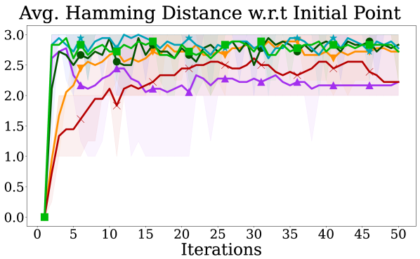
(a) Halogenase, $n=3$, $18$ reps.

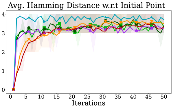
(b) GB1(4), $n=4$, $18$ reps.

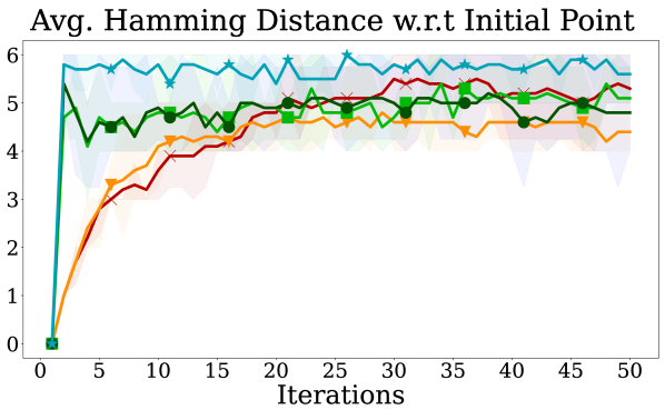
(c) GFP, $n=6$, $10$ reps.

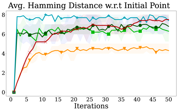
(d) GFP, $n=8$, $10$ reps.

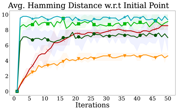
(e) GB1(55), $n=10$, $10$ reps.

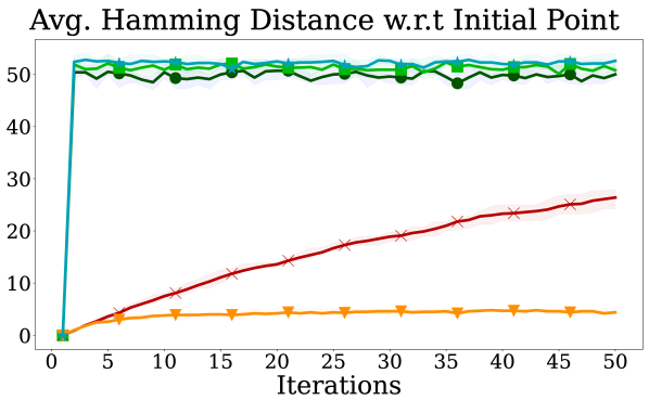
(f) GB1(55), $n=55$, $10$ reps.

Figure 4: Performance results for the sampled batch diversity w.r.t past measured via mean Hamming distance between the executed variant and the closest initial point from the training set, under batch size $B=5$. Each point on each line is the average of multiple replications initiated with different training sets having $100$ variants for GB1(4) & Halogenase and $1000$ for GB1(55) & GFP. Similarly, error bars are interquartile ranges averaged over replications. In all experiments, GameOpt explores significantly faster than the baseline methods.

E.2 Comparison with Discrete Local Search methods

We further compared GameOpt against Discrete Local Search baselines DLS and DLS_Best (Balandat et al.,, 2020) that perform a discrete local search by exploring k-Hamming distance neighborhood. While DLS employs random initialization, DLS_Best starts the local search from the best-discovered sequence. In our experiments, we set their neighborhood size as 2-Hamming distance and let the baselines greedily select $B$ sequences at each iteration. For a fair comparison against DLS_Best, we also run the best-discovered sequence initialization version of our approach, called GameOpt-Ibr_Best.

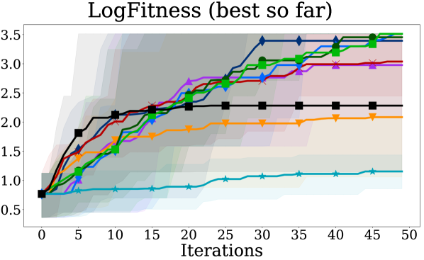
(a) Halogenase, $n=3$, $18$ reps.

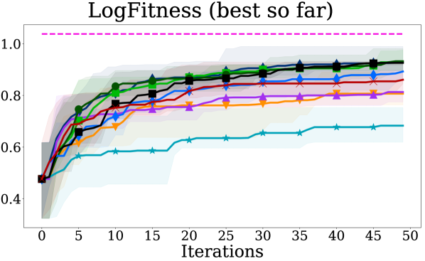
(b) GB1(4), $n=4$, $18$ reps.

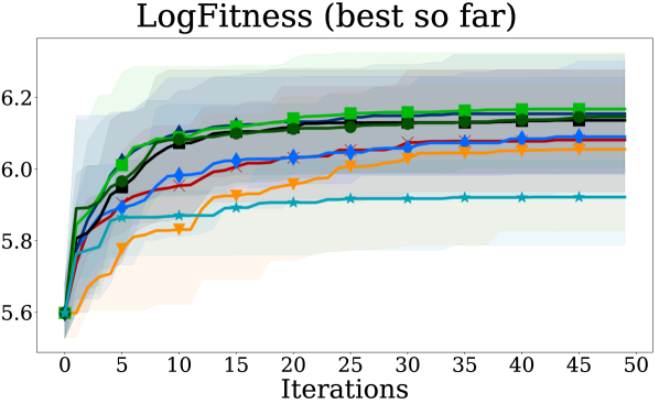
(c) GFP, $n=6$, $10$ reps.

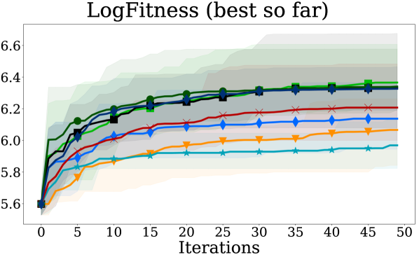
(d) GFP, $n=8$, $10$ reps.

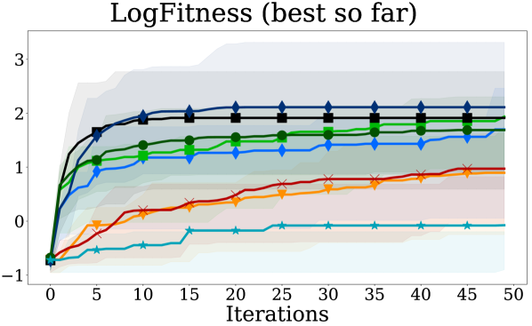
(e) GB1(55), $n=10$, $10$ reps.

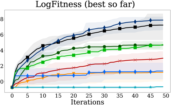
(f) GB1(55), $n=55$, $10$ reps.

Figure 6: Convergence speed of methods in terms of log fitness value of the best-so-far protein throughout BO iterations, under batch size $B=5$. Each point is the average of multiple replications initiated with different training sets having $100$ protein variants for Halogenase and GB1(4), and $1000$ protein variants for the rest of the problem domains. Similarly, error bars are interquartile ranges averaged over replications.

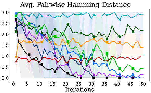
(a) Halogenase, $n=3$, $18$ reps.

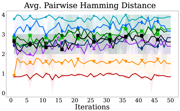
(b) GB1(4), $n=4$, $18$ reps.

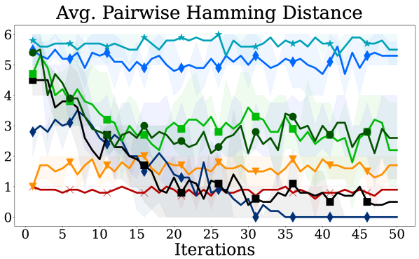
(c) GFP, $n=6$, $10$ reps.

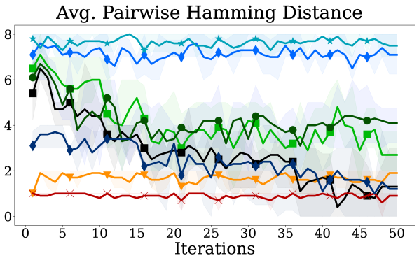
(d) GFP, $n=8$, $10$ reps.

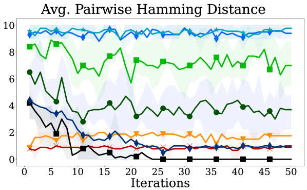
(e) GB1(55), $n=10$, $10$ reps.

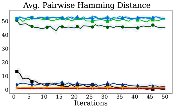
(f) GB1(55), $n=55$, $10$ reps.

Figure 7: Sampled batch diversity w.r.t past measured via mean Hamming distance between the executed variant and the proposed variant from the previous iteration (pairwise distance), under batch size $B=5$. Each point on each line is the average of multiple replications initiated with different training sets having $100$ variants for GB1(4) & Halogenase and $1000$ for GB1(55) & GFP. Similarly, error bars are interquartile ranges averaged over replications. In all experiments GameOpt consistently samples a rather diverse batch of evaluation points w.r.t. past proposed variants. This enhanced exploration of the search space contributes to its strong performance compared to the baseline methods.

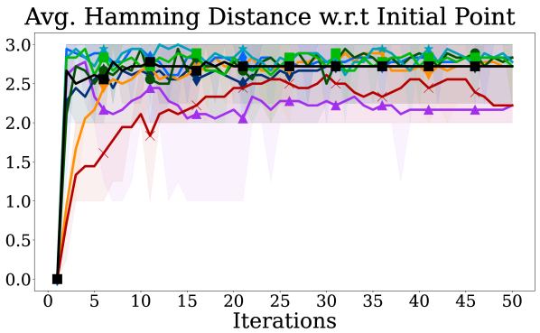
(a) Halogenase, $n=3$, $18$ reps.

(b) GB1(4), $n=4$, $18$ reps.

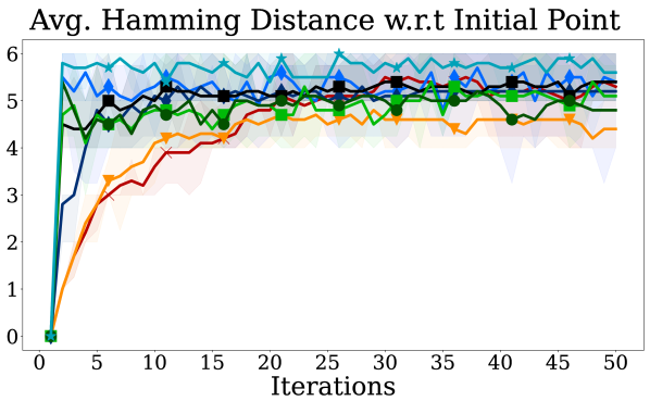
(c) GFP, $n=6$, $10$ reps.

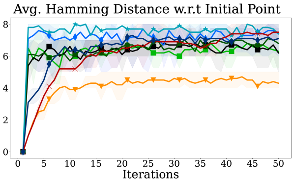
(d) GFP, $n=8$, $10$ reps.

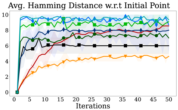
(e) GB1(55), $n=10$, $10$ reps.

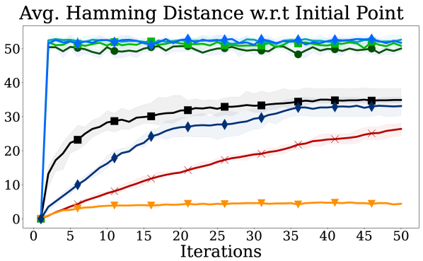
(f) GB1(55), $n=55$, $10$ reps.

Figure 8: Performance results for the sampled batch diversity w.r.t past measured via mean Hamming distance between the executed variant and the closest initial point from the training set, under batch size $B=5$. Each point on each line is the average of multiple replications initiated with different training sets having $100$ variants for GB1(4) & Halogenase and $1000$ for GB1(55) & GFP. Similarly, error bars are interquartile ranges averaged over replications. In all experiments, GameOpt explores faster than the baseline methods, except for Random and DLS.

We remark that DLS and DLS_Best can be seen as constrained versions of GameOpt that require a prior definition of the neighborhood (thus, unlike our approach, they require a notion of distance too). Moreover, being centralized, they are subject to a higher computational complexity which grows exponentially with the neighborhood size. For a sequence of length $n$ (players) with $\mid\mathcal{X}^{(i)}\mid=d$ many amino acid choices, GameOpt reduces the intractable optimization of acquisition function (i.e., $O(d^{n})$) to $O(nd)$ complexity. Instead, DLS & DLS_Best search over $k$-distance neighborhoods yielding $O(C(n,k)d^{k})$ complexity, where $C$ denotes the combination operation and $k$ is the Hamming distance. We observe GameOpt performs comparably to DLS baselines (see Figures 6, 8, 7, and additional analyses below), but requiring a significantly lower compute cost, as shown in Section E.3.

E.3 Computational costs

We report the total compute amount (measured in hours) for the experiments with $T=50$ BO iterations in Table 2. We conduct the experiments on an internal compute cluster equipped with NVIDIA A100 80 GB tensor-core GPUs. For smaller domains (with short protein sequences), we were able to execute replications concurrently without encountering memory errors. However, in configurations necessitating the generation of embeddings for numerous evaluation points with longer protein sequences in each iteration, parallel execution was not feasible, thus necessitating a per-replication computation time report. Specifically, we present the total compute amount for all replications across domains Halogenase, GB1(4), and GFP; whereas we report per replication compute amount accompanied by its standard deviation for the two largest GB1(55) domains.

Referring to Table 2, GameOpt variations provide tractable acquisition function optimization. Their computational demand predominantly hinges on the number of sequences they evaluate per BO iteration. This is also influenced by the number of game rounds–which we intentionally set to a higher value to guarantee convergence to game equilibrium (see Table 1 for the exact values). Nevertheless, our observations reveal that game equilibrium is often reached well before the rounds are completed. Consequently, the computational times reported for GameOpt can be considered to be within the worst-case scenario.

Table 2: Total compute amount (in hours) required for experiments with $T=50$ BO iterations. Each entry with $\pm$ represents the average per-replication computation time, accompanied by their standard deviation, whereas the others show the total compute time for all replications. We run $18$ replications for Halogenase, GB1(4), and $10$ replications for the other domains. In all domains, particularly for the larger search spaces, GameOpt provides tractable acquisition function optimization.

Method	Domain
	Halogenase	GB1(4)	GFP, $n=6$	GFP, $n=8$	GB1(55), $n=10$	GB1(55), $n=55$
GameOpt-Ibr	$\mathbf{0.19}$	$\mathbf{0.30}$	$\mathbf{1.02}$	$\mathbf{2.74}$	$\mathbf{1.61\pm 0.46}$	$\mathbf{11.25\pm 3.19}$
GameOpt-Hedge	2.44	1.95	$2.05\pm 0.02$	$2.60\pm 0.09$	$3.85\pm 0.39$	$20.13\pm 1.04$
GP-UCB	0.63	29.56	-	-	-	-
DLS	0.29	1.10	$2.90\pm 0.33$	$4.94\pm 0.24$	$4.10\pm 2.36$	$102.86\pm 27.42$

E.4 Additional analyses

We performed further analyses to assess the effectiveness of our GameOpt framework against baselines in terms of: $(1)$ fraction of global optima discovered, $(2)$ fraction of solutions found above a fitness threshold, $(3)$ cumulative maximum for sequences proposed and $(4)$ mean pairwise Hamming distance between proposed sequences.

We evaluated the fraction of global optima discovered under the GB1(4) setting, as depicted in Table 3. For this fully combinatorial dataset, we identify the global optimizer sequence by exhaustive search. Our findings revealed that GameOpt-IBR successfully identified the global optimum sequence in $33.33\%$ of cases out of 18 replications, highlighting its superior convergence against baselines.

Additionally, given the difficulty of identifying global optima in non-fully combinatorial datasets, we examined the fraction of optima found above a fitness threshold, $f_{\tau}=0.8$. Table 4 demonstrates that across all problem domains (excluding best cumbersome initialization versions), the GameOpt framework consistently samples batches containing a higher number of optimal sequences compared to baseline methods. Its effectiveness is highlighted more as the search space size gets higher. In the most complex domain, GB1(55) with $55$ players, its best cumbersome initialization version performs comparably to DLS_Best. However, it is essential to also acknowledge the comparison w.r.t the computational complexity associated with that configuration as discussed in Appendix E.3.

Regarding the cumulative maximum for proposed sequences (see Table 5), our framework demonstrates notable performance by consistently proposing protein variants with higher fitness values. Moreover, its superior convergence speed, illustrated in Figure 6, underscores its effectiveness against baselines including DLS. The discrete local search with best initialization, DLS_Best, converges relatively slower, particularly in small domains, yet performs comparably against GameOpt_Best in finding high log fitness valued variants. However, it does not provide tractable optimization as detailed in Appendix E.3.

Furthermore, we analyzed the performance of methods considering the mean pairwise Hamming distance between the sequences proposed at each BO iteration (see Table 6 and Figure 7) which is an indicator for sampled batch diversity. The results indicate that GameOpt explores moderately, however, it balances exploration and exploitation to prevent over-exploring seen in Random and DLS, as well as over-exploiting observed in GameOpt_Best, DLS_Best and PR.

Lastly, the mean Hamming distance between the proposed variant and the closest initial point from the training set (see Figure 8) showcases that GameOpt explores the solution space faster than the baseline methods, except for Random and DLS.

Table 3: Fraction of global optima found for the $GB1(4)$ dataset. Each entry is the average of $18$ replications. GameOpt variations are able to sample global optimum sequence (AHCA) more frequently compared to other baselines. Entries of the outperforming methods are denoted in bold. The results show that GameOpt-IBR converges to the best strategy more frequently compared to the baselines.

Method	% best strategy (AHCA) found
GameOpt-Ibr	$\boldsymbol{33.33}$
GameOpt-Hedge	$16.67$
IBR-Fitness	$16.67$
PR	$0.00$
GP-UCB	$0.00$
Random	$0.00$
DLS	$0.00$
DLS_Best	$11.11$
GameOpt-Ibr_Best	$11.11$

Table 4: Percentage of computed candidates that are above a threshold of $f_{\tau}=0.8*$(maximum fitness value). Each entry is the average of $18$ replications for Halogenase and GB1(4) settings, and $10$ replications for the others. Entries of the outperforming methods are denoted in bold. Results indicate the effectiveness of GameOpt variations on sampling more optima than the baseline methods.

Method	Domain
	Halogenase	GB1(4)	GFP, $n=6$	GFP, $n=8$	GB1(55), $n=10$	GB1(55), $n=55$
GameOpt-Ibr	$\boldsymbol{100.00}$	$\boldsymbol{21.20}$	$\boldsymbol{28.52}$	50.96	11.60	1.96
GameOpt-Hedge	94.44	14.62	26.68	$\boldsymbol{61.72}$	9.48	2.12
IBR-Fitness	72.22	7.46	18.96	35.32	0.36	0.00
PR	38.89	2.05	15.96	15.32	0.00	0.04
GP-UCB	72.22	4.82	-	-	-	-
Random	0.00	0.29	0.76	1.60	0.00	0.00
DLS	94.44	7.46	22.60	36.48	0.16	0.00
DLS_Best	88.89	19.88	16.80	45.92	2.64	52.24
GameOpt-Ibr_Best	44.44	17.40	12.32	42.64	1.68	48.64

Table 5: Cumulative maximum for sequences proposed at the end of the BO iterations. Each entry is the average of $18$ replications for Halogenase and GB1(4) settings, and $10$ replications for the others. Entries of the outperforming methods are denoted in bold. GameOpt variations show superior performance in proposing higher fitness-valued protein variants.

Method	Domain
	Halogenase	GB1(4)	GFP, $n=6$	GFP, $n=8$	GB1(55), $n=10$	GB1(55), $n=55$
GameOpt-Ibr	3.51	0.93	6.17	6.37	1.94	4.72
GameOpt-Hedge	3.45	0.94	6.15	6.34	1.69	4.66
IBR-Fitness	3.10	0.86	6.08	6.21	0.97	2.99
PR	2.08	0.81	6.06	6.07	0.90	1.18
GP-UCB	2.98	0.82	-	-	-	-
Random	1.15	0.68	5.92	5.97	-0.08	-0.66
DLS	3.51	0.89	6.09	6.14	1.70	1.35
DLS_Best	3.40	0.93	6.15	6.33	2.11	7.87
GameOpt-IBR_Best	2.28	0.93	6.14	6.33	1.91	7.25

Table 6: Mean pairwise Hamming distance between the sequences proposed at each iteration. Each entry is the average of $18$ replications for Halogenase and GB1(4) settings, and $10$ replications for the others. In all problem domains, Random baseline consistently samples a rather diverse batch of evaluation points w.r.t. past proposed variants. Although this shows enhanced exploration, one drawback is the lack of exploitation. Hence, as illustrated in Figure 3, GameOpt balances these two successfully and shows a moderate sampled batch diversity.

Method	Domain
	Halogenase	GB1(4)	GFP, $n=6$	GFP, $n=8$	GB1(55), $n=10$	GB1(55), $n=55$
GameOpt-Ibr	1.40	2.94	3.08	4.11	7.32	50.93
GameOpt-Hedge	2.13	2.91	2.93	4.23	3.98	45.89
IBR-Fitness	0.86	0.88	0.85	0.89	0.86	0.89
PR	1.61	1.57	1.61	1.67	1.69	1.60
GP-UCB	0.77	2.41	-	-	-	-
Random	2.85	3.8	5.69	7.64	9.51	52.34
DLS	1.13	3.36	5.13	7.13	9.38	52.19
DLS_Best	0.68	2.56	1.18	2.36	1.55	3.57
GameOpt-IBR_Best	0.33	2.64	1.48	2.78	0.57	3.12

E.5 Comparison with GP-UCB

We further analyzed the saturating behavior exhibited by GP-UCB in the GB1(4) setting. As depicted in Figure 5, our investigation focused on the influence of the initial GP surrogate model, considering different training set sizes, specifically with $100$ and $500$ training points.

Our findings underscore that the efficacy of GP-UCB heavily relies on the quality of the initial GP surrogate model. Particularly, an initial GP surrogate trained with only $100$ data points proves insufficient for GP-UCB to effectively identify high-log fitness protein sequences. Given that GP-UCB optimizes the UCB globally and selects the $B$ best points in each iteration, the limited informativeness of sampled batch points under this GP surrogate constrains the algorithm. Therefore, GP-UCB ends up converging to a point where further improvement is impeded. In contrast, employing a potentially more informative GP model with $500$ training points enables GP-UCB to perform comparably to GameOpt. Our proposed approach, however, exhibits robustness by overcoming the constraints associated with a model initialized with limited data. Through computing evaluation points as the equilibria of cooperative game-playing, it consistently gathers diverse and informative batches to guide the GP, thereby enhancing sample efficiency.

(a) $100$ training points.

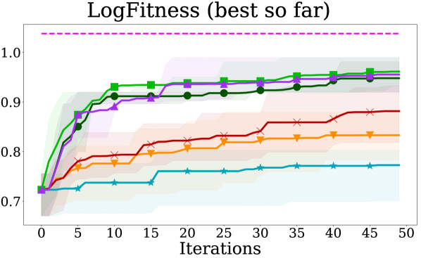
(b) $500$ training points.

Figure 5: The effect of training set size on the performance under setting GB1(4), $n=4$, $18$ reps. GP-UCB mitigates saturating behavior when leveraging a more informative initial GP surrogate model. In contrast, GameOpt showcases resilience in overcoming the limitations associated with a GP model trained with a limited amount of data.

E.6 Exploring Players’ Grouping

Until this juncture, we have exclusively examined scenarios where a GameOpt player is responsible for only a single site within the protein sequence. In light of the epistasis (Phillips,, 2008) phenomenon in protein design, which underscores how the effect of a mutation on fitness can be influenced by the presence of other mutations within the same protein, we now explore the concept of grouping protein sites together, i.e., having players being responsible for more than one site. This is because modeling protein sites independently may yield different fitness outcomes than finding equilibria among groups of several sites. To this end, we conduct a preliminary investigation into whether this phenomenon alters GameOpt’s performance.

We experiment on GB1(4) with $\{0,1,2,3\}$ protein sites and $\mathcal{N}=\{1,2\}$ players, considering 3 possible player & site groupings: $\{(01,23),(02,13),(03,12)\}$. For instance, setting $(01,23)$ means that the first player is responsible for sites $\{0,1\}$ and the other one for $\{2,3\}$.

Our evaluations with GameOpt-Ibr and GameOpt-Hedge using the same performance measures (Figures 9 and  10) showed that there is no significant performance difference between individual players and grouping settings as they all discover the high log fitness valued protein variants at a similar rate while collecting batches of diverse evaluation points. Nevertheless, an in-depth examination of this phenomenon on larger datasets remains a subject for future investigation.

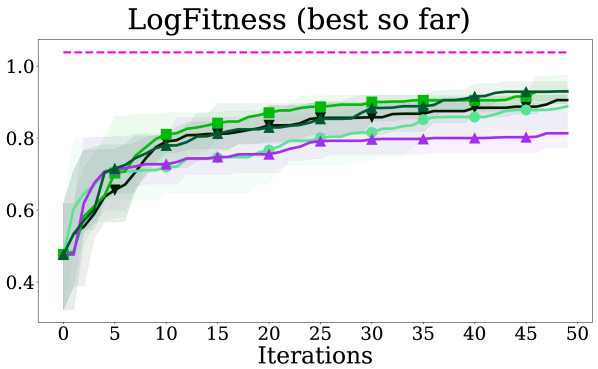
(a) Convergence speed

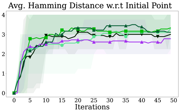
(b) Sample diversity w.r.t $(1)$

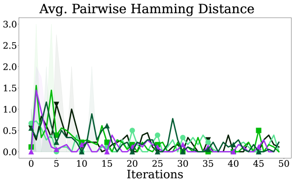
(c) Sample diversity w.r.t $(2)$

Figure 9: GameOpt-Ibr performance for player grouping, under GB1(4) setting, $18$ reps. There is no significant performance difference between individual players and player grouping settings under this domain.

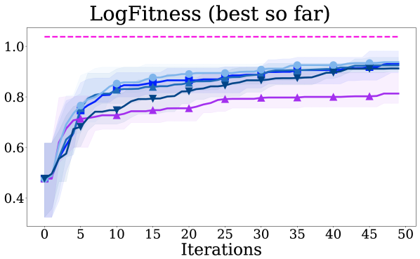
(a) Convergence speed

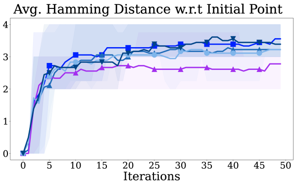
(b) Sample diversity w.r.t $(1)$

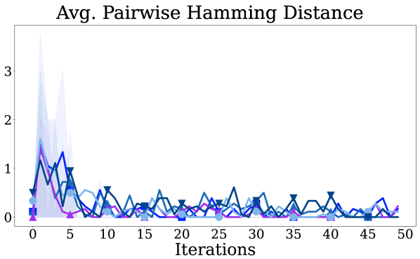
(c) Sample diversity w.r.t $(2)$

Figure 10: GameOpt-Hedge performance for player grouping, under GB1(4) setting, $18$ reps. No significant performance difference exists between individual players and player grouping settings under this domain.

References

- Angermueller et al., (2020) Angermueller, C., Belanger, D., Gane, A., Mariet, Z., Dohan, D., Murphy, K., Colwell, L., and Sculley, D. (2020). Population-based black-box optimization for biological sequence design. In International conference on machine learning, pages 324–334. PMLR.
- Arnold, (1998) Arnold, F. H. (1998). Design by directed evolution. Accounts of chemical research, 31(3):125–131.
- Balandat et al., (2020) Balandat, M., Karrer, B., Jiang, D. R., Daulton, S., Letham, B., Wilson, A. G., and Bakshy, E. (2020). BoTorch: A Framework for Efficient Monte-Carlo Bayesian Optimization. In Advances in Neural Information Processing Systems 33.
- Baptista and Poloczek, (2018) Baptista, R. and Poloczek, M. (2018). Bayesian optimization of combinatorial structures. In International Conference on Machine Learning, pages 462–471. PMLR.
- Biswas et al., (2021) Biswas, S., Khimulya, G., Alley, E. C., Esvelt, K. M., and Church, G. M. (2021). Low-n protein engineering with data-efficient deep learning. Nature methods, 18(4):389–396.
- Büchler et al., (2022) Büchler, J., Malca, S. H., Patsch, D., Voss, M., Turner, N. J., Bornscheuer, U. T., Allemann, O., Le Chapelain, C., Lumbroso, A., Loiseleur, O., et al. (2022). Algorithm-aided engineering of aliphatic halogenase welo5* for the asymmetric late-stage functionalization of soraphens. Nature Communications, 13(1):371.
- Cesa-Bianchi and Lugosi, (2006) Cesa-Bianchi, N. and Lugosi, G. (2006). Prediction, Learning, and Games. Cambridge University Press.
- Cheng et al., (2022) Cheng, L., Yang, Z., Hsieh, C., Liao, B., and Zhang, S. (2022). Odbo: Bayesian optimization with search space prescreening for directed protein evolution. arXiv preprint arXiv:2205.09548.
- Christodoulou and Koutsoupias, (2005) Christodoulou, G. and Koutsoupias, E. (2005). On the price of anarchy and stability of correlated equilibria of linear congestion games,,. In Brodal, G. S. and Leonardi, S., editors, Algorithms – ESA 2005.
- Dadkhahi et al., (2020) Dadkhahi, H., Shanmugam, K., Rios, J., Das, P., Hoffman, S. C., Loeffler, T. D., and Sankaranarayanan, S. (2020). Combinatorial black-box optimization with expert advice. In Proceedings of the 26th ACM SIGKDD International Conference on Knowledge Discovery & Data Mining, pages 1918–1927.
- Daulton et al., (2022) Daulton, S., Wan, X., Eriksson, D., Balandat, M., Osborne, M. A., and Bakshy, E. (2022). Bayesian optimization over discrete and mixed spaces via probabilistic reparameterization. Advances in Neural Information Processing Systems, 35:12760–12774.
- Deshwal et al., (2023) Deshwal, A., Ament, S., Balandat, M., Bakshy, E., Doppa, J. R., and Eriksson, D. (2023). Bayesian optimization over high-dimensional combinatorial spaces via dictionary-based embeddings. In International Conference on Artificial Intelligence and Statistics, pages 7021–7039. PMLR.
- Deshwal et al., (2020) Deshwal, A., Belakaria, S., Doppa, J., and Fern, A. (2020). Optimizing discrete spaces via expensive evaluations: A learning to search framework. Proceedings of the AAAI Conference on Artificial Intelligence, 34:3773–3780.
- (14) Deshwal, A., Belakaria, S., and Doppa, J. R. (2021a). Bayesian optimization over hybrid spaces. In International Conference on Machine Learning, pages 2632–2643. PMLR.
- (15) Deshwal, A., Belakaria, S., and Doppa, J. R. (2021b). Mercer features for efficient combinatorial bayesian optimization. Proceedings of the AAAI Conference on Artificial Intelligence, 35(8):7210–7218.
- Frazier and Wang, (2015) Frazier, P. I. and Wang, J. (2015). Bayesian optimization for materials design. In Information science for materials discovery and design, pages 45–75. Springer.
- Freund and Schapire, (1997) Freund, Y. and Schapire, R. E. (1997). A decision-theoretic generalization of on-line learning and an application to boosting. Journal of computer and system sciences, 55(1):119–139.
- Fudenberg and Tirole, (1991) Fudenberg, D. and Tirole, J. (1991). Game theory. MIT press.
- Garrido-Merchán and Hernández-Lobato, (2020) Garrido-Merchán, E. C. and Hernández-Lobato, D. (2020). Dealing with categorical and integer-valued variables in bayesian optimization with gaussian processes. Neurocomputing, 380:20–35.
- Greenhill et al., (2020) Greenhill, S., Rana, S., Gupta, S., Vellanki, P., and Venkatesh, S. (2020). Bayesian optimization for adaptive experimental design: A review. IEEE access, 8:13937–13948.
- Hansen, (2006) Hansen, N. (2006). The cma evolution strategy: a comparing review. Towards a new evolutionary computation: Advances in the estimation of distribution algorithms, pages 75–102.
- Kandasamy et al., (2018) Kandasamy, K., Neiswanger, W., Schneider, J., Poczos, B., and Xing, E. P. (2018). Neural architecture search with bayesian optimisation and optimal transport. Advances in Neural Information Processing Systems, 31.
- Khan et al., (2023) Khan, A., Cowen-Rivers, A. I., Grosnit, A., Robert, P. A., Greiff, V., Smorodina, E., Rawat, P., Akbar, R., Dreczkowski, K., Tutunov, R., et al. (2023). Toward real-world automated antibody design with combinatorial bayesian optimization. Cell Reports Methods, 3(1).
- Kim et al., (2021) Kim, J., McCourt, M., You, T., Kim, S., and Choi, S. (2021). Bayesian optimization with approximate set kernels. Machine Learning, 110:857–879.
- Kleinberg et al., (2009) Kleinberg, R., Piliouras, G., and Tardos, É. (2009). Multiplicative updates outperform generic no-regret learning in congestion games. In Proceedings of the forty-first annual ACM symposium on Theory of computing, pages 533–542.
- Korovina et al., (2020) Korovina, K., Xu, S., Kandasamy, K., Neiswanger, W., Poczos, B., Schneider, J., and Xing, E. (2020). Chembo: Bayesian optimization of small organic molecules with synthesizable recommendations. In International Conference on Artificial Intelligence and Statistics, pages 3393–3403. PMLR.
- Low et al., (2023) Low, A. K., Mekki-Berrada, F., Ostudin, A., Xie, J., Vissol-Gaudin, E., Lim, Y.-F., Gupta, A., Li, Q., Ong, Y. S., Khan, S. A., et al. (2023). Evolution-guided bayesian optimization for constrained multi-objective optimization in self-driving labs. ChemRxiv.
- Lyu et al., (2018) Lyu, W., Yang, F., Yan, C., Zhou, D., and Zeng, X. (2018). Batch bayesian optimization via multi-objective acquisition ensemble for automated analog circuit design. In International Conference on Machine Learning, pages 3306–3314. PMLR.
- Meier et al., (2021) Meier, J., Rao, R., Verkuil, R., Liu, J., Sercu, T., and Rives, A. (2021). Language models enable zero-shot prediction of the effects of mutations on protein function. Advances in Neural Information Processing Systems, 34:29287–29303.
- Mockus, (1974) Mockus, J. (1974). On bayesian methods for seeking the extremum. In Optimization Techniques.
- Nash, (1951) Nash, J. (1951). Non-cooperative games. Annals of Mathematics, 54(2):286–295.
- Negoescu et al., (2011) Negoescu, D. M., Frazier, P. I., and Powell, W. B. (2011). The knowledge-gradient algorithm for sequencing experiments in drug discovery. INFORMS Journal on Computing, 23(3):346–363.
- Oh et al., (2019) Oh, C., Tomczak, J., Gavves, E., and Welling, M. (2019). Combinatorial bayesian optimization using the graph cartesian product. Advances in Neural Information Processing Systems, 32.
- Olson et al., (2014) Olson, C. A., Wu, N. C., and Sun, R. (2014). A comprehensive biophysical description of pairwise epistasis throughout an entire protein domain. Current biology, 24(22):2643–2651.
- Palaiopanos et al., (2017) Palaiopanos, G., Panageas, I., and Piliouras, G. (2017). Multiplicative weights update with constant step-size in congestion games: Convergence, limit cycles and chaos. Advances in Neural Information Processing Systems, 30.
- Papenmeier et al., (2023) Papenmeier, L., Nardi, L., and Poloczek, M. (2023). Bounce: Reliable high-dimensional bayesian optimization for combinatorial and mixed spaces. Advances in Neural Information Processing Systems, 36:1764–1793.
- Phillips, (2008) Phillips, P. C. (2008). Epistasis—the essential role of gene interactions in the structure and evolution of genetic systems. Nature Reviews Genetics, 9(11):855–867.
- Prasher et al., (1992) Prasher, D. C., Eckenrode, V. K., Ward, W. W., Prendergast, F. G., and Cormier, M. J. (1992). Primary structure of the aequorea victoria green-fluorescent protein. Gene, 111(2):229–233.
- Rasmussen et al., (2006) Rasmussen, C. E., Williams, C. K., et al. (2006). Gaussian processes for machine learning, volume 1. Springer.
- Romero and Arnold, (2009) Romero, P. A. and Arnold, F. H. (2009). Exploring protein fitness landscapes by directed evolution. Nature Reviews Molecular Cell Biology, 10:866–876.
- Romero et al., (2013) Romero, P. A., Krause, A., and Arnold, F. H. (2013). Navigating the protein fitness landscape with gaussian processes. Proceedings of the National Academy of Sciences, 110(3):E193–E201.
- (42) Sessa, P. G., Bogunovic, I., Kamgarpour, M., and Krause, A. (2019a). No-regret learning in unknown games with correlated payoffs. Advances in Neural Information Processing Systems, 32.
- (43) Sessa, P. G., Kamgarpour, M., and Krause, A. (2019b). Bounding inefficiency of equilibria in continuous actions games using submodularity and curvature. In International Conference on Artificial Intelligence and Statistics, pages 2017–2027. PMLR.
- Sessa et al., (2022) Sessa, P. G., Kamgarpour, M., and Krause, A. (2022). Efficient model-based multi-agent reinforcement learning via optimistic equilibrium computation. In International Conference on Machine Learning, pages 19580–19597. PMLR.
- Srinivas et al., (2009) Srinivas, N., Krause, A., Kakade, S. M., and Seeger, M. (2009). Gaussian process optimization in the bandit setting: No regret and experimental design. arXiv preprint arXiv:0912.3995.
- Stanton et al., (2022) Stanton, S., Maddox, W., Gruver, N., Maffettone, P., Delaney, E., Greenside, P., and Wilson, A. G. (2022). Accelerating bayesian optimization for biological sequence design with denoising autoencoders. In International Conference on Machine Learning, pages 20459–20478. PMLR.
- Vetta, (2002) Vetta, A. (2002). Nash equilibria in competitive societies, with applications to facility location, traffic routing and auctions. In The 43rd Annual IEEE Symposium on Foundations of Computer Science, 2002. Proceedings., pages 416–425. IEEE.
- Wittmann et al., (2021) Wittmann, B. J., Johnston, K. E., Wu, Z., and Arnold, F. H. (2021). Advances in machine learning for directed evolution. Current opinion in structural biology, 69:11–18.
- Wu et al., (2016) Wu, N. C., Dai, L., Olson, A., Lloyd-Smith, J. O., and Sun, R. (2016). Adaptation in protein fitness landscapes is facilitated by indirect paths. eLife, 5.
- Wu et al., (2019) Wu, Z., Kan, S. B. J., Lewis, R. D., Wittmann, B. J., and Arnold, F. H. (2019). Machine learning-assisted directed protein evolution with combinatorial libraries. Proceedings of the National Academy of Sciences, 116(18):8852–8858.
- Yang et al., (2019) Yang, K. K., Wu, Z., and Arnold, F. H. (2019). Machine-learning-guided directed evolution for protein engineering. Nature methods, 16(8):687–694.