Using Deep Autoregressive Models as Causal Inference Engines
Abstract
Existing causal inference (CI) models are limited to primarily handling low-dimensional confounders and singleton actions. We propose an autoregressive (AR) CI framework capable of handling complex confounders and sequential actions common in modern applications. We accomplish this by sequencification, transforming data from an underlying causal diagram into a sequence of tokens. This approach not only enables training with data generated from any DAG but also extends existing CI capabilities to accommodate estimating several statistical quantities using a single model. We can directly predict interventional probabilities, simplifying inference and enhancing outcome prediction accuracy. We demonstrate that an AR model adapted for CI is efficient and effective in various complex applications such as navigating mazes, playing chess endgames, and evaluating the impact of certain keywords on paper acceptance rates.
1 Introduction
Modelling causal relationships is important across various fields for informed decision-making (Holland, 1986; Cochran and Rubin, 1973; Pearl, 2010). Existing causal inference (CI) algorithms are typically limited by their inability to handle high-dimensional covariates, actions, and outcomes (Louizos et al., 2017; Kumor et al., 2021; Im et al., 2021; Lu et al., 2022; Zhong et al., 2022). Our goal in this work is to address this shortcoming and design a CI engine that is applicable to modern complex data involving high-dimensional variables.
We propose to leverage autoregressive (AR) models for estimating causal effects. As evidenced by large language models (LLMs), AR models can model complex relationships and scale well to vast quantities of data. Based on recent observations (Gupta et al., 2023; Zhang et al., 2024; Xu et al., 2024), fine-tuning pre-trained LLMs exploits existing knowledge from an internet-level text corpus.
We demonstrate that autoregressive language models are an effective and efficient statistical engine by treating observations as part of a data-generating process. To do this, we propose a method called sequencification for representing data with a known underlying causal diagram. A single model trained on sequencified data is able to use learned statistical estimates to answer a variety of causal questions. At inference, we can efficiently sample high-dimensional confounders and actions, enabling Monte Carlo estimation for approximating causal effects.
We conduct empirical studies on causal effect estimation for navigating mazes, playing chess endgames, and evaluating the impact of certain keywords on paper acceptance rates. Our experiments demonstrate that autoregressive language models are capable of (1) inferring causal effects involving high-dimensional variables, (2) generalizing to unseen confounders and actions, and (3) utilizing pre-trained LLMs to accurately answer text-based causal questions. These results support the potential of autoregressive models for solving a broader array of CI problems.
2 Background
CI Problem Formulation. We are interested in studying interactions between the following set of variables: an observable confounder , action , and outcome . The causal relationship among these variables is represented as a directed acyclic graph where edges indicate direct effect among the variables (cf. Figure 1). We compute the potential outcome when intervening on the action:
where the notation indicates an intervention on . Typically, and are assumed to be low-dimensional. However, we are interested in modeling causal effects for high-dimensional variables and combinatorially large action spaces.111Combinatorially large action space refers to the number of possible action sequences.
Language models. A large language model (LLM) is designed to predict and generate text based on linguistic patterns observed in a training corpus. LLMs estimate the probability of a sequence of tokens in an autoregressive manner, where is the vocabulary including special start and endtokens. The probability of the sequence is decomposed into the product of the next-token probabilities:
3 Language models as statistical inference engines
CI requires accurate estimation of several statistical quantities, as they are used to derive causal quantities. In this section, we describe how an autoregressive model can be turned into a statistical inference engine for any directed acyclic graph (DAG).
Causal graphs.
We assume the underlying causal DAG is known, where the vertices are random variables and the edges represent conditional dependencies. The joint probability distribution is where is the set of parent nodes of . All variables in are observed.
Sequencification.
Suppose takes value from its corresponding distribution. Define an injective function that represents as a string (or a sequence of tokens) of length ,
is a special token indicating the beginning of the string representation for and is unique for each . By looking at the start token, we can know which random variable represents
Let be a permutation of the random variables. We say is a topological ordering if appears before for all edges . Let be the set of all topological orderings.222 is non-empty because a topological ordering always exists for a DAG. Suppose we have samples drawn from the underlying causal DAG: for . We construct a string representation for each sample by concatenating all random variable strings according to a topological ordering selected uniformly at random from .333The ordering is selected randomly since the data may be generated from any topological ordering. Formally, and
where and denotes string concatenation. Different samples may have different topological orderings. Since data is generated by ancestor sampling , all random variables which causally affect appear before it in . We refer to the process of turning observed samples into a sequence of tokens as sequencification.
Autoregressive statistical inference engines.
We train an AR language model parameterized by on the sequencified dataset by the minimizing negative log-likelihood:
| (1) |
where denotes the length of a string and is the -th token in the string . The trained model can evaluate any conditional probability on by computing . This is efficiently computable by autoregressively sweeping through the sequence and calculating next-token probabilities using Monte Carlo estimation over the topological orders.
4 Language models as causal inference engines
In this section, we demonstrate how to infer causal effects using statistical quantities from a trained autoregressive model, effectively turning the model into a CI engine.
Causal quantity estimation.
We express the CI problem as a corresponding language modelling task. Since our DAG consists of three variables, the observed confounder , action , and outcome , we sequencify the data as
where , , and belong to the data sample. In our formulation, and may be high-dimensional and combinatorially large. Without loss of generality, the outcome variable is a scalar and treated as a single token.
We train an AR model to compute the distribution of after intervening on . This is typically intractable when is high-dimensional or when the action space is large. However, we can address this by sampling from the model and using Monte Carlo estimation.
| (2) |
where . Furthermore, we can intervene on a subsequence (i.e. a prefix of ) even when the action space is combinatorically large. Let , then by marginalizing out ,
| (3) | ||||
| (4) |
where and . Similarly, we can condition on partial confounders , (i.e. prefix of ). Let , then by marginalizing out ,
| (5) | ||||
| (6) |
where . The causal diagrams for these scenarios are depicted in Figure 1.
All causal quantities are computed by a single language model trained on sequencified observations. We can efficiently sample and compute conditional , interventional , partial interventional , and conditional interventional distributions with a unified model.
One limitation of our approach lies in conditioning or intervening on the non-prefix of a variable. Despite the difficulty of non-prefix intervention, existing literature offers potential strategies to address this issue (Donahue et al., 2020; Welleck et al., 2019; Berenberg et al., 2022). However, we defer this problem for future work.
5 Related work
Previous works have explored using autoregressive models for inferring causal effects. Here, we give a brief overview of the studies.
Sequencification for statistical engines.
Various machine learning disciplines have employed linearized observations for their tasks. In natural language processing (NLP), linearization (which we call sequencification) has been used to encode a syntactic tree into a sequence for building a language model-based parser (Vinyals et al., 2015; Liu et al., 2022; Sheng et al., 2023). In reinforcement learning (RL), an episode can be encoded into a sequence of states, actions, and reward variables. An autoregressive model is then trained on these sequences to capture relationships among the variables (Chen et al., 2021; Janner et al., 2021). These instances suggest that AR models trained on sequencified data adeptly learn statistical dependencies among multiple variables.
Language models as causal engines.
One challenging aspect of CI in high-dimensional space is satisfying positivity constraints (D’Amour et al., 2021; Tu and Li, 2022; Egami et al., 2022; Gui and Veitch, 2022). Despite this limitation, previous studies use techniques from NLP, such as topic models (Sridhar and Getoor, 2019; Mozer et al., 2020), latent variable models (Keith et al., 2020), and contextual embeddings (Veitch et al., 2019, 2020), to produce low-dimensional embeddings that may satisfy positivity.
Besides applying NLP techniques to reduce the dimensionality of observations, we can use natural language as a proxy for observed confounders. For instance, Roberts et al. (2020) applies a text-matching algorithm using contextual embeddings and topic models to estimate causal effects given a proxy text. Furthermore, with sufficiently large models and text corpuses, LLMs can generalize to unseen knowledge (Chowdhery et al., 2023). Hence, we rely on pre-trained LLMs to take advantage of the prior model knowledge and train better statistical inference engines. However, further studies need to be conducted to understand the performance of LLMs for estimating causal quantities.
Deep learning for causal engines.
Different types of deep neural networks have been proposed for causal inference. Often representation learning for CI consists of a regularization term that encourages better generalization for counterfactual actions (Shalit et al., 2017; Johansson et al., 2018; Wang and Jordan, 2021). Deep latent variable CI models learn stochastic latent variables to model potential outcomes with a richer distribution (Louizos et al., 2017; Kocaoglu et al., 2017; Im et al., 2021). In the case of deep autoregressive models, Monti et al. (2020) introduces an AR flow model that learns an invertible density transformation from one variable to another. This enables direct computation of interventional and counterfactual distributions without the need for complex latent variable manipulations. Garrido et al. (2021) uses neural AR density estimators (Larochelle and Murray, 2011) to model causal mechanisms and predict causal effects using Pearl’s do-calculus.
Existing limitations.
Previous works exhibit two weaknesses compared to our proposed approach. First, most of the methods have been validated using only low-dimensional setups. Second, these studies often only work with a predefined number of variables. In contrast, our approach for using an autoregressive model works on high dimensional and combinatorially large variables and is applicable to causal diagrams with of any number of variables.
6 Experiments
We demonstrate the effectiveness of our proposed approach for estimating causal effects with both randomized and non-randomized data. Our experiments are designed to showcase the capability to (1) infer potential outcomes with sequential actions and high-dimensional confounders, (2) efficiently approximate potential outcomes, and (3) utilize existing knowledge from a pre-trained LLM. We conduct our analysis using three environments: a maze environment examining navigational decisions, a chess environment focusing on strategic moves in king versus king-rook endgames, and the PeerRead dataset that investigates the influence of theorem existences on academic paper acceptances. These diverse settings allow us to test the effectiveness and robustness of our approaches for CI. We train a vanilla transformer (Vaswani et al., 2017) for all AR models unless otherwise specified. Further details regarding model architecture and training are provided in Appendix A.
6.1 Maze experiments
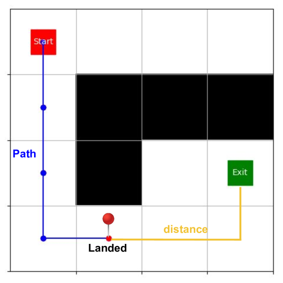
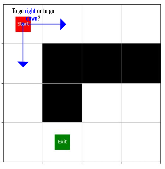
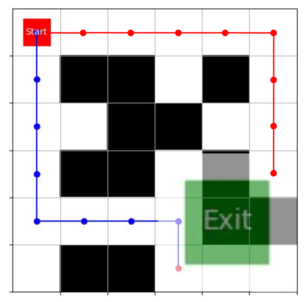
We create a synthetic maze dataset to investigate the causal effect of traversing paths within a maze. The objective is to determine the distance to the exit after following a path. The confounding variable is the start and end positions, the action is the sequence of moves in a path, and the outcome is the distance from the final position to the exit.444 is the shortest distance in the maze while avoiding obstacles, not necessarily the Hamming distance. We compute potential outcomes in two settings: given a path (cf. Figure 2) and given a partial path (cf. Figure 2). The positions of the obstacles are unknown to the model. We run a randomized controlled trial (RCT) in order to determine the ground truth potential outcomes in all experiments.
We train three autoregressive models on three separate datasets and evaluate them in the previously described two settings. The first dataset is the RCT dataset, where we randomly select an exit point and sequence of actions. The remaining two non-RCT datasets are produced using two distinct policy functions respectively. The first, termed offline, only includes paths predicted by a neural network trained to identify optimal maze routes. The second dataset is created as a mixture of the RCT and the offline dataset at different a mixing rate . In total, we construct three datasets with , where and correspond to the RCT and offline dataset respectively.
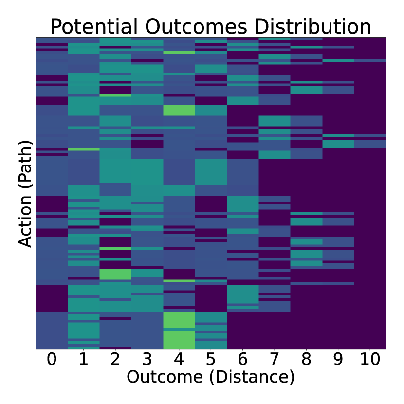
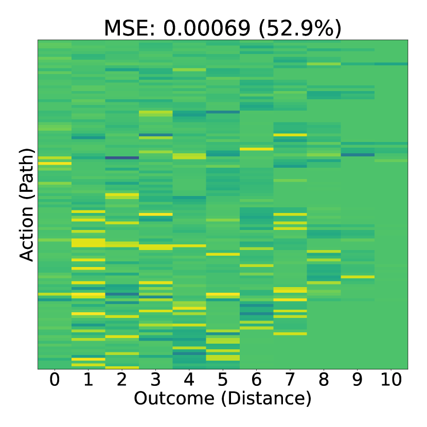
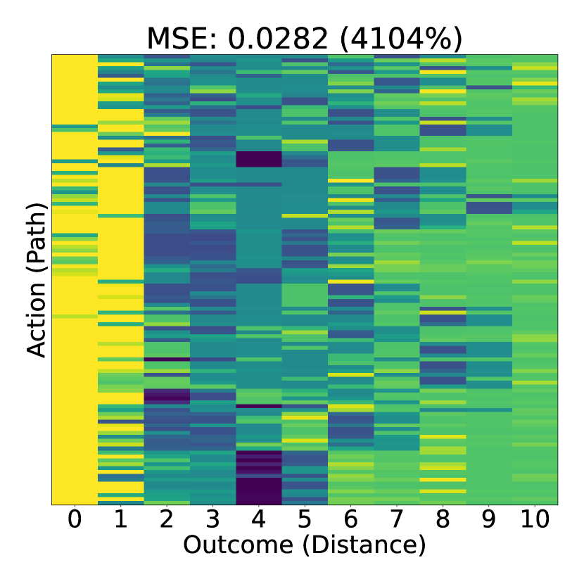
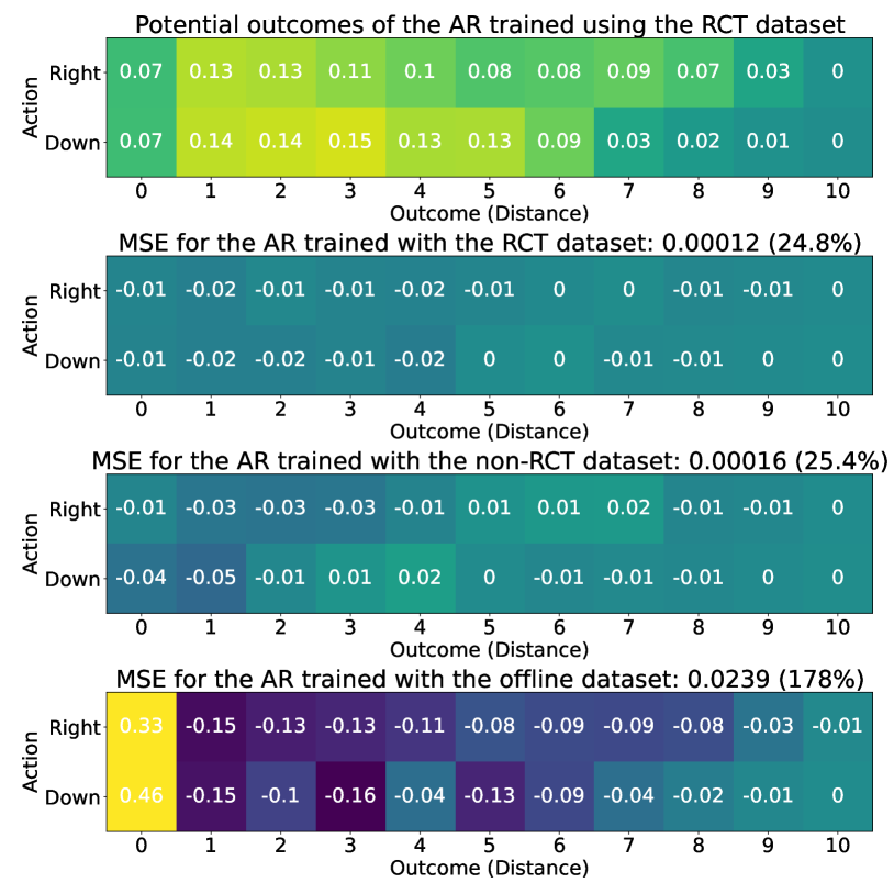
6.1.1 Causal inference using sequential actions
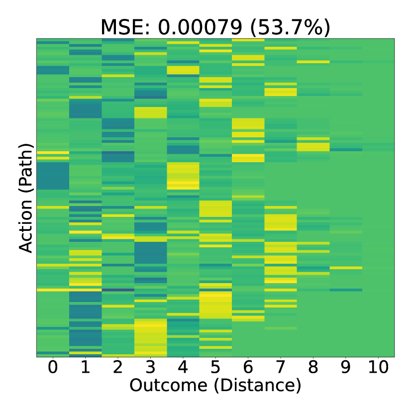
We estimate potential outcomes for possible paths in a maze with a fixed starting point and a maximum length of 6. The maze dimensions are kept small to calculate exact potential outcomes. Figure 3 (a) shows the ground truth potential outcomes for all valid paths. We also compute the mean square error (MSE) and relative error to the empirical RCT estimate. In Figure 3 (b-c), we observe that the estimates closely align with the ground truth for all datasets except . This is because the offline model trained only from optimal moves fails to predict outcomes given a non-optimal path. Hence, autoregressive models generalize even with non-RCT data unless the observed actions are nearly deterministic. Additional experiments on a maze are included in Appendix B.
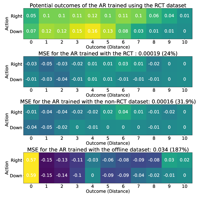
6.1.2 Causal inference using subsequential actions
We consider another question: for a fixed starting state, is it better to go down or right in general (cf. Figure 2)? To answer this, we compute the potential outcome of moving down or right initially. This task is prohibitive for most non-autoregressive CI models as they treat the path as a singular variable. Our model is capable of intervening on any subsequence of actions because the conditional probability of a single action given its parents is computable.
To compute the potential outcome, we marginalize over subsequent actions as shown in Equation 3. Since the paths may be intractable without limiting the maximum length, we cap the longest path to 16 moves as there are a total of 16 positions in the maze. To compare the exact estimates with the Monte Carlo approximations, we report both quantities derived from Equation 3 and 4, and denote them as exact model estimate and approximate model estimate respectively.
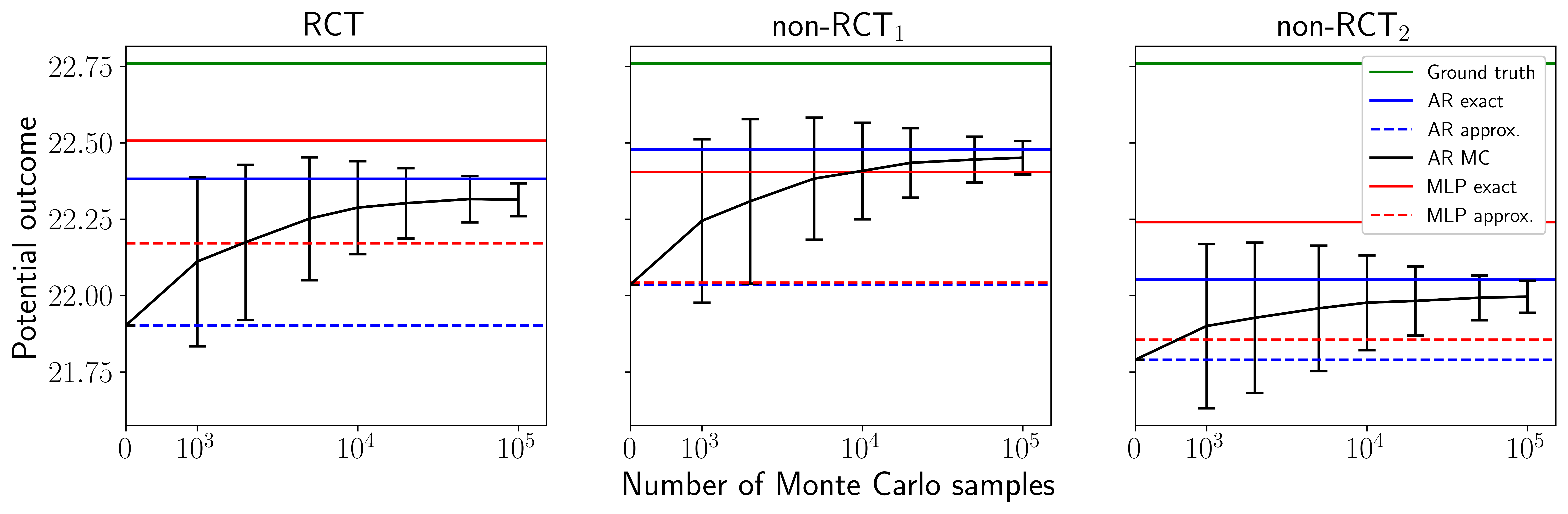
Figure 4 shows the potential outcome estimate of moving right or down initially. The distribution is more concentrated towards smaller distances for moving down and more uniform for moving right. Thus, going down is a better choice for the first move. Furthermore, we observe that and perform similarly, while has a larger MSE because of strictly non-RCT data. More importantly, comparing the exact and approximate model estimates, the Monte Carlo approximation yields similar potential outcomes.
8/8/5r2/2k5/8/4K3/8/8 w - - 0 1 \showboard
6.2 Chess endgame experiments
In this experiment, we analyze a synthetic chess dataset featuring king vs. king-rook endgames with White to move and Black holding the rook. We consider the question: which pieces should Black move on the first two turns to checkmate White the quickest? Using an autoregressive model, we accurately estimate potential outcomes and identify the best action sequence for Black. Furthermore, we use Monte Carlo sampling to obtain better estimates when provided a subset of the data. By answering a query whose solution is not readily apparent, we demonstrate the capability of our proposed causal engine in a more complex and realistic scenario compared to the maze.
Each endgame comprises a two-move chess game, potentially incomplete. The covariate is the initial piece position. The action represents alternating White and Black moves. Since we consider Black’s perspective, we are interested in causal quantities involving and . We assume Black plays optimally after selecting which piece to maneuver, so each action only dictates whether to move the king or the rook, not to which location. The outcome variable is the number of additional moves required to checkmate with optimal play.555In the event of a draw, the outcome is set to 50 due to the 50-move rule. We evaluate the ground-truth outcome using the chess engine Stockfish. An example endgame is shown in Figure 6.
We construct three training datasets: one RCT and two non-RCT sets, denoted non-RCT1 and non-RCT2, with distinct action policies. The RCT dataset uniformly at random selects between moving the king or rook. non-RCT1 and non-RCT2 policy functions are respectively defined as
where is the Hamming distance between the kings. encourages the two kings to be closer while pushes the Black king towards the edge of the board, both of which is required for checkmate. We employ two distinct policies for White between training and testing to evaluate out-of-distribution generalization. White plays uniformly at random over non-optimal moves (unless there are no such legal moves) for the training dataset and only plays optimally in the test set.
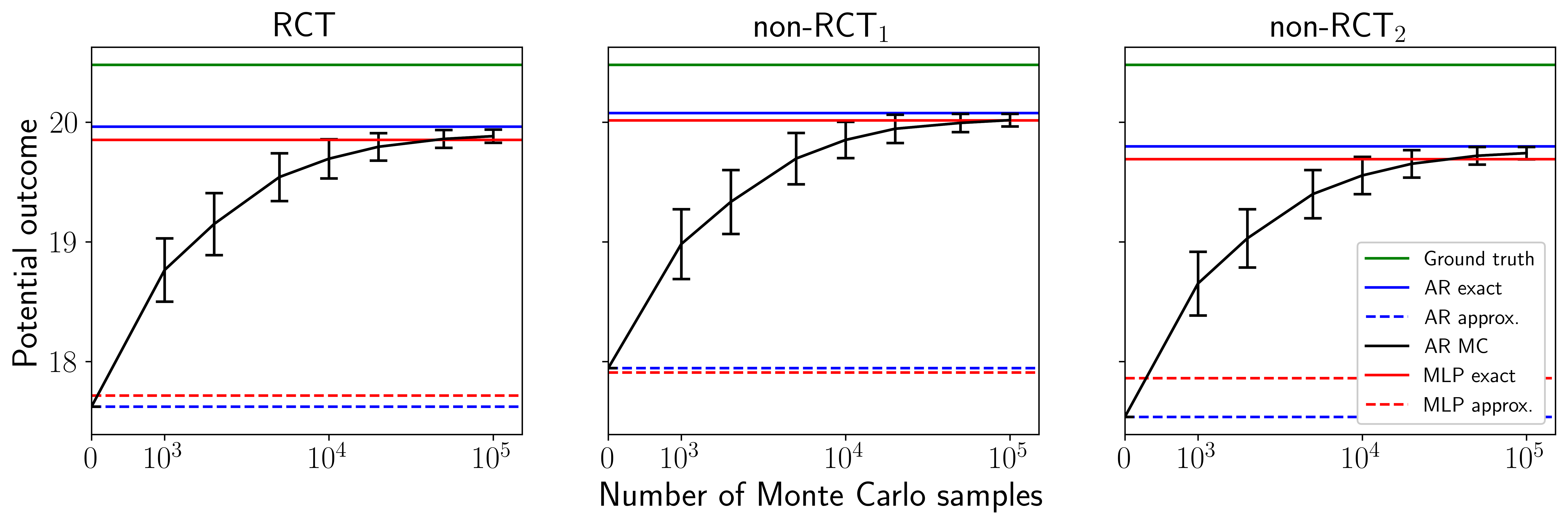
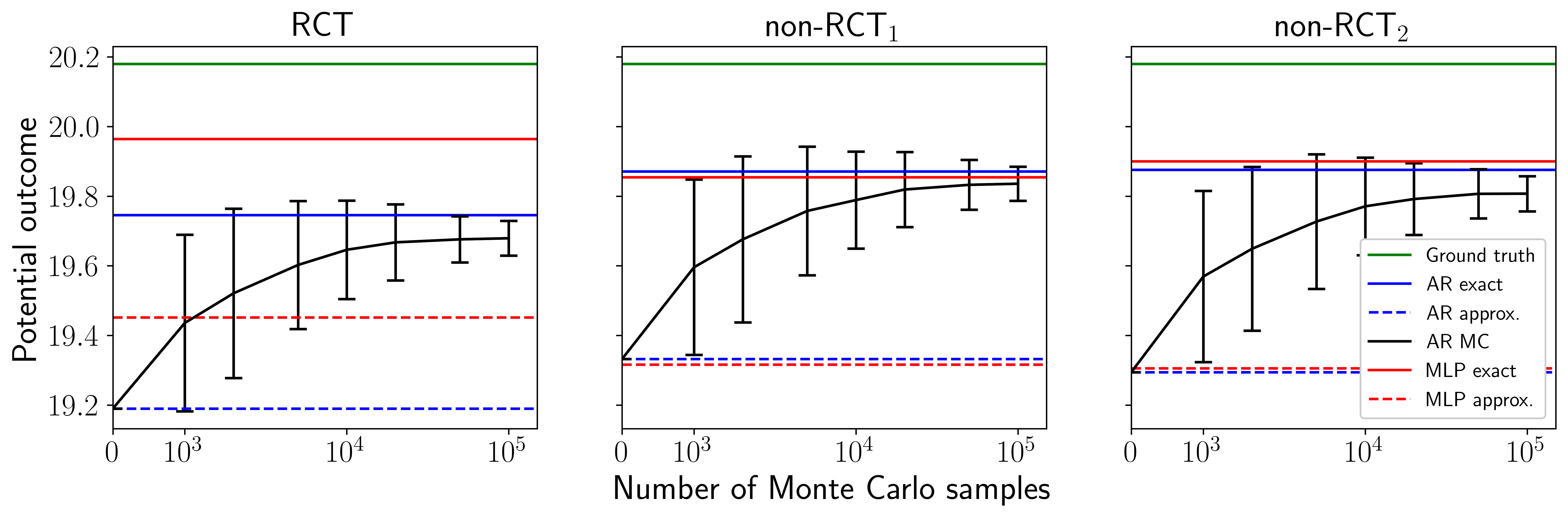
We calculate the ground-truth potential outcomes for all actions and compare them with three different model estimates: the exact model estimate using the entire test dataset, approximate model estimate using a subset of the test data, and Monte Carlo model estimate using the same data subset, but additionally generating samples from the model. The approximate and Monte Carlo estimates correspond to a real-world setting, since obtaining many RCT samples is difficult. Figure 5(b) shows that as we increase the number of samples for Monte Carlo approximation, the potential outcome estimates approach to exact estimate. One reason for the gap between ground truth and AR exact model estimate is due to a distribution shift in between the training and test data. The potential outcomes for the remaining actions are provided in Appendix C. By comparing all potential outcome estimates, we correctly answer our proposed counterfactual query and conclude that moving the rook twice initially is best for Black.
6.3 PeerRead experiments
In this experiment, we use the PeerRead dataset (Kang et al., 2018) to estimate causal effects in a semi-realistic context with high-dimensional confounders. The dataset consists of paper draft submissions to leading computer science conferences such as NeurIPS, ICML, and ICLR, along with acceptance/rejection decisions. We examine the impact of including "theorems" on the likelihood of acceptance. Building on prior work, we focus on computational linguistics, machine learning, and artificial intelligence papers submitted between 2007 and 2017 (Veitch et al., 2020).
The covariate is the paper’s abstract text, the action is a binary variable specifying the presence of the keyword “theorem”, and the outcome is a binary variable indicating acceptance or rejection. To address inaccessible real-world counterfactual outcomes, we follow prior methods by generating synthetic outcomes using the action and the title buzziness (whether the title contains “deep”, “neural”, or “adversarial net”), as shown in Figure 6. For instance, and likely denote a deep learning paper featuring a theorem, whereas and might be a theoretical machine learning paper (or a deep learning paper with a theorem but lacking a buzzy title). (Veitch et al., 2020) has established a correlation between title buzziness and the text.
We compare our proposed approach against Causal-Bert (C-BERT) from (Veitch et al., 2020).666C-BERT learns causally sufficient embeddings, low-dimensional document representations that preserve sufficient information for causal identification and allow for efficient estimation of causal effects. Just like C-BERT, we fine-tune the pre-trained BERT model on our sequencified representations for a fair comparison. We randomly sample subsections of the abstract and fine-tune BERT as if it is a next-token prediction model. Additionally, we use GPT-2 (referred to as GPT) as another pre-trained model (Radford et al., 2019) which has a comparable parameter size to BERT.
Following the original experiment design, we report the Average Treatment Effect on the Treated (ATT) across three confounding levels: low, medium, and high. A positive ATT indicates that including a theorem increases the paper’s chance of acceptance. Table 1 demonstrates that our approach outperforms C-BERT and other benchmarks by significant margins.777We explain the strong performance despite different synthetic and real-world causal graphs in Appendix D. The major difference between C-BERT and our approach is that we do not distinguish between learning representations and the outcome prediction network, and instead train one model to do both In contrast, C-BERT uses multiple objective functions and additional architectural layers.
Our proposed framework is able to exploit the existing knowledge in pre-trained LLMs. Training GPT from scratch fails to identify causal effects, whereas fine-tuning GPT does. By leveraging existing language models, we can estimate causal quantities even under the high-dimensional confounding setting. Consequently, our approach applies to a wider variety of CI tasks and is more capable than non-autoregressive causal models.
| Confounding level | |||
| Low | Medium | High | |
| Ground truth | |||
| Computed biased | (%) | (%) | (%) |
| Reported biased (Veitch et al., 2020) | (%) | (%) | (%) |
| MLP | (%) | (%) | (%) |
| C-BERT | (%) | (%) | (%) |
| C-BERT | (%) | (%) | (%) |
| DARCIE-GPT2 (No pre-train) | () | () | () |
| DARCIE-BERT (Ours) | (%) | (%) | (%) |
| DARCIE-GPT2 (Ours) | (%) | (%) | (%) |
7 Conclusion
In this work, we propose an autoregressive model framework for causal inference capable of handling high-dimensional and combinatorially large variables. In our approach, the key idea is to sequencify data according to the underlying causal DAG and train an autoregressive model to learn conditional distributions. Our experiments show that this method is a unified and robust approach to inferring causal effects.
Despite its effectiveness, our approach has three primary limitations. Firstly, the underlying causal graph must be known. Secondly, all variables in the graph must be observed. Lastly, our approach only supports conditioning or intervening on the prefix of a variable. We leave investigations on overcoming these limitations for future work.
Broader Impact Statement
Our research introduces an deep autoregressive model framework for causal inference, designed to handle high-dimensional data. This method potentially enables scientific discoveries and promotes social fairness by uncovering causal relationships among key variables. However, causal modeling relies on strong assumptions and may not always identify the true causal structure of observational data. Nonetheless, we believe our framework promotes a positive societal impact due to its effectiveness and flexibility over a wider variety of CI applications.
References
- Berenberg et al. (2022) D. Berenberg, J. H. Lee, S. Kelow, J. W. Park, A. Watkins, V. Gligorijević, R. Bonneau, S. Ra, and K. Cho. Multi-segment preserving sampling for deep manifold sampler, 2022.
- Chen et al. (2021) L. Chen, K. Lu, A. Rajeswaran, K. Lee, A. Grover, M. Laskin, P. Abbeel, A. Srinivas, and I. Mordatch. Decision transformer: Reinforcement learning via sequence modeling, 2021.
- Chowdhery et al. (2023) A. Chowdhery, S. Narang, J. Devlin, M. Bosma, G. Mishra, and A. R. et al. Palm: Scaling language modeling with pathways. Journal of Machine Learning Research, 24(240):1–113, 2023. URL http://jmlr.org/papers/v24/22-1144.html.
- Cochran and Rubin (1973) W. G. Cochran and D. B. Rubin. Controlling bias in observational studies: A review. The Indian Journal of Statistics, Series A, 35:417–446, 1973. doi: JSTOR,http://www.jstor.org/stable/25049893.
- Donahue et al. (2020) C. Donahue, M. Lee, and P. Liang. Enabling language models to fill in the blanks, 2020.
- D’Amour et al. (2021) A. D’Amour, P. Ding, A. Feller, L. Lei, and J. Sekhon. Overlap in observational studies with high-dimensional covariates. Journal of Econometrics, 221(2):644–654, 2021.
- Egami et al. (2022) N. Egami, C. J. Fong, J. Grimmer, M. E. Roberts, and B. M. Stewart. How to make causal inferences using texts. Science Advances, 8(42):eabg2652, 2022.
- Garrido et al. (2021) S. Garrido, S. Borysov, J. Rich, and F. Pereira. Estimating causal effects with the neural autoregressive density estimator. Journal of Causal Inference, 9(1):211–228, 2021. doi: doi:10.1515/jci-2020-0007. URL https://doi.org/10.1515/jci-2020-0007.
- Gui and Veitch (2022) L. Gui and V. Veitch. Causal estimation for text data with (apparent) overlap violations. arXiv preprint arXiv:2210.00079, 2022.
- Gupta et al. (2023) K. Gupta, B. Th’erien, A. Ibrahim, M. L. Richter, Q. G. Anthony, E. Belilovsky, I. Rish, and T. Lesort. Continual pre-training of large language models: How to (re)warm your model? ArXiv, abs/2308.04014, 2023. URL https://api.semanticscholar.org/CorpusID:260704601.
- Holland (1986) P. W. Holland. Statistics and causal inference. Journal of the American Statistical Association, 81(396):945–960, 1986. doi: 10.1080/01621459.1986.10478354. URL https://www.tandfonline.com/doi/abs/10.1080/01621459.1986.10478354.
- Im et al. (2021) D. j. I. Im, K. Cho, and N. Razavian. Causal effect variational autoencoder with uniform treatment for overcoming covariate shifts. In arXiv preprint arXiv:2111.08656, 2021.
- Janner et al. (2021) M. Janner, Q. Li, and S. Levine. Offline reinforcement learning as one big sequence modeling problem. In M. Ranzato, A. Beygelzimer, Y. Dauphin, P. Liang, and J. W. Vaughan, editors, Advances in Neural Information Processing Systems, volume 34, pages 1273–1286. Curran Associates, Inc., 2021. URL https://proceedings.neurips.cc/paper_files/paper/2021/file/099fe6b0b444c23836c4a5d07346082b-Paper.pdf.
- Johansson et al. (2018) F. D. Johansson, N. Kallus, U. Shalit, and D. A. Sontag. Learning weighted representations for generalization across designs. arXiv: Machine Learning, 2018.
- Kang et al. (2018) D. Kang, W. Ammar, B. Dalvi, M. van Zuylen, S. Kohlmeier, E. Hovy, and R. Schwartz. A dataset of peer reviews (PeerRead): Collection, insights and NLP applications. In M. Walker, H. Ji, and A. Stent, editors, Proceedings of the 2018 Conference of the North American Chapter of the Association for Computational Linguistics: Human Language Technologies, Volume 1 (Long Papers), pages 1647–1661, New Orleans, Louisiana, June 2018. Association for Computational Linguistics. doi: 10.18653/v1/N18-1149. URL https://aclanthology.org/N18-1149.
- Keith et al. (2020) K. A. Keith, D. Jensen, and B. O’Connor. Text and causal inference: A review of using text to remove confounding from causal estimates, 2020.
- Kocaoglu et al. (2017) M. Kocaoglu, K. Shanmugam, and E. Bareinboim. Experimental design for learning causal graphs with latent variables. In I. Guyon, U. V. Luxburg, S. Bengio, H. Wallach, R. Fergus, S. Vishwanathan, and R. Garnett, editors, Advances in Neural Information Processing Systems, volume 30. Curran Associates, Inc., 2017. URL https://proceedings.neurips.cc/paper/2017/file/291d43c696d8c3704cdbe0a72ade5f6c-Paper.pdf.
- Kumor et al. (2021) D. Kumor, J. Zhang, and E. Bareinboim. Sequential causal imitation learning with unobserved confounders. In M. Ranzato, A. Beygelzimer, Y. Dauphin, P. Liang, and J. W. Vaughan, editors, Advances in Neural Information Processing Systems, volume 34, pages 14669–14680. Curran Associates, Inc., 2021. URL https://proceedings.neurips.cc/paper/2021/file/7b670d553471ad0fd7491c75bad587ff-Paper.pdf.
- Larochelle and Murray (2011) H. Larochelle and I. Murray. The neural autoregressive distribution estimator. In G. Gordon, D. Dunson, and M. Dudík, editors, Proceedings of the Fourteenth International Conference on Artificial Intelligence and Statistics, volume 15 of Proceedings of Machine Learning Research, pages 29–37, Fort Lauderdale, FL, USA, 11–13 Apr 2011. PMLR. URL https://proceedings.mlr.press/v15/larochelle11a.html.
- Liu et al. (2022) T. Liu, Y. E. Jiang, N. Monath, R. Cotterell, and M. Sachan. Autoregressive structured prediction with language models. In Y. Goldberg, Z. Kozareva, and Y. Zhang, editors, Findings of the Association for Computational Linguistics: EMNLP 2022, pages 993–1005, Abu Dhabi, United Arab Emirates, Dec. 2022. Association for Computational Linguistics. doi: 10.18653/v1/2022.findings-emnlp.70. URL https://aclanthology.org/2022.findings-emnlp.70.
- Louizos et al. (2017) C. Louizos, U. Shalit, J. Mooij, D. Sontag, R. Zemel, and M. Welling. Causal effect inference with deep latent-variable models. In arXiv preprint arXiv:1705.08821, 2017.
- Lu et al. (2022) Z. Lu, Y. Cheng, M. Zhong, G. Stoian, Y. Yuan, and G. Wang. Causal Effect Estimation Using Variational Information Bottleneck, pages 288–296. 12 2022. ISBN 978-3-031-20308-4. doi: 10.1007/978-3-031-20309-1-25.
- Monti et al. (2020) R. P. Monti, I. Khemakhem, and A. Hyvarinen. Autoregressive flow-based causal discovery and inference, 2020.
- Mozer et al. (2020) R. Mozer, L. Miratrix, A. R. Kaufman, and L. J. Anastasopoulos. Matching with text data: An experimental evaluation of methods for matching documents and of measuring match quality. Political Analysis, 28(4):445–468, 2020.
- Pearl (2010) J. Pearl. An introduction to causal inference. The international journal of biostatistics, 6:1557–4679, 2010.
- Radford et al. (2019) A. Radford, J. Wu, R. Child, D. Luan, D. Amodei, and I. Sutskever. Language models are unsupervised multitask learners. 2019.
- Roberts et al. (2020) M. E. Roberts, B. M. Stewart, and R. A. Nielsen. Adjusting for confounding with text matching. American Journal of Political Science, 64(4):887–903, 2020.
- Shalit et al. (2017) U. Shalit, F. D. Johansson, and D. Sontag. Estimating individual treatment effect: Generalization bounds and algorithms. ICML’17, page 3076–3085. JMLR.org, 2017.
- Sheng et al. (2023) K. Sheng, Z. Wang, Q. Zhao, X. Jiang, and G. Zhou. A unified framework for synaesthesia analysis. In H. Bouamor, J. Pino, and K. Bali, editors, Findings of the Association for Computational Linguistics: EMNLP 2023, pages 6038–6048, Singapore, Dec. 2023. Association for Computational Linguistics. doi: 10.18653/v1/2023.findings-emnlp.401. URL https://aclanthology.org/2023.findings-emnlp.401.
- Sridhar and Getoor (2019) D. Sridhar and L. Getoor. Estimating causal effects of tone in online debates. In Proceedings of the Twenty-Eighth International Joint Conference on Artificial Intelligence, 2019.
- Tu and Li (2022) H. Tu and Y. Li. An overview on controllable text generation via variational auto-encoders. ArXiv, abs/2211.07954, 2022. URL https://api.semanticscholar.org/CorpusID:253523104.
- Vaswani et al. (2017) A. Vaswani, N. Shazeer, N. Parmar, J. Uszkoreit, L. Jones, A. N. Gomez, Ł. Kaiser, and I. Polosukhin. Attention is all you need. Advances in neural information processing systems, 30, 2017.
- Veitch et al. (2019) V. Veitch, D. Sridhar, and D. M. Blei. Using text embeddings for causal inference. ArXiv, abs/1905.12741, 2019. URL https://api.semanticscholar.org/CorpusID:170079051.
- Veitch et al. (2020) V. Veitch, D. Sridhar, and D. Blei. Adapting text embeddings for causal inference. In J. Peters and D. Sontag, editors, Proceedings of the 36th Conference on Uncertainty in Artificial Intelligence (UAI), volume 124 of Proceedings of Machine Learning Research, pages 919–928. PMLR, 03–06 Aug 2020. URL https://proceedings.mlr.press/v124/veitch20a.html.
- Vinyals et al. (2015) O. Vinyals, L. Kaiser, T. Koo, S. Petrov, I. Sutskever, and G. Hinton. Grammar as a foreign language. In NIPS, 2015. URL http://arxiv.org/abs/1412.7449.
- Wang and Jordan (2021) Y. Wang and M. I. Jordan. Desiderata for representation learning: A causal perspective, 2021.
- Welleck et al. (2019) S. Welleck, K. Brantley, H. D. Iii, and K. Cho. Non-monotonic sequential text generation. In K. Chaudhuri and R. Salakhutdinov, editors, Proceedings of the 36th International Conference on Machine Learning, volume 97 of Proceedings of Machine Learning Research, pages 6716–6726. PMLR, 09–15 Jun 2019. URL https://proceedings.mlr.press/v97/welleck19a.html.
- Xu et al. (2024) M. Xu, W. Yin, D. Cai, R. Yi, D. Xu, Q. Wang, B. Wu, Y. Zhao, C. Yang, S. Wang, et al. A survey of resource-efficient llm and multimodal foundation models. arXiv preprint arXiv:2401.08092, 2024.
- Zhang et al. (2024) P. Zhang, G. Zeng, T. Wang, and W. Lu. Tinyllama: An open-source small language model, 2024.
- Zhong et al. (2022) K. Zhong, F. Xiao, Y. Ren, Y. Liang, W. Yao, X. Yang, and L. Cen. Descn: Deep entire space cross networks for individual treatment effect estimation. Proceedings of the 28th ACM SIGKDD Conference on Knowledge Discovery and Data Mining, 2022.
Appendix A Architecture and training
The maze experiments were conducted on a single NVIDIA GeForce RTX 1080 TI. All models for the chess and PeerRead experiments were trained on a single NVIDIA GeForce RTX 3090 in four and eight hours respectively.
Maze experiments. All three datasets contain 50,000 sequencified data points. We use a vanilla transformer model for the policy and outcome prediction networks consisting of 4 block layers, 32 dimensional 4 multi-heads, and a batch size of 100. We trained 20,000 epochs using Adam for the CI model and 2000 epochs for the policy neural network to avoid overfitting.
Chess endgame experiments. We use a 512-dimensional vanilla transformer, comprising 6 block layers and 8 attention heads. The training task is next-token prediction using the tokenized representation. We train for 200 epochs using the Adam optimizer with a batch size of 4096. The learning rate was selected to be as large as possible without overfitting.
For the training dataset, we sample 500k two-move chess games for each dataset based on Black’s policy function. The test dataset encompasses every game for all 223,660 legal starting positions and all four possible Black actions (king-king, king-rook, rook-king, rook-rook). We sequencify the data by assigning a unique token to every square, legal king and rook move, and outcome.
PeerRead experiments. We fine-tuned our models from the pre-trained BERT and GPT base model checkpoints.888BERT-Base is available at https://huggingface.co/google/bert_uncased_L-12_H-768_A-12 and GPT is available at https://huggingface.co/openai-community/gpt2. We employed a two-phase training process for BERT, analogous to the training of C-BERT. In the initial phase, we focused on training BERT to generate abstracts. The second phase involves training BERT to generate full sequences that include both actions and outcomes. The initial phase is not required for GPT since it was pre-trained on next-token prediction, so training GPT is streamlined into one step. This method ensures a gradual enhancement of the models’ generative abilities, tailored specifically to the PeerRead corpus.
For all training phases, we train for 100 epochs using the Adam optimizer with a batch size of 16. The learning rate and weight decay was chosen at large and small as possible respectively without overfitting. While training the GPT model from scratch, we notice that overfitting occurs regardless of the learning rate or weight decay.
We elaborate on the synthetic outcome generation process (cf. Figure 6). Following [Veitch et al., 2020], the synthetic outcome is expressed as
where is a sigmoid function, is a proportional to in each paper, and controls the level of confounding. Low, medium, and high confounding levels in this work correspond to , , and respectively. Higher indicates the outcome is more correlated to the title buzziness instead of the action , so the ground-truth ATT is smaller. Note that the PeerRead dataset is imbalanced with more non-buzzy papers than buzzy ones.
Appendix B Maze extra experiments
B.1 Comparing two paths on 6x6 Maze
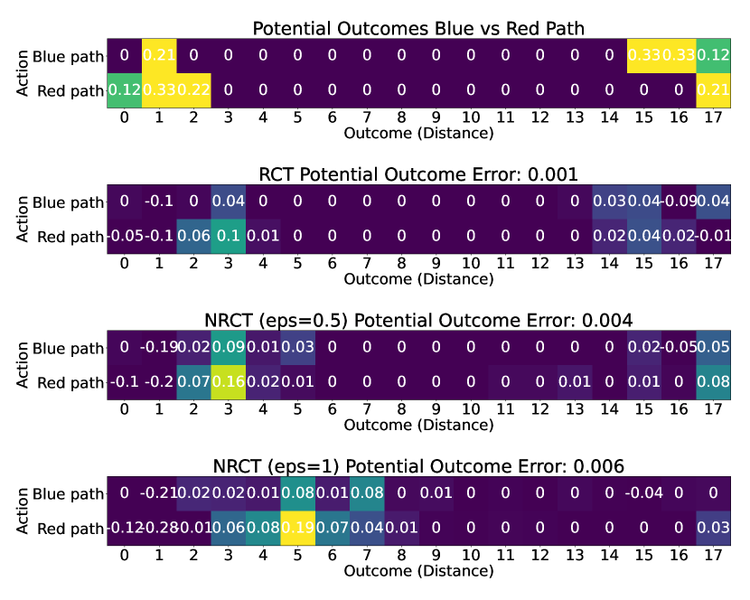
We consider a larger maze featuring two distinct paths as illustrated in Figure 9. For this setup, we compute potential outcomes given a set of valid exit points instead of a single exit point. During the training phase, the exit location is randomly chosen within the maze; however, during testing, it is restricted to the bottom-right quadrant. Taking the red path is far away from all but one exit, whereas taking the blue path is close to all but one exit. The first heat map in Figure 9 depicts potential outcome estimates for both paths, with outcomes ranging from 0-2 and 16 for the blue path and 0-15 to 17 for the red path, aligning with the intuition from Figure 9. Subsequent heat maps display the potential outcome MSE.
Appendix C Chess endgames extra experiments
C.1 Potential outcome estimates
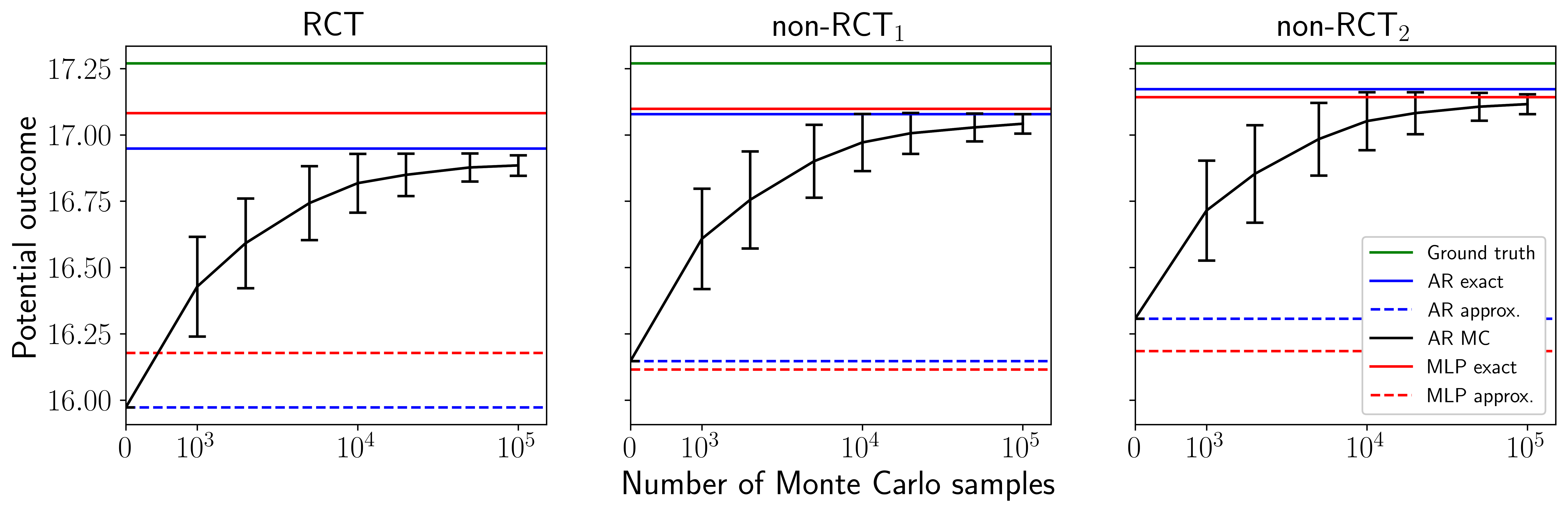
We present the potential outcome graphs for the remaining three possible actions: king-king, king-rook, and rook-rook in Figure 10. The model behavior on these actions closely align with the observations for rook-king in Figure 5(b), indicating that Monte Carlo sampling is effective across various interventions. For all actions, using Monte Carlo sampling achieves better potential outcome estimates when only a subset of the data is available.
We compare the potential outcome values for all actions in Table 2. We include the exact model estimates and approximate model estimates. Our autoregressive model performs similarly to the baseline in both these metrics. Hence, our proposed approach adeptly models the outcome, and simultaneously is capable of using Monte Carlo sampling to improve predictions when data is limited. Furthermore, the predictions from all models align with the ground-truth answer to our counterfactual query: on average, moving the rook twice initially leads to checkmate the fastest.
| Potential outcome (Error %) | |||||
|---|---|---|---|---|---|
| king-king | king-rook | rook-king | rook-rook | ||
| Ground truth | |||||
| RCT | () | () | () | () | |
| MLP exact | non-RCT1 | () | () | () | () |
| non-RCT2 | () | () | () | () | |
| RCT | () | () | () | () | |
| MLP approx. | non-RCT1 | () | () | () | () |
| non-RCT2 | () | () | () | () | |
| RCT | () | () | () | () | |
| AR exact | non-RCT1 | () | () | () | () |
| non-RCT2 | () | () | () | () | |
| RCT | () | () | () | () | |
| AR approx. | non-RCT1 | () | () | () | () |
| non-RCT2 | () | () | () | () | |
Appendix D PeerRead extra experiments
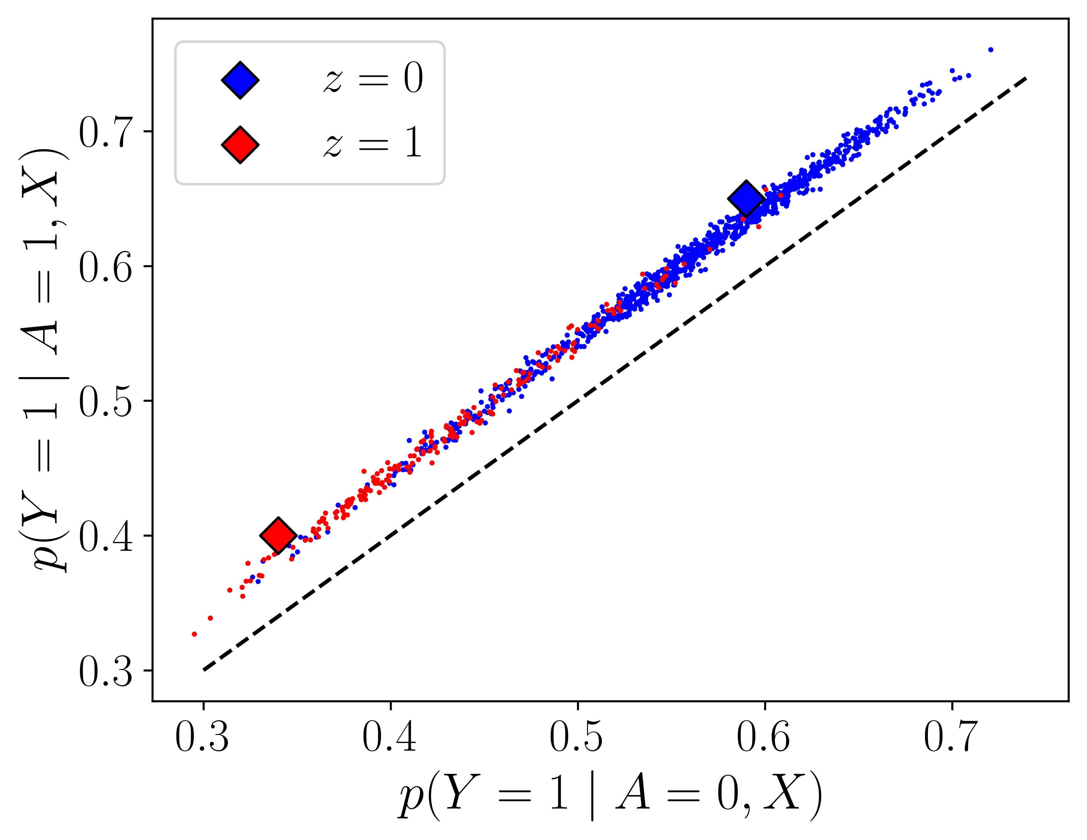
To illustrate the positive predicted ATT on the PeerRead dataset, we compare against for all data points using GPT in Figure 12. Our model consistently favours papers containing theorems, regardless of title buzziness.
Additionally, we investigate why our model has strong performance when the outcome is generated from and (cf. Figure 6), while the input is and (cf. Figure 6). We quantify the correlation between the title buzziness and the abstract by training a logistic regression to predict from . For each of our models, we take the final hidden layer output as the vectorized representation of the abstract. We also train a baseline logistic regression model using the bag-of-words (BoW) representation for . Table 12 demonstrates that and are highly correlated, explaining the high accuracy of potential outcome estimations.
| Accuracy | Balanced accuracy | |
|---|---|---|
| BoW | ||
| BERT | ||
| GPT2 |