Multi-platoon car-following models with flexible platoon sizes and communication levels

Abstract

In this paper, we extend a single platoon car-following (CF) model to some multi-platoon CF models for connected and autonomous vehicles (CAVs) with flexible platoon size and communication level. Specifically, we consider forward and backward communication methods between platoons with delays. Some general results of linear stability are mathematically proven, and numerical simulations are performed to illustrate the effects of platoon sizes and communication levels, as well as to demonstrate the potential for stabilizing human-driven vehicles (HDVs) in mixed traffic conditions. The simulation results are consistent with theoretical analysis, and demonstrate that in the ring road scenario, CAV platoons can stabilize certain percentage of HDVs. This paper can provide suggestions for the design of communication system of autonomous vehicles (AVs), and management of mixed traffic flow of CAVs and HDVs.

I Introduction

Platooning is a coordinated driving strategy that keeps a short distance between vehicles, which can enhance capacity, safety and flow rate of traffic networks. It can be conceptualized as a longitudinal traffic control system [1]. With the recent advancements in connected and autonomous vehicles (CAVs) and associated communication technologies, the era of mixed autonomy, where CAV platoons and human-driven vehicles (HDVs) share the road, is fast approaching. To model such mixed-autonomy environments, one common choice is microscopic traffic flow models, e.g. car-following (CF) models, which provide a useful framework for researchers to study the interactions and dynamics between CAVs and HDVs under varying traffic conditions.

Car-following (CF) models have been fundamental to traffic flow theory since Pipes introduced the first operational model in 1953 [2]. Following this, several CF models were developed to incorporate more realistic dynamics. Notably, the Optimal Velocity Model (OVM) proposed by Bando et al. [3, 4] replaced the leading vehicle’s velocity in Pipes’ model with an optimal velocity function. The Intelligent Driver Model (IDM), introduced by Treiber et al. [5], further improved upon these models by considering the velocity difference between the lead and following vehicles. These early-stage CF models are widely used in traffic simulations and control design, since they are capable of describing typical traffic phenomena with relatively simple forms. Several extensions have been proposed for these models, e.g. [6], [7], and [8]. However, these models limits the interaction between a pair of vehicles in a leader-follower configuration. Extensions are necessary for these models to describe more complicated traffic scenarios involving CAVs.

The next stage of CF models includes multi-vehicle interaction, moving beyond the classic models considering only the immediate leader, thus modeling traffic flow more realistically.CF patterns such as multi-following [9] and backward-following [10], both based on OVM, have been increasingly explored and have inspired subsequent research on mixed traffic flow [11], [12], where CAVs are designed to better stabilize traffic. In fully autonomous traffic scenarios, various platooning designs can be integrated to enhance both efficiency and safety [13], [14], [15], [16, 17], [18]. Further improvements to CF models include the addition of delay factors [19], [20], as well as the integration of control mechanisms such as safety-prioritized control [21, 22] and feedback control [23]. These extended CF models, coupled with advanced control strategies, reflect the growing trend on improving traffic stability, efficiency, and safety. By accounting for multi-vehicle interactions and integrating autonomous systems, these models contribute significantly to enhancing traffic performance, particularly in mixed autonomy scenarios.

Control strategies for groups of CAVs, particularly ACC and Cooperative Adaptive Cruise Control (CACC), have been extensively studied to improve vehicle platooning efficiency and safety [24, 25]. ACC primarily focuses on maintaining safe distances between vehicles by adjusting speed based on sensor data, achieving better results than typical human drivers. However, it operates in a decentralized manner without relying on vehicle-to-vehicle (V2V) communication. On the other hand, CACC utilizes V2V communication to enable more precise control and coordination among CAV platoons [26, 27, 28]. Additionally, the quality of communications plays a crucial role in the stability of CAV platoons, as shown in studies on robust communication and stability analysis [29, 30, 31]. These studies highlight the advantages of CACC over ACC, particularly regarding communication and coordination within platoons.

Beyond ACC and CACC, advanced control strategies such as Model Predictive Control (MPC), reinforcement learning (RL), and stochastic optimization have been explored to further enhance the performance of CAV platoons in complex traffic scenarios. MPC has been widely used due to its ability to predict future states and optimize control actions over a finite horizon [32, 33, 34]. Meanwhile, RL has increasingly gained attention for its ability to adaptively learn control policies from data, allowing for more flexible and autonomous decision-making in dynamic environments [35]. Stochastic optimization approaches have also been applied to account for uncertainties in traffic behavior and communication, as seen in the work of Li [36, 37].

Field experiments can further demonstrate the effectiveness of CAVs and platooning in increasing traffic stability and reducing fuel consumption. Various configurations, such as a single CAV leading multiple HDVs on a ring road [38], three trucks on a test track [39], and 100 CAVs on a freeway network [40], have been explored by researchers to highlight the benefits of integrating CAVs and platooning into traffic systems. The data generated from such field experiments can also provide valuable insights for theoretical research, as demonstrated in studies like [41] and [42]. These studies underscore the potential of advanced control techniques to further enhance the performance and adaptability of CAVs and platooning, especially in mixed autonomy settings.

Despite the growing trend of investigating the stability of longitudinal interactions among multiple CAV platoons, few studies have explored their implications using ODE-based CF models or in mixed traffic scenarios involving HDVs. To address this research gap, this paper propose a foundational framework for multiple platoons of CAVs that is adaptable to various CF models and control designs. We extend a recently proposed single-platoon CF model [18] to a multi-platoon model that accommodates different control strategies and communication capabilities between platoons. Particularly, when the platoon size is set uniformly to one, the model degenerates to a classic CF model for HDVs, or AVs equipped with backward detection. Theoretically, we demonstrate that the stability of the multi-platoon models depends on the platoon size and communication level: larger platoon sizes and enhanced communication contribute to increased stability, while minimal delays between platoons have a negligible effect on stability. Numerical simulations on a ring road, involving different vehicle arrangements and mixed traffic scenarios with various sizes of CAV platoons and HDVs in different ratios and orders, support our theoretical findings. The simulation results also demonstrate that HDVs benefit from following CAV platoons, even when the CAV platoons are not specially designed to control the HDVs.

The remaining part of this paper is organized as follows. In II, we introduce the CF models for single and multiple platoons of CAVs. In III, stability criteria of the proposed models are presented and proved. In section IV, we perform numerical simulations for the proposed models with various traffic assignments on a ring road. The impact of delay and connectivity are analysed. Lastly in section V, conclusion and possible extensions are given.

II Models for CAV platoons

II-A General assumptions

We assume that there are $m$ CAV platoons on a single lane road with no overtaking allowed, where $m\geq 1$. The $m$-th platoon is the leading platoon, and $N_{i}$ denotes the size of the $i$-th platoon. Within the $i$-th platoon the $N_{i}$-th car is the leading vehicle. Moreover, if the single lane road is a ring road, the $m$-th platoon is following the $1$st platoon.

We select the commonly used Optimal Velocity Model (OVM) [3] as the base CF model for human driven vehicles (HDVs). The OVM is expressed as

$$\ddot{x}_{i}(t)=a\left[V(x_{i+1}(t)-x_{i}(t))-\dot{x}_{i}(t)\right],$$ (1)

where $x_{i}(t)$, $i=1,2,\dots N$ is the position of $i$-th vehicle at time $t$. $x_{i+1}(t)-x_{i}(t)\triangleq h_{i}(t)$ represents the headway between the $i$-th and $i+1$-th vehicle. $\dot{x}_{i}(t)$, $\ddot{x}_{i}(t)$ denotes the velocity and acceleration of the $i$-th vehicle at time $t$, respectively. $V(h)$ is the optimal velocity function of headway (head to head distance) $h$, and $a$ is a sensitivity constant. An example of optimal velocity function is as follows:

$$V(h)=\begin{cases}v_{f},&\text{if }h\geq h_{f};\\ \frac{v_{f}}{2}\left(1-\cos\left(\pi\frac{h-h_{s}}{h_{f}-h_{s}}\right)\right),&\text{if }h_{s}\leq h\leq h_{f};\\ 0,&\text{if }h\leq h_{s},\end{cases}$$ (2)

where $h_{s}$ is the standstill headway, $h_{f}$ is the free flow headway, $v_{f}$ is the free flow speed and $l$ is the length of each vehicle. This is equivalent to the function in [12]. Figure 1 is an example plot of (2) and the corresponding fundamental diagram (density-flow diagram) as in [18].

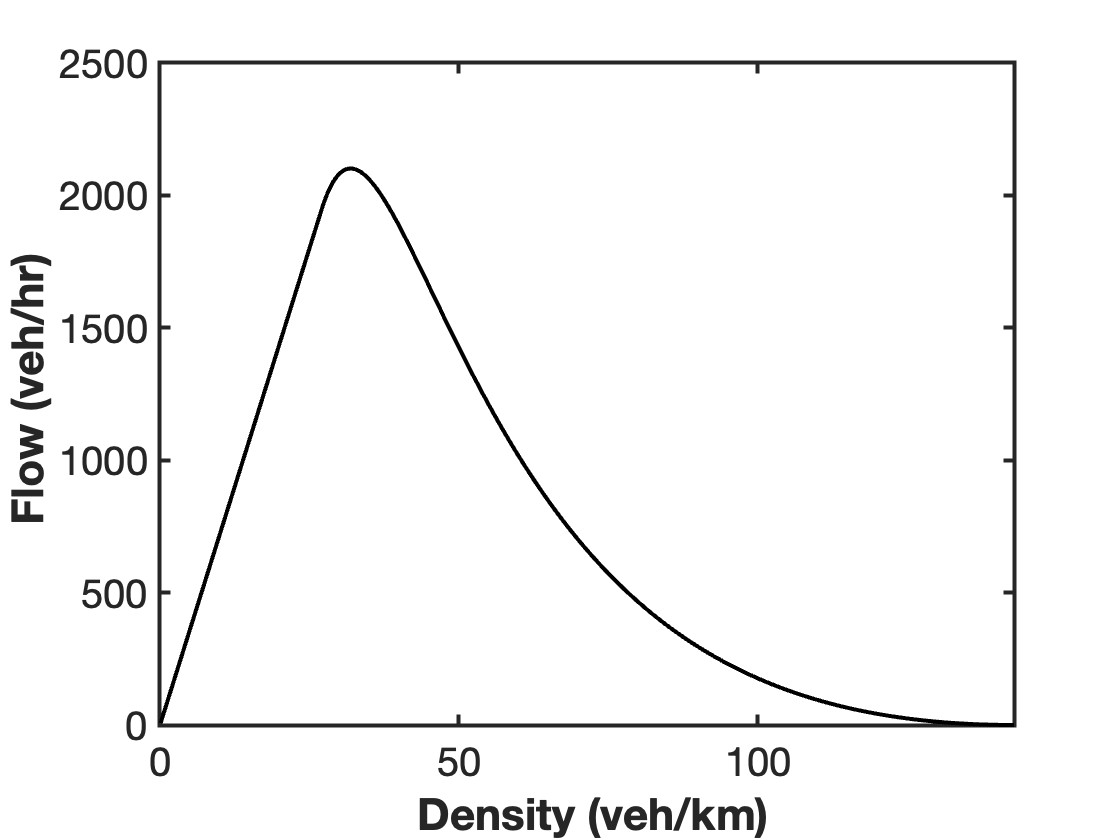
(a) Optimal velocity function

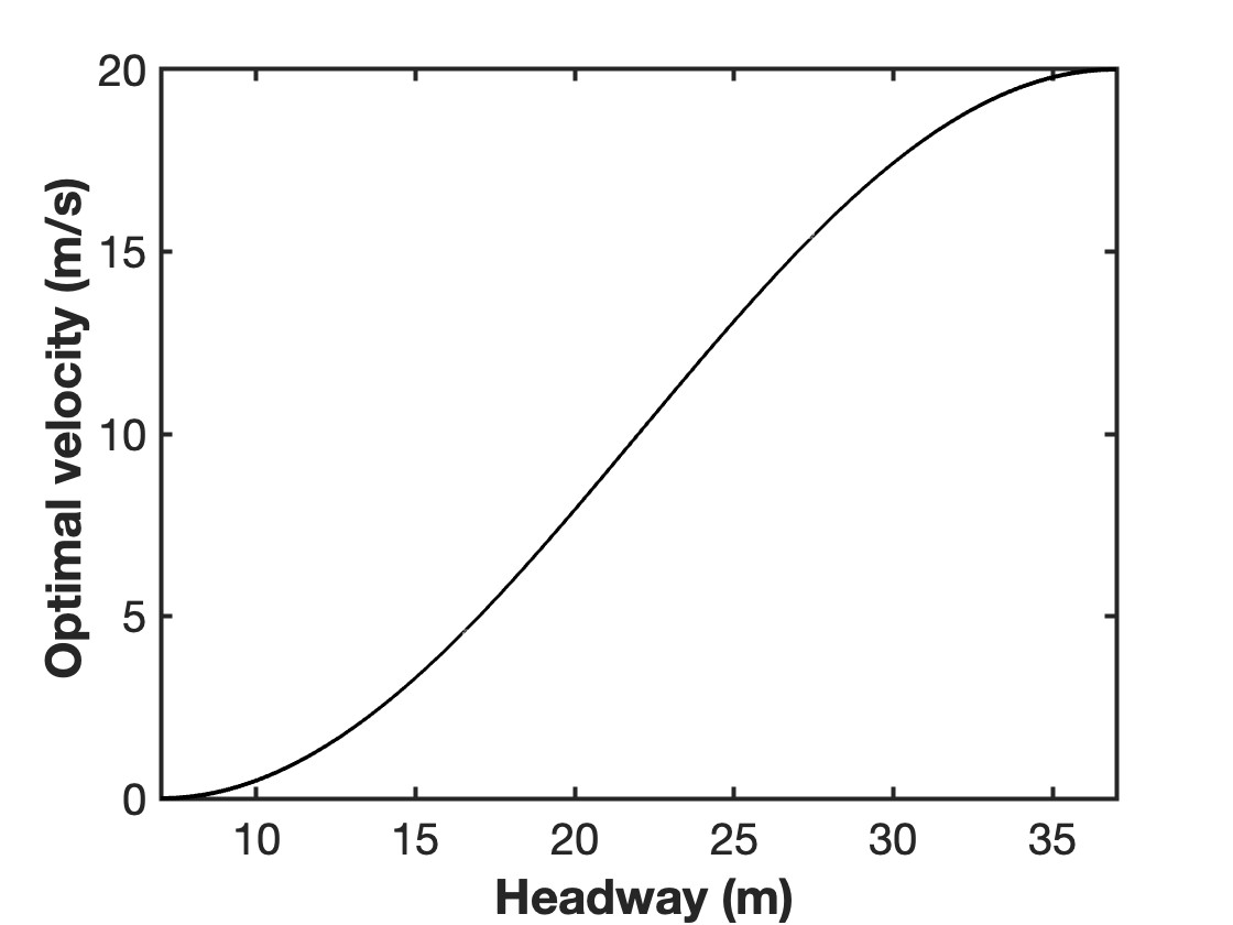
(b) Fundamental diagram

Figure 1: Plot of an optimal velocity function and the corresponding fundamental diagram.

II-B Single platoon: base model

Before investigating multi-platoon models, it is essential to develop a robust single-platoon CF model. In [18], it is shown that if a platoon is sufficiently close to its equilibrium state, the platoon controlled OVM (P-OVM) is always stable under small initial disturbances and periodic disturbances. The proposed model is of the form

$$\ddot{x}_{i}(t)=a\left[V(\frac{x_{N}(t)-x_{i}(t)}{N-i})-\dot{x}_{i}(t)\right],\;i=1,2,\dots,N$$ (3)

where $N$ represents the platoon size, and $x_{N}$ is the position of the controlled leading vehicle. Figure 2 is a visual interpretation of this model.

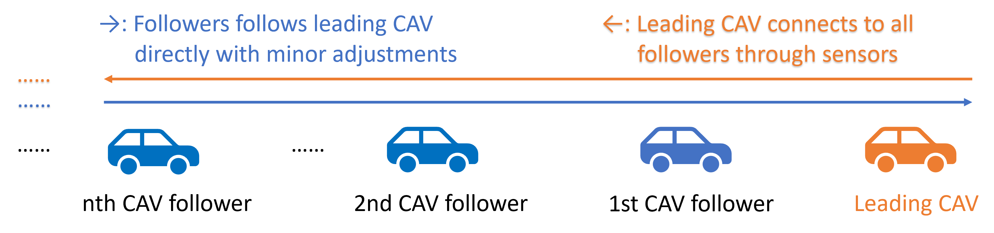
Figure 2: CF pattern of a single platoon

However, the reliability of (3) assumes that platoon followers can precisely acquire information from the leading vehicle with no delay, which is unrealistic for a large number of CAVs. Therefore, a multi-platoon system (where one platoon follows annother) serves as a viable formation strategy for managing long strings of vehicles, helping to mitigate the effects of communication delays and instabilities in centralized controls. In the following subsections, we provide some examples of multi-platoon models where we assume that each platoon is governed by (3) and the speed of platoon leaders are controlled as inputs. We will neglect the effects of communication delays and minor adjustments within each platoon.

II-C Multi-platoon: no inter-connection

If there is no communication between platoons, we assume that the leading vehicle of each platoon only follows the last vehicle of the platoon ahead, as shown in Figure 3.

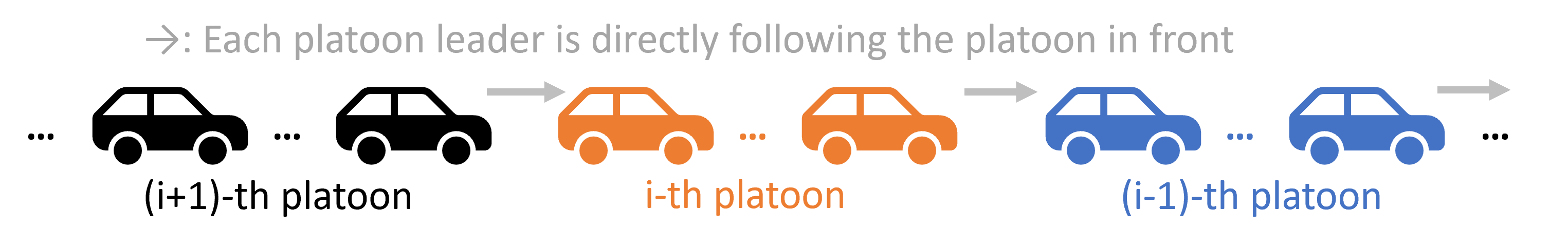
Figure 3: CF pattern of multiple platoons with no inter-platoon communication.

If no additional control is applied, the platoon leaders are directly following the vehicle ahead according to the OVM:

$$\ddot{x}_{i,N_{i}}=a(V(x_{i+1,1}-x_{i,N_{i}})-\dot{x}_{i,N_{i}}),$$ (4)

where $1\leq i\leq m-1$. For the followers within each platoon, the centralized platoon controller (3) is applied:

$$\ddot{x}_{i,j}=a\left[V\left(\frac{x_{i,N_{i}}-x_{i,j}}{N_{i}-j}\right)-\dot{x}_{i,j+1}\right],$$ (5)

where $1\leq i\leq m$ and $1\leq j\leq N_{i}-1$. In particular, if we have platoon size $N_{m}=1\text{ or }2$ for all $m$, the proposed model reduces to the OVM for HDVs.

II-D Multi-platoon: two-way inter-connection

In this subsection we suppose each platoon can communicate with platoons ahead and behind, with some delays (i.e. the platoons are two-way connected), as shown in Figure 4.

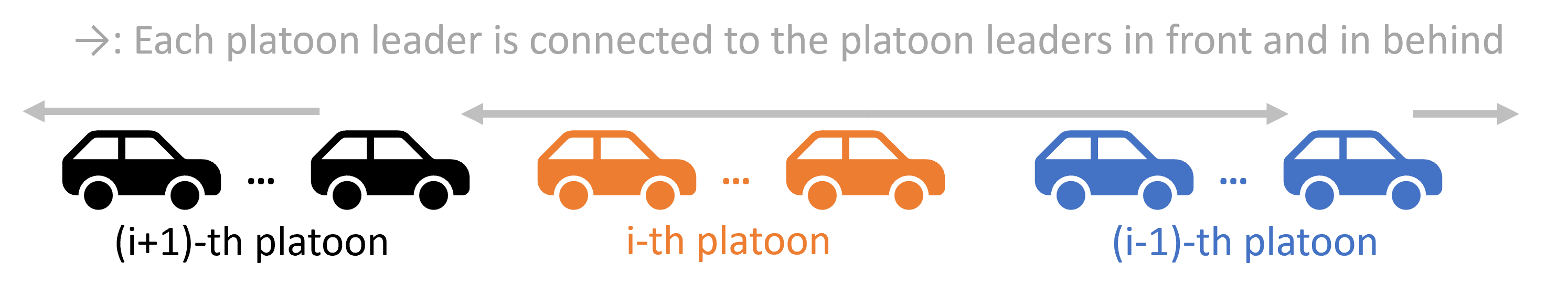
Figure 4: CF pattern of multiple platoons with forward and backward inter-platoon communication.

In this case, we can model the platoon leaders to follow both the platoon in front and the one behind, similar to the model for autonomous vehicles proposed in [11]:

$$\ddot{x}_{i,1}=a \left[(1+p)V\left(\frac{\Delta_{i}(t-t_{d})}{N_{i}}\right)\right.$$ (6)

$$\left.-pV\left(\frac{\Delta_{i-1}(t-t_{d})}{N_{i-1}}\right)-\dot{x}_{i,1}\right],$$

where $\Delta_{i}(t)=x_{i+1,1}(t)-x_{i,1}(t)$ is the headway between the $i$-th and $i+1$-th platoon leader, $p$ is the smoothing factor for the platoon in the back, and $t_{d}$ is the constant communication delay between platoons. For the followers we apply the same equation (5) as in the previous model. In particular, if the platoon size $N_{m}=1$ and $t_{d}=0$ for all $m$, (6) becomes equivalent to the modified OVM with autonomous vehicles in [11].

Remark 1.

The proposed frame work can be applied to any general second order CF models and combined with control strategies such as delayed feedback control, CACC, MPC, etc. However, the main focus of this paper is to present a basic framework for multi-platoon CAVs, so we have kept the models as simple as possible with minimal parameters.

III Stability analysis

In this section, we analyse the stability of the models in section II through linear stability analysis. The steady-state (equilibrium) solution of all the aforementioned models on a ring road of length $L$ with $N_{tot}=\sum_{i=1}^{m}N_{i}$ vehicles is

$$e_{i,j}(t)=h(N_{1}+\dots+N_{i-1}+j)+V(h)t,$$ (7)

where $h=L/N_{tot}$ is the equilibrium headway. To analyse the effect of platoon sizes, for the stability analysis we assume that for the multi-platoon models all the platoons are of a uniform size, denoted as $N$. Then for the no-connection model proposed in Subsection II-C, the following stability criterion holds:

Theorem III.1.

The no-connection multi-platoon model (4, 5) with identical platoon size $N$ is stable if

$$a>\frac{2NV^{\prime}(h)}{(N-1)^{2}+1}.$$ (8)

Proof.

Assume that for each vehicle there is a small deviation from the equilibrium solution:

$$x_{i,j}(t)=e_{i,j}(t)+y_{i,j}(t),\;|y_{i,j}|\ll 1.$$ (9)

Since the platoon leader is just following the last vehicle of the platoon in front, for the first and last vehicle of each platoon they formulate an sub-system of ODEs of $2m$ equations. And we can linearize the sub-system by doing Taylor expansion of $y_{i,j}$ and neglect higher order terms to get

$$\ddot{y}_{i,1}(t)=a\left[(V^{\prime}(h)\frac{y_{i,N}(t)-y_{i,1}(t)}{N-1}-\dot{y}_{i,1}(t)\right]$$ (10)

for platoon leaders, and

$$\ddot{y}_{i,N}(t)=a\left[(V^{\prime}(h)(y_{i+1,1}(t)-y_{i,N}(t))-\dot{y}_{i,N}(t)\right]$$ (11)

for the platoon tails, where $i$ is referring to all the integers that satisfies $1\leq i\leq m$ throughout the proof. The $(m+1)$-th platoon is the same as the $1$st platoon. Then if $\lambda$ is an eigenvalue of the linear ODE system, and $\xi_{i,j}$ are the corresponding coefficients of $y_{i,j}$, simplified from (10, 11) we have

$$\lambda^{2}+a\lambda-aV^{\prime}(h)(\frac{\xi_{i+1,1}}{\xi_{i,N}}-1)=0,$$ (12)

and

$$\lambda^{2}+a\lambda-aV^{\prime}(h)(\frac{\xi_{i,N}}{(N-1)\xi_{i,1}}-\frac{1}{N-1})=0.$$ (13)

Then with the same $\lambda$, the constant parts of (12) and (13) are identical, and we can denote it by $r$. Then the real parts of $\lambda$ can be rewritten as

$$\text{Re}(\lambda)=\frac{1}{2\left(-a+\sqrt{(\frac{d+\sqrt{d^{2}+e^{2}}}{2})}\right)},$$ (14)

where $d=a^{2}+4\text{Re}(r)$ and $e=4\text{Im}(r)$. The sub-system (10, 11) is stable if $\text{Re}(\lambda)<0$, which can be simplified to

$$a>\left|\frac{\text{Im}^{2}(r)}{\text{Re}(r)}V^{\prime}(h)\right|.$$ (15)

Now it remains to show (8) implies (15). Note that

$$\prod_{i=1}^{m}\frac{\xi_{i+1,1}}{\xi_{i,N}}\frac{\xi_{i,N}}{\xi_{i,1}}=1$$ (16)

holds since $m+1=1$ on the ring road, combining with (12, 13) we have $r$ satisfies

$$((N-1)r+1)^{m}(r+1)^{m}=1.$$ (17)

Then we can solve for $r$ to get

$$r=\frac{-N\pm\sqrt{N^{2}-4(N-1)(1-\exp(\frac{2\pi ki}{m}))}}{2(N-1)},$$ (18)

where $k=1,2,\dots,m$. Let $\theta=\frac{2\pi k}{m}$ and $l=1/(N-1)$, then

$$-\frac{\text{Im}^{2}(r)}{\text{Re}(r)}=\frac{\sqrt{d_{2}^{2}+e_{2}^{2}}-d_{2}}{l+1\pm\sqrt{\frac{\sqrt{d_{2}^{2}+e_{2}^{2}}+d_{2}}{2}}},$$ (19)

where $d_{2}=(l+1)^{2}-4l(1-\cos\theta)$ and $e_{2}=4l\sin\theta$. Therefore (19) can be considered as a function of $\theta$, and for $l<1$ this is a decreasing function for $\theta>0$. Then we can obtain

$$\left|\frac{\text{Im}^{2}(r)}{\text{Re}(r)}\right|<\lim_{\theta\to 0^{+}}\left(-\frac{\text{Im}^{2}(r)}{\text{Re}(r)}\right)=\frac{2N}{(N-1)^{2}+1}.$$ (20)

Combined (20) with (15), the sub-system (10, 11) is stable if the stability criterion (8) holds. For the remaining vehicles inside each platoon, the solution is only determined by the leading vehicle of the platoon. And by linearization of (5) we can rewrite $y_{i,j}$ as

$$y_{i,j}=\left(N-j+\frac{j-1}{N-1}\right)y_{i,N},$$ (21)

which is a linear function of $y_{i,N}$. This means the stability of the multi-platoon system is the same as the sub-system (10, 11). Therefore stability criterion (8) holds. ∎

Figure 5 is the plot of stability regions with different platoon size of the no-connection model.

Remark 2.

For all the stability plots, each neutral stability line separates the graph into two regions: the region above the line is unstable and the region below the line is stable.

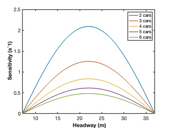
Figure 5: Neutral stability lines of the multi-platoon model with no connection of platoon size $N=2,3,4,5,6$.

Using similar approaches, for the two-way connected model proposed in Subsection II-D, the following stability criterion applies:

Theorem III.2.

The two-way connected multi-platoon model (6, 5) with identical platoon size $N$ is stable if

$$a>\frac{2V^{\prime}(h)}{(1+2p)(N-2t_{d}V^{\prime}(h))}.$$ (22)

Proof.

For the connected model (6, 5) we follow the assumptions of previous works, e.g. [43, 44] such that higher orders of the constant delay $t_{d}$ are neglected. And after linearization, for the connected multi-platoon system in Subsection II-D, The $m$ platoon leaders forms a system of $m$ linear ODEs:

$$\ddot{y}_{i,N}(t)=a \left[V^{\prime}(h)(1+p)\frac{\Delta_{i,N}(t-t_{d})}{N}\right.$$ (23)

$$\left.-V^{\prime}(h)p\frac{\Delta_{i-1,N}(t-t_{d})}{N}-\dot{y}_{i,N}(t)\right].$$

Then if $\lambda$ is an eigenvalue of the system, by reserving first order of $t_{d}$ via Taylor expansion, we have

$$\lambda^{2}+a(1+2p)\lambda-(1-\lambda t_{d})\frac{aV^{\prime}(h)}{N}(1-e^{i\theta})=0,$$ (24)

where $\theta$ is the same as in the proof of Theorem 8. Then by simplifying the condition $\text{Re}(\lambda)<0$, the stability criterion is equivalent to

$$4k(1-\cos\theta)+8at_{d}k^{2}(1-\cos\theta)^{2}>k^{2}\sin^{2}\theta,$$ (25)

where $k=a/(N\cdot V^{\prime}(h))$. Then let $\theta\to 0$ we can get the stability criterion given in Equation 22. ∎

Figure 6 is the plot of the front connected model’s stability regions ($p=0,t_{d}=0$).

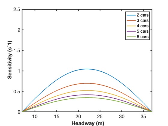
Figure 6: Neutral stability lines of the multi-platoon model with front connection of platoon size $N=2,3,4,5,6$ and zero-delay.

We observe that the connected model exhibits larger stability regions than the non-connected model. However, the difference diminishes as platoon size increases. Figure 7 is the plot of the two-way connected model’s stability regions with different delays of backward sensitivity $p=0.3$ and platoon size $N=4$.

Figure 7: Neutral stability lines of the multi-platoon model with two-way connection of platoon size $N=4$ and delay $t_{d}=0,0.4,0.8,1.2,1.6$s.

From this figure, we can observe that the effect of delay become larger as it get close to $1.6$s. Additionally, if the delay reach $2$s then the model becomes consistently unstable for headways between $20$ and $25$ meters.

Remark 3.

For the effect of backward sensitivity $p$ we refer to [10, 11].

IV Numerical simulations

IV-A General information

We use MATLAB 2024a for both simulation and plots. All the simulations are performed on a single-lane ring road. To acquire more realistic results, we modified the OVM by adding a a maximum acceleration constraint and an emergency braking system as follows:

• Maximum acceleration constraint: Due to mechanical limits, the maximum allowable acceleration can be less than the theoretical value predicted by the optimal velocity model. For the simulations in this section, we add a constant maximum acceleration constraint, denoted as $a_{m}$.

• Emergency braking system: To avoid collisions, we implement an emergency braking system. If the headway of two adjacent vehicles get smaller than the safety headway $h_{m}$ (which is a function of the current speed and relative speed between the two vehicles), then the vehicle behind brakes with emergency braking deceleration $a_{b}$.

The modified OVM for HDVs is then given by

$$\ddot{\tilde{x}}_{i}=\begin{cases}\min\left(\ddot{x}_{i},a_{m}\right),\text{ if }x_{i}(t)-x_{i+1}(t)\geq h_{m};\\ a_{b},\text{ if }x_{i}(t)-x_{i+1}(t)<h_{m},\end{cases}$$ (26)

where the acceleration term $\ddot{x}_{i}$ is given by (1).We modify the multi-platoon models accordingly by substituting $\ddot{x}_{i}$ with other acceleration functions. The solutions of the models are obtained in discrete forms using a modified Euler scheme:

$$\begin{cases}\dot{x}_{i,j+1}=\dot{x}_{i,j}+\ddot{\tilde{x}}_{i,j}\Delta t;\;\\ x_{i,j+1}=x_{i,j}+\frac{\dot{x}_{i,j}+\dot{x}_{i,j+1}}{2}\Delta t,\end{cases}$$ (27)

where $\Delta t$ is the uniform time step size, $x_{i,j}$, $\dot{x}_{i,j}$, $\ddot{\tilde{x}}_{i,j}$ are the position, velocity, acceleration of the $i$-th car at the $j$-th time step of simulation, respectively. This scheme is equivalent to the ones in [11] and [18]. We also use a consistent time step size of $\Delta t=0.1$ seconds.

The model parameters are set as follows: The total length of the ring road is $L=2640$m, with a total of $N_{tot}=120$ vehicles. All simulations run for the same duration $T=4000$ seconds. We set the maximum acceleration constraint to $a_{m}=3$m/s², the emergency braking deceleration to $a_{b}=-8$m/s² and define the safety headway as

$$h_{m}(v_{i},v_{i+1})=\frac{(v_{i}-v_{i+1})^{2}}{|2a_{b}|}+\tau(v_{i}-v_{i+1})+l,$$ (28)

where $v_{i}$ is the speed of the $i$-th vehicle, $\tau=4$ is the constant time headway for safety, and $l=5$m is the length of each vehicle. We fix the forward sensitivity as $a=0.6$ and backward sensitivity as $p=0.3$ if available. The optimal velocity function is given by equation (2), with parameters $h_{\min}=7$m, $h_{\max}=37$m, $v_{\max}=20$m/s. The equilibrium headway and velocity are calculated as $h=L/N=22$m and $V(h)=10$ m/s, respectively. The initial position and velocity of the $i$-th vehicle are deviated from the equilibrium states $(e_{i},V(h))$ with random perturbations uniformly distributed on the interval $[-5/2,5/2]$. The initial condition of the model is given by

$$\begin{cases}x_{i}(0)=&e_{i}(0)+r_{i},\\ \dot{x}_{i}(0)=&V(h)+\bar{r}_{i}\end{cases}$$ (29)

where $r_{i},\bar{r}_{i}$ are random values generated from a uniform distribution over $[-5/2,5/2]$, and $e_{i}(0)=hi$ can be calculated from equation (7). In the following subsections, we introduce three sets of simulations involving CAV platoons of varying platoon sizes, communication levels, and distributions in mixed traffic.

Remark 4.

For readers interested in variations of sensitivity parameters, studies including [3], [9], [11], [18] explore different sensitivity parameter settings in various simulations.

IV-B Experiments of identical CAV platoons

In this subsection, we conduct experiments on traffic flow consisting solely of identically-sized CAV platoons, aiming to investigate the effects of various factors such as platoon size, connectivity, and communication delay.

IV-B1 Different platoon sizes without delay

In this simulation, we aim to show the effect of platoon size and connectivity without delay. The platoon sizes are selected as $N=2,3,4,5$, and the connectivity options between platoons include no-connection, front-connection, and two-way connection. Figure 8 is the headway plots for the no-connection model with platoon size $N=2,3,4$ during $3800$s to $4000$s, and for $N=5$ from $0$s to $200$s. In these plots, 20 vehicles are selected at even intervals, starting from the 1st to the 120th vehicle, with every 6th vehicle chosen for representation.

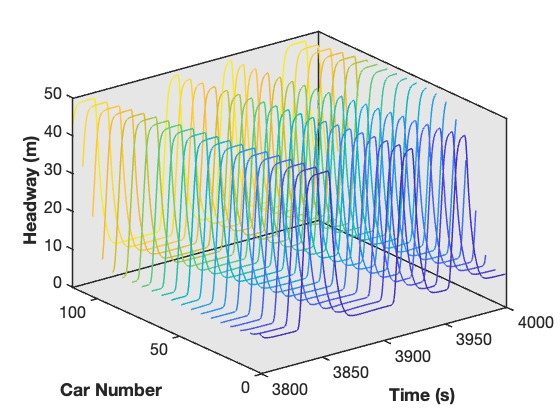
(a) $N=2$

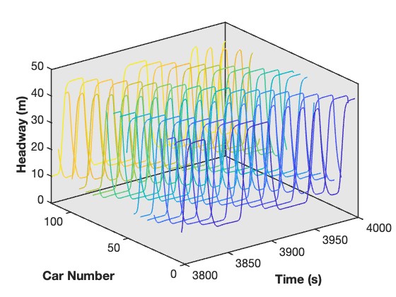
(b) $N=3$

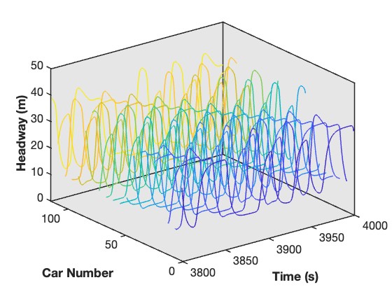
(c) $N=4$

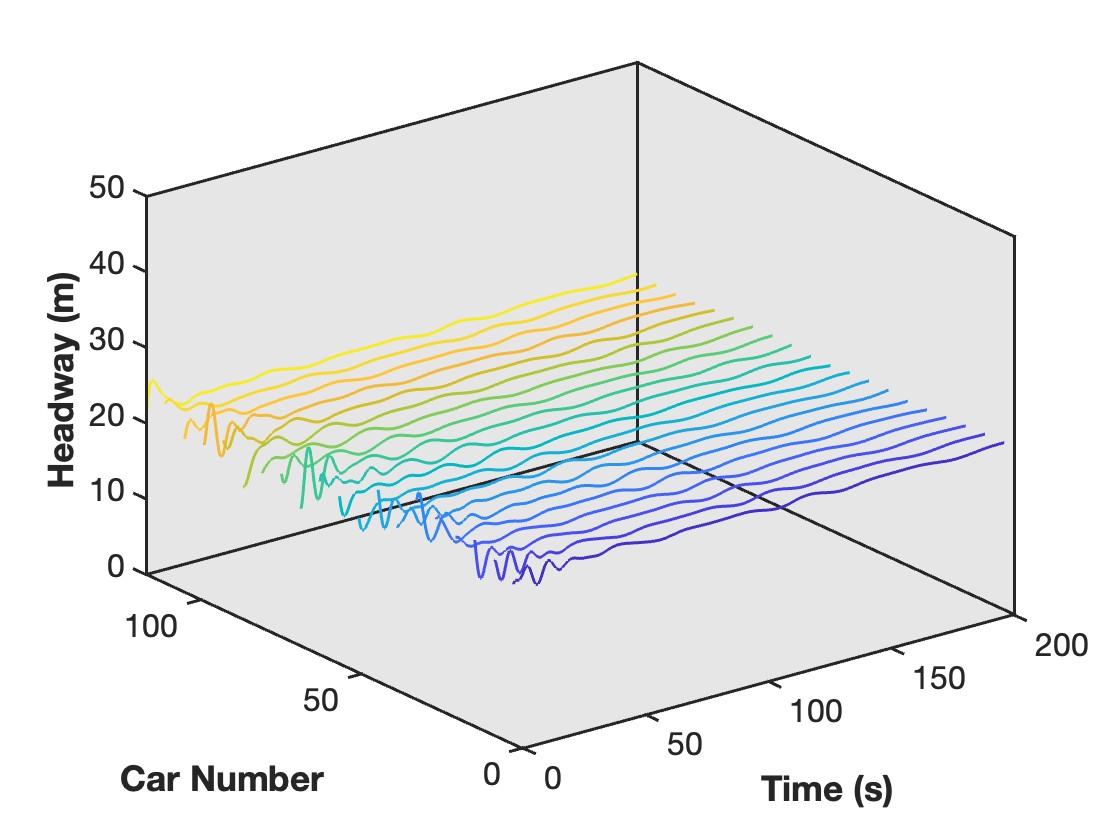
(d) $N=5$

Figure 8: Plots of headways for selected vehicles with no-connection for platoon sizes $N=2,3,4,5$.

Remark 5.

For the headway plots in this section, if the vehicles have not stabilized after $4000$s, we select every 6th vehicle from the 1st to the 120th for plotting, with the time interval spanning from 3800 to 4000 seconds. If the vehicles have stabilized, the headway plots will instead cover the time period from 0s until stabilization (60, 200, or 300s, depending on the scenario).

Figure 9 is the plots of minimum and maximum speeds of all vehicles corresponding to Figure 8.

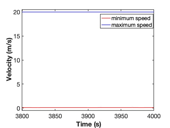
(a) $N=2$

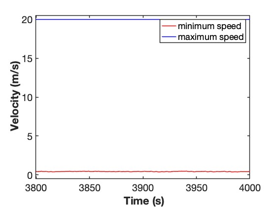
(b) $N=3$

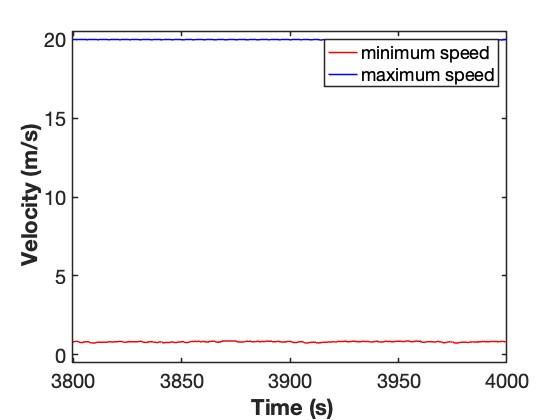
(c) $N=4$

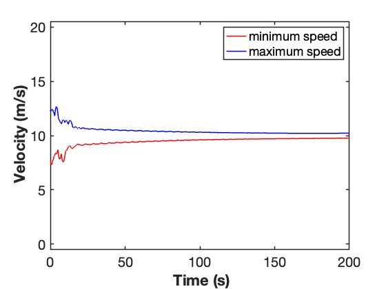
(d) $N=5$

Figure 9: Plots of minimum and maximum speeds of platoons with no-connection and size $N=2,3,4,5$.

Figure 10 is the headway plots for front-connected platoons of size $N=2,3,4$ and for two-way connected platoons of size $N=2$.

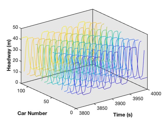
(a) $N=2$ front

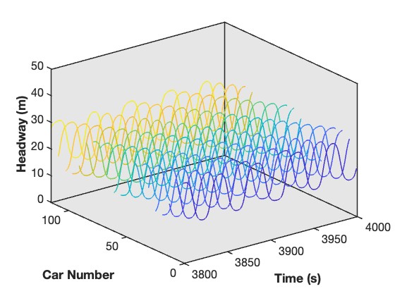
(b) $N=3$ front

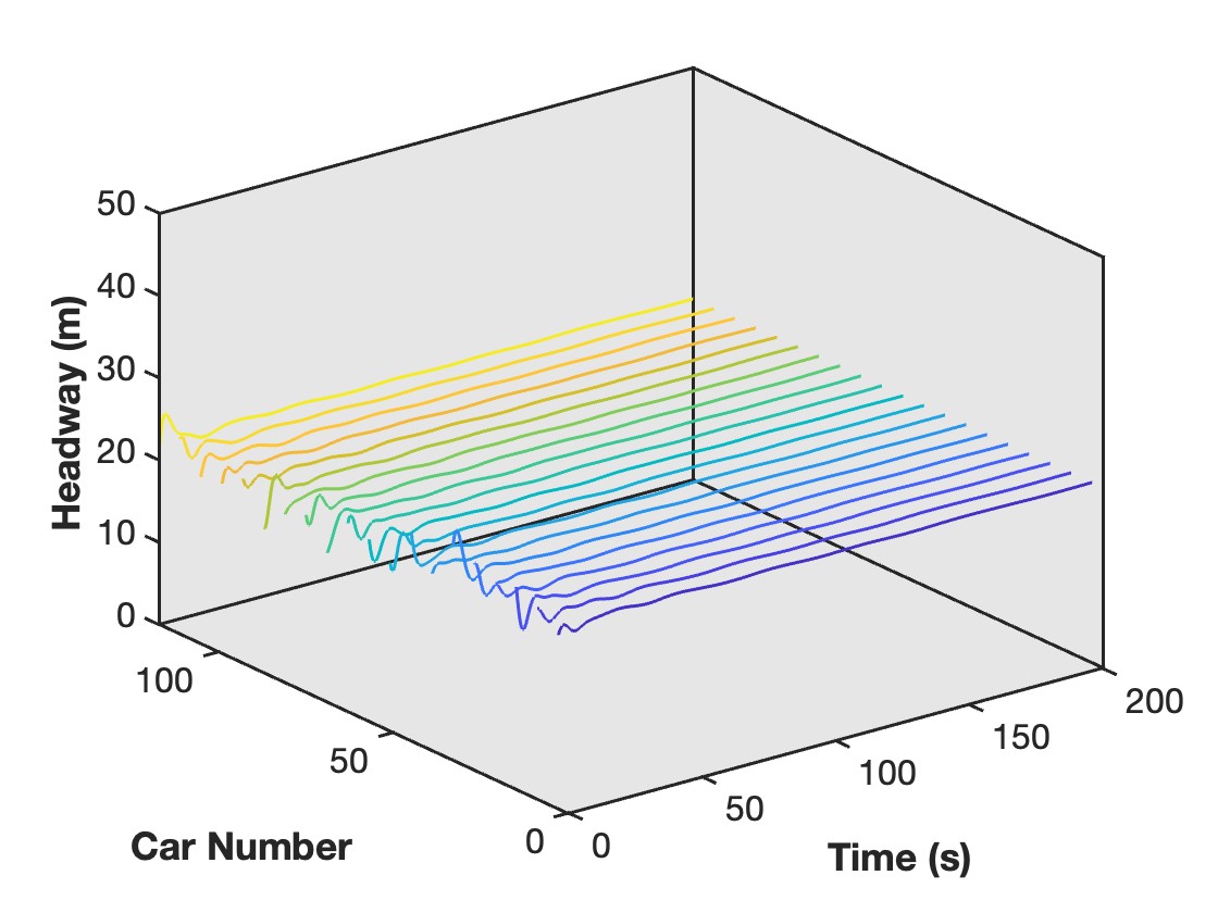
(c) $N=4$ front

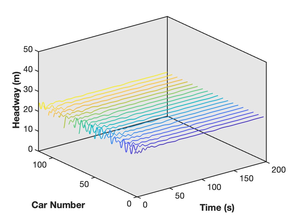
(d) $N=2$ two-way

Figure 10: Plots of headways for selected vehicles with front connection for platoon sizes $N=2,3,4$, two-way connection for platoon size $N=2$.

From the simulation results, we observe that stability of CAV platoons can be improved by increasing both platoon size and connectivity. Moreover, with two-way connections, the equilibrium state can be achieved with platoons consisting of just two CAVs. However, this condition is only guaranteed if the intra-platoon connections are robust and the inter-platoon communication is without delay.

IV-B2 Fixed platoon size with different delays

In this simulation, we aim to find the effects of inter-platoon communication delay. We fix the platoon size at $N=4$ and select different constant delays for both the front-connected model and two-way connected model. Figure 11 is the headway plots for the two-way connected model with communication delays $t_{d}=0.4,0.8,1.2,1.6$s.

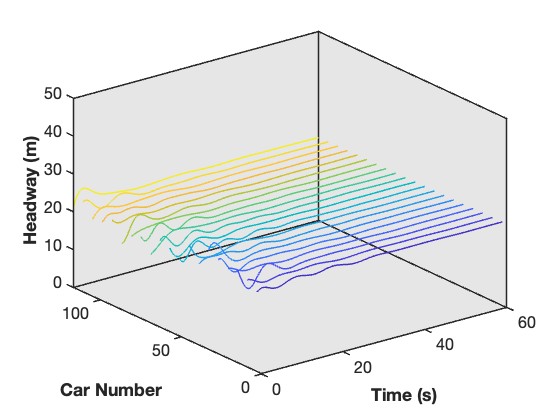
(a) $t_{d}=0.4$s

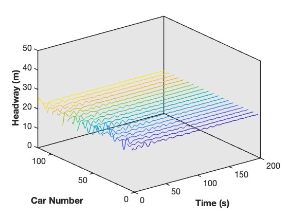
(b) $t_{d}=0.8$s

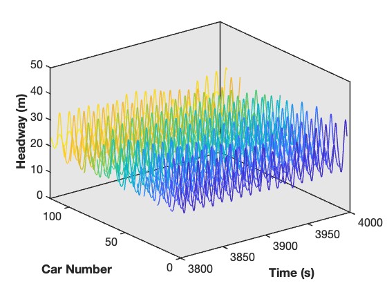
(c) $t_{d}=1.2$s

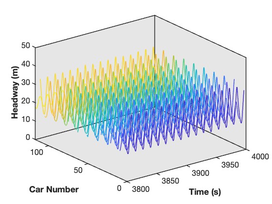
(d) $t_{d}=1.6$s

Figure 11: Plots of headways for selected vehicles with two-way connection for platoon size $N=4$ and communication delays $t_{d}=0.4,0.8,1.2,1.6$s.

Figure 12 is the plots of minimum and maximum speeds of all vehicles corresponding to Figure 11.

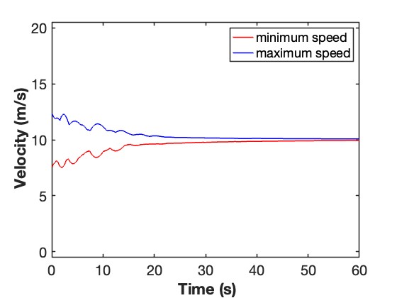
(a) $t_{d}=0.4$s

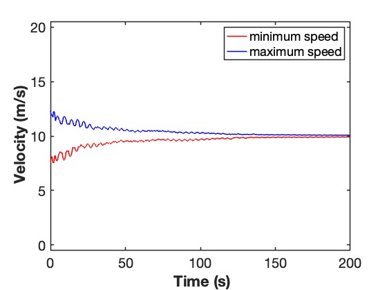
(b) $t_{d}=0.8$s

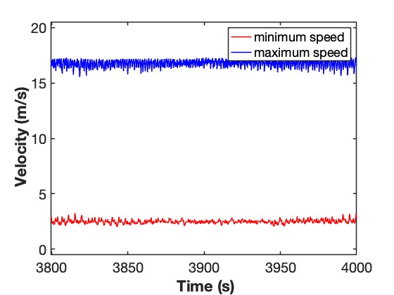
(c) $t_{d}=1.2$s

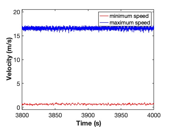
(d) $t_{d}=1.6$s

Figure 12: Plots of minimum and maximum speeds of platoons with no-connection of size $N=4$ and communication delays $t_{d}=0.4,0.8,1.2,1.6$s.

From the simulation results, we observe that increasing communication delays between platoons negatively impacts the stability of CAV platoons. Moreover, the variance in headways grows exponentially with increased delay, which aligns with theoretical analysis. These findings can guide CAV manufacturers in setting standards for sensors and other hardware components that influence communication delays.

IV-C Experiments of CAV platoons mixed with HDVs

One potential benefit of implementing CAV platoons in traffic flow is their stabilizing effect when mixed with HDVs (which can be treated as CAV platoons of size 1 with no communication). In this subsection, we test various distributions of CAV platoons and HDVs on the ring road described in Subsection IV-A to evaluate their impact on traffic flow stability.

IV-C1 Segregated CAV platoons and HDVs

We first consider the scenario where CAV platoons and HDVs are segregated into two distinct groups, each forming its own string of vehicles. The platoon configurations are set with sizes of $N=6$ or $N=8$, with no inter-platoon connections. Figure 13 is the headway plots for segregated traffic with CAV platoons of size $N=6$ with either $24$ or $30$ HDVs, and CAV platoons of size $N=8$ with either $32$ or $40$ HDVs.

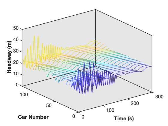
(a) $N=6$; $24$ HDVs

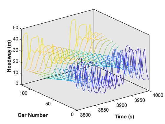
(b) $N=6$; $30$ HDVs

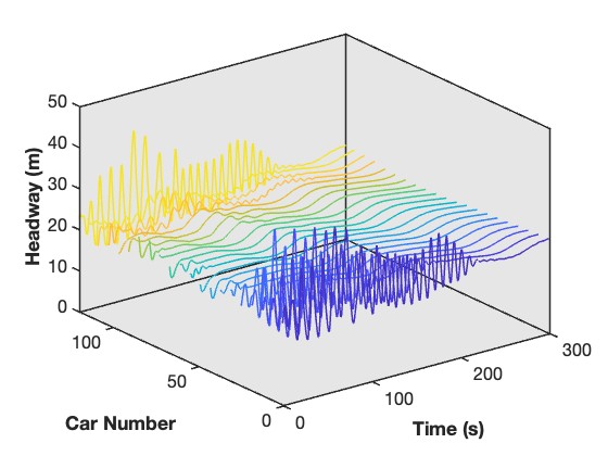
(c) $N=8$; $32$ HDVs

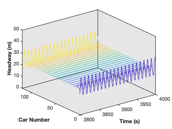
(d) $N=8$; $40$ HDVs

Figure 13: Headway plots for segregated traffic with CAV platoons of size $N=6$ with $30$ and $36$ HDVs and CAV platoons of size $N=8$ with $32$ and $40$ HDVs.

From this simulation, we observe that platoons of size $N=6$ can stabilize up to $30$ HDVs, slightly less than $32$ HDVs stabilized by platoons of size $N=8$.(It is worth noting that with 40 HDVs, the traffic flow is nearly stable.) Moreover, if the model does not reach equilibrium, the speed variation of HDVs is smaller when they are positioned closer to the tail CAV of the platoons, suggesting that HDVs are also prone to string instability.

IV-C2 Evenly mixed CAV platoons and HDVs

Another appraoch to distributing the vehicles is to mix CAV platoons and HDVs as evenly as possible, i.e. each platoon is follow by a fixed number of HDVs. We again assume that the CAV platoons are not connected, as the distance between platoon leaders is longer than flows of only CAV platoons, which could result in increased delays. Figure 14 is the headway plots for evenly mixed traffic, where CAV platoons of size $N=6$ are followed by $2$ or $3$ HDVs, and CAV platoons of size $N=8$ are followed by $5$ or $6$ HDVs.

Remark 6.

One of the platoons may be followed by a different number of HDVs to balance the distribution.

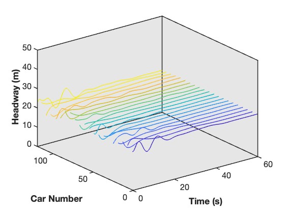
(a) $N=6$; $2$ HDV followers

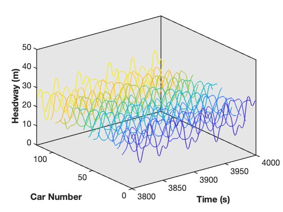
(b) $N=6$; $3$ HDV followers

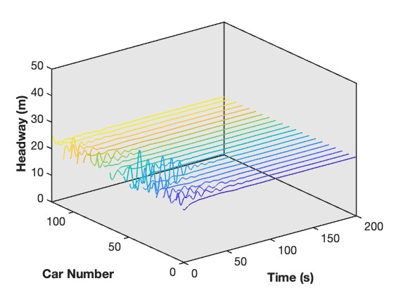
(c) $N=8$; $5$ HDV followers

(d) $N=8$; $6$ HDV followers

Figure 14: Headway plots for evenly mixed traffic with each CAV platoon of size $N=6$ followed by $2$ or $3$ HDVs, and CAV platoon of size $N=8$ followed by $5$ or $6$ HDVs.

From this simulation, we observed that in evenly mixed distributions, platoons of size $N=6$ can stabilize up to $30$ HDVs, while platoons of size $N=8$ can stabilize up to $48$ HDVs. This suggests that larger platoons act as more effective controllers of traffic stability. However, in scenarios with segregated distributions of $N=8$ with $40$ HDVs, the traffic flow is nearly stable, indicating that the improvements provided by the even distribution are relatively minor. where stability is not fully achieved, the speed variation among HDVs decreases more significantly when they are positioned closer to the platoons, consistent with previous observations.

V Conclusions

In this paper, we have extended a recently proposed single platoon CF model to accommodate multiple platoons. By treating the leading vehicle of each platoon considered as control inputs, we developed two distinct control designs that account for varying degrees of connectivity between platoons. We showed that our proposed multi-platoon models are consistent with foundational car-following models when the platoon size is reduced to $1$.

Through linear stability analysis, we demonstrated that both platoon size and the level of inter-platoon communication can enhance system stability. The results of numerical experiments with varied platoon size and connectivity are consistent with theoretical analysis. Furthermore, when testing configurations that mixed CAV platoons with HDVs, we observed that HDVs benefit from following CAV platoons—even without specific design considerations for HDV control.

A notable outcome of our analysis is that the influence of inter-platoon connections diminishes as platoon sizes increase. This suggests that, from a manufacturing standpoint, enhancing V2V communication within platoons should be prioritized over V2I communications. Another finding is that the stability of mixed traffic flow exhibits similar characteristics in scenarios where CAV platoons are either evenly distributed or segregated—a result that consists with a study of macroscopic models of mixed flow [45].

This paper provides a solid foundation for future innovations in CAV technologies and opens several avenues for further exploration. Integration with other control strategies, such as feedback and optimal control, could significantly enhance stability, safety, and comfort for travelers. Additionally, addressing fairness within the model and considering dynamic leader switching and platoon reformation could lead to more practical and equitable applications. Extending the proposed platoon models to accommodate more complex traffic scenarios, such as multi-lane roads and signalized intersections, would broaden the models’ applicability.

Shouwei Hui received the B.S. degree in applied mathematics from Shanghai Jiaotong University, and the M.A. degree in mathematics from the University of Wisconsin, Madison. He is currently pursuing the Ph.D. degree in applied mathematics at the University of California, Davis. His research interests include mathematical modelling, connected and autonomous vehicles, and intelligent transportation systems.

Michael Zhang received the B.S. degree in civil engineering from Tongji University, Shanghai, China, and the M.S. and Ph.D. degrees in engineering from the University of California, Irvine, Irvine, CA, USA. He is currently a Professor with the Civil and Environmental Engineering Department, University of California, Davis, Davis, CA, USA. His research interests include traffic operations and control, transportation network analysis, and intelligent transportation systems. He is also an Associate Editor of Transportation Research Part B: Methodological.

References

- [1] S. Sheikholeslam and C. A. Desoer, “Longitudinal control of a platoon of vehicles,” in 1990 American control conference. IEEE, 1990, pp. 291–296.
- [2] L. A. Pipes, “An operational analysis of traffic dynamics,” Journal of applied physics, vol. 24, no. 3, pp. 274–281, 1953.
- [3] M. Bando, K. Hasebe, A. Nakayama, A. Shibata, and Y. Sugiyama, “Dynamical model of traffic congestion and numerical simulation,” Physical review E, vol. 51, no. 2, p. 1035, 1995.
- [4] M. Bando, K. Hasebe, K. Nakanishi, A. Nakayama, A. Shibata, and Y. Sugiyama, “Phenomenological study of dynamical model of traffic flow,” Journal de Physique I, vol. 5, no. 11, pp. 1389–1399, 1995.
- [5] M. Treiber, A. Hennecke, and D. Helbing, “Congested traffic states in empirical observations and microscopic simulations,” Physical review E, vol. 62, no. 2, p. 1805, 2000.
- [6] R. Jiang, Q. Wu, and Z. Zhu, “Full velocity difference model for a car-following theory,” Physical Review E, vol. 64, no. 1, p. 017101, 2001.
- [7] S. Yu, Q. Liu, and X. Li, “Full velocity difference and acceleration model for a car-following theory,” Communications in Nonlinear Science and Numerical Simulation, vol. 18, no. 5, pp. 1229–1234, 2013.
- [8] O. Derbel, T. Peter, H. Zebiri, B. Mourllion, and M. Basset, “Modified intelligent driver model for driver safety and traffic stability improvement,” IFAC Proceedings Volumes, vol. 46, no. 21, pp. 744–749, 2013.
- [9] H. Lenz, C. Wagner, and R. Sollacher, “Multi-anticipative car-following model,” The European Physical Journal B-Condensed Matter and Complex Systems, vol. 7, pp. 331–335, 1999.
- [10] A. Nakayama, Y. Sugiyama, and K. Hasebe, “Effect of looking at the car that follows in an optimal velocity model of traffic flow,” Physical Review E, vol. 65, no. 1, p. 016112, 2001.
- [11] W.-X. Zhu and H. M. Zhang, “Analysis of mixed traffic flow with human-driving and autonomous cars based on car-following model,” Physica A: Statistical Mechanics and its Applications, vol. 496, pp. 274–285, 2018.
- [12] J. Wang, Y. Zheng, C. Chen, Q. Xu, and K. Li, “Leading cruise control in mixed traffic flow: System modeling, controllability, and string stability,” IEEE Transactions on Intelligent Transportation Systems, vol. 23, no. 8, pp. 12 861–12 876, 2021.
- [13] D. Jia and D. Ngoduy, “Platoon based cooperative driving model with consideration of realistic inter-vehicle communication,” Transportation Research Part C: Emerging Technologies, vol. 68, pp. 245–264, 2016.
- [14] J. Sun, Z. Zheng, and J. Sun, “The relationship between car following string instability and traffic oscillations in finite-sized platoons and its use in easing congestion via connected and automated vehicles with idm based controller,” Transportation Research Part B: Methodological, vol. 142, pp. 58–83, 2020.
- [15] L. Zhang, M. Zhang, J. Wang, X. Li, and W. Zhu, “Internet connected vehicle platoon system modeling and linear stability analysis,” Computer Communications, vol. 174, pp. 92–100, 2021.
- [16] Z. Zhou, L. Li, X. Qu, and B. Ran, “An autonomous platoon formation strategy to optimize cav car-following stability under periodic disturbance,” Physica A: Statistical Mechanics and its Applications, vol. 626, p. 129096, 2023.
- [17] ——, “A self-adaptive idm car-following strategy considering asymptotic stability and damping characteristics,” Physica A: Statistical Mechanics and its Applications, vol. 637, p. 129539, 2024.
- [18] S. Hui and M. Zhang, “A new platooning model for connected and autonomous vehicles to improve string stability,” arXiv preprint arXiv:2405.18791, 2024.
- [19] L. Davis, “Modifications of the optimal velocity traffic model to include delay due to driver reaction time,” Physica A: Statistical Mechanics and its Applications, vol. 319, pp. 557–567, 2003.
- [20] M. Treiber, A. Kesting, and D. Helbing, “Delays, inaccuracies and anticipation in microscopic traffic models,” Physica A: Statistical Mechanics and its Applications, vol. 360, no. 1, pp. 71–88, 2006.
- [21] C. Zhao, H. Yu, and T. G. Molnar, “Safety-critical traffic control by connected automated vehicles,” Transportation research part C: emerging technologies, vol. 154, p. 104230, 2023.
- [22] C. Zhao, T. G. Molnar, and H. Yu, “Leveraging cooperative connected automated vehicles for mixed traffic safety,” arXiv preprint arXiv:2406.11508, 2024.
- [23] Y. Jin and J. Meng, “Dynamical analysis of an optimal velocity model with time-delayed feedback control,” Communications in Nonlinear Science and Numerical Simulation, vol. 90, p. 105333, 2020.
- [24] A. Vahidi and A. Eskandarian, “Research advances in intelligent collision avoidance and adaptive cruise control,” IEEE transactions on intelligent transportation systems, vol. 4, no. 3, pp. 143–153, 2003.
- [25] V. Milanés, S. E. Shladover, J. Spring, C. Nowakowski, H. Kawazoe, and M. Nakamura, “Cooperative adaptive cruise control in real traffic situations,” IEEE Transactions on intelligent transportation systems, vol. 15, no. 1, pp. 296–305, 2013.
- [26] Y. Zheng, S. E. Li, J. Wang, D. Cao, and K. Li, “Stability and scalability of homogeneous vehicular platoon: Study on the influence of information flow topologies,” IEEE Transactions on intelligent transportation systems, vol. 17, no. 1, pp. 14–26, 2015.
- [27] Ş. Sabău, C. Oară, S. Warnick, and A. Jadbabaie, “Optimal distributed control for platooning via sparse coprime factorizations,” IEEE Transactions on Automatic Control, vol. 62, no. 1, pp. 305–320, 2016.
- [28] B. Besselink and K. H. Johansson, “String stability and a delay-based spacing policy for vehicle platoons subject to disturbances,” IEEE Transactions on Automatic Control, vol. 62, no. 9, pp. 4376–4391, 2017.
- [29] F. Gao, S. E. Li, Y. Zheng, and D. Kum, “Robust control of heterogeneous vehicular platoon with uncertain dynamics and communication delay,” IET Intelligent Transport Systems, vol. 10, no. 7, pp. 503–513, 2016.
- [30] W. Yu, X. Hua, D. Ngoduy, and W. Wang, “On the assessment of the dynamic platoon and information flow topology on mixed traffic flow under connected environment,” Transportation research part C: emerging technologies, vol. 154, p. 104265, 2023.
- [31] W. Yu, D. Ngoduy, X. Hua, and W. Wang, “On the stability of a heterogeneous platoon-based traffic system with multiple anticipations in the presence of connected and automated vehicles,” Transportation Research Part C: Emerging Technologies, vol. 157, p. 104389, 2023.
- [32] Y. Zhou, M. Wang, and S. Ahn, “Distributed model predictive control approach for cooperative car-following with guaranteed local and string stability,” Transportation research part B: methodological, vol. 128, pp. 69–86, 2019.
- [33] S. Graffione, C. Bersani, R. Sacile, and E. Zero, “Model predictive control of a vehicle platoon,” in 2020 IEEE 15th International Conference of System of Systems Engineering (SoSE). IEEE, 2020, pp. 513–518.
- [34] Y. Li, Q. Lv, H. Zhu, H. Li, H. Li, S. Hu, S. Yu, and Y. Wang, “Variable time headway policy based platoon control for heterogeneous connected vehicles with external disturbances,” IEEE Transactions on Intelligent Transportation Systems, vol. 23, no. 11, pp. 21 190–21 200, 2022.
- [35] T. Liu, L. Lei, K. Zheng, and K. Zhang, “Autonomous platoon control with integrated deep reinforcement learning and dynamic programming,” IEEE Internet of Things Journal, vol. 10, no. 6, pp. 5476–5489, 2022.
- [36] B. Li, “Stochastic modeling for vehicle platoons (i): Dynamic grouping behavior and online platoon recognition,” Transportation Research Part B: Methodological, vol. 95, pp. 364–377, 2017.
- [37] ——, “Stochastic modeling for vehicle platoons (ii): Statistical characteristics,” Transportation Research Part B: Methodological, vol. 95, pp. 378–393, 2017.
- [38] R. E. Stern, S. Cui, M. L. Delle Monache, R. Bhadani, M. Bunting, M. Churchill, N. Hamilton, H. Pohlmann, F. Wu, B. Piccoli et al., “Dissipation of stop-and-go waves via control of autonomous vehicles: Field experiments,” Transportation Research Part C: Emerging Technologies, vol. 89, pp. 205–221, 2018.
- [39] S. Tsugawa, S. Kato, and K. Aoki, “An automated truck platoon for energy saving,” in 2011 IEEE/RSJ international conference on intelligent robots and systems. IEEE, 2011, pp. 4109–4114.
- [40] J. W. Lee, H. Wang, K. Jang, A. Hayat, M. Bunting, A. Alanqary, W. Barbour, Z. Fu, X. Gong, G. Gunter et al., “Traffic control via connected and automated vehicles: An open-road field experiment with 100 cavs,” arXiv preprint arXiv:2402.17043, 2024.
- [41] S.-T. Zheng, R. Jiang, J. Tian, X. Li, B. Jia, Z. Gao, and S. Yu, “A comparison study on the growth pattern of traffic oscillations in car-following experiments,” Transportmetrica B: Transport Dynamics, vol. 11, no. 1, pp. 706–724, 2023.
- [42] S. Zhou, J. Tian, Y.-E. Ge, S. Yu, and R. Jiang, “Experimental features of emissions and fuel consumption in a car-following platoon,” Transportation Research Part D: Transport and Environment, vol. 121, p. 103823, 2023.
- [43] J. Zhou, Z.-K. Shi, and J.-L. Cao, “Nonlinear analysis of the optimal velocity difference model with reaction-time delay,” Physica A: Statistical Mechanics and its Applications, vol. 396, pp. 77–87, 2014.
- [44] D. Ngoduy, “Linear stability of a generalized multi-anticipative car following model with time delays,” Communications in Nonlinear Science and Numerical Simulation, vol. 22, no. 1-3, pp. 420–426, 2015.
- [45] S. Hui and M. Zhang, “An anisotropic traffic flow model with look-ahead effect for mixed autonomy traffic,” arXiv preprint arXiv:2407.20554, 2024.