Average Distance of Random Bipartite Matching in Discrete Networks

Abstract

The bipartite matching problem is widely applied in the field of transportation; e.g., to find optimal matches between supply and demand over time and space. Recent efforts have been made on developing analytical formulas to estimate the expected matching distance in bipartite matching with randomly distributed vertices in two- or higher-dimensional spaces, but no accurate formulas currently exist for one-dimensional problems. This paper presents a set of closed-form formulas, without curve-fitting, that can provide accurate average distance estimates for one-dimensional random bipartite matching problems (RBMP). We first focus on one-dimensional space and propose a new method that relates the corresponding matching distance to the area size between a random walk path and the x-axis. This result directly leads to a straightforward closed-form formula for balanced RBMPs. For unbalanced RBMPs, we first analyze the properties of an unbalanced random walk that can be related to balanced RBPMs after optimally removing a subset of unmatched points, and then derive a set of approximate formulas. Additionally, we build upon an optimal point removal strategy to derive a set of recursive formulas that can provide more accurate estimates. Then, we shift our focus to regular discrete networks, and use the one-dimensional results as building blocks to derive RBMP formulas. To verify the accuracy of the proposed formulas, a set of Monte-Carlo simulations are generated for a variety of matching problems settings. Results indicate that our proposed formulas provide quite accurate distance estimations for one-dimensional line segments and discrete networks under a variety of conditions.

1 Introduction

The bipartite matching problem (Asratian et al.,, 1998) is defined on a bipartite graph, in which vertices are divided into two disjoint subsets and edges only exist between vertices from different subsets. The objective is to identify an optimal subset of edges that match the vertices into disjoint pairs. The problem has diverse applications across many science and engineering fields. In biology, it can be used to measure and analyze the similarity between heterogeneous genes (Zhang et al.,, 2014), or to examine the structural relationship between proteins (Wang et al.,, 2004). In robotics, it can be applied to efficiently allocate tasks among multiple decentralized robots (Ghassemi and Chowdhury,, 2018), or to design coordination mechanisms to prevent collisions along paths of multiple agents (Dutta and Dasgupta,, 2017). In computer science, it can be used to find optimal allocation of virtual machines to users, so as to reduce delay in mobile cloud computing (Jin et al.,, 2022).

In the field of transportation, bipartite matching problems are widely applicable; e.g., to find optimal matches between supply and demand points over continuous time and space. For example, in two-dimensional spaces, it can be used to model how surface vehicles (e.g., taxi) are matched to their customers, such as in ride-hailing or food delivery systems (Shen et al.,, 2024; Tafreshian and Masoud,, 2020). In three-dimensional spaces, it can be used to dynamically dispatch and reposition aerial vehicles (drones) for delivering goods in the air (Aloqaily et al.,, 2022), or to optimize the flying trajectories of drone swarms during take-off and landing (Hernández et al.,, 2021). In addition, bipartite matches that span the time dimension can be useful for finding the optimal schedules among a series of tasks (Ding et al.,, 2021; Afèche et al.,, 2022), such as optimizing container transshipment among freight trains (Fedtke and Boysen,, 2017), or minimizing customer/vehicle waiting in reservation-based ride-sharing services (Shen and Ouyang,, 2023).

Strictly speaking, bipartite matching applications in the transportation field are likely to be associated with a sparse discrete network, where supply and demand points are distributed along network edges (after ignoring the local access legs) (Abeywickrama et al.,, 2022). A special case would be one on one-dimensional transportation routes or corridors. For instance, it can be used to model the operations of drones that are used to deliver goods to customers located on different floors of a tall building (Ezaki et al.,, 2024; Seth et al.,, 2023), or vehicle-customer matching for a ride-hailing system on a single city corridor (Panigrahy et al.,, 2020).

Any bipartite matching problem instance can be solved very efficiently using a range of well-known algorithms, including combinatorial optimization algorithms such as Hungarian algorithm (Kuhn,, 1955) and Jonker-Volgenant algorithm (Jonker and Volgenant,, 1987), or newly developed machine-learning based algorithms (Georgiev and Liò,, 2020). However, in the context of service and resource planning, one is often interested in estimating the average matching cost across various problem realizations, so as to evaluate the service efficiency under and resource investments. For example, in designing mobility services, the average matching distance, often referred to as the “deadheading” distance, is a key indicator that captures the unproductive cost spent by both service vehicles (i.e., running without passengers) and customers (i.e., waiting for pickup). Analytical formulas that reveal the relationship between the average matching distance and vehicle/customer distribution, such as those developed in Daganzo, (1978) and Yang et al., (2010), are often preferred by the service operators, because these formulas can not only provide valuable managerial insights, but also be directly incorporated into mathematical models to optimize service offerings. Similar formulas have been used to design system-wide operational standards (e.g., demand pooling time interval) for customer-vehicle matching (Shen et al.,, 2024), evaluate the effectiveness of newly proposed customer matching strategies (Ouyang and Yang,, 2023; Shen and Ouyang,, 2023; Stiglic et al.,, 2015), or analyze the impacts of pricing and market competition on the social welfare (Wang et al.,, 2016; Zhou et al.,, 2022).

The need to estimate the expected bipartite matching distance for planning decisions has led to the exploration of a stochastic version of the problem, known as “Random Bipartite Matching Problem (RBMP)” in the literature. Earlier studies in the field of statistical physics were among the first to explore such a problem. Mezard and Parisi, (1985) used a “replica method” to derive asymptotic formulas for the average optimal cost of a matching problem where the numbers of points in both subsets are nearly equal (i.e., balanced), and the edge weights identically and independently follow a uniform distribution. Building upon this work, Caracciolo et al., (2014) developed asymptotic approximations for the average Euclidean matching distance for balanced RBMPs in spaces with a dimension higher than two. However, these asymptotic approximations were derived under the strong assumption that the number of bipartite vertices approaches infinity, and hence could only serve as bounds rather than exact estimates when the number of vertices is small. More importantly, their proposed formulas require curve fitting that estimates coefficients from simulated data. Daganzo and Smilowitz, (2004) studied a related problem, which they call the Transportation Linear Programming (TLP), and proposed approximated formula for estimating the average item-distance among points with normally distributed demands and supplies. Through probabilistic and dimensional analysis, they introduced a bound to estimate the solution in two- and higher dimensions. Very recently, Shen et al., (2024) proposed a set of closed-form formulas for arbitrary numbers of points in both subsets, an arbitrary number of spatial dimensions, and arbitrary Lebesgue distance metrics. Their model has shown to provide very accurate estimates, without curve fitting, in spaces with higher than two dimensions. However, their approach ignores the boundary of the space as well as the resulted correlation among the matched pairs, which is reasonable for higher dimension spaces but causes notable errors in one-dimensional space especially when the the two subsets are (nearly) of equal size.

For one-dimensional problems, Caracciolo et al., (2017) proposed an asymptotic formula for estimating the square of the average matching distance. However, similar to other asymptotic approximations, their formula is applicable only in a limited number of scenarios; e.g., when the number of bipartite vertices is balanced and approaches infinity. Also, their formula also require curve fitting based on simulated data. Meanwhile, Daganzo and Smilowitz, (2004) also proposed an exact formula for the average minimal item-distance among points with normally distributed demand and supply in a one-dimensional space. Their results cannot be directly applied to RBMP, because they assume that (i) the supply and demand points are balanced, and that (ii) the supply or demand value associated with each randomly distributed point follows a normal distribution, while in RBMP, these values are either positive one or negative one. Nevertheless, their analysis provides very strong insights. One of their key findings is that the total minimal item-distance for all points is equal to the size of the area enclosed by the cumulative supply curve and the x-axis. This essential property also holds for our one-dimensional RBMP.

To the best of our knowledge, no existing formula can provide accurate estimates for RBMPs (with arbitrary numbers of bipartite vertices) in a one-dimensional space or in a discrete network. This paper aims to to fill this gap by introducing a set of closed-form formulas (without curve-fitting) that can provide sufficiently accurate estimates. This is done in two steps. First, we estimate the expected optimal matching distance for one-dimensional RBMPs. Our proposed method relates the matching distance in a balanced RBMP to the enclosed area size between the path of a random walk and the x-axis, and derives a closed-form formula for the optimal matching distance for balanced RBMPs. For the more challenging unbalanced RBMPs, a closed-form approximate formula is developed by analyzing the properties of an unbalanced random walk and the optimal way to remove a subset of excessive points. Additionally, a feasible point removal and swapping process is proposed to develop a set of recursive formulas that are more accurate. Next, we study the scaling property of the expected optimal matching distance in arbitrary-length lines. The insights are used as building blocks to derive formulas for RBMPs on a discrete regular network, when all points are generated from spatial Poisson processes along the edges. The expected optimal matching distance is derived as the expectation across two probabilistic matching scenarios that a point may encounter: (i) the point is locally matched with a point on the same edge, or (ii) it is globally matched with a point on another edge. To verify the accuracy of proposed formulas, a set of Monte-Carlo simulations are conducted for a variety of matching problem settings, for both one-dimensional and network problems. The results indicate that our proposed formulas have very high accuracy in all experimented problem settings. The proposed distance estimates, in simple closed forms, could be directly used in mathematical programs for strategic performance evaluation and optimization.

The remainder of this paper is organized as follows. Section 2 below first presents models and formulas for one-dimensional RBMP (as a building block) in both balanced and unbalanced settings. Section 3 presents formulas for arbitrary-length lines, and then regular discrete networks. Section 4 then presents numerical experiments to validate the proposed formulas. Finally, Section 5 provides concluding remarks and suggests future research directions.

2 1D RBMP Distance Estimators

2.1 Problem Definition

We begin by defining the one-dimensional RBMP. Two sets of points, with given respective cardinalities $n\in\mathbb{Z}^{+}$ and $m\in\mathbb{Z}^{+}$, are independently and uniformly distributed on a unit-length line within $[0,1]$. Without loss of generality, we assume $n\geq m$. For each realization of the points’ locations, denote $V$ and $U$ as the two point sets, where $|V|=n$ and $|U|=m$. A bipartite graph can be constructed, whose set of edges $E$ connect every pair of points in the two sets; i.e., $E=\{(u,v):\operatorname{\forall}u\in U,v\in V\}$. The weight on edge $(u,v)\in E$ is the absolute difference between the two points’ coordinates $x_{u}$ and $x_{v}$, i.e., $\|x_{u}-x_{v}\|$. Since $n\geq m$, every point $u\in U$ can be matched with exactly one point $v\in V$. We let $y_{uv}=1$ if $u$ is matched to $v$, or $0$ otherwise. The objective is to find a set of matches $\{y_{uv}:\operatorname{\forall}u\in U,v\in V\}$ that minimize the total matching distance, as follows:

$$\min \sum_{u\in U,v\in V}y_{uv}\|x_{u}-x_{v}\|;$$ (1)

s.t. $$\sum_{v\in V}y_{uv}=1,\operatorname{\forall}u\in U;\quad\sum_{u\in U}y_{uv}\leq 1,\operatorname{\forall}v\in V;\quad y_{uv}\in\{0,1\},\operatorname{\forall}u\in U,v\in V.$$ (2)

The average optimal matching distance across the realized points in $U$ is a random variable which depends on the random realization of $U$ and $V$. Its distribution is clearly governed by parameters $m$ and $n$, and hence we denote it $X_{m,n}$. We are looking for a closed-form formula for the expectation of the average optimal matching distance, $\mathbb{E}[X_{m,n}]$. In order to do that, we first show that $X_{m,n}$ can be estimated based on the enclosed area between the path of a related random walk and the x-axis, and then we take expectation of this enclosed area. For a simple balanced problem (i.e. when $n=m$), we can directly derive a closed-form formula. For an unbalanced problem (when $n>m$), we first show optimality properties for the matching, and then build upon that to derive both a closed-form and a recursive formula.

2.2 Random walk approximation

For each realized instance of one-dimensional RBMP, let $I=U\cup V$. Sort all the points in $I$ by their x-coordinates between 0 and 1, and index them sequentially by $i$. For point $i\in I$, denote $x_{i}\in[0,1]$ as its x-coordinate and $z_{i}$ as the value of its supply; i.e., $z_{i}=1$ if $i\in V$ (indicating a supply point), or $z_{i}=-1$ if $i\in U$ (indicating a demand point). A cumulative “net” supply curve can then be constructed for any coordinate $x$ and any subset of points $I^{\prime}\subseteq I$; i.e., $S(x;I^{\prime})=\sum_{\{\operatorname{\forall}i\in I^{\prime},x_{i}\leq x\}}z_{i}$. It is clearly a piece-wise step function. There are three special cases: $S(x;I)$ represents the net supply curve constructed by the full set of points in $I$; $S(0;I^{\prime})$ and $S(1;I^{\prime})$ represent the net supply values at both ends of the curve, $x=0$ and $x=1$, respectively.

Every curve $S(x;I)$ can be related to the realized path of a specific type of one-dimensional random walk with $m+n$ steps, starting from $S(0;I)=0$. Among these $m+n$ steps, exactly $n$ steps each increase the net supply by $1$ and $m$ each decrease the net supply by $1$; as such $S(1;I)=n-m$. The locations of the points in $I$ correspond to the positions of these steps. Denote the distance (step size) from point (step) $i\in I$ to its next point (step) as $l_{i},\operatorname{\forall}i\in I\setminus\{|I|\}$. The step size varies because the points in $I$ are uniformly distributed along the x-axis.

Denote $A(x;I^{\prime})=\sum_{\{\operatorname{\forall}i\in I\setminus\{|I|\},x_{i}\leq x\}}l_{i}\cdot|S(x_{i};I^{\prime})|$ as the total absolute area between curve $S(x;I^{\prime})$ and the x-axis from 0 to $x$. For model simplicity, we assume the step sizes $l_{i},\operatorname{\forall}i\in I\setminus\{|I|\}$ are i.i.d., with mean $l$. Next we show how $\mathbb{E}[X_{m,n}]$ can be derived out of such an area, for both balanced and unbalanced matchings.

2.3 Balanced case ($m=n$)

We begin with the special case where $m=n$. Now set $I$ contains $2n$ points. Let $Y_{n}=A(1;I)$ be the random variable that equals the total absolute area between curve $S(x;I)$ and the x-axis from 0 to 1. Daganzo and Smilowitz, (2004) proved that $A(1;I)$ must equal the minimum total shipping distance of a one-dimensional TLP with equal number of supply and demand points, and thus it must also equal the minimum total matching distance of the corresponding one-dimensional RBMP instance. Thus, the expected optimal matching distance per point can be estimated by the following:

$$\mathbb{E}[X_{n,n}]=\frac{1}{n}\cdot\mathbb{E}[Y_{n}].$$ (3)

To further estimate $\mathbb{E}[Y_{n}]$, we first consider a simpler type of related random walk with a fixed step size of unit length. Let $B(n)$ denote the expected area between the path of such a random walk and the x-axis. Harel, (1993) has provided a formula for $B(n)$, as follows:

$$B(n)=\frac{n2^{2n-1}}{\binom{2n}{n}}\xrightarrow{n\gg 1}\frac{n\sqrt{\pi n}}{2}.$$ (4)

The last step of approximation, when $n\gg 1$, comes from Stirling’s approximation. The basic intuition behind this formula is as follows. In a random walk with a fixed total number of steps (e.g., $2n$), there are a finite number of possible combinations of upward (e.g., $n+k$) steps and downward steps (e.g., $n-k$), when $k$ varies from 0 to $2n$. Next, for each $k$ value, the probability and expected area of a random walk can be determined: the probability is derived using backwards induction starting from some simple cases (e.g., $k=0$); the expected area, conditional on $k$, is computed by the absolute difference between the numbers of upward and downward steps, multiplied by the step size. (For example, for a random walk with $n+k$ upward steps and $n-k$ downward steps, its expected area between the curve and the x-axis can be show to be simply $2k$.) Then, Equation (4) can be obtained by taking the unconditional expectation of these area sizes across all possible values of $k$.

Then, consider the type of random walk with varying step sizes. Under the i.i.d. assumption for $l_{i}$, we can multiply $B(n)$ by the mean step size $l$ to obtain an approximate estimation for $\mathbb{E}[Y_{n}]$, as follows:

$$\mathbb{E}[Y_{n}]\approx l\cdot B(n).$$ (5)

Finally, according to Equations (3)-(5), and note $l=\frac{1}{2n}$ in this case, we obtain the following closed-form formula for $\mathbb{E}[X_{n,n}]$:

$$\mathbb{E}[X_{n,n}]=\frac{l\cdot B(n)}{n}=\frac{1}{2n}\cdot\frac{2^{2n-1}}{\binom{2n}{n}}\xrightarrow{n\gg 1}\frac{1}{4}\sqrt{\frac{{\pi}}{n}}.$$ (6)

2.4 Unbalanced case ($n>m$)

Next, we consider the unbalanced case where $n>m$, for which $n-m$ supply points from $V$ will remain unmatched for each realization. Let $V’\subset V$ denote the set of these $n-m$ unmatched points. If we remove all points in $V^{\prime}$ from $V$, the problem will reduce to a balanced one with an equal number (i.e., $m$) of demand and supply points. As a result, the values on the net supply curve after point removal, $S(x;I\setminus V^{\prime})$, at $x=0$ and $x=1$ should both equal zero; i.e.,

$$S(0;I\setminus V^{\prime})=S(1;I\setminus V^{\prime})=0.$$ (7)

Figure 1 shows an example of how such point removal process affects the net supply curve along the entire x-axis. In this figure, the points in $V$ and $U$ are represented by the red dots and blue triangles, respectively. The original and post-removal curves, $S(x;I)$ and $S(x;I\setminus V^{\prime})$, are represented by the red dash-dot line and blue dashed line, respectively. The points in $V^{\prime}$ and the net supply values at their corresponding coordinates on the original curve, $S(x_{v^{\prime}};I),\operatorname{\forall}v^{\prime}\in V^{\prime}$, are marked by the black cross markers. Note that every time a point $v^{\prime}\in V^{\prime}$ is removed, the net supply values within $[x_{v^{\prime}},1]$ will decrease by one. As a result, the cumulative reduction of net supply at position $x$ should be determined by the total number of removed points within $[0,x]$. Sort the points in $V^{\prime}$ by their x-coordinates, from left to right, as $\{v^{\prime}_{1},\dots,v^{\prime}_{n-m}\}$. If we further denote $v^{\prime}_{0}$ and $v^{\prime}_{n-m+1}$ as two virtual points at the boundaries; i.e. $x_{v^{\prime}_{0}}=0$ and $x_{v^{\prime}_{n-m+1}}=1$, then the net supply values on the two curves within range $[x_{v^{\prime}_{k}},x_{v^{\prime}_{k+1}})$ must satisfy the following relationship:

$$S(x;I\setminus V^{\prime})=S(x;I)-k,\operatorname{\forall}k\in\{0,\cdots,n-m\},x\in[x_{v^{\prime}_{k}},x_{v^{\prime}_{k+1}}).$$ (8)

This relationship is illustrated in Figure 1 by the black arrows.

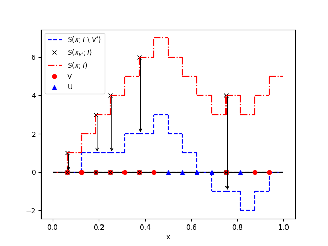
Figure 1: Point removal process in an unbalanced problem.

Among all possible combinations of points in set $V^{\prime}$, we denote $V^{*}$ as the optimal set of removed points that minimizes the area enclosed by the post-removal curve and the x-axis:

$$V^{*} =\operatorname*{argmin}_{\operatorname{\forall}V^{{}^{\prime}}\subset V,\text{ }|V^{{}^{\prime}}|=n-m}A(1;I\setminus V^{{}^{\prime}}).$$

The optimal post-removal area $A(1;I\setminus V^{*})$, enclosed by the optimal post-removal curve $S(1;I\setminus V^{*})$ and the x-axis, must equal the minimum total matching distance of the original unbalanced RBMP instance. Set random variable $Z_{m,n}=A(1;I\setminus V^{*})$ which depends on the random realization of $I=U\cup V$ (where $|V|=n$ and $|U|=m$), and then, similar to how we handle the balanced case:

$$\mathbb{E}[X_{m,n}]=\frac{1}{m}\cdot\mathbb{E}[Z_{m,n}].$$ (9)

In the following subsections, we will: (i) show the optimal post-removal curve must include a series of balanced random walk segments; (ii) derive an approximate closed-form formula for $\mathbb{E}[X_{m,n}]$ by estimating the area of each balanced segment; (iii) provide an alternative estimation for $\mathbb{E}[X_{m,n}]$ with a recursive formula based on a feasible point selection process; and (iv) refine both estimations with a correction term.

2.4.1 Property of the optimal removal

We first show a necessary condition for the removed points to be optimal: the $k$-th removed point must have a net supply value of $k$ on the original curve $S(x;I)$. This is stated in the following proposition.

Proposition 1.

$S(x_{v^{*}_{k}};I)=k,\operatorname{\forall}k\in\{1,\dots,n-m\}.$

Proof.

To show the proposition holds, it is sufficient to show the following claim is true: For any point $v^{\prime}_{k}\in V^{\prime}$, if $S(x_{v^{\prime}_{k}};I)<k$ or $S(x_{v^{\prime}_{k}};I)>k$, we can always swap a point in $V^{\prime}$ with another point in $V\setminus V^{\prime}$ to reduce $A(x;I\setminus V^{{}^{\prime}})$; hence, $V^{\prime}$ cannot be optimal.

We begin with the case when $S(x_{v^{\prime}_{k}};I)<k$. According to Equation (8), $v^{\prime}_{k}$ must have a negative net supply value on the post-removal curve; i.e., $S(x_{v^{\prime}_{k}};I\setminus V^{\prime})<0$. Figure 2 (a) shows an example point $v^{\prime}_{k}$ (indicated by the cross marker) in such a condition. A portion of the post-removal curve including the removal of this single point, is represented by the red dash-dot line. Now we may check the points in $I$ to the right hand side of $v^{\prime}_{k}$ along the x-axis, until we encounter another supply point $v\in V$. Such a supply point $v$ is guaranteed to be within $(x_{v^{\prime}_{k}},1]$, otherwise $S(1;I\setminus V^{\prime})\leq S(x_{v^{\prime}_{k}};I\setminus V^{\prime})<0$, which violates Equation (7).

Two cases may arise here for $v$. The first case is when $v\notin V^{\prime}$, as shown in Figure 2 (a). Since $v$ is the first supply point to the right of $v^{\prime}_{k}$, the points within $(x_{v^{\prime}_{k}},x_{v})$, if any, must all be demand points, as shown by the blue triangles in Figure 2 (a). As all demand points have negative supply values, the net supply values on the post-removal curve within $(x_{v^{\prime}_{k}},x_{v})$ must be no larger than $S(x_{v^{\prime}_{k}};I\setminus V^{\prime})$; i.e., for $x\in(x_{v^{\prime}_{k}},x_{v})$, $S(x;I\setminus V^{\prime})\leq S(x_{v^{\prime}_{k}};I\setminus V^{\prime})<0$. Now swap $v^{\prime}_{k}$ out of $V^{\prime}$, and swap $v$ in. Note here such a point swap would only affect the post-removal curve within $[x_{v^{\prime}_{k}},x_{v})$, and after the swap, the original post-removal curve, $S(x;I\setminus V^{\prime})$, will increase by one unit within $[x_{v^{\prime}_{k}},x_{v})$, while all the other parts remain the same. The area size under the curve is strictly reduced by the point swap, by an amount of $A(x;I\setminus V^{{}^{\prime}})$, as shown by the gray area in Figure 2 (a). The reduced area size is:

$$\sum_{\{\operatorname{\forall}i\in I,x_{v^{\prime}_{k}}\leq x_{i}<x_{v}\}}l_{i}\cdot|S(x_{i};I\setminus V^{\prime}\setminus\{v\}\cup\{v^{\prime}_{k}\})-S(x_{i};I\setminus V^{\prime})|=\sum_{\{\operatorname{\forall}i\in I,x_{v^{\prime}_{k}}\leq x_{i}<x_{v}\}}l_{i}>0,$$

The last inequality holds because $v$ must exist. Therefore, the claim is true for $S(x_{v^{\prime}_{k}};I)<k$ (i.e., $S(x_{v^{\prime}_{k}};I\setminus V^{\prime})<0$) and $v\notin V^{\prime}$.

The other case occurs when $v\in V^{\prime}$. Since $v$ is the first supply point encountered in $V^{\prime}$ to the right of $v^{\prime}_{k}$, $v$ must be $v^{\prime}_{k+1}$. Again, all points within $(x_{v^{\prime}_{k}},x_{v})$, if any, must be demand points. In addition, since $v^{\prime}_{k+1}$ itself is a removed point, $S(x_{v^{\prime}_{k+1}};I\setminus V^{\prime})\leq S(x_{v^{\prime}_{k}};I\setminus V^{\prime})<0$. Then, we may simply change our focus from $v^{\prime}_{k}$ to $v^{\prime}_{k+1}$, and then scanning the points on the right side of $v^{\prime}_{k+1}$, and continue until we find a point $v^{\prime}\in V^{\prime}$ with $S(x_{v^{\prime}};I\setminus V^{\prime})<0$, and its next supply point $v\notin V^{\prime}$. The proof for the previous case would apply for swapping $v^{\prime}$ and $v$. Hence, the claim is also true for $S(x_{v^{\prime}_{k}};I)<k$ and $v\in V^{\prime}$.

When $S(x_{v^{\prime}_{k}};I)>k$, the proof is symmetric. We look for points to swap that can lead to area reduction for $A(x;I\setminus V^{{}^{\prime}})$ to the “left” hand side of $v^{\prime}_{k}$ along the x-axis, instead of the right. According to Equation (8), $v^{\prime}_{k}$ now must have a positive net supply value on the post-removal curve; i.e., $S(x_{v^{\prime}_{k}};I\setminus V^{\prime})>0$. A supply point to the left must exist within $[0,x_{v^{\prime}_{k}})$, or otherwise $S(0;I\setminus V^{\prime})\geq S(x_{v^{\prime}_{k}};I\setminus V^{\prime})>0$, which violates Equation (7). There are two similar cases here depending on whether $v$ is or is not in $V^{\prime}$. The logic of the proof is exactly symmetrical. The only difference is that, after swapping the two points, the original curve will “decrease” by one unit, instead of increase, within the interval. The area reduction is still strictly greater than zero, as shown in Figure 2 (b).

We have shown that the claim is true in all possible conditions. This indicates that if any removed point $v^{\prime}$ in an arbitrary set $V^{\prime}$ does not satisfy $S(x_{v^{\prime}_{k}};I)=k$, then $V^{\prime}$ cannot be optimal. Therefore, for any removed point $v^{*}_{k}$ in an optimal set $V^{*}$, $S(x_{v^{*}_{k}};I)=k$ must hold necessarily. This completes the proof.

∎

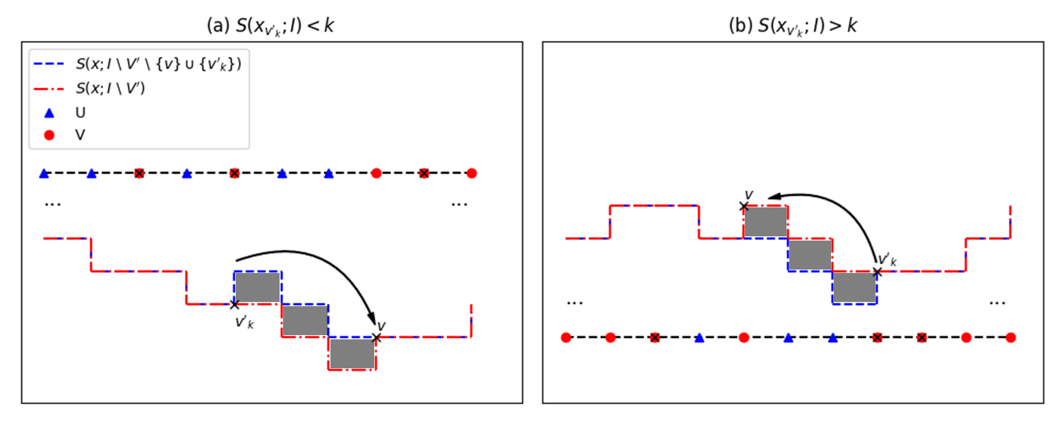
Figure 2: Illustration of the point swap process

Next, we present a useful property of the post-removal curve satisfying the optimality condition: $S(x_{v^{\prime}_{k}};I)=k,\operatorname{\forall}k\in\{1,\dots,n-m\}$. According to Equation (8), the net supply values on the post-removal curve at the locations of all removed points must be zero; i.e.: $S(x_{v^{\prime}_{k}};I\setminus V^{\prime})=S(x_{v^{\prime}_{k}};I)-k=0$. As such, the following proposition must hold.

Proposition 2.

For any given $V^{\prime}$, if $S(x_{v^{\prime}_{k}};I)=k,\operatorname{\forall}k\in\{0,1,\dots,n-m\}$, then each segment of the post-removal curve, $S(x;I\setminus V^{\prime})$ within $(x_{v^{\prime}_{k}},x_{v^{\prime}_{k+1}})$, can be regarded as the realized path of a corresponding balanced random walk.

2.4.2 An approximate closed-form formula

Propositions 1 and 2 show that the optimal post-removal curve $S(x;I\setminus V^{*})$ contains $n-m+1$ segments with end points $\{x_{v^{*}_{k}}\}_{k=0,1,\cdots}$, and each segment $(x_{v^{*}_{k}},x_{v^{*}_{k+1}})$ can be regarded as a realized path of a balanced random walk. Accordingly, we can decompose the optimal post-removal area $A(1;I\setminus V^{*})$ into $n-m+1$ segments as follows:

$$A(1;I\setminus V^{*})=\sum_{k=0}^{n-m}\left[A(x_{v^{*}_{k+1}};I\setminus V^{*})-A(x_{v^{*}_{k}};I\setminus V^{*})\right],$$ (10)

where each term $A(x_{v^{*}_{k+1}};I\setminus V^{*})-A(x_{v^{*}_{k}};I\setminus V^{*})$ represents the area of a balanced random walk segment within range $(x_{v^{*}_{k}},x_{v^{*}_{k+1}})$.

For model convenience, we again ignore the impact of boundaries and assume that every point $v\in V$ is probabilistically identical and independent to be selected in $V^{*}$. Based on this assumption, we can directly apply Equation (5) to estimate the expected area of each balanced random walk segment, which shall be dependent on only the number of (balanced) points and the mean step size within each segment. Denoting $m_{k}$ as the number of demand (or supply points) in $U$ in the $k$-th segment, $\mathbb{E}[Z_{m,n}]$ can then be approximately estimated as the following sum:

$$\mathbb{E}[Z_{m,n}]\approx\sum_{k=0}^{n-m}\mathbb{E}\left[l\cdot B(m_{k})\right].$$ (11)

It is approximate because: (i) we simply treat the the mean step size in each balanced random walk segment as the same as that of the original unbalanced random walk; i.e., $l=\frac{1}{n+m}$. This could lead to an overestimation, and a correction term could be added, as discussed in Section 2.4.4; (ii) with our i.i.d. assumption for $V^{*}$ and disregard of the boundary effects, we must have $m_{k},\operatorname{\forall}k\in\{0,\dots,n-m\}$ to be i.i.d. This may result in an underestimation, because points at specific positions may have a higher probability of being selected in $V^{*}$ than others due to the presence of boundaries.

Then, we may only focus on the expected area of the first segment; i.e., when $k=0$. Let $\text{Pr}\{m_{0}=m^{\prime}\}$ denote the probability that the first segment contains exactly $m^{\prime}\in\{1,\cdots,m\}$ demand points, noticing that the total number of demand points across all $n-m+1$ segments must equal $m$; i.e., $\sum_{k=0}^{n-m}m_{k}=m$. To derive $\text{Pr}\{m_{0}=m^{\prime}\}$ , one may relate it to the well-known “stars and bars” combinatorial problem. When we use $n-m$ “bars” (points in $V^{*}$) to partition $m$ stars (all matched pairs of demand and supply points), there are $\binom{n}{n-m}$ possible combinations for such a partition. Once the first segment has been set to contain $m^{\prime}$ stars, there remain $n-m^{\prime}-1$ positions for the remaining $n-m-1$ bars to be placed, resulting in $\binom{n-m^{\prime}-1}{n-m-1}$ possible combinations. That is,

$$\text{Pr}\{m_{0}=m^{\prime}\}=\frac{\binom{n-m^{\prime}-1}{n-m-1}}{\binom{n}{n-m}}.$$ (12)

Hence, following Equations (6), (9), and (12), and note $l=\frac{1}{n+m}$ in this case, we now have a closed-form formula for $\mathbb{E}[X_{m,n}]$, as follows:

$$\mathbb{E}[X_{m,n}] \approx(n-m+1)\cdot\mathbb{E}\left[l\cdot B(m_{0})\right]\approx(n-m+1)\cdot l\cdot\sum_{m^{\prime}=0}^{m}\text{Pr}\{m_{0}=m^{\prime}\}\cdot B(m^{\prime})$$

$$\approx\frac{n-m+1}{m(m+n)}\cdot\sum_{m^{\prime}=0}^{m}\frac{\binom{n-m^{\prime}-1}{n-m-1}}{\binom{n}{n-m}}\cdot\frac{m^{\prime}2^{2m^{\prime}-1}}{\binom{2m^{\prime}}{m^{\prime}}}.$$ (13)

Again, this formula is approximate due to our simplifying assumptions. In the next section, we will present an alternative method to yield a more accurate estimation via a specific point removal and swapping process.

2.4.3 Recursive formulas

In theory, the optimal point removal for each realization shall be solved as a dynamic program (and possibly via the Bellman equation); however, such an approach is not suitable for closed-form formulas. Therefore, this section builds upon Propositions 1 and 2 to propose a simpler point removal and swapping process that can yield a near-optimum point-removal solution for each realization. Then the area size estimation across realizations, based on this process, can be derived into a set of recursive formulas. The result provides a tight upper bound for $\mathbb{E}[X_{m,n}]$.

First, we propose a point removal process that is developed based on the necessary optimality conditions in Proposition 1, such that it provides a reasonably good (e.g., locally optimal) balanced random walk. We initialize $\hat{V}=\emptyset$ and $k=1$. Starting from $x=0$, scan the supply points in $V$ from left to right along the x-axis and check if a point satisfies the following conditions: (i) it has a net cumulative supply value of $k$; (ii) the nearest neighbor (in $I$) on the left, if existing, has a net supply value of $k-1$; and (iii) the net supply values of all points (in $I$) on the right hand side of this point is greater than or equal to $k$. If conditions (i)-(iii) are all satisfied by a point, denoted $\hat{v}_{k}$, then add it to the current set $\hat{V}$, increase $k$ by 1, and repeat the above procedure until $k=n-m$. The net supply values of the points selected in this procedure are guaranteed to form an increasing sequence; i.e.:

$$S(x_{\hat{v}_{k}};I)=k,\quad\operatorname{\forall}k\in\{1,\dots,n-m\}.$$

This is because, at step $k$ of the above process, the curve $S(x;I)$ must have a net supply value of $k-1$ at the previously selected point $\hat{v}_{k-1}$, and a value of at least $n-m$ at the final step at $x=1$. Hence, from intermediate value theorem, point $\hat{v}_{k}$ can always be found in $(x_{\hat{v}_{k-1}},1]$. Note that the removal of $\hat{v}_{k}$ at step $k$ only affects the curve on its right-hand side, with the segments on its left-hand side being balanced random walks. From the construction of the process, all points on the final post-removal curve $S(x;I\setminus\hat{V})$ surely have a non-negative net supply value; i.e.,

$$S(x;I\setminus\hat{V})\geq 0,\quad\operatorname{\forall}x\in(x_{\hat{v}_{k}},1],\text{ }k\in\{1,\cdots,n-m\}.$$

Figure 3 (a) shows a simple example of the point removal process, with $n-m=2$. The original curve, $S(x;I)$, is represented by the red dash-dot line, and two selected removal points $\hat{v}_{1}$ and $\hat{v}_{2}$ are represented by the black cross markers. At step 1 and 2, the removal of $\hat{v}_{1}$ and $\hat{v}_{2}$ decrease the net supply values of points in the red and purple shaded regions, respectively.

Figure 3: Illustration of the point removal and swap procedure.

We again use the term “segment of the curve” but now refer to the post-removal curve $S(x;I\setminus\hat{V})$ within $(x_{\hat{v}_{k}},x_{\hat{v}_{k+1}})$ as the “$k$-th segment” (which must be balanced). From the perspective of each point $\hat{v}_{k}$, the post-removal area in $(x_{\hat{v}_{k}},1]$ includes those within the $k$-th segment and $(x_{\hat{v}_{k+1}},1]$, both of which depend on the length of the $k$-th segment. Let $\text{Pr}\{\hat{m}_{k}\mid a\}$ denote the probability for the $k$-th segment to contain $\hat{m}_{k}$ demand (or supply) points, when there are exactly $a$ demand points in $(x_{v_{k}},1]$. In the step to select $v_{k+1}$, there are $n-m-k$ supply points to be removed; thus, there are $a+n-m-k$ supply points in $(x_{v_{k+1}},1]$. That is, the original curve $S(x;I)$ starts from value $k$ at $\hat{v}_{k}$ and returns to $k$ after exactly $2\hat{m}_{k}$ steps, which occurs with probability

$$\binom{a}{\hat{m}_{k}}\binom{a+n-m-k}{\hat{m}_{k}}/\binom{2a+n-m-k}{2\hat{m}_{k}},$$

but never returns to value $k$ afterwards, with probability from the well-known Ballot’s theorem (Addario-Berry and Reed,, 2008):

$$\frac{n-m-k}{2a+n-m-k-2\hat{m_{k}}}.$$

As such, we have

$$\text{Pr}\{\hat{m}_{k}\mid a\}=\frac{\binom{a}{\hat{m}_{k}}\binom{a+n-m-k}{\hat{m}_{k}}}{\binom{2a+n-m-k}{2\hat{m}_{k}}}\cdot\frac{n-m-k}{2a+n-m-k-2\hat{m}_{k}}.$$ (14)

Let $\hat{Z}_{k,a}$ represent the area enclosed by the x-axis and the post-removal curve $S(x;I\setminus\hat{V})$ within $(x_{\hat{v}_{k}},1]$, which contains exactly $a$ demand points. From Equation (5), the expected areas size of the balanced random walk inside the $k$-th segment $(x_{\hat{v}_{k}},x_{\hat{v}_{k+1}})$ is simply:

$$l\cdot B(\hat{m}_{k}).$$

Hence, conditional on $\hat{m}_{k}$, we have

$$\mathbb{E}[\hat{Z}_{k,a}] =\sum_{m^{\prime}=0}^{a}\text{Pr}\{\hat{m}_{k}=m^{\prime}\mid a\}\cdot\left[l\cdot B(m^{\prime})+\mathbb{E}[\hat{Z}_{k+1,a-m^{\prime}}]\right],$$

$$\operatorname{\forall}k\in\{0,\dots,n-m-1\},\quad 0\leq a\leq m,$$ (15)

and when $k=m-n$,

$$\mathbb{E}[\hat{Z}_{n-m,a}]=l\cdot B(a),\quad\operatorname{\forall}0\leq a\leq m.$$

When $k=0$, $\mathbb{E}[\hat{Z}_{0,m}]$ represents the expected area of the entire post-removal curve.

Next, we propose a refinement process based on local point swapping. It is intended to further reduce the post-removal area for a more accurate upper bound estimate. For all $k\in\{1,\dots,n-m-1\}$, if there exists a point $v\in V$ that satisfies (i) $x_{\hat{v}_{k}}<x_{v}<x_{\hat{v}_{k+1}}$, and (ii) $v$ is the nearest neighbour of $\hat{v}_{k}$ on the right, then we swap $\hat{v}_{k+1}$ out of set $\hat{V}$ and swap point $v$ in. We propose to perform exactly one such point swap to each of the segments.

An example of point swap is illustrated in Figure 3 (b). The post-removal curve $S(x;I\setminus\hat{V})$ is represented by the blue dash curves. After a swap between points $\hat{v}_{k+1}$ and $v$, the $k$-th curve segment will be shifted down by one unit (while all other segments remain the same), as indicated by the black dotted curves. Such a point swap can result in both reductions (if net supply $S(x;I\setminus\hat{V})>0$ before the swap, as the grey rectangles) and additions (if net supply $S(x;I\setminus\hat{V})=0$ before the swap, as the blue rectangles) to the enclosed area size. The following proposition says that the expected total area size will be reduced for each of the swaps. This indicates that the proposed point swapping process will yield a smaller (or at least equal) expected post-removal area size.

Suppose $\hat{m}_{k,0}\leq\hat{m}_{k}$ is the random number of points with zero net supplies within the $k$-th segment. According to the point swapping process, the area size reduction can be computed as the difference between the number of positive net-supply points, $2\hat{m}_{k}-\hat{m}_{k,0}$, and that of the zero net-supply points $\hat{m}_{k,0}$, multiplied by the expected step size $l$. If we take expectation of the area change with respect to $\hat{m}_{k,0}$, conditional on $\hat{m}_{k}$, we have

$$l\cdot\left(2\hat{m}_{k}-2\mathbb{E}[\hat{m}_{k,0}\mid\hat{m}_{k}]\right),\quad\operatorname{\forall}k\in\{1,\dots,n-m-1\}.$$ (16)

Note that to compute $\mathbb{E}[\hat{m}_{k,0}\mid\hat{m}_{k}]$, it is equivalent to compute the expected number of times a random walk with $2\hat{m}_{k}$ steps returns to zero. Clearly, this expectation equals zero when $\hat{m}_{k}=0$. Meanwhile, Harel, (1993) derived the probability that a random walk with $2\hat{m}_{k}$ steps returns to zero at the $2j$-th step, $\operatorname{\forall}j\in\{1,\dots,\hat{m}_{k}\}$:

$$\binom{2j-1}{j}\binom{2\hat{m}_{k}-2j}{\hat{m}_{k}-j}/\binom{2\hat{m}_{k}-1}{\hat{m}_{k}},\quad\operatorname{\forall}k\in\{1,\dots,n-m-1\}.$$

Summing these probabilities across all possible values of $j$, we have

$$\mathbb{E}[\hat{m}_{k,0}\mid\hat{m}_{k}]=\begin{cases}0,\quad&\operatorname{\forall}\hat{m}_{k}=0,\\ \sum_{j=1}^{\hat{m}_{k}}\binom{2j-1}{j}\binom{2\hat{m}_{k}-2j}{\hat{m}_{k}-j}/\binom{2\hat{m}_{k}-1}{\hat{m}_{k}},\quad&\operatorname{\forall}\hat{m}_{k}\neq 0,\end{cases}$$ (17)

Now, adding (16) as a correction term into (2.4.3), and note $l=\frac{1}{n+m}$, we have

$$\mathbb{E}[\hat{Z}_{0,m}]=\sum_{m^{\prime}=0}^{m}\text{Pr}\{\hat{m}_{0}=m^{\prime}\mid m\}\cdot\left[l\cdot B(m^{\prime})+\mathbb{E}[\hat{Z}_{1,m-m^{\prime}}]\right],$$ (18)

$$\mathbb{E}[\hat{Z}_{k,a}]=\sum_{m^{\prime}=0}^{a}\text{Pr}\{\hat{m}_{k}=m^{\prime}\mid a\}\cdot\left[l\cdot B(m^{\prime})-l\cdot(2m^{\prime}-2\mathbb{E}[\hat{m}_{k,0}\mid m^{\prime}])+\mathbb{E}[\hat{Z}_{k+1,a-m^{\prime}}]\right],$$

$$\qquad\qquad\qquad\qquad\qquad\qquad\qquad\qquad\qquad\qquad\qquad\qquad\qquad\quad\operatorname{\forall}k\in\{1,\dots,n-m-1\},$$

$$\mathbb{E}[\hat{Z}_{n-m,a}]=l\cdot B(a).$$

Together with (14) and (17), all the above expected area sizes can be solved recursively. The expected matching distance $\mathbb{E}[X_{m,n}]$ is related to $\mathbb{E}[\hat{Z}_{0,m}]$, as follows:

$$\mathbb{E}[X_{m,n}]\approx\frac{1}{m}\cdot\mathbb{E}[\hat{Z}_{0,m}].$$ (19)

2.4.4 Step length correction

Finally, we propose a correction term to the formulas in Equations (2.4.2) and (19), for the unbalanced case, so as to address the fact that the expected step size of the balanced random walk segments, after point removals, is not the same as that of the original unbalanced random walk, $l=\frac{1}{m+n}$.

Under the current treatment, the expected step size of the balanced random walk segments, $l$, represents the minimum achievable expected matching distance between any two points. Consider the special case when $n\gg m$, the estimated matching distance from both Equations (2.4.2) and (19) should converge to $l$. However, if this treatment is relaxed, since the step size $l_{i}$ varies, the unmatched points are more likely to be farther away from the other points and have larger $l_{i}$ values compared to those matched ones. As a result, after removing the optimal unmatched points, the “true” expected step size of the balanced random walk segments, which contain only the successfully matched points, should be no larger than $l$. Therefore, this treatment may lead to an overestimation of the “true” optimal matching distance, and the resulting estimation gap is expected to be positively related to the number of unmatched points $n-m$.

It is non-trivial to estimate this gap explicitly. Therefore, we introduce an approximate correction term derived based on the case when $n\gg m$. Recall Shen et al., (2024) proposed a set of formulas for estimating the matching distance of RBMPs in any dimensions. For the one-dimensional case, they provide both a general formula and an asymptotic approximation, as follows:

$$\mathbb{E}[X_{m,n}]\approx\frac{1}{2m(n+1)}\sum_{i=1}^{m}\left[\sum_{k=1}^{i}k\left(\frac{i-1}{n}\right)^{k-1}\left(1-\frac{i-1}{n}\right)+i\left(\frac{i-1}{n}\right)^{i}\right]\xrightarrow{n\gg m}\frac{1}{2n}.$$ (20)

This formula is quite accurate when $n\gg m$. Thus, when $n\gg m$, the gap between the estimations given by Equations (2.4.2) or (19) and the one given by Equation (20) is simply $l-\frac{1}{2n}=\frac{n-m}{2n(m+n)}$. Note that when $m=n$, this gap is zero, which aligns with our expectations. We will use this as an approximate correction term and subtract it from the estimates provided by both Equations (2.4.2) and (19) across all $m$ and $n$ values. The final formulas for estimating $\mathbb{E}[X_{m,n}]$ after applying the correction are as follows:

$$\mathbb{E}[X_{m,n}] \approx\left[\frac{n-m+1}{m(m+n)}\cdot\sum_{m^{\prime}=0}^{m}\frac{\binom{n-m^{\prime}-1}{n-m-1}}{\binom{n}{n-m}}\cdot\frac{m^{\prime}2^{2m^{\prime}-1}}{\binom{2m^{\prime}}{m^{\prime}}}\right]-\frac{n-m}{2n(m+n)},$$ (21)

$$\mathbb{E}[X_{m,n}]\approx\left[\frac{1}{m}\cdot\mathbb{E}[\hat{Z}_{0,m}]\right]-\frac{n-m}{2n(m+n)},$$ (22)

where $\mathbb{E}[\hat{Z}_{0,m}]$ is given by Equation (LABEL:eq:_exp_area_tail_swap).

3 Discrete Network RBMP Estimators

All the results so far are derived in a unit-length line segment with given numbers of points. In order to address the expected optimal matching distance when points are distributed on a discrete network, we next show two extensions: (i) when the line segment has an arbitrary length; and (ii) when the line segment is an edge of a discrete network, such that some of the matches must be made across edges.

3.1 Arbitrary-length line

First, we see how the expected matching distance scales when the line has an arbitrary length of $L$ du. To connect with the previous sections, we introduce point densities (per unit length) $\mu$ and $\lambda$, where $\mu\leq\lambda$, such that $m=\mu L$ and $n=\lambda L$. The average distance between any two adjacent points $l=\frac{1}{\lambda+\mu}$ du. The average optimal matching distance in this case, denoted as $X_{\text{E}}$ for an “edge”, should be governed by three parameters: $\mu$, $\lambda$, and $L$.

We will consider a few possible cases. For the balanced case $(\lambda=\mu)$, we can simply substitute $n=\lambda L$ and $l=\frac{1}{2\lambda}$ into Equations (6), which gives an updated expected matching distance as:

$$\mathbb{E}[X_{\text{E}}]=\frac{l\cdot B(\lambda L)}{\lambda L}=\frac{2^{2\lambda L-1}}{2\lambda\binom{2\lambda L}{\lambda L}}\xrightarrow{\lambda L\gg 1}\frac{1}{4}\sqrt{\frac{\pi L}{\lambda}},\quad\text{if }\lambda=\mu.$$ (23)

It can be observed from this formula that the expected matching distance scales with $\sqrt{L}$. For the highly unbalanced cases $(\lambda\gg\mu)$, we can scale the asymptotic approximation in Equation (20) by multiplying $L$ and substitute $n=\lambda L$, which gives the following:

$$\mathbb{E}[X_{\text{E}}]\approx\frac{L}{2\lambda L}=\frac{1}{2\lambda},\quad\text{if }\lambda\gg\mu.$$ (24)

In this case, the formula shows that the expected matching distance is independent of $L$. For other unbalanced cases ($\lambda\gtrapprox\mu$), we may substitute $n=\lambda L$, $m=\mu L$, $l=\frac{1}{\lambda+\mu}$, and the correction term $l-\frac{1}{2\lambda}$ into Equations (21)-(22), which leads to the following:

$$\mathbb{E}[X_{\text{E}}] \approx\frac{\lambda L-\mu L+1}{\lambda+\mu}\cdot\sum_{m^{\prime}=0}^{\mu L}\text{Pr}\{m_{0}=m^{\prime}\}\cdot B(m^{\prime})-\frac{\lambda-\mu}{2\lambda(\mu+\lambda)},\quad\text{if }\lambda\gtrapprox\mu,\text{ or }$$ (25)

$$\mathbb{E}[X_{\text{E}}]\approx\frac{1}{\mu L}\cdot\mathbb{E}[\hat{Z}_{0,\mu L}]-\frac{\lambda-\mu}{2\lambda(\mu+\lambda)},\quad\text{if }\lambda\gtrapprox\mu.$$ (26)

These formulas do not directly tell how the expected matching distance scales with $L$. However, our numerical experiments show that when $\frac{\lambda}{\mu}\approx 1$, the distance formula behaves more similarly to the balanced case and increases monotonically with $\sqrt{L}$. As $\frac{\lambda}{\mu}$ increases, the formula value quickly converges to a fixed value, regardless of $L$.

The logic behind this somewhat counter-intuitive property is that when one subset of vertices is dominating over the other, the vertices in the dominated subset are more likely to find matches locally; i.e., they only interact with the points nearby, so the expected matching distance does not increase with the length of the line. However, when the numbers of vertices in both subsets are similar, especially when they are equal, the optimal point matches tend to be found globally and they are less independent of one another; i.e., some points need to be matched with other points across the entire line. This is exactly the “correlation” issue that was discussed in Mézard and Parisi, (1988). Further discussion on the scaling properties of the expected matching distance in higher-dimension continuous spaces can be found in Shen et al., (2024).

3.2 Poisson points on networks

Next, we are ready for the matching problem in a discrete network. Let $\text{G}=(\mathcal{V},\mathcal{E})$ be an undirected graph with node set $\mathcal{V}$ and edge set $\mathcal{E}$. On each edge $e\in\mathcal{E}$, the point subsets $U_{e}$ and $V_{e}$ are generated according to homogeneous Poisson processes, where $m_{e}=|U_{e}|$ and $n_{e}=|V_{e}|$ are now random variables. Matching is now conducted between the two sets of points on all edges: $U=\bigcup_{e\in\mathcal{E}}U_{e}$ and $V=\bigcup_{e\in\mathcal{E}}V_{e}$. The average optimal matching distance in this case, denoted as $X_{\text{G}}$ for a “graph”, should be influenced by the graph’s topology. In this paper, we focus on a special type of graphs with the following properties: (i) all nodes in $\mathcal{V}$ have the same degree, $D$, and hence the graph is $D$-regular; (ii) all edges in $\mathcal{E}$ have the same length $L$; and (iii) the Poisson densities, $\mu$ and $\lambda$, are respectively identical across all edges. Since all edges are translationally symmetric, we can start from one arbitrary edge, and study how $X_{\text{G}}$ is determined by four key parameters: $\mu$, $\lambda$, $L$ and $D$.

We first categorize the matches occurring on an edge $e$ into two types. We say an arbitrary point $u\in U_{e}$ is “locally” matched if its corresponding match point $v$ is on the same edge, with matching distance $X_{\text{G}}^{\text{l}}$; otherwise, it is “globally” matched, with matching distance $X_{\text{G}}^{\text{g}}$. Let $\alpha$ represent the probability for global matching, then from the law of total expectation, the expected distance $\mathbb{E}[X_{\text{G}}]$ can be expressed as follows:

$$\mathbb{E}[X_{\text{G}}]=(1-\alpha)\cdot\mathbb{E}[X_{\text{G}}^{\text{l}}]+\alpha\cdot\mathbb{E}[X_{\text{G}}^{\text{g}}].$$ (27)

We approximate the local matching distance $\mathbb{E}[X_{\text{G}}^{\text{l}}]$ from Equations (23)-(24) as if it were from an arbitrary-length line under parameters $\mu$, $\lambda$, $L$, i.e.,

$$\mathbb{E}[X_{\text{G}}^{\text{l}}]\approx\mathbb{E}[X_{\text{E}}].$$ (28)

Next, to estimate $\alpha$ and $\mathbb{E}[X_{\text{G}}^{\text{g}}]$, we propose a feasible process that is expected to generate a reasonably good matching solution for every realization. It prioritizes local matching and works as follows. For each edge $e\in\mathcal{E}$, if $n_{e}\geq m_{e}$, we match all the $m_{e}$ points in $U_{e}$ with those in $V_{e}$ as if they were in an isolated line segment. If $n_{e}<m_{e}$, we select $n_{e}$ points from $U_{e}$ that are closer to the middle of the edge and match them with all the points in $V_{e}$. The remaining $m_{e}-n_{e}$ unmatched points from $U_{e}$ will seek global matches. We denote $U_{e}^{+}\subseteq U_{e}$ and $V_{e}^{+}\subseteq V_{e}$, as the remaining point sets on edge $e$ after the above local matching process, respectively. For each edge $e$, exactly one of these two sets will be empty, and the other set will be concentrated near the ends of the edge.

As such, we estimate $\alpha$ by the expected fraction of globally matched points in $U_{e}$. Global matching can happen to a point in $U_{e}$ only when $m_{e}>n_{e}$, and hence $\alpha$ can be estimated by the conditional expectation as the following:

$$\alpha\approx\frac{1}{\mu L}\cdot\text{Pr}\{m_{e}>n_{e}\}\cdot\mathbb{E}[m_{e}-n_{e}\mid m_{e}>n_{e}].$$ (29)

We see that $m_{e}-n_{e}$ is the difference between two Poisson random variables, which follows a Skellam distribution and can be approximated by a normal distribution with mean $(\mu-\lambda)L$ and variance $(\lambda+\mu)L$. As such, we have:

$$\text{Pr}\{m_{e}>n_{e}\}\approx\Phi\left(\frac{-\frac{1}{2}+(\mu-\lambda)L}{\sqrt{(\lambda+\mu)L}}\right),$$ (30)

where $\Phi(\cdot)$ is the cumulative distribution function of standard normal distribution. Then, the conditional expectation is:

$$\mathbb{E}[m_{e}-n_{e}\mid m_{e}>n_{e}]=(\mu-\lambda)L+\sqrt{(\lambda+\mu)L}\cdot\frac{\phi\left(\frac{-\frac{1}{2}+(\lambda-\mu)L}{\sqrt{(\lambda+\mu)L}}\right)}{1-\Phi\left(\frac{-\frac{1}{2}+(\lambda-\mu)L}{\sqrt{(\lambda+\mu)L}}\right)},$$ (31)

where $\phi(\cdot)$ is the probability density function of the standard normal distribution. Then, $\alpha$ is obtained by plugging Equations (30) and (31) into Equation (29). Similarly, by symmetry,

$$\text{Pr}\{n_{e}>m_{e}\}\approx\Phi\left(\frac{-\frac{1}{2}+(\lambda-\mu)L}{\sqrt{(\lambda+\mu)L}}\right),$$ (32)

$$\mathbb{E}[n_{e}-m_{e}\mid n_{e}>m_{e}]=(\lambda-\mu)L+\sqrt{(\lambda+\mu)L}\cdot\frac{\phi\left(\frac{-\frac{1}{2}+(\mu-\lambda)L}{\sqrt{(\lambda+\mu)L}}\right)}{1-\Phi\left(\frac{-\frac{1}{2}+(\mu-\lambda)L}{\sqrt{(\lambda+\mu)L}}\right)}.$$ (33)

Now, all that is left is to derive an estimate of $\mathbb{E}[X_{\text{G}}^{\text{g}}]$. In so doing, for all unmatched point $u\in U_{e}^{+},\operatorname{\forall}e\in\mathcal{E}$, we perform the following breadth-first search procedure throughout the network (as illustrated in Figure 4) to identify a feasible match globally: (i) find the nearer end of edge $e$ from $u$, denoted as $o_{0}$. Identify the layer of edges, $N_{k}$, whose nearer end is $kL$ distance away from $o_{0}$, for all $k=0,1,\cdots$. (ii) starting from $k=0$, check whether there exists any edge $e^{\prime}\in N_{k}$ such that $V_{e^{\prime}}^{+}\neq\emptyset$. If yes, match $u$ with the nearest point $v\in\bigcup_{e^{\prime}\in N_{k}}V_{e^{\prime}}^{+}$ (e.g., shown as the labeled red circle in Figure 4), mark the edge containing $v$ as $e^{*}$ and the nearer end of $e^{*}$ (to $o_{0}$) as $o_{k}$. Repeat (i) and (ii) until all points in $U_{e}^{+},\operatorname{\forall}e\in\mathcal{E}$ have found a match, or all points in $V_{e}^{+},\operatorname{\forall}e\in\mathcal{E}$ have been used for a match.

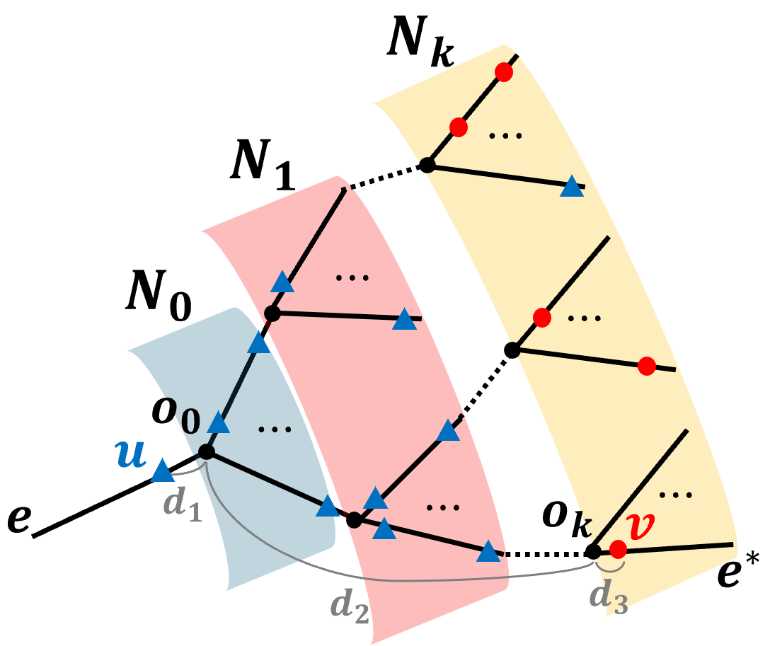
Figure 4: Illustration of the breadth-first search procedure.

According to the above matching process, the distance between a specific $u\in U_{e}^{+}$ and its match $v\in V_{e^{*}}^{+}$ consists of three parts (as indicated by the three gray curves in Figure 4): (i) the distance from $u$ to $o_{0}$ on edge $e$; (ii) the distance from $o_{0}$ to $o_{k}$, where $e^{*}\in N_{k}$; (iii) the distance from $o_{k}$ to $v$ on edge $e^{*}$. Let random variables $d_{1}$, $d_{2}$ and $d_{3}$ represent these three distances, and $\mathbb{E}[X_{\text{G}}^{\text{g}}]$ can be written as the sum of their individual expectations; i.e.,

$$\mathbb{E}[X_{\text{G}}^{\text{g}}] =\mathbb{E}[d_{1}]+\mathbb{E}[d_{2}]+\mathbb{E}[d_{3}].$$ (34)

First, we look at $d_{2}$. The probability of finding a match in the $k$-th layer should be no larger than the probability for at least one edge $e^{\prime}\in N_{k}$ to have $n_{e^{\prime}}>m_{e^{\prime}}$. Since all edges are translationally symmetric, $\text{Pr}\{n_{e^{\prime}}>m_{e^{\prime}}\}=\text{Pr}\{n_{e}>m_{e}\}$. Also, since each node has an equal degree $D$, we have $|N_{k}|\leq(D-1)^{k+1},\operatorname{\forall}k$. Hence, approximately, the probability of finding a match in the $k$-th layer is:

$$1-(1-\text{Pr}\{n_{e}>m_{e}\})^{(D-1)^{k+1}},\quad k=0,1,\cdots.$$ (35)

We would have $d_{2}=kL$ (for $k=0,1,2,\cdots$) if a match is successfully found in the $k$-th layer, but not in the previous layers (if any); hence, for $k=0,1,2,\cdots$:

$$\text{Pr}\{d_{2}=kL\}\approx(1-\text{Pr}\{n_{e}>m_{e}\})^{\sum_{i=0}^{k-1}(D-1)^{i+1}}\cdot[1-(1-\text{Pr}\{n_{e}>m_{e}\})^{(D-1)^{k+1}}].$$ (36)

As $k$ increases, the first term in Equation (36) quickly approaches zero, while the second term approaches a constant. Thus, $\mathbb{E}[d_{2}]$ can be approximated by the following truncation:

$$\mathbb{E}[d_{2}]\approx\sum_{k=0}^{\kappa}kL\cdot\text{Pr}\{d_{2}=kL\},$$ (37)

where $\kappa$ is a relative small value (e.g., about 10).

Next, we look at $d_{1}$ and $d_{3}$. Recall that all unmatched points in $U_{e}^{+}$, if any, after local matching, will be located near the two ends of edge $e$. The expected number of unmatched points near each end is $\frac{\mathbb{E}[|U_{e}^{+}|]}{2}=\frac{1}{2}\mathbb{E}[m_{e}-n_{e}\mid m_{e}>n_{e}]$. The average distance between two adjacent points among them is $\frac{1}{\mu}$. Then, the distance between an arbitrary point $u\in U_{e}^{+}$ and its nearer end $o_{0}$, i.e., $d_{1}$, is approximately uniformly distributed in the interval $\left(0,\frac{1}{2\mu}\mathbb{E}[m_{e}-n_{e}\mid m_{e}>n_{e}]\right)$, and hence the average, $\mathbb{E}[d_{1}]$, is approximately equal to half of the interval length, i.e.,

$$\mathbb{E}[d_{1}]\approx\frac{1}{4\mu}\cdot\mathbb{E}[m_{e}-n_{e}\mid m_{e}>n_{e}],$$ (38)

where $\mathbb{E}[m_{e}-n_{e}\mid m_{e}>n_{e}]$ is given by Equation (31). The derivation of $\mathbb{E}[d_{3}]$ is similar, but through symmetrical analysis of the unmatched points in $V_{e^{*}}^{+}$ where $e^{*}\in N_{k}$. The distance between $o_{k}$ and an arbitrary unmatched point in $V_{e^{*}}^{+}$ near $o_{k}$ is approximately uniformly distributed in the interval $\left(0,\frac{1}{2\lambda}\mathbb{E}[n_{e^{*}}-m_{e^{*}}\mid n_{e^{*}}>m_{e^{*}}]\right)$, and again, $\mathbb{E}[n_{e^{*}}-m_{e^{*}}\mid n_{e^{*}}>m_{e^{*}}]=\mathbb{E}[n_{e}-m_{e}\mid n_{e}>m_{e}]$. However, competition may occur, and not all points in $V_{e^{*}}^{+}$ must be matched. From the perspective of a specific point $u\in U_{e}^{+}$, during the breadth-first search process, it will be matched with the nearest available point $v\in\bigcup_{e^{\prime}\in N_{k}}V_{e^{\prime}}^{+}$. However, other competing points in $\bigcup_{e\in\mathcal{E}}U_{e}^{+}$ (as indicated by the other blue triangles in Figure 4) may also have the chance to be matched with the points in $\bigcup_{e^{\prime}\in N_{k}}V_{e^{\prime}}^{+}$ (shown as the red circles in Figure 4). The expected ratio between the total number of competing points of $u$ and the total number of available points in $\bigcup_{e^{\prime}\in N_{k}}V_{e^{\prime}}^{+}$ is approximately $\frac{|U|}{|V|}=\frac{\mu}{\lambda}$. This indicates that at the end of the breadth-first search process, $\frac{\mu}{\lambda}$ of the points in $\bigcup_{e^{\prime}\in N_{k}}V_{e^{\prime}}^{+}$ will be matched. Since $e^{*}\in N_{k}$, the distance between $o_{k}$ and an arbitrary matched point $v\in V_{e^{*}}^{+}$ near $o_{k}$, i.e., $d_{3}$, is approximately uniformly distributed in the interval $\left(0,\frac{\mu}{2\lambda^{2}}\mathbb{E}[n_{e}-m_{e}\mid n_{e}>m_{e}]\right)$, and hence the average, $\mathbb{E}[d_{3}]$, can be approximately estimated as follows:

$$\mathbb{E}[d_{3}]\approx\frac{\mu}{4\lambda^{2}}\cdot\mathbb{E}[n_{e}-m_{e}\mid n_{e}>m_{e}],$$ (39)

where $\mathbb{E}[n_{e}-m_{e}\mid n_{e}>m_{e}]$ is given by Equation (33).

Summarizing all the above, $\mathbb{E}[X_{\text{G}}]$ can be estimated out of Equations (27)-(39).

4 Numerical Experiment

4.1 Verification of 1D RBNP

In this section, we validate the accuracy of the proposed formulas of 1D RBMP using a series of Monte-Carlo simulations. For each combination of $n$ and $m$ values, 100 RBMP realizations are randomly generated. For each realized instance, the optimal matching is solved by a standard linear program solver GLPK (Makhorin,, 2011). The average optimal matching distances for each $(m,n)$ combination is recorded as the sample mean across the 100 realizations.

Figure 5 compares the simulation results with the formulas developed for both balanced and unbalanced cases, including Equations (6), (21) (22), and (20). The optimal matching distances solved for each instance from the Monte-Carlo simulation is represented by the light-blue dots and their sample mean is represented by the red solid curve with square markers. The estimations from Equations (6), (21), (22), and (20) are marked by the blue dash-dot curves, blue dash-dot curves with cross markers, green dash-dot curves with plus markers, and grey dash curves, respectively.

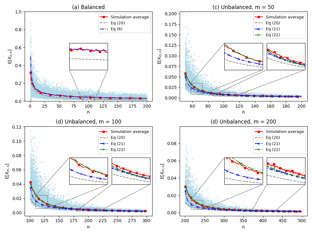
Figure 5: Accuracy of distance estimators.

We first try the balanced cases. Let the value of $n=m$ vary from 1 to 200. Figure 5 (a) shows the results. It can be seen that the estimations by Equation (6) closely match with the simulation averages, with an average relative error of 4.57%. Meanwhile, Equation (20) has a larger average relative error of 43.2%. This indicates that Equation (6) performs significantly better than Equation (20). In addition, when $n$ and $m$ are considerably small, Equation (6) tends to overestimate the simulation average. However, this error diminishes rapidly as $n$ increases. For instance, the relative error is 57.8% when $n=1$, but drops significantly to 9.2% when $n=6$. This deviation is likely due to the assumption of i.i.d. step sizes, as the correlation among the step sizes $l_{i}$ generally decreases with increasing $n$. When $n$ is sufficiently large (e.g., $n>m+100$), Equation (6) can provide a very accurate estimation.

Next, we try the unbalanced cases. We set $m\in\{50,100,200\}$, and let $n$ range from $m+1$ to a sufficiently large number $2m+100$. Figures 5 (b)-(d) show the results. It can be first observed that the estimations from Equation (22) closely match with the simulation averages across all $n$ and $m$ values. The average relative errors are 7.0%, 6.4%, and 5.8% for $m=50,100,200$, respectively. This indicates that, in general, Equation (22) can provide very accurate distance predictions. We then look at the estimations from Equations (21) and (20). It is clear that, when $n\gg m$, both equations also match quite well with the simulation averages. Specifically, for $n\geq 2m$, the average relative errors for Equation (21) are 5.4%, 5.6%, and 6.2%, for $m=50,100,200$, respectively. In the meantime, Equation (20) yields average relative errors of 12.1%, 15.2%, and 17.7% for the same $m$ values, respectively. When $n\approx m$, larger discrepancies can be observed between the equations and the simulation averages. While Equation (21) still outperforms Equation (20), the discrepancy is notable. Recall from Section 2.4.2, this discrepancy may arise from the i.i.d assumption for point selections in $V^{*}$. Observations from various $V^{*}$ instances show that, when $n\approx m$, points at certain specific positions (e.g., the first or the last point when $n=m+1$) are more likely to be selected in $V^{*}$ than the others. Nevertheless, Equation (21) performs generally better than Equation (20) and provides very good estimates when $n\geq 2m$.

In summary, one can choose the most suitable formula given the specific problem setup and the required accuracy. For balanced cases, Equation (6) should be used. For unbalanced cases, when $n\gg m$, Equation (21) is recommended as it can already provide a good estimation and is computationally more efficient than Equation (22); otherwise, Equation (22) is more suitable as it provides the most accurate estimates.

4.2 Verification of Discrete Network RBMP

In this section, we validate the accuracy of the proposed formulas of arbitrary-length line RBMP and discrete network RBMP using a series of Monte-Carlo simulations. For the former, we first fix $\mu$ but vary $L$ and $\lambda$. For the latter, we fix $L$ and $\mu$, but vary $D$ and $\lambda$. For any parameter combination, 100 RBMP instances are randomly generated, each solved through Equation (1)-(2) by a standard linear program solver, and the optimal matching distances are averaged across the 100 realizations.

Figure 6 compares the simulated average distances of arbitrary-length line RBMP, represented by markers, with estimations from Equations (23) (for $\lambda/\mu=1$) and (26) (for $\lambda/\mu\in\{1.1,1.5,3\}$), represented by lines. The line length $L$ varies from $\{1,3,5,7,9\}$ [du], and $\mu=10$ [1/du]. It can be observed that, in general, the estimations by Equations (23) and (26) fit tightly to the simulation averages across all $L$ and $\lambda/\mu$ ratios. The average relative errors by estimations are 5.07%, 6.21%, 2.97%, and 8.84% for $\lambda/\mu=1,1.1,1.5,3$, respectively. Also, it is clear that the optimal matching distance increases concavely with $L$ when $\lambda/\mu=1$. Yet, as the ratio $\lambda/\mu$ becomes slightly larger, both the simulated averages and the formula estimations become flatter. At higher values of $\lambda/\mu$, such as $1.5$ or $3$, there is no significant change in the optimal matching distance with $L$. These observations support the discussion in Section 3.1, and visually illustrates how the average optimal matching distance scales with $\sqrt{L}$ in the balanced RBMP, but is largely independent of $L$ in the unbalanced RBMP with $\lambda\gg\mu$.

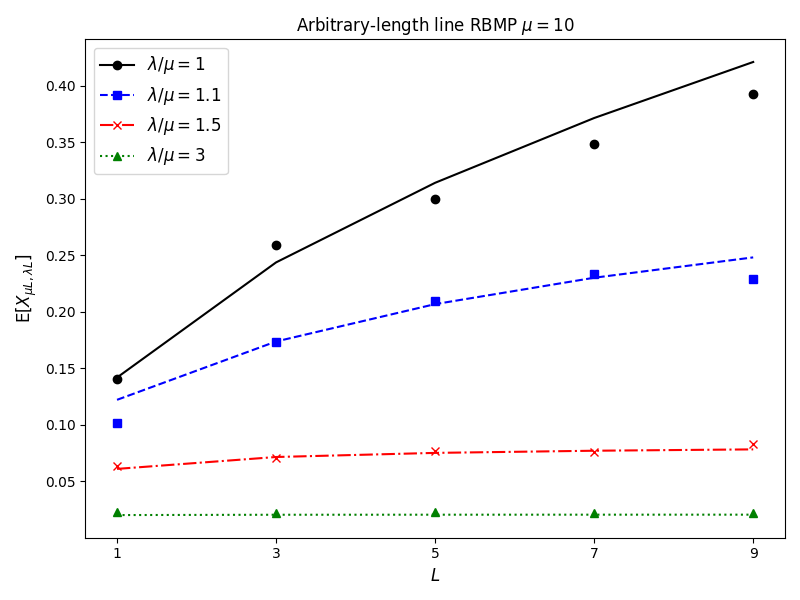
Figure 6: Verification of arbitrary-length 1D RBMP.

Next, we build a series of $D$-regular discrete networks with node degree $D\in\{3,4,6\}$. Each network has 36 total number of unit-length edges (i.e., $L=1$ [du]), and $\mu=5$ [1/du]. We further vary $\lambda$ from 5 to 25 [1/du]. Figures (a)-(c) compare the simulation averages (black solid curve) with estimations by Equation (26) and (27) (dashed and dotted curves). Each Monte-Carlo simulation instance, represented by a light-blue dot, is also plotted. It is observed that the estimations by Equation (27) fit tightly to the simulation average across all parameter combinations. The average relative errors are 8.53%, 4.73%, and 3.40% for $D=3,4,6$, respectively. This indicates that, in general, Equation (27) can provide very accurate predictions in a wide range of $D,L,\lambda/\mu$ combinations. In the meantime, we observe that Equation (26) also estimates the average distance accurately when $\lambda\gg\mu$. Specifically, when $\lambda\geq 2\mu$, the average relative errors of Equation (26) are 9.31%, 6.72%, and 5.96% for $D=3,4,6$, respectively. Recall from Section 3.2, as $\lambda\gg\mu$, there are more chances for a point in $U$ to be matched locally, which indicates that $\alpha$ converges to 0 and Equation (26) will predict the distance almost as as well as Equation (27).

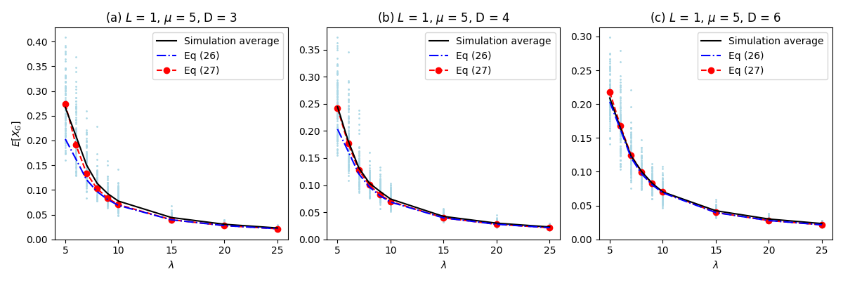
Figure 7: Verification of discrete network RBMP

5 Conclusion

This paper presents a set of closed-form formulas, without curve-fitting or statistical parameter estimation, that can provide accurate estimates for random bipartite matching problems in one-dimensional spaces and discrete networks. These formulas can be directly used in mathematical programs to evaluate and plan resources for many transportation services. In one-dimensional space, we relate the matching distance to the area between a random walk path and the x-axis, and then derive a closed-form formula for balanced matching. For unbalanced matching, we first develop a closed-form but approximate formula by analyzing the properties of unbalanced random walks following the optimal removal of a subset of unmatched points. Then, we introduce a set of recursive formulas that yields tight upper bounds based on the analysis of unbalanced random walks. The scaling property of the matching distance in arbitrary-length line segments is also discussed. Building upon these results, we derive the expected optimal matching distance in a regular-graph, in which points are distributed on equal-length edges based on spatial Poisson processes, by quantifying the expected distance when the point is locally matched (i.e., matched within the same edge) or globally matched (i.e., matched across different edges). Results indicate that our proposed formulas all provide quite accurate distance estimations for one-dimensional line segments and discrete networks under different conditions.

Nevertheless, our proposed models build upon several assumptions and approximations, which may be relaxed in the future. For example, we assumed each random walk step size as an i.i.d random variable with mean $l$, and treat the the mean step size in each balanced random walk segment as the same as that of the original unbalanced random walk. This approach directly leads to an overestimation of the matching distance, particularly when $n\gg m$. Although we propose an approximate correction term in Section 2.4.4 to address this issue, alternative (better) models could be explored in the future. Further analysis could also be conducted to understand how such correlations among matched pairs would affect the optimal point removals for unbalanced problems. In addition, while Section 2.4.3 shows that the distance estimator upper bound is quite accurate, it requires solving a recursive formula, which is computationally more cumbersome. It would be interesting to explore alternative methods that can provide simpler estimates of similar accuracy. For discrete networks, this paper opens the door to many interesting new questions. For example, future research should develop methods to estimate the expected matching distance in networks with varying edge lengths, varying degrees, and heterogeneous point densities.

Appendix. List of notation

Notation	Description
$m,n$	Cardinalities of the two point sets in an one-dimensional RBMP
$U$, $V$	Two sets of points for each one-dimensional RBMP realization
$I$	Set containing all points in $U$ and $V$
$E$	Set of edges connecting $u\in U$ and $v\in V$
$y_{uv}$	1 if $u\in U$ is matched to $v\in V$, 0 otherwise
$X_{m,n}$	Average optimal matching distance per point in an one-dimensional RBMP
$x_{i}$	x-coordinate of a point $i\in I$
$z_{i}$	Supply value of a point $i\in I$
$l_{i}$	Distance (step size) from a point $i\in I$ to its next point
$l$	Mean step size between any two consecutive points in $I$
$S(x;I^{\prime})$	Net supply curve for any coordinate $x$ and subset of points $I^{\prime}\subseteq I$
$A(x;I^{\prime})$	Total absolute area between curve $S(x;I^{\prime})$ and x-axis from 0 to $x$
$Y_{n}$	Total absolute area between any balanced supply curve and x-axis from 0 to 1
$B(n)$	Expected total absolute area between the path of a random walk with $2n$ unit-length steps and x-axis
$V^{\prime}$	An arbitrary set of unmatched/removed points in $V$
$V^{*}$	Optimal set of removed points
$\hat{V}$	Set of removed points from the proposed point removal process
$v^{\prime}_{k},v^{*}_{k},\hat{v}_{k}$	$k$-th removed point along the x-axis in $V^{\prime}$, $V^{*}$, $\hat{V}$
$m_{k}$	Number of demand points in the $k$-th segment of the post-removal curve $S(x;I\setminus V^{*})$
$\hat{m}_{k}$	Number of demand points in the $k$-th segment of the post-removal curve $S(x;I\setminus\hat{V})$
$\hat{m}_{k,0}$	Number of demand points with zero net supplies in the $k$-th segment of the post-removal curve $S(x;I\setminus\hat{V})$
$\hat{Z}_{k,a}$	Total absolute area enclosed by $S(x;I\setminus\hat{V})$ within $(x_{\hat{v}_{k}},1]$, which contains exactly $a$ demand points
$Z_{m,n}$	Total absolute area enclosed by $S(x;I\setminus V^{*})$ from 0 to 1
$L$	Length of a line (edge)
$X_{\text{E}}$	Average optimal matching distance per point on an arbitrary-length line
$\mu,\lambda$	Densities of the two point sets on an arbitrary-length line
$\text{G}=(\mathcal{V},\mathcal{E})$	Graph with node set $\mathcal{V}$ and edge set $\mathcal{E}$
$D$	Degree of node in $\mathcal{V}$
$U_{e},V_{e}$	Realized point sets on an edge $e\in\mathcal{E}$
$m_{e},n_{e}$	Cardinality of point sets $U_{e}$ and $V_{e}$

Notation	Description
$X_{\text{G}}$	Average optimal matching distance per point in a graph
$X^{\text{l}}_{\text{G}},X^{\text{g}}_{\text{G}}$	Average optimal local and global matching distances in a graph
$\alpha$	Probability for global matching
$\phi(\cdot),\Phi(\cdot)$	Probability density function and cumulative distribution function of standard normal distribution
$U_{e}^{+},V_{e}^{+}$	Remaining point sets on an edge $e\in\mathcal{E}$ after local matching process
$N_{k}$	$k$-th layer of edges for a point $u\in U_{e}^{+}$ in breadth-first search
$e^{*}$	Edge containing the matched point $v$ for a point $u\in U_{e}^{+}$
$o_{0}$	Nearer end of $e$ to $u\in U_{e}^{+}$
$o_{k}$	Nearer end of $e^{*}$ to $o_{0}$
$d_{1}$	Distance from $u\in U_{e}^{+}$ to $o_{0}$
$d_{2}$	Distance from $o_{0}$ to $o_{k}$
$d_{3}$	Distance from $o_{k}$ to the matched point $v$ of $u\in U_{e}^{+}$

References

- Abeywickrama et al., (2022) Abeywickrama, T., Liang, V., and Tan, K.-L. (2022). Bipartite matching: What to do in the real world when computing assignment costs dominates finding the optimal assignment. SIGMOD Rec., 51(1):51–58.
- Addario-Berry and Reed, (2008) Addario-Berry, L. and Reed, B. A. (2008). Ballot Theorems, Old and New, pages 9–35. Springer Berlin Heidelberg, Berlin, Heidelberg.
- Afèche et al., (2022) Afèche, P., Caldentey, R., and Gupta, V. (2022). On the optimal design of a bipartite matching queueing system. Operations Research, 70(1):363–401.
- Aloqaily et al., (2022) Aloqaily, M., Bouachir, O., Al Ridhawi, I., and Tzes, A. (2022). An adaptive uav positioning model for sustainable smart transportation. Sustainable Cities and Society, 78:103617.
- Asratian et al., (1998) Asratian, A. S., Denley, T. M. J., and Häggkvist, R. (1998). Bipartite Graphs and their Applications. Cambridge Tracts in Mathematics. Cambridge University Press.
- Caracciolo et al., (2017) Caracciolo, S., D’Achille, M., and Sicuro, G. (2017). Random euclidean matching problems in one dimension. Physical Review E, 96(4).
- Caracciolo et al., (2014) Caracciolo, S., Lucibello, C., Parisi, G., and Sicuro, G. (2014). Scaling hypothesis for the euclidean bipartite matching problem. Physical Review E, 90(1).
- Daganzo, (1978) Daganzo, C. F. (1978). An approximate analytic model of many-to-many demand responsive transportation systems. Transportation Research, 12(5):325–333.
- Daganzo and Smilowitz, (2004) Daganzo, C. F. and Smilowitz, K. R. (2004). Bounds and approximations for the transportation problem of linear programming and other scalable network problems. Transportation Science, 38(3):343–356.
- Ding et al., (2021) Ding, Y., McCormick, S. T., and Nagarajan, M. (2021). A fluid model for one-sided bipartite matching queues with match-dependent rewards. Operations Research, 69(4):1256–1281.
- Dutta and Dasgupta, (2017) Dutta, A. and Dasgupta, P. (2017). Bipartite graph matching-based coordination mechanism for multi-robot path planning under communication constraints. In 2017 IEEE International Conference on Robotics and Automation (ICRA), pages 857–862.
- Ezaki et al., (2024) Ezaki, T., Fujitsuka, K., Imura, N., and Nishinari, K. (2024). Drone-based vertical delivery system for high-rise buildings: Multiple drones vs. a single elevator. Communications in Transportation Research, 4:100130.
- Fedtke and Boysen, (2017) Fedtke, S. and Boysen, N. (2017). A comparison of different container sorting systems in modern rail-rail transshipment yards. Transportation Research Part C: Emerging Technologies, 82:63–87.
- Georgiev and Liò, (2020) Georgiev, D. and Liò, P. (2020). Neural bipartite matching.
- Ghassemi and Chowdhury, (2018) Ghassemi, P. and Chowdhury, S. (2018). Decentralized Task Allocation in Multi-Robot Systems via Bipartite Graph Matching Augmented With Fuzzy Clustering. volume Volume 2A: 44th Design Automation Conference of International Design Engineering Technical Conferences and Computers and Information in Engineering Conference, page V02AT03A014.
- Harel, (1993) Harel, A. (1993). Random walk and the area below its path. Mathematics of Operations Research, 18(3):566–577.
- Hernández et al., (2021) Hernández, D., Cecília, J. M., Calafate, C. T., Cano, J.-C., and Manzoni, P. (2021). The kuhn-munkres algorithm for efficient vertical takeoff of uav swarms. In 2021 IEEE 93rd Vehicular Technology Conference (VTC2021-Spring), pages 1–5.
- Jin et al., (2022) Jin, C., Xu, J., Han, Y., Hu, J., Chen, Y., and Huang, J. (2022). Efficient delay-aware task scheduling for iot devices in mobile cloud computing. Mobile Information Systems, 2022(1):1849877.
- Jonker and Volgenant, (1987) Jonker, R. and Volgenant, A. (1987). A shortest augmenting path algorithm for dense and sparse linear assignment problems. Computing, 38(4):325–340.
- Kuhn, (1955) Kuhn, H. W. (1955). The hungarian method for the assignment problem. Naval Research Logistics Quarterly, 2:83–97.
- Makhorin, (2011) Makhorin, A. (2011). GLPK (GNU Linear Programming Kit) v4.65. Department for Applied Informatics, Moscow Aviation Institute, Moscow. https://www.gnu.org/software/glpk/glpk.html.
- Mezard and Parisi, (1985) Mezard, M. and Parisi, G. (1985). Replicas and optimization. http://dx.doi.org/10.1051/jphyslet:019850046017077100, 46.
- Mézard and Parisi, (1988) Mézard, M. and Parisi, G. (1988). The Euclidean matching problem. Journal de Physique, 49(12):2019–2025.
- Ouyang and Yang, (2023) Ouyang, Y. and Yang, H. (2023). Measurement and mitigation of the “wild goose chase” phenomenon in taxi services. Transportation Research Part B: Methodological, 167:217–234.
- Panigrahy et al., (2020) Panigrahy, N. K., Basu, P., Nain, P., Towsley, D., Swami, A., Chan, K. S., and Leung, K. K. (2020). Resource allocation in one-dimensional distributed service networks with applications. Performance Evaluation, 142:102110.
- Seth et al., (2023) Seth, A., James, A., Kuantama, E., Mukhopadhyay, S., and Han, R. (2023). Drone high-rise aerial delivery with vertical grid screening. Drones, 7(5).
- Shen and Ouyang, (2023) Shen, S. and Ouyang, Y. (2023). Dynamic and pareto-improving swapping of vehicles to enhance integrated and modular mobility services. Transportation Research Part C: Emerging Technologies, 157:104366.
- Shen et al., (2024) Shen, S., Zhai, Y., and Ouyang, Y. (2024). Expected bipartite matching distance in a -dimensional space: Approximate closed-form formulas and applications to mobility services. https://arxiv.org/abs/2406.12174.
- Stiglic et al., (2015) Stiglic, M., Agatz, N., Savelsbergh, M., and Gradisar, M. (2015). The benefits of meeting points in ride-sharing systems. Transportation Research Part B: Methodological, 82:36–53.
- Tafreshian and Masoud, (2020) Tafreshian, A. and Masoud, N. (2020). Trip-based graph partitioning in dynamic ridesharing. Transportation Research Part C: Emerging Technologies, 114:532–553.
- Wang et al., (2016) Wang, X., He, F., Yang, H., and Oliver Gao, H. (2016). Pricing strategies for a taxi-hailing platform. Transportation Research Part E: Logistics and Transportation Review, 93:212–231.
- Wang et al., (2004) Wang, Y., Makedon, F., Ford, J., and Huang, H. (2004). A bipartite graph matching framework for finding correspondences between structural elements in two proteins. In The 26th Annual International Conference of the IEEE Engineering in Medicine and Biology Society, volume 2, pages 2972–2975.
- Yang et al., (2010) Yang, H., Leung, C., Wong, S., and Bell, M. (2010). Equilibria of bilateral taxi–customer searching and meeting on networks. Transportation Research Part B: Methodological, 44:1067–1083.
- Zhang et al., (2014) Zhang, Y., Phillips, C. A., Rogers, G. L., Baker, E. J., Chesler, E. J., and Langston, M. A. (2014). On finding bicliques in bipartite graphs: a novel algorithm and its application to the integration of diverse biological data types. BMC Bioinformatics, 15(1):110.
- Zhou et al., (2022) Zhou, Y., Yang, H., and Ke, J. (2022). Price of competition and fragmentation in ride-sourcing markets. Transportation Research Part C: Emerging Technologies, 143:103851.