Primal-dual Accelerated Mirror-Descent Method for Constrained Bilinear Saddle-Point Problems

Abstract

We develop a first-order accelerated algorithm for a class of constrained bilinear saddle-point problems with applications to network systems. The algorithm is a modified time-varying primal-dual version of an accelerated mirror-descent dynamics. It deals with constraints such as simplices and convex set constraints effectively, and converges with a rate of $\mathcal{O}(1/t^{2})$. Furthermore, we employ the acceleration scheme to constrained distributed optimization and bilinear zero-sum games, and obtain two variants of distributed accelerated algorithms.

I INTRODUCTION

Constrained bilinear saddle-point problems (BSPPs) aim at seeking saddle points that minimize global functions in one direction and maximize them in the other, where decision variables are limited to certain feasible regions or ranges. BSPPs arise from convex optimization with affine constraints via Lagrangian methods [1], while constraints are significant in applications including multi-robot motion planning, resource allocation in communication networks, and economic dispatch in power grids. Constrained BSPPs appear in various scenarios such as robust optimization, signal processing, and machine learning [2], and thus, a substantial effort has been paid to design effective algorithms to solve them. Particularly, first-order methods are frequently used since they only involve gradient information and are suitable for large-scale problems. First-order primal-dual methods have been widely investigated. They are powerful for constrained optimization/game problems, and easy to be implemented both in centralized and distributed manners [3, 4, 5].

Motivated by big-data advances and privacy concerns encountered in practice, the areas of distributed optimization and games over multi-agent systems have received much attention, with applications to unmanned systems, smart grids, and social networks [6, 7]. Some of the formulations could be cast into constrained BSPPs, and then, solved by primal-dual methods [7, 8, 9, 10]. For instance, a discrete-time primal-dual algorithm was designed for a constrained distributed optimization problem in [9], while a continuous-time version was proposed for a distributed extended monotropic optimization problem in [8]. In [10], a distributed primal-dual algorithm with a fixed stepsize was developed to handle coupled constraints. Additionally, a primal-dual framework was explored for two-network zero-sum games in [7]. However, existing results indicate that standard primal-dual methods could only achieve asymptotic convergence with a rate of $\mathcal{O}(1/t)$ for general convex cost functions [8, 9].

Various accelerated protocols have been explored for convex optimization, for example the well-known heavy-ball algorithm [11]. The author of [12] showed that first-order methods have an optimal rate of $\mathcal{O}(1/t^{2})$ in the worst case. Then the Nesterov’s accelerated scheme was proposed in [12], and a continuous-time version was developed in [13]. In [14], an accelerated method was explored under regularity conditions. In [15], a class of zero-order optimization dynamics was proposed with acceleration and restarting mechanisms. However, these results are mainly devoted to unconstrained optimization. For consensus-based distributed optimization, a fast gradient algorithm, with a rate of $\mathcal{O}(1/t^{1.4-\epsilon})$, was designed in [16], while a Nesterov’s accelerated algorithm, with a rate of $\mathcal{O}(1/t^{2-\epsilon})$, was developed in [17]. However, both of them were primal-based and only handled consensus type constraints. In order to solve convex optimization with affine constraints or BSPPs, attempts have been made by combining accelerated protocols with primal-dual methods. For instance, an accelerated primal-dual method, using adaptive parameters, was designed with a rate of $\mathcal{O}(1/t^{2})$ in [18]. In [2], an accelerated gradient method, with an optimal linear rate, was developed. In [19], lower bounds of the gradient computation burden were provided, and then, a corresponding algorithm was proposed with complexity guarantees. However, the algorithms in [18, 2, 19] require strong convexity on cost functions, which does not hold in applications such as data analysis and machine learning [20]. In [21], by incorporating the Nesterov’s acceleration into a primal-dual framework, a continuous-time accelerated dynamics was designed for strictly convex cost functions. Afterwards, the protocol was adopted to seek Nash equlibria for two-network bilinear zero-sum games in [22]. It has been shown that the algorithms in [21, 22] achieved a rate of $\mathcal{O}(1/t^{2})$, but neither of them can handle optimization/game problems beyond affine constraints, including set constraints. To the best of our knowledge, few accelerated primal-dual algorithms, dealing with strictly convex cost functions and set constraints at the same time, achieve a rate of $\mathcal{O}(1/t^{2})$.

The mirror-descent algorithm, proposed in [23], is a generalization of gradient-based methods by introducing a Bregman distance function in place of the Euclidean distance. It can solve constrained optimization problems [24], and has generated a lot of interest. For instance, linear rates of mirror-descent and actor-critic dynamics were analyzed in [25, 26]. In [27], a second-order mirror-descent dynamics was proposed for merely monotone games. In [28], a primal-dual version was designed for distributed optimization. In [29], an accelerated mirror-descent scheme, regarded as an extension of the Nesterov’s acceleration, was developed with a rate of $\mathcal{O}(1/t^{2})$. However, existing literature has not provided any accelerated mirror-descent algorithm under a primal-dual framework.

In this paper, we focus on developing such a continuous-time algorithm. On the one hand, continuous-time algorithms have received a flurry of research interest with applications in multi-agent systems. For cyber-physical systems with physical systems acting or moving in real time, they are quite natural, and meanwhile, can be implemented by hardware devices such as analog circuits [30]. The continuous-time design has been reported in existing literature, including [3, 4, 10, 7, 31, 15]. On the other hand, continuous-time algorithms can serve as a tool for understanding, analyzing and generalizing the discrete-time algorithms [32, 33, 13]. Our main contributions are summarized as follows.

1. We propose a time-varying primal-dual mirror-descent algorithm to solve a constrained BSPP, which covers many problems including convex optimization with affine constraints [21, 18], constrained distributed optimization [9], and bilinear games [22]. The algorithm is a modified primal-dual version of the dynamics in [29], has a unique solution, and can efficiently handle set constraints, simplices, etc.

2. We establish that the algorithm converges with a rate of $\mathcal{O}(1/t^{2})$ (in terms of the duality gap function), which is faster than the primal-dual methods in [3, 4, 5].

3. Resorting to the accelerated protocol, we provide two variants of distributed algorithms for constrained distributed optimization and for bilinear zero-sum games. We show that they have faster rates than those of [8, 9, 31, 7].

This paper is organized as follows. Some preliminaries are introduced in Section II. Section III formulates the problem, and presents the accelerated algorithm. Our main results are provided in Section IV, and two distributed algorithms are obtained for network optimization and games in Section V. Finally, concluding remarks are given in Section VI.

II Preliminary Background

Let $\mathbb{R}$, $\mathbb{N}$, $\mathbb{R}^{p}$ and $\mathbb{R}^{p\times q}$ be the set of real numbers, nonnegative integers, $p$-dimensional real column vectors and $p$-by-$q$ real matrices. Denote $0_{p}$ as the $p$-dimensional zero vector, and $I_{p}$ as the $p$-by-$p$ identity matrix. Denote $(\cdot)^{\rm T}$, $\otimes$ and $\|\!\cdot\!\|$ as the transpose, the Kronecker product, and the Euclidean norm. For $x,y\in\mathbb{R}^{p}$, their Euclidean inner product is $x^{\rm T}y$ or $\langle x,y\rangle$. Let $X\times Y$ be the Cartesian product of sets $X$ and $Y$. For a differentiable function $S(x,y)$, $\nabla_{x}S(x,y)$ is the partial gradient of $S$ with respect to $x$. Let $\{x_{n}(t)\}_{n\in\mathbb{N}}$ be a family of functions from $\mathbb{R}$ to $\mathbb{R}^{p}$. The sequence is equi-continuous if for any $\epsilon>0$, there always exists $\delta>0$ such that $\|x_{n}(t+h)-x_{n}(t)\|<\epsilon,\forall|h|<\delta,\forall n\in\mathbb{N}$.

Let $\Omega\subset\mathbb{R}^{p}$ be a closed convex set. The normal cone of $\Omega$ at $x\in\Omega$ is $\mathcal{N}_{\Omega}(x)=\{v\in\mathbb{R}^{p}|v^{\rm T}(y-x)\leq 0,\forall y\in\Omega\}.$ Take $P_{\Omega}(u)={\rm argmin}_{v\in\Omega}\|v-u\|$. Then $\langle v-P_{\Omega}(u),u-P_{\Omega}(u)\rangle\leq 0,~{}\forall u\in\mathbb{R}^{p},~{}\forall v\in\Omega$.

Take $\mathbb{E}=\mathbb{R}^{p}$. Given an extended real-valued function $\psi:\mathbb{E}\rightarrow[-\infty,+\infty]$, it is proper if it does not attain the value $-\infty$, and there exists at least one $x\in\mathbb{E}$ such that $\psi(x)<\infty$. Besides, it is closed if its epigraph is closed. The domain of $\psi$ is ${\rm dom}(\psi)=\{x\in\mathbb{E}:\psi(x)<\infty\}$. The function $\psi^{*}:\mathbb{E}^{*}\rightarrow[-\infty,+\infty]$, defined by $\psi^{*}(z)=\sup_{x\in\mathbb{E}}\{x^{T}z-\psi(x)\}$, is called the conjugate function of $\psi$, where $\mathbb{E}^{*}$ is the dual space of $\mathbb{E}$. If $\psi$ is proper, then $\psi^{*}$ is closed and convex. The Bregman divergence of a proper, closed and convex function $\psi$ is $D_{\psi}(x,y)=\psi(x)-\psi(y)-\langle x-y,\nabla\psi(y)\rangle$. Referring to [34], we have the following result.

Lemma 1

Let $\psi:\mathbb{R}^{p}\rightarrow\mathbb{R}\cup\{\infty\}$ be a closed, proper and strongly convex function, where $\Omega:={\rm dom}(\psi)$ is a closed convex set. Then $\psi^{*}$ is differentiable and convex such that

$$\nabla{\psi}^{*}(z)={\rm argmin}_{x\in\Omega}\{-x^{\rm T}z+\psi(x)\}.$$ (1)

Consider a multi-agent network described by an undirected graph $\mathcal{G}(\mathcal{V},\mathcal{E})$, where $\mathcal{V}=\{1,\dots,n\}$ is the node set and $\mathcal{E}\subset\mathcal{V}\times\mathcal{V}$ is the edge set. The graph $\mathcal{G}$ is associated with an adjacency matrix $\mathcal{A}=[a_{ij}]\in\mathbb{R}^{n\times n}$ such that $a_{ij}=a_{ji}>0$ if $(i,j)\in\mathcal{E}$, and $a_{ij}=0$ otherwise. The Laplacian matrix $\mathcal{L}$ is $\mathcal{L}=\mathcal{D}-\mathcal{A}$, where $\mathcal{D}={\rm diag}\{d_{i}\}\in\mathbb{R}^{n\times n}$, and $d_{i}=\sum_{j\in\mathcal{V}}a_{ij}$. Graph $\mathcal{G}$ is connected if there exists a path between any pair of distinct nodes.

III PROBLEM SETUP AND ALGORITHM

In this section, we give the problem statement and propose an accelerated algorithm.

III-A Problem Formulation

Consider a constrained BSPP given by

$$\min_{x\in X}~{}\max_{y\in Y}~{}L(x,y):=F(x)+x^{\rm T}Hy-G(y)$$ (2)

where $X\subset\mathbb{R}^{p}$ and $Y\subset\mathbb{R}^{q}$ are closed constraint sets, $H\in\mathbb{R}^{p\times q}$ is a known matrix, and moreover, $F:X\rightarrow\mathbb{R}$ and $G:Y\rightarrow\mathbb{R}$ are continuous functions. A profile $(x^{\star},y^{\star})\in X\times Y$ is called a saddle point (or a solution) to (2) if

$$L(x^{\star},y)\leq L(x^{\star},y^{\star})\leq L(x,y^{\star}),~{}~{}\forall x\in X,~{}\forall y\in Y.$$

We make the following well-known assumption for (2).

Assumption 1

The sets $X$ and $Y$ are nonempty, closed and convex. The functions $F$ and $G$ are continuously differentiable and strictly convex on two open sets containing $X$ and $Y$. The gradients of $F$ and $G$ are Lipschitz continuous over $X$ and $Y$. Moreover, there exists a unique saddle point to (2).

Remark 1

Problem (2) is a general model, and appears in constrained optimization, bilinear games and multi-agent systems [1, 9, 7]. It generalizes the models in [21, 22] by allowing the constraints $X$ and $Y$, and covers the problems in [2, 18, 19] since $F$ and $G$ are only required to be strictly convex rather than strongly convex.

First-order primal-dual methods in [3, 4, 5] can be employed to solve (2). However, they suffer from a slow convergence rate. Existing works indicate that mirror-descent methods, powerful for constrained optimization, can achieve acceleration [23, 24, 29]. The observations motivate us to design a novel accelerated algorithm by incorporating an accelerated mirror-descent protocol into a primal-dual framework.

III-B Accelerated Algorithm Design

Consider $X=\mathbb{R}^{p}$ and $Y=\mathbb{R}^{q}$. Referring to [3, 4, 5], a first-order primal-dual dynamics for (2) is given by

$$\dot{x}= -\nabla_{x}L(x,y)=-\nabla F(x)-Hy$$ (3)

$$\dot{y}= ~{}~{}~{}\nabla_{y}L(x,y)=-\nabla G(y)+H^{\rm T}x$$

where $x(0)=x_{0}\in\mathbb{R}^{p}$, $y(0)=y_{0}\in\mathbb{R}^{q}$, and $\dot{x}={\rm d}x(t)/{\rm d}t$ is the derivative of $x$ with respect to time $t$. We omit time $t$ in remaining of this paper without causing confusions. Clearly, the variable $x$ descents in the direction of negative gradient of $L$, while $y$ ascents in the other direction.

Given a closed convex set $\Omega\subset\mathbb{R}^{p}$ and a continuously differential and convex function $f:\Omega\rightarrow\mathbb{R}$, an accelerated mirror-descent algorithm is designed in [29] as

$$\dot{x}=\frac{r}{t}\big{[}\nabla\psi^{*}(z)-x\big{]},~{}\dot{z}=-\frac{t}{r}\nabla f(x)$$ (4)

where $r>0$, $\psi$ is a generating function with ${\rm dom}(\psi)=\Omega$, $\psi^{*}$ is the convex conjugate of $\psi$, $z(0)=z_{0}$ and $x(0)=x_{0}=\nabla\psi^{*}(z_{0})$. If $\nabla\psi^{*}(z)=z$, then (4) recovers the continuous-time Nesterov’s accelerated algorithm in [13]. By [29, Th. 2], (4) converges with a rate of $\mathcal{O}(1/t^{2})$ if $r\geq 2$.

Inspired by (3) and (4), we propose a continuous-time primal-dual accelerated algorithm as

$$\dot{x}= \frac{r}{t}\big{[}\nabla\psi^{*}(u)-x\big{]},~{}\dot{y}=\frac{r}{t}\big{[}\nabla\phi^{*}(v)-y\big{]}$$ (5)

$$\dot{u}= \frac{t}{r}\big{[}\!-\nabla F(x)-H(y+\frac{t}{r}\dot{y})+\nabla\psi(x+\frac{t}{r}\dot{x})-u\big{]}$$

$$\dot{v}= \frac{t}{r}\big{[}\!-\nabla G(y)+H^{\rm T}(x+\frac{t}{r}\dot{x})+\nabla\phi(y+\frac{t}{r}\dot{y})-v\big{]}$$

where $\psi:\mathbb{R}^{p}\rightarrow\mathbb{R}\cup\{\infty\}$ and $\phi:\mathbb{R}^{q}\rightarrow\mathbb{R}\cup\{\infty\}$ are proper, closed and convex functions with ${\rm dom}(\psi)=X$ and ${\rm dom}(\phi)=Y$, $x(0)=x_{0}=\nabla\psi^{*}(u_{0})$, $u(0)=u_{0}=\nabla\psi(x_{0})$, $y(0)=y_{0}=\nabla\phi^{*}(v_{0})$, and $v(0)=v_{0}=\nabla\phi(y_{0})$.

The following assumption is needed for $\psi$ and $\phi$ [29, 26].

Assumption 2

Both $\psi:\mathbb{R}^{p}\rightarrow\mathbb{R}\cup\{\infty\}$ and $\phi:\mathbb{R}^{q}\rightarrow\mathbb{R}\cup\{\infty\}$ are proper, closed, and strongly convex functions, where ${\rm dom}(\psi)$ and ${\rm dom}(\phi)$ are nonempty, closed and convex sets, which equal to $X$ and $Y$, respectively. They are also continuously differentiable with Lipschitz continuous gradients on their domains. Besides, $\nabla\psi^{*}$ and $\nabla\phi^{*}$ are Lipschitz continuous over $X$ and $Y$.

Remark 2

The initial states, including $x_{0}=\nabla\psi^{*}(u_{0})$, $y_{0}=\nabla\phi^{*}(v_{0})$, $u_{0}=\nabla\psi(x_{0})$ and $v_{0}=\nabla\phi(y_{0})$, ensure (5) has a unique solution as will be shown in Theorem 1, and they are satisfied by taking $u_{0}\in X$ and $v_{0}\in Y$. In order to guarantee $(x^{\star},y^{\star})$ is a solution to (2) at the equilibrium point $(u^{\star},x^{\star},v^{\star},y^{\star})$ of (5) as will be proved in Lemma 3, the extra terms $\nabla\psi(x+\frac{t}{r}\dot{x})-u$ and $\nabla\phi(y+\frac{t}{r}\dot{y})-v$ are designed in the evolution of $u$ and $v$. Additionally, inspired by [35], we introduce the derivative feedbacks $\dot{x}$ and $\dot{y}$, as damping terms, for the convergence of (5).

Remark 3

In fact, (5) is a generalization of (4) in [29] under a primal-dual framework. Compared with the second-order mirror-descent dynamics in [27], (5) is only a first-order algorithm, and hence, $F$ and $G$ are assumed to be strictly convex for its exact convergence. We focus on a sublinear rate instead of linear convergence, and thus, we do not impose that $F$ and $G$ are strongly convex as [26] did. While the discounted mirror-descent dynamics only achieved perturbed Nash equilibriums for monotone games [25, 26], (5) reaches the exact saddle point of (2) as will be proved in Theorem 2. Furthermore, it has a faster rate than the algorithm in [28]. If the constraints $X$ and $Y$ in (2) disappear, (5) degenerates into the primal-dual Nesterov’s accelerated algorithms in [21, 22] by taking $\nabla\psi^{*}(u)=u$ and $\nabla\phi^{*}(v)=v$.

The introduction of $\psi$ and $\phi$ makes it possible to analyze and design mirror-descent algorithms from the dual space of the Euclidean space. In practice, they can be employed to deal with some constraints efficiently. We provide the following two examples for illustration, and recommend readers to refer to [26, 27] for more details.

1. Let $X$ be a nonempty, closed and convex set. Consider $\psi(x)=\frac{1}{2}\|x\|^{2},x\in X$. Then $\nabla\psi^{*}(u)=P_{X}(u)$.

2. Let $X$ be a simplex, i.e., $X=\{x=[x_{i}]\in\mathbb{R}^{p}~{}|~{}x_{i}\geq 0,\sum_{i}x_{i}=1\}$. Take $\phi(x)=\sum_{i}x_{i}\log(x_{i}),x\in X$, where $0{\rm log}(0)=0$. Then $\nabla\psi^{*}(u)=\big{[}\frac{\exp(u_{i})}{\sum_{i}\exp(u_{i})}\big{]}$.

IV MAIN RESULTS

This section analyzes properties of (5), including the existence of a solution, the optimality and the convergence.

For convenience, we define $z=[x^{\rm T},y^{\rm T}]^{\rm T},w=[u^{\rm T},v^{\rm T}]^{\rm T}$, $\nabla R(z)=[\nabla F^{\rm T}(x),\nabla G^{\rm T}(y)]^{\rm T}$, $\tilde{H}=[0_{p\times p},H;-H^{\rm T},0_{q\times q}]$, $\nabla\pi^{*}(w)=[\nabla\psi^{*{\rm T}}(u),\nabla\phi^{*{\rm T}}(v)]^{\rm T}$, and $\nabla\pi(z)=[\nabla\psi^{\rm T}(x),\nabla\phi^{\rm T}(y)]^{\rm T}$. Then dynamics (5) reads as

$$\dot{z}= \frac{r}{t}\big{[}\nabla\pi^{*}(w)-z\big{]}$$ (6)

$$\dot{w}= \frac{t}{r}\big{[}\!-\nabla R(z)-\tilde{H}(z+\frac{t}{r}\dot{z})+\nabla\pi(z+\frac{t}{r}\dot{z})-w\big{]}$$

where $z(0)=z_{0}=\nabla\pi^{*}(w_{0})$, and $w(0)=w_{0}=\nabla\pi(z_{0})$.

Classical results in ordinary differential equations (ODEs) do not directly imply the existence and uniqueness of a solution to (6) since $r/t$ is singular at $t=0$. For the analysis, we define an approximate smooth dynamics as

$$\dot{z}= \frac{r}{\max(\delta,t)}\big{[}\nabla\pi^{*}(w)-z\big{]}$$ (7)

$$\dot{w}= \frac{t}{r}\big{[}\!-\nabla R(z)-\tilde{H}(z+\frac{t}{r}\dot{z})+\nabla\pi(z+\frac{t}{r}\dot{z})-w\big{]}$$

where $\delta>0$, $z(0)=z_{0}=\nabla\pi^{*}(w_{0})$, and $w(0)=w_{0}=\nabla\pi(z_{0})$. Under Assumptions 1 and 2, (7) has a unique solution $\big{(}z_{\delta}(t),w_{\delta}(t)\big{)}$ by [36, Th. 3.2]. In addition, we have the following result, whose proof is given in the Appendix.

Lemma 2

Consider dynamics (7). If Assumptions 1 and 2 hold, then there exists a small enough $t_{m}$ such that the family of solutions $\big{(}(z_{\delta}(t),w_{\delta}(t))|_{[0,t_{m}]}\big{)}_{\delta\leq t_{m}}$ is equi-continuous and uniformly bounded.

First, we establish that there is a unique solution to (6).

Theorem 1

If Assumptions 1 and 2 hold, then dynamics (6) has a unique solution $(z(t),w(t))$ for all $t\geq 0$.

Proof: Here we show that there exists a solution to (6). Uniqueness of the solution is proved in the Appendix.

Let $\delta_{i}=2^{-i}t_{m}$ for $i\in\mathbb{N}$, and $(z_{\delta_{i}},w_{\delta_{i}})$ be a family of solutions to (7) defined on $[0,t_{m})$. By Lemma 2, the family is equi-continuous and uniformly bounded. Resorting to the Arzela-Ascoli theorem [37, Th. 10.1], there must be a subsequence $(z_{\delta_{i}},w_{\delta_{i}})_{i\in\mathcal{I}}$ that converges uniformly to a limit $(\bar{z},\bar{w})$, where $\mathcal{I}\subset\mathbb{N}$ is an infinite set of indices.

We now prove that $(\bar{z},\bar{w})$ is a solution to (6). Clearly, the initial conditions hold. Take $t_{3}\in[0,t_{m})$, and let $(\tilde{z},\tilde{w})$ be a solution to (6) on $t\geq t_{3}$ with initial condition $\big{(}\bar{z}(t_{3}),\bar{w}(t_{3})\big{)}$. Since $\lim_{i\to\infty}\big{(}z_{\delta_{i}}(t_{3}),w_{\delta_{i}}(t_{3})\big{)}_{i\in\mathcal{I}}=\big{(}\bar{z}(t_{3}),\bar{w}(t_{3})\big{)}$, it follows from [38, Th. 2.8] that $(z_{\delta_{i}},w_{\delta_{i}})$ converges to $(\tilde{z},\tilde{w})$ uniformly on $[t_{3},t_{3}+\epsilon)$ for some $\epsilon>0$. Note that $(z_{\delta_{i}},w_{\delta_{i}})_{i\in\mathcal{I}}$ also converges to $(\bar{z},\bar{w})$. Thus, $(\bar{z},\bar{w})$ coincides with $(\tilde{z},\tilde{w})$ on $[t_{3},t_{3}+\epsilon)$, and $(\bar{z},\bar{w})$ is a solution to (6) on $[t_{3},t_{3}+\epsilon]$. Due to the arbitrariness of $t_{3}$, (6) has a solution. $\hfill\square$

The next lemma addresses the relationship between the saddle point of (2) and an equilibrium point of (5).

Lemma 3

Under Assumptions 1 and 2, $(x^{\star},y^{\star})$ is the solution to (2) if and only if there exists $(u^{\star},v^{\star})$ such that $(x^{\star},u^{\star},y^{\star},v^{\star})$ is an equilibrium point of dynamics (5).

Proof: If $(x^{\star},u^{\star},y^{\star},v^{\star})$ is an equilibrium point of (5), then

$$0_{p}= ~{}\nabla\psi^{*}(u^{\star})-x^{\star},~{}0_{q}=\nabla\phi^{*}(v^{\star})-y^{\star}$$

$$0_{p}= -\nabla F(x^{\star})-Hy^{\star}+\nabla\psi(x^{\star})-u^{\star}$$

$$0_{q}= -\nabla G(y^{\star})+H^{\rm T}x^{\star}+\nabla\psi(y^{\star})-v^{\star}.$$

Recalling (1) gives $u^{\star}-\nabla\psi(x^{\star})\in\mathcal{N}_{X}(x^{\star})$ and $v^{\star}-\nabla\psi(y^{\star})\in\mathcal{N}_{Y}(y^{\star})$. Therefore, $-\nabla F(x^{\star})-Hy^{\star}\in\mathcal{N}_{X}(x^{\star})$, and $-\nabla G(y^{\star})+H^{\rm T}x^{\star}\in\mathcal{N}_{Y}(y^{\star})$. It follows from the Karush–Kuhn–Tucker (KKT) optimality conditions [1, Th. 3.34] that $(x^{\star},y^{\star})$ is the saddle point of $L$.

Conversely, suppose that $(\tilde{x},\tilde{y})$ is the saddle point of $L$. Take $\tilde{u}-\nabla\psi(\tilde{x})=-\nabla F(\tilde{x})-H\tilde{y}\in\mathcal{N}_{X}(\tilde{x})$, and $\tilde{v}-\nabla\phi(\tilde{y})=-\nabla G(\tilde{y})+H^{\rm T}\tilde{x}\in\mathcal{N}_{Y}(\tilde{y})$. Then $\tilde{x}=\nabla\psi^{*}(\tilde{u})$, and $\tilde{y}=\nabla\phi^{*}(\tilde{v})$. Thus, $(\tilde{x},\tilde{u},\tilde{y},\tilde{v})$ is the equilibrium point of (5), and the proof is completed. $\hfill\square$

Before proving the convergence of (5), we provide a supporting lemma as follows.

Lemma 4

Consider dynamics (5). Under Assumptions 1 and 2, $x(t)\in X$, and $y(t)\in Y$ for all $t\geq 0$.

Proof: Define $h(t)=\frac{1}{2}\|x-P_{X}(x)\|^{2}$. Clearly,

$$\dot{h}(t)=\langle x-P_{X}(x),\dot{x}\rangle=\frac{r}{t}\langle x-P_{X}(x),\nabla\psi^{*}(u)-x\rangle$$

$$=-\frac{r}{t}\|x-P_{X}(u)\|^{2}+\frac{r}{t}\langle x-P_{X}(x),\nabla\psi^{*}(u)-P_{X}(x)\rangle.$$

By (1), $\nabla\psi^{*}(u)\in X$, and then, $\langle x-P_{X}(x),\nabla\psi^{*}(u)-P_{X}(x)\rangle\leq 0$. It follows that $\dot{h}(t)\leq 0$. Since $x_{0}\in X$, $h(t)=0$, i.e., $x(t)\in X,~{}\forall t\geq 0$. Similarly, $y(t)\in Y,~{}\forall t\geq 0$. This completes the proof. $\hfill\square$

Finally, we analyze the convergence of (5).

Theorem 2

Suppose Assumptions 1 and 2 hold. Let $\big{(}x(t),\\ u(t),y(t),v(t)\big{)}$ be a trajectory of (5), and $(x^{\star},u^{\star},y^{\star},v^{\star})$ be an equilibrium point of (5), where $r\geq 2$, and $(x^{\star},y^{\star})$ is the saddle point of (2).

1. The duality gap, defined by $L(x(t),y^{\star})-L(x^{\star},y(t))$, converges to $0$ with a rate of $\mathcal{O}(1/t^{2})$.

2. The trajectory of $\big{(}x(t),y(t)\big{)}$ approaches $(x^{\star},y^{\star})$.

Proof: By Lemma 3, $(x^{\star},y^{\star})$ is the saddle point of (2) for any equilibrium point $(x^{\star},u^{\star},y^{\star},v^{\star})$ of (5). Define

$$V=\frac{t^{2}}{r}\big{(}L(x,y^{\star})-L(x^{\star},y)\big{)}+rD_{\psi^{*}}(u,u^{\star})+rD_{\phi^{\star}}(v,v^{\star})$$ (8)

where $D_{\psi^{*}}$ and $D_{\phi^{*}}$ are the Bregman divergence of $\psi^{*}$ and $\phi^{*}$. Recalling Lemma 4 gives $L(x,y^{\star})-L(x^{\star},y)\geq 0$, where the equality holds only if $x=x^{\star}$ and $y=y^{\star}$. Due to the convexity of $\psi^{*}$ and $\phi^{*}$, $D_{\psi^{*}}(u,u^{\star})+D_{\phi^{\star}}(v,v^{\star})\geq 0$. Hence, $V\geq 0$, and moreover, $V=0$ only if $(x,y)=(x^{\star},y^{\star})$.

Combining (5) with (8), we obtain

$$\dot{V} =\frac{2t}{r}\big{(}L(x,y^{\star})-L(x^{\star},y)\big{)}+t\langle\nabla F(x)+Hy^{\star},$$

$$~{}~{}~{}\nabla\psi^{*}(u)-x\rangle+t\langle\nabla G(y)-H^{\rm T}x^{\star},\nabla\phi^{*}(v)-y\rangle$$

$$+r\langle\nabla\psi^{*}(u)-\nabla\psi^{*}(u^{\star}),\dot{u}\rangle+r\langle\nabla\phi^{*}(v)-\nabla\phi^{*}(v^{\star}),\dot{v}\rangle.$$

Note that

$$t\langle\nabla F(x)+Hy^{\star},\nabla\psi^{*}(u)-x\rangle+r\langle\nabla\psi^{*}(u)-\nabla\psi^{*}(u^{\star}),\dot{u}\rangle$$

$$=t\langle x+\frac{t}{r}\dot{x}-x^{\star},-H(y+\frac{t}{r}\dot{y}-y^{\star})+\nabla\psi(x+\frac{t}{r}\dot{x})-u\rangle$$

$$-t\langle x-x^{\star},\nabla F(x)+Hy^{\star}\rangle$$

and moreover,

$$t\langle\nabla G(y)-H^{\rm T}x^{\star},\nabla\phi^{*}(v)-y\rangle+r\langle\nabla\phi^{*}(v)\!-\!\nabla\phi^{*}(v^{\star}),\dot{v}\rangle$$

$$=t\langle y+\frac{t}{r}\dot{y}-y^{\star},H^{\rm T}(x+\frac{t}{r}\dot{x}-x^{\star})+\nabla\phi(y+\frac{t}{r}\dot{y})-v\rangle$$

$$-t\langle y-y^{\star},\nabla G(y)-H^{\rm T}x^{\star}\rangle.$$

Consequently,

$$\dot{V} =\frac{2t}{r}\big{(}L(x,y^{\star})-L(x^{\star},y)\big{)}$$ (9)

$$-t\langle x-x^{\star},\nabla F(x)+Hy^{\star}\rangle-t\langle y-y^{\star},\nabla G(y)-H^{\rm T}x^{\star}\rangle$$

$$+t\langle\nabla\psi^{*}(u)-x^{\star},\nabla\psi(x+\frac{t}{r}\dot{x})-u\rangle$$

$$+t\langle\nabla\phi^{*}(v)-y^{\star},\nabla\phi(y+\frac{t}{r}\dot{y})-v\rangle.$$

Since $x+\frac{t}{r}\dot{x}=\nabla\psi^{*}(u)$, $\nabla\psi(x+\frac{t}{r}\dot{x})-u\in-\mathcal{N}_{X}(x+\frac{t}{r}\dot{x})$ by Lemma 1. Therefore,

$$\langle \nabla\psi^{*}(u)-x^{\star},\nabla\psi(x+\frac{t}{r}\dot{x})-u\rangle$$

$$=\langle x+\frac{t}{r}\dot{x}-x^{\star},\nabla\psi(x+\frac{t}{r}\dot{x})-u\rangle\leq 0.$$

Similarly, $\langle\nabla\phi^{*}(v)-y^{\star},\nabla\phi(y+\frac{t}{r}\dot{y})-v\rangle\leq 0.$ Due to the convexity of $F$ and $G$, we obtain

$$L(x^{\star},y)-L(x,y^{\star})\geq\langle x^{\star}-x,\nabla F(x)+Hy^{\star}\rangle$$

$$+\langle y^{\star}-y,\nabla G(y)-H^{\rm T}x^{\star}\rangle$$ .

By (9), $\dot{V}\leq(\frac{2t}{r}-t)\big{(}L(x,y^{\star})-L(x^{\star},y)\big{)}$. As a result, $\dot{V}\leq 0$ if $r\geq 2$. Let $m_{0}=V(x_{0},u_{0},y_{0},v_{0})$. Then $V\leq m_{0},\forall t\geq 0$. Furthermore, $L(x,y^{\star})-L(x^{\star},y)\leq\frac{r}{t^{2}}V\leq\frac{r}{t^{2}}m_{0}$, i.e., $L(x,y^{\star})-L(x^{\star},y)$ converges to $0$ with a rate of $\mathcal{O}(1/t^{2})$. Therefore, part (i) is proved.

It is clear that $L(x,y^{\star})-L(x^{\star},y^{\star})\leq L(x,y^{\star})-L(x^{\star},y)\leq\frac{r}{t^{2}}m_{0}$. Since $F$ is strictly convex, $L(x,y^{\star})$ has a unique minimizer, and as a result, $x(t)$ converges to $x^{\star}$. By a similar procedure, $y(t)$ approaches $y^{\star}$. Thus, part (ii) is proved, and the proof is completed. $\hfill\square$

Theorem 2 indicates that (5) reaches the exact saddle point of (2) with a rate of $\mathcal{O}(1/t^{2})$. It has a faster performance than the primal-dual methods in [8, 9, 7, 31]. Besides, as a first-order algorithm, (5) has an optimal rate in the worst case [12, Th. 2.1.7].

Remark 4

In fact, the order of the convergence rate of (5) remains unchanged if its right-hand side is multiplied by a positive constant gain. However, time-varying gains should be carefully chosen because they may produce unbounded variable derivatives and make algorithms impractical.

Remark 5

The continuous-time algorithm (5) may be discretized for its numerical implementation. Referring to [39], there are various discretization schemes for an ODE. By numerical tests, we have observed that using a similar discretization scheme as that of [29], the corresponding discrete-time algorithm from (5) still maintains the acceleration characteristics. The convergence, robustness and numerical stability of the scheme will be investigated in the future.

V DISTRIBUTED APPLICATIONS

In this section, we apply the proposed algorithm (5) to constrained distributed optimization and two-network bilinear zero-sum games.

V-A Constrained Distributed Optimization

Consider a network of $n$ agents interacting over an undirected and connected graph $\mathcal{G}(\mathcal{V},\mathcal{E})$, where agent $i$ only knows a local function $f_{i}:\Omega_{i}\rightarrow\mathbb{R}$ and a closed set $\Omega_{i}\subset\mathbb{R}^{p}$, and all agents cooperate to find a consensus solution that minimizes the global function $\sum_{i\in\mathcal{V}}f_{i}(x)$. The problem is formulated as

$$\min~{}f(\bm{x}):=\sum\nolimits_{i\in\mathcal{V}}f_{i}(x_{i})~{}~{}{\rm s.t.}~{}\bm{L}\bm{x}=0,~{}\bm{x}\in\Omega$$ (10)

where $\bm{x}=[x_{1}^{\rm T},\dots,x_{n}^{\rm T}]^{\rm T}\in\mathbb{R}^{pn}$, $\mathcal{L}\in\mathbb{R}^{n\times n}$ is the Laplacian matrix of $\mathcal{G}$, $\bm{L}=\mathcal{L}\otimes I_{p}\in\mathbb{R}^{pn\times pn}$ and $\Omega=\Omega_{1}\times\dots\times\Omega_{n}$.

We make the following assumption for (10).

Assumption 3

For $i\in\mathcal{V}$, $\Omega_{i}$ is closed and convex, $f_{i}$ is continuously differentiable and strictly convex on an open set containing $\Omega_{i}$, and $\nabla f_{i}$ is Lipschitz continuous over $\Omega_{i}$. The Slater’s condition holds, and there exists a unique solution.

To solve (10), distributed algorithms have been explored in [9, 6] with applications in motion planning, alignment of multiple vehicles and distributed optimal consensus of multi-agent systems. Due to the presence of $\Omega$, the accelerated protocol in [21] cannot be adopted.

Referring to [9], we first reformulate (10) as

$$\min_{\bm{x}\in\Omega}~{}\max_{\bm{y}\in\mathbb{R}^{pn}}~{}S_{1}(\bm{x},\bm{y}):=f(\bm{x})+\bm{y}^{\rm T}\bm{L}\bm{x}+\frac{1}{2}\bm{x}^{\rm T}\bm{L}\bm{x}$$ (11)

where $\bm{y}=[y_{1}^{\rm T},\dots,y_{n}^{\rm T}]^{\rm T}\in\mathbb{R}^{pn}$ is the dual variable. Then we introduce variables $\bm{u}=[u_{1}^{\rm T},\dots,u_{n}^{\rm T}]^{\rm T}\in\mathbb{R}^{pn}$ and $\bm{v}=[v_{1}^{\rm T},\dots,v_{n}^{\rm T}]^{\rm T}\in\mathbb{R}^{pn}$, and generating functions $\psi_{i}$ with $\nabla\psi_{i}^{*}(u_{i})=P_{\Omega_{i}}(u_{i})$. Following that, the accelerated distributed algorithm is given by

$$\dot{x}_{i}= \frac{r}{t}\big{[}P_{\Omega_{i}}(u_{i})-x_{i}\big{]},~{}\dot{y}_{i}=\frac{r}{t}\big{[}v_{i}-y_{i}\big{]}$$ (12)

$$\dot{u}_{i}= \frac{t}{r}\big{[}\!-\nabla_{x_{i}}S_{1}(\bm{x},\bm{y}+\frac{t}{r}\dot{\bm{y}})+x_{i}+\frac{t}{r}\dot{x}_{i}-u_{i}\big{]}$$

$$\dot{v}_{i}= \frac{t}{r}\big{[}\nabla_{y_{i}}S_{1}(\bm{x}+\frac{t}{r}\dot{\bm{x}},\bm{y})+y_{i}+\frac{t}{r}\dot{y}_{i}-v_{i}\big{]}$$

where $x_{i}(0)=x_{i,0}=u_{i,0}$, $u_{i}(0)=u_{i,0}\in\Omega_{i}$, $y_{i}(0)=y_{i,0}=v_{i,0}$, and $v_{i}(0)=v_{i,0}\in\mathbb{R}^{p}$.

Finally, we establish the convergence of (12) as follows.

Corollary 1

Suppose Assumption 3 holds. Let $\big{(}\bm{x}(t),\bm{u}(t),\\ \bm{y}(t),\bm{v}(t)\big{)}$ be a trajectory of (12), and $(\bm{x}^{\star},\bm{u}^{\star},\bm{y}^{\star},\bm{v}^{\star})$ be an equilibrium point of (12), where $r\geq 2$, $(\bm{x}^{\star},\bm{y}^{\star})$ is a saddle point of $S_{1}$, and $\bm{x}^{\star}$ is the optimal solution to (10).

1. The duality gap, defined by $S_{1}\big{(}\bm{x}(t),\bm{y}^{\star}\big{)}-S_{1}\big{(}\bm{x}^{\star},\bm{y}(t)\big{)}$, converges to $0$ with a rate of $\mathcal{O}(1/t^{2})$.

2. The trajectory of $\bm{x}(t)$ approaches $\bm{x}^{\star}$.

3. Both $\|\bm{L}\bm{x}\|$ and $|f(\bm{x})-f(\bm{x}^{\star})|$ converge to $0$ with a rate of $\mathcal{O}(1/t)$.

Proof: By a similar procedure as the proof of Theorem 2, items (i) and (ii) hold resorting to a function defined as

$$V_{1}=\frac{t^{2}}{r}\big{(}S_{1}(\bm{x},\bm{y}^{\star})-S_{1}(\bm{x}^{\star},\bm{y})\big{)}+rD_{\psi^{*}}(\bm{u},\bm{u}^{\star})+rD_{\phi^{*}}(\bm{v},\bm{v}^{\star})$$

where $D_{\psi^{*}}(\bm{u},\bm{u}^{\star})=\sum_{i\in\mathcal{V}}D_{\psi_{i}^{*}}(u_{i},u_{i}^{\star})$, $D_{\phi^{*}}(\bm{v},\bm{v}^{\star})=\sum_{i\in\mathcal{V}}D_{\phi_{i}^{*}}(v_{i},v_{i}^{\star})$, $D_{\psi_{i}^{*}}$ and $D_{\phi_{i}^{*}}$ are the Bregman divergence, $\psi_{i}(x_{i})=\frac{1}{2}\|x_{i}\|^{2},x_{i}\in\Omega_{i}$, and $\phi_{i}(y_{i})=\frac{1}{2}\|y_{i}\|^{2},y_{i}\in\mathbb{R}^{p}$.

Since $S_{1}(\bm{x},\bm{y}^{\star})-S_{1}(\bm{x}^{\star},\bm{y})\geq\frac{1}{2}\bm{x}^{T}\bm{L}\bm{x}$, it follows from (i) that $\|\bm{L}\bm{x}\|$ approaches $0$ with a rate of $\mathcal{O}(1/t)$. In addition, $0\leq f(\bm{x})+\bm{y}^{\star T}\bm{L}\bm{x}-f(\bm{x}^{*})\leq S_{1}(\bm{x},\bm{y}^{*})-S_{1}(\bm{x}^{*},\bm{y})$, and as a result,

$$|f(\bm{x})-f(\bm{x}^{\star})|\leq\|\bm{y}^{\star}\|\cdot\|\bm{L}\bm{x}\|+S_{1}(\bm{x},\bm{y}^{\star})-S_{1}(\bm{x}^{\star},\bm{y}).$$

Therefore, $|f(\bm{x})-f(\bm{x}^{\star})|$ converges to $0$ with a rate of $\mathcal{O}(1/t)$, and item (iii) holds. The proof is completed. $\hfill\square$

Remark 6

We should mention that (10) has a unique solution $\bm{x}^{\star}$, but admits multiple dual variables $\bm{y}^{*}$ such that $(\bm{x}^{\star},\bm{y}^{\star})$ is a saddle point of $S_{1}$ [40]. Thus, we only analyze the converge of $\bm{x}(t)$. Referring to [18, 32], we convert the convergence result on the duality gap into the constraint violation and the primal suboptimality in Corollary 1 (iii).

V-B Two-Network Bilinear Zero-Sum Games

Consider two undirected and connected networks $\mathcal{G}_{1}(\mathcal{V}_{1},\mathcal{E}_{1})$ and $\mathcal{G}_{2}(\mathcal{V}_{2},\mathcal{E}_{2})$ with $n_{1}$ and $n_{2}$ agents, where agent $i$ in $\mathcal{G}_{1}$ knows a function $f_{i}:X_{i}\rightarrow\mathbb{R}$ and a constraint set $X_{i}\subset\mathbb{R}^{p}$, and moreover, agent $j$ in $\mathcal{G}_{2}$ knows a function $g_{j}:Y_{j}\rightarrow\mathbb{R}$ and a constraint set $Y_{j}\subset\mathbb{R}^{q}$. Let $X=X_{1}\times\cdots\times X_{n_{1}}$ and $Y=Y_{1}\times\cdots\times Y_{n_{2}}$. The payoff function $U(\bm{x},\bm{y}):X\times Y\rightarrow\mathbb{R}$ of the zero-sum game is

$$U(\bm{x},\bm{y}):=\tilde{f}(\bm{x})+\bm{x}^{\rm T}B\bm{y}-\tilde{g}(\bm{y})$$

where $\bm{x}=[x_{1}^{\rm T},\dots,x^{\rm T}_{n_{1}}]^{\rm T}$, $\bm{y}=[y^{\rm T}_{1},\dots,y^{\rm T}_{n_{2}}]^{\rm T}$, $\tilde{f}(\bm{x})=\sum_{i\in\mathcal{V}_{1}}f_{i}(x_{i})$, $\tilde{g}(\bm{y})=\sum_{j\in\mathcal{V}_{2}}g_{j}(y_{j})$, $\bm{x}^{\rm T}B\bm{y}=\sum_{i\in\mathcal{V}_{1}}\sum_{j\in\mathcal{V}_{2}}x_{i}^{\rm T}H_{ij}y_{j}$, and $H_{ij}\in\mathbb{R}^{p\times q}$ is a non-zero matrix only if agent $i$ of $\mathcal{G}_{1}$ and agent $j$ of $\mathcal{G}_{2}$ can observe each other’s decision variable. Feasibility sets of $\mathcal{G}_{1}$ and $\mathcal{G}_{2}$ are $\Omega_{1}=\{\bm{x}\in X:x_{1}=\dots=x_{n_{1}}\}$ and $\Omega_{2}=\{\bm{y}\in Y:y_{1}=\dots=y_{n_{2}}\}$. Seeking an Nash equilibrium of the game can be cast into

$$\min_{\bm{x}\in X}\max_{\bm{y}\in Y}~{}U(\bm{x},\bm{y})~{}~{}{\rm s.t.}~{}\bm{L}_{1}\bm{x}=0_{pn_{1}},~{}\bm{L}_{2}\bm{y}=0_{qn_{2}}$$ (13)

where $\mathcal{L}_{1}$ and $\mathcal{L}_{2}$ are the Laplacian matrices of $\mathcal{G}_{1}$ and $\mathcal{G}_{2}$, $\bm{L}_{1}=\mathcal{L}_{1}\otimes I_{p}\in\mathbb{R}^{pn_{1}\times pn_{1}}$, and $\bm{L}_{2}=\mathcal{L}_{2}\otimes I_{q}\in\mathbb{R}^{qn_{2}\times qn_{2}}$.

We make the following assumption for (13).

Assumption 4

For each $i\in\mathcal{V}_{1}$ and $j\in\mathcal{V}_{2}$, $f_{i}$ and $g_{j}$ are continuously differentiable and strictly convex on two open sets containing $X_{i}$ and $Y_{j}$, respectively. Their gradients are Lipschitz continuous over $X_{i}$ and $Y_{j}$. Moreover, the Slater’s condition holds, and there exists a unique Nash equilibrium.

Problem (13) models distributed optimization with parameter uncertainties, and arises in distributed adversarial resource allocation of multiple communication channels [7].

It follows from [22] that (13) can be reformulated as

$$\min_{\bm{x},\bm{\mu}}~{}\max_{\bm{y},\bm{\lambda}}~{}S_{2}(\bm{x},\bm{\lambda},\bm{y},\bm{\mu}):=U(\bm{x},\bm{y})+\bm{\lambda}^{\rm T}\bm{L}_{1}\bm{x}$$ (14)

$$-\bm{\mu}^{\rm T}\bm{L}_{2}\bm{y}+\frac{1}{2}\bm{x}^{\rm T}\bm{L}_{1}\bm{x}-\frac{1}{2}\bm{y}^{\rm T}\bm{L}_{2}\bm{y}$$

where $\bm{\lambda}=[\lambda_{1}^{\rm T},\dots,\lambda_{n_{1}}^{\rm T}]^{\rm T}\in\mathbb{R}^{pn_{1}}$ and $\bm{\mu}=[\mu_{1}^{\rm T},\dots,\mu_{n_{2}}^{\rm T}]^{\rm T}\in\mathbb{R}^{qn_{2}}$ are dual variables for the consensus constraints.

We introduce variables $\bm{u}=[u_{1}^{\rm T},\dots,u_{n_{1}}^{\rm T}]^{\rm T}\in\mathbb{R}^{pn_{1}}$, $\bm{\tau}=[\tau_{1}^{\rm T},\dots,\tau_{n_{1}}^{\rm T}]^{\rm T}\in\mathbb{R}^{pn_{1}}$, $\bm{v}=[v_{1}^{\rm T},\dots,v_{n_{2}}^{\rm T}]^{\rm T}\in\mathbb{R}^{qn_{2}}$, and $\bm{\nu}=[\nu_{1}^{\rm T},\dots,\nu_{n_{2}}^{\rm T}]^{\rm T}\in\mathbb{R}^{qn_{2}}$. Consider the corresponding distributed accelerated algorithm from (5) as

$$\dot{x}_{i}= \frac{r}{t}\big{[}\nabla\psi_{i}^{*}(u_{i})-x_{i}\big{]},~{}\dot{\lambda}_{i}=\frac{r}{t}\big{[}\tau_{i}-\lambda_{i}\big{]}$$ (15)

$$\dot{u}_{i}= \frac{t}{r}\big{[}\!-\!\nabla_{x_{i}}\!S_{2}\big{(}\bm{x},\bm{\lambda}\!+\!\frac{t}{r}\dot{\bm{\lambda}},y\!+\!\frac{t}{r}\dot{\bm{y}},\bm{\mu}\big{)}\!+\!\nabla\psi_{i}\big{(}x_{i}\!+\!\frac{t}{r}\dot{x}_{i}\big{)}\!-\!u_{i}\big{]}$$

$$\dot{\tau}_{i}= \frac{t}{r}\big{[}\nabla_{\lambda_{i}}S_{2}\big{(}\bm{x}+\frac{t}{r}\dot{\bm{x}},\bm{\lambda},\bm{y},\bm{\mu}\big{)}+\lambda_{i}+\frac{t}{r}\dot{\lambda_{i}}-\tau_{i}\big{]}$$

$$\dot{y}_{j}= \frac{r}{t}\big{[}\nabla\phi_{j}^{*}(v_{j})-y_{j}\big{]},~{}\dot{\mu}_{j}=\frac{r}{t}\big{[}\nu_{j}-\mu_{j}\big{]}$$

$$\dot{v}_{j}= \frac{t}{r}\big{[}\nabla_{y_{j}}\!S_{2}\big{(}\bm{x}\!+\!\frac{t}{r}\dot{\bm{x}},\bm{\lambda},\bm{y},\bm{\mu}\!+\!\frac{t}{r}\dot{\bm{\mu}}\big{)}\!+\!\nabla\phi_{j}(y_{j}\!+\!\frac{t}{r}\dot{y}_{j})\!-\!v_{j}\big{]}$$

$$\dot{\nu}_{j}= \frac{t}{r}\big{[}\!-\nabla_{\mu_{i}}S_{2}\big{(}\bm{x},\bm{\lambda},\bm{y}+\frac{t}{r}\dot{\bm{y}},\bm{\mu}\big{)}+\mu_{j}+\frac{t}{r}\dot{\mu_{j}}-\nu_{j}\big{]}$$

where $x_{i}(0)\!=\!x_{i,0}\!=\!\nabla\psi_{i}^{*}(u_{i,0})$, $u_{i}(0)\!=\!u_{i,0}\in X_{i}$, $\lambda_{i}(0)\!=\!\lambda_{i,0}\!=\!\tau_{i,0}$, $\tau_{i}(0)\!=\!\tau_{i,0}\in\mathbb{R}^{p}$, $y_{j}(0)\!=\!y_{j,0}\!=\!\nabla\phi_{i}^{*}(v_{j,0})$, $v_{j}(0)\!=\!v_{j,0}\in Y_{j}$, $\mu_{j}(0)\!=\!\mu_{j,0}\!=\!\nu_{i,0}$ and $\nu_{j}(0)\!=\!\nu_{j,0}\in\mathbb{R}^{q}$. The generating functions $\psi_{i}$ and $\phi_{j}$, depending on $X_{i}$ and $Y_{j}$, are manually selected with similar requirements as that of $\psi$ and $\phi$ in Assumption 2. Clearly, (15) covers the algorithm in [22], but $\psi_{i}$ and $\phi_{i}$ are introduced to handle constraints. Its convergence is addressed as follows.

Corollary 2

Suppose Assumption 4 holds. Let $\big{(}\bm{x}(t),\bm{u}(t),\\ \bm{\lambda}(t),\bm{\tau}(t),\bm{y}(t),\bm{v}(t),\bm{\mu}(t),\bm{\nu}(t)\big{)}$ be a trajectory of (15), and $(\bm{x}^{\star},\bm{u}^{\star},\bm{\lambda}^{\star},\bm{\tau}^{\star},\bm{y}^{\star},\bm{v}^{\star},\bm{\mu}^{\star},\bm{\nu}^{\star})$ be an equilibrium point of (15). where $r\geq 2$, $(\bm{x}^{\star},\bm{\lambda}^{\star},\bm{y}^{\star},\bm{\mu}^{\star})$ is a saddle point of $S_{2}$, and $(\bm{x}^{\star},\bm{y}^{\star})$ is the NE of (13).

1. The duality gap, defined by $S_{2}\big{(}\bm{x}(t),\bm{\lambda}^{\star},\bm{y}^{\star},\bm{\mu}(t)\big{)}-S_{2}(\bm{x}^{\star},\bm{\lambda}(t),\bm{y}(t),\bm{\mu}^{\star})$, converges to $0$ with a rate of $\mathcal{O}(1/t^{2})$.

2. The trajectory of $\big{(}\bm{x}(t),\bm{y}(t)\big{)}$ approaches $(\bm{x}^{\star},\bm{y}^{\star})$.

3. All $\|\bm{L}_{1}\bm{x}\|$, $\|\bm{L}_{2}\bm{y}\|$ and $|U(\bm{x},\bm{y}^{\star})-U(\bm{x}^{\star},\bm{y})|$ converge to $0$ with a rate of $\mathcal{O}(1/t)$.

Proof: The proof of items (i) and (ii) is similar to that of Theorem 2 by defining a function as

$$V_{2}= \frac{t^{2}}{r}\big{(}S_{2}(\bm{x},\bm{\lambda}^{\star},\bm{y}^{\star},\bm{\mu})-S_{2}(\bm{x}^{\star},\bm{\lambda},\bm{y},\bm{\mu}^{\star})\big{)}+rD_{\psi_{u}^{*}}(\bm{u},\bm{u}^{\star})$$

$$+rD_{\psi_{\tau}^{*}}(\bm{\tau},\bm{\tau}^{\star})+rD_{\phi_{v}^{*}}(\bm{v},\bm{v}^{\star})+rD_{\phi_{\nu}^{*}}(\bm{\nu},\bm{\nu}^{\star})$$

where $D_{\psi_{u}^{*}}(\bm{u},\bm{u}^{\star})=\sum_{i\in\mathcal{V}_{1}}D_{\psi_{i}^{*}}(u_{i},u_{i}^{\star})$, $D_{\psi_{\tau}^{*}}(\bm{\tau},\bm{\tau}^{\star})=\sum_{i\in\mathcal{V}_{1}}D_{\widetilde{\psi}_{i}^{*}}(\tau_{i},\tau_{i}^{\star})$ $D_{\phi_{v}^{*}}(\bm{v},\bm{v}^{\star})=\sum_{j\in\mathcal{V}_{2}}D_{\phi_{j}^{*}}(v_{j},v_{j}^{\star})$, $D_{\phi_{\nu}^{*}}(\bm{\nu},\bm{\nu}^{\star})=\sum_{j\in\mathcal{V}_{2}}D_{\widetilde{\phi}_{j}^{*}}(\nu_{j},\nu_{j}^{\star})$, $\widetilde{\psi}_{i}(\lambda_{i})=\frac{1}{2}\|\lambda_{i}\|^{2},\lambda_{i}\in\mathbb{R}^{p}$, and $\widetilde{\phi}_{j}(\mu_{j})=\frac{1}{2}\|\mu_{j}\|^{2},\mu_{j}\in\mathbb{R}^{q}$. The proof of item (iii) can refer to that of Corollary 1 (iii). $\hfill\square$

V-C Numerical Simulations

Here we provide two examples for illustration.

Example 1

Consider problem (10), where $n=20$, each node of $\mathcal{G}$ connects with the others with a probability of $0.7$. For $i\in\mathcal{V}$, $f_{i}$ is a logistic regression function given by $f_{i}(x_{i})=\frac{1}{m_{i}}\sum_{j=1}^{m_{i}}\log\big{[}1+\exp\big{(}\!-(a_{ij}^{T}\hat{x}_{i}+x_{i,0})l_{ij}\big{)}\big{]}$, and $\Omega_{i}=\{x_{i}\in\mathbb{R}^{p}:\|x_{i}\|\leq c\}$, where $x_{i}=[x_{i,0},\hat{x}_{i}^{T}]^{T}\in\mathbb{R}^{p}$, $p=10$, $m_{i}=5$, $c=100$, all entries of $a_{ij}\in\mathbb{R}^{p-1}$ are randomly drawn from $[0,1]$, and $l_{ij}$ is a random number in $\{-1,+1\}$. We solve the problem by the accelerated algorithm (12) and the primal-dual method in [31], where we approximate trajectories of the continuous-time dynamics using function ode45 of Matlab. Fig. 1(a) shows the trajectories of $\log[S_{1}(\bm{x},\bm{y}^{\star})-S_{1}(\bm{x}^{\star},\bm{y})]$, and indicates that (12) has a faster rate than the standard primal-dual algorithm. It is also clear that for (12), the trajectory of the duality gap is not guaranteed to be monotone with respect to time, which is similar to that of Nesterov’s acceleration for unconstrained optimization. Fig. 1(b) implies that all agents reach a consensus solution due to $\lim_{t\to\infty}\|\bm{L}\bm{x}\|=0$.

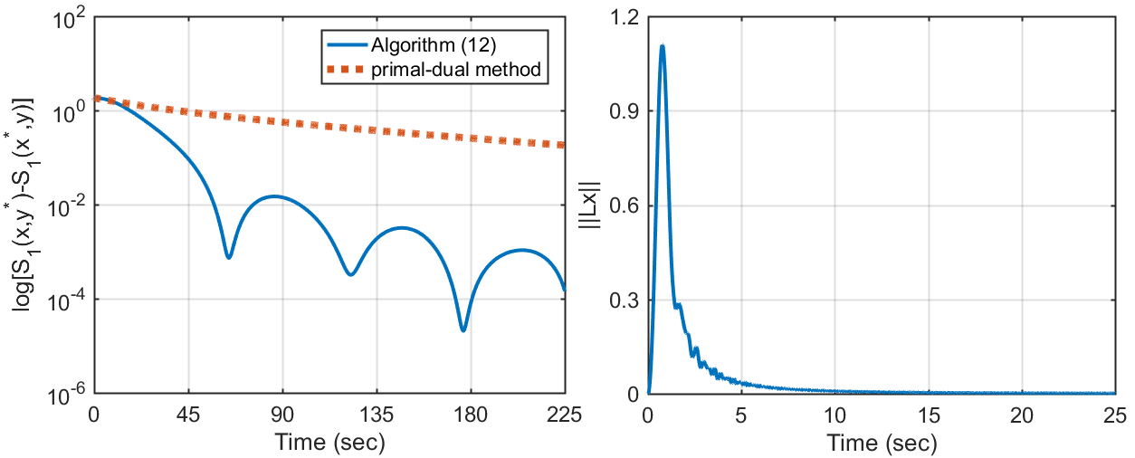
Figure 1: (a) Comparative results for (12) and the primal-dual method in [31]. (b) The trajectory of $\|\bm{L}\bm{x}\|$.

Example 2

Consider problem (13), where $n_{1}=n_{2}=10$, $p=q=20$, $B$ is an identity matrix, each node of $\mathcal{G}_{1}$ connects with the others with a probability of $0.6$, and $\mathcal{G}_{2}$ is generated by a similar procedure as that of $\mathcal{G}_{1}$. Each $f_{i}$ is a linear function as $f_{i}(x_{i})=a_{i}^{\rm T}x_{i}+b_{i}$, $g_{j}$ is a log-sum-exp function as $g_{j}(y_{j})=\rho\log\big{[}\sum_{k=1}^{m}\exp(c_{jk}^{T}y_{j}-d_{jk})/\rho\big{]}$, $X_{i}=\{x_{i}\in\mathbb{R}^{p}~{}|~{}l_{i}\leq x_{i}\leq u_{i}\}$, and $Y_{j}=\mathbb{R}^{q}$, where entries of $a_{i}\in\mathbb{R}^{p}$ and $b_{i}$ are randomly drawn from $[0,1]$, entries of $l_{i}$ and $u_{i}$ are random vectors drawn from $[-2,0]$ and $[1,5]$, $\rho=20$, $m=8$, $c_{jk}\in\mathbb{R}^{q}$ is a random vector from i.i.d standard Guassian distribution, and $d_{jk}\in\mathbb{R}$ is a random number from Guassian distribution with mean $0$ and variance $2$. Fig. 2(a) presents the trajectories of $U(\bm{x},\bm{y})$ under dynamics (15) and the primal-dual method in [7], and indicates that (15) converges with a faster rate. Fig. 2(b) implies that the constraints of (13) are satisfied as $t$ tends to infinity.

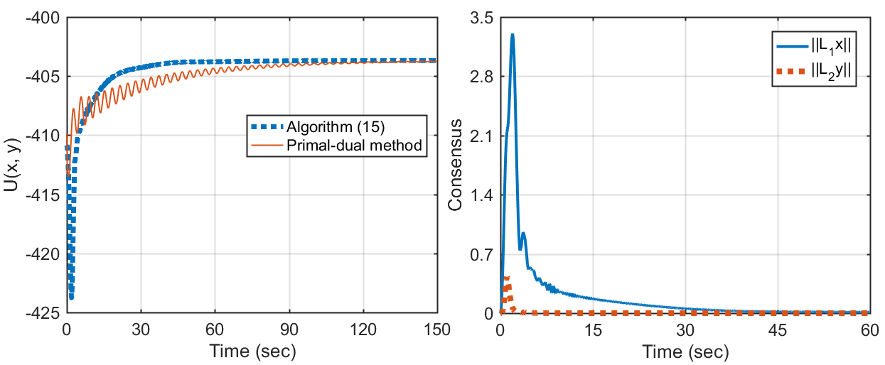
Figure 2: (a) Comparative results for (15) and the primal-dual method in [7]. (b) Trajectories of $\|\bm{L}_{1}\bm{x}\|$ and $\|\bm{L}_{2}\bm{y}\|$.

VI CONCLUSION

This paper considered solving a class of constrained saddle point problems. Inspired by a primal-dual framework, we proposed a novel continuous-time accelerated mirror-descent algorithm. We showed that the algorithm converged with a rate of $\mathcal{O}(1/t^{2})$, which was faster than the standard primal-dual method. Following that, two distributed accelerated algorithms were obtained for constrained distributed optimization and two-network bilinear zero-sum games. Numerical simulations were also provided for verification.

Proof of Lemma 2: Under Assumptions 1 and 2, (7) has a unique solution on $[0,t_{0}]$ for some $t_{0}>0$. Define $A_{\delta}(t)=\sup_{0\leq s\leq t}\|\dot{w}_{\delta}(s)\|/s$, $B_{\delta}(t)=\sup_{0\leq s\leq t}\|z_{\delta}(s)-z_{0}\|/s$, and $C_{\delta}(t)=\sup_{0\leq s\leq t}\|\dot{z}_{\delta}(s)\|$. It is clear that

$$\|\dot{w}_{\delta}(t)\| \leq\frac{t}{r}\|\nabla R(z_{\delta}(t))\|+\frac{t}{r}\lambda_{H}\|z_{\delta}(t)\|+\frac{t^{2}}{r^{2}}\lambda_{H}\|\dot{z}_{\delta}(t)\|$$

$$+\frac{t}{r}\|\nabla\pi(z_{\delta}(t)+\frac{t}{r}\dot{z}_{\delta}(t))-w_{\delta}(t)\|$$

where $\lambda_{H}$ is the maximal singular value of $\tilde{H}$.

Let $L_{\pi}$, $L_{\pi^{*}}$ and $L_{R}$ be the Lipschitz constants of $\nabla\pi$, $\nabla\pi^{*}$ and $\nabla R$ over $X\times Y$. We first show that $z_{\delta}(t)+\frac{t}{r}\dot{z}_{\delta}(t)\in X\times Y$ for all $t\geq 0$. If $t\geq\delta$, $z_{\delta}(t)+\frac{t}{r}\dot{z}_{\delta}(t)=\nabla\pi^{*}(w_{\delta}(t))\in X\times Y$ by Lemma 1. If $t<\delta$, $z_{\delta}(t)+\frac{\delta}{r}\dot{z}_{\delta}(t)=\nabla\pi^{*}(w_{\delta}(t))\in X\times Y$. Besides, it holds that $z_{\delta}(t)\in X\times Y$ for all $t\geq 0$ by a similar procedure as the proof of Lemma 4. Due to the convexity of $X\times Y$, $z_{\delta}(t)+\frac{t}{r}\dot{z}_{\delta}(t)=\big{(}1-\frac{t}{\delta}\big{)}z_{\delta}(t)+\frac{t}{\delta}\big{(}z_{\delta}(t)+\frac{\delta}{r}\dot{z}_{\delta}(t)\big{)}\in X\times Y$. As a result, $z_{\delta}(t)+\frac{t}{r}\dot{z}_{\delta}(t)\in X\times Y,\forall t\geq 0$. Recalling $w_{0}=\nabla\pi(z_{0})$ yields

$$\| \nabla\pi(z_{\delta}(t)+\frac{t}{r}\dot{z}_{\delta}(t))-w_{\delta}(t)\|$$

$$\leq L_{\pi}\|z_{\delta}(t)-z_{0}\|+\frac{t}{r}L_{\pi}\|\dot{z}_{\delta}(t)\|+\|w_{\delta}(t)-w_{0}\|.$$

Then

$$\|\dot{w}_{\delta}(t)\|\leq\frac{t}{r}L_{R}\|z_{\delta}(t)-z_{0}\|+\frac{t}{r}\|R(z_{0})\|$$

$$+\frac{t}{r}\lambda_{H}\|z_{\delta}(t)-z_{0}\|+\frac{t}{r}\lambda_{H}\|z_{0}\|+\frac{t^{2}}{r^{2}}\lambda_{H}\|\dot{z}_{\delta}(t)\|$$

$$+\frac{t^{2}}{r^{2}}L_{\pi}\|\dot{z}_{\delta}(t)\|+\frac{t}{r}L_{\pi}\|z_{\delta}(t)-z_{0}\|+\frac{t}{r}\|w_{\delta}(t)-w_{0}\|.$$

Since $\|w_{\delta}(t)-w_{0}\|\leq t^{2}A_{\delta}(t)/2$,

$$rA_{\delta}(t)\leq\beta_{0}+\beta_{1}tB_{\delta}(t)+\beta_{2}tC_{\delta}(t)+\beta_{3}t^{2}A_{\delta}(t)$$ (16)

where $\beta_{0}=\|R(z_{0})\|+\lambda_{H}\|z_{0}\|$, $\beta_{1}=L_{R}+\lambda_{H}+L_{\pi}$, $\beta_{2}=(L_{\pi}+\lambda_{H})/r$ and $\beta_{3}=1/2$.

It follows from (7) that if $t\leq\delta$,

$$e^{\frac{rt}{\delta}}\big{(}\dot{z}_{\delta}+\frac{r}{\delta}(z_{\delta}-z_{0})\big{)}=\frac{r}{\delta}e^{\frac{rt}{\delta}}\big{(}\nabla\pi^{*}(w_{\delta})-\nabla\pi^{*}(w_{0})\big{)}$$

i.e., $\frac{\rm d}{\rm dt}e^{\frac{rt}{\delta}}\big{(}z_{\delta}-z_{0}\big{)}=\frac{r}{\delta}e^{\frac{rt}{\delta}}\big{(}\nabla\pi^{*}(w_{\delta})-\nabla\pi^{*}(w_{0})\big{)}$. Thus,

$$e^{\frac{rt}{\delta}}\big{(}z_{\delta}(t)-z_{0}\big{)}=\frac{r}{\delta}\int_{0}^{t}e^{\frac{rs}{\delta}}\big{(}\nabla\pi^{*}(w_{\delta}(s))-\nabla\pi^{*}(w_{0})\big{)}{\rm ds}$$

and moreover,

$$\|z_{\delta}(t)-z_{0}\|\leq\frac{r}{\delta}\int_{0}^{t}L_{\pi^{*}}A_{\delta}(t)\frac{s^{2}}{2}{\rm ds}\leq\frac{L_{\pi^{*}}rt^{2}}{6}A_{\delta}(t).$$ (17)

If $t>\delta$,

$$t^{r}\big{(}\dot{z}_{\delta}+\frac{r}{t}(z_{\delta}-z_{0})\big{)}=rt^{r-1}\big{(}\nabla\pi^{*}(w_{\delta})-\nabla\pi^{*}(w_{0})\big{)}$$

i.e., $\frac{\rm d}{\rm dt}t^{r}\big{(}z_{\delta}(t)-z_{0}\big{)}\!=\!rt^{r-1}\big{(}\nabla\pi^{*}(w_{\delta}(t))-\nabla\pi^{*}(w_{0})\big{)}.$ Similar to (17), $\|z_{\delta}(t)-z_{0}\|\leq L_{\pi^{*}}rt^{2}A_{\delta}(t)/6$. Consequently,

$$B_{\delta}(t)\leq\beta_{4}tA_{\delta}(t),~{}\forall t\geq 0$$ (18)

where $\beta_{4}=L_{\pi^{*}}r/6$.

According to (7), we also obtain

$$\| \dot{z}_{\delta}(t)\|=\frac{r}{\max(\delta,t)}\|\nabla\pi^{*}(w_{\delta}(t))-z_{\delta}(t)\|$$

$$\leq\frac{r}{\max(\delta,t)}\big{(}\|\nabla\pi^{*}(w_{\delta}(t))-\nabla\pi^{*}(w_{0})\|+\|z_{\delta}(t)-z_{0}\|\big{)}$$

$$\leq\frac{r}{\max(\delta,t)}\Big{(}\frac{L_{\pi^{*}}t^{2}}{2}A_{\delta}(t)+tB_{\delta}(t)\Big{)}.$$

Therefore, $C_{\delta}(t)\leq\beta_{5}tA_{\delta}(t)$, where $\beta_{5}=r(L_{\pi^{*}}/2+\beta_{4})$.

We next show $A_{\delta},B_{\delta}$ and $C_{\delta}$ are bounded on $[0,t_{m}]$ for some $t_{m}>0$. In light of (16),

$$rA_{\delta}(t)\leq\beta_{0}+\beta_{1}\beta_{4}t^{2}A_{\delta}(t)+\beta_{2}\beta_{5}t^{2}A_{\delta}(t)+\beta_{3}t^{2}A_{\delta}(t).$$

Take $t_{1}$ such that $\xi_{0}=r-(\beta_{3}+\beta_{2}\beta_{5}+\beta_{1}\beta_{4})t_{1}^{2}>0$, and $t_{2}=\min\{t_{0},t_{1}\}$. Then $A_{\delta}(t_{2})\leq\beta_{0}/\xi_{0}$. Additionally, $B_{\delta}(t_{2})\leq\beta_{0}\beta_{4}t_{2}/\xi_{0}$, and $C_{\delta}(t_{2})\leq\beta_{0}\beta_{5}t_{2}/\xi_{0}$.

Thus, $\|\dot{w}_{\delta}(t)\|\leq\beta_{0}t_{2}/\xi_{0}$, and $\|\dot{z}_{\delta}(t)\|\leq\beta_{0}\beta_{5}t_{2}/\xi_{0}$ for $t\in[0,t_{2}]$. In conclusion, both $z_{\delta}(t)$ and $w_{\delta}(t)$ are equi-continuous on $[0,t_{2}]$. It also follows that they are uniformly bounded on the same interval. This completes the proof. $\hfill\square$

Remaining Proof for Theorem 1: Here we show that there is a unique solution to (6).

Suppose $(z_{1},w_{1})$ and $(z_{2},w_{2})$ be two solutions of (6). Let $\triangle_{z}=z_{1}-z_{2}$ and $\triangle_{w}=w_{1}-w_{2}$. Then

$$\dot{\triangle}_{z}= \frac{r}{t}\big{[}\nabla\pi^{*}(w_{1})-\nabla\pi^{*}(w_{2})-\triangle_{z}\big{]}$$ (19)

$$\dot{\triangle}_{w}= \frac{t}{r}\big{[}\!-\nabla R(z_{1})+\nabla R(z_{2})-\tilde{H}\big{(}\triangle_{z}+\frac{t}{r}\dot{\triangle}_{z}\big{)}$$

$$+\nabla\pi(z_{1}+\frac{t}{r}\dot{z}_{1})-\nabla\pi(z_{2}+\frac{t}{r}\dot{z}_{2})-\triangle_{w}\big{]}.$$

Define $A(t)=\sup_{[0,t]}\|\dot{\triangle}_{w}(s)\|/s$ and $B(t)=\sup_{[0,t]}\|\triangle_{z}(s)\|$. By a similar procedure as the proof of (18), we derive $B(t)\leq L_{\pi^{*}}rt^{2}A(t)/6$.

Due to (19), $\|\dot{\triangle}_{z}\|\leq\frac{r}{t}\big{(}L_{\pi^{*}}\|\triangle_{w}\|+\|\triangle_{z}\|\big{)}$. Besides,

$$\frac{r}{t}\|\dot{\triangle}_{w}\|\leq L_{R}\|\triangle_{z}\|+\lambda_{H}\|\triangle_{z}\|+\frac{\lambda_{H}t}{r}\|\dot{\triangle}_{z}\|+L_{\pi}\|\triangle_{z}\|$$

$$+\frac{L_{\pi}t}{r}\|\dot{\triangle}_{z}\|+\|\triangle_{w}\|.$$

Note that $\|\triangle_{w}\|\leq A(t)t^{2}/2$. As a consequence,

$$rA(t)\leq\gamma_{1}B(t)+\gamma_{2}t^{2}A(t),$$

where $\gamma_{1}=L_{R}+2\lambda_{H}+2L_{\pi}$ and $\gamma_{2}=(L_{\pi^{*}}L_{\pi}+L_{\pi^{*}}\lambda_{H}+1)/2$. Furthermore, there exists $t_{4}$ such that $\xi_{1}:=r-\gamma_{2}t_{4}^{2}>0$, and $A(t)\leq\gamma_{1}B(t)/\xi_{1}\leq(\gamma_{1}L_{\pi^{*}}rt^{2}A(t))/(6\xi_{1}),\forall t\in[0,t_{4})$. It follows that $A(t)=B(t)=0,~{}\forall t\in[0,t_{5})$ for some $t_{5}>0$. Thus, (6) has a unique solution on $t\in[0,t_{5})$. It is straightforward that (6) has a unique solution for $t\geq t_{5}$, and this completes the proof. $\hfill\square$

References

- [1] A. Ruszczynski, Nonlinear optimization. Princeton university press, 2011.
- [2] D. Kovalev, A. Gasnikov, and P. Richtárik, “Accelerated primal-dual gradient method for smooth and convex-concave saddle-point problems with bilinear coupling,” in Advances in Neural Information Processing Systems, vol. 35, 2022, pp. 21 725–21 737.
- [3] K. J. Arrow, L. Hurwicz, H. Uzawa, and H. B. Chenery, Studies in linear and nonlinear programming. Stanford university press, 1958.
- [4] A. Cherukuri, B. Gharesifard, and J. Cortes, “Saddle-point dynamics: conditions for asymptotic stability of saddle points,” SIAM Journal on Control and Optimization, vol. 55, no. 1, pp. 486–511, 2017.
- [5] A. Cherukuri, E. Mallada, S. Low, and J. Cortés, “The role of convexity in saddle-point dynamics: Lyapunov function and robustness,” IEEE Transactions on Automatic Control, vol. 63, no. 8, pp. 2449–2464, 2017.
- [6] A. Nedic, A. Ozdaglar, and P. A. Parrilo, “Constrained consensus and optimization in multi-agent networks,” IEEE Transactions on Automatic Control, vol. 55, no. 4, pp. 922–938, 2010.
- [7] B. Gharesifard and J. Cortés, “Distributed convergence to Nash equilibria in two-network zero-sum games,” Automatica, vol. 49, no. 6, pp. 1683–1692, 2013.
- [8] X. Zeng, P. Yi, Y. Hong, and L. Xie, “Distributed continuous-time algorithms for nonsmooth extended monotropic optimization problems,” SIAM Journal on Control and Optimization, vol. 56, no. 6, pp. 3973–3993, 2018.
- [9] J. Lei, H. Chen, and H. Fang, “Primal–dual algorithm for distributed constrained optimization,” Systems & Control Letters, vol. 96, pp. 110–117, 2016.
- [10] S. Liang, L. Wang, and G. Yin, “Distributed smooth convex optimization with coupled constraints,” IEEE Transactions on Automatic Control, vol. 65, no. 1, pp. 347–353, 2019.
- [11] B. T. Polyak, Introduction to optimization. New York, Optimization Software, 1987.
- [12] Y. Nesterov, Introductory lectures on convex optimization: A basic course. Springer Science & Business Media, 2003.
- [13] W. Su, S. Boyd, and E. J. Candes, “A differential equation for modeling nesterov’s accelerated gradient method: Theory and insights,” Journal of Machine Learning Research, vol. 17, no. 153, pp. 1–43, 2016.
- [14] D. Scieur, A. D’Aspremont, and F. Bach, “Regularized nonlinear acceleration,” Mathematical Programming, vol. 179, pp. 47–83, 2020.
- [15] J. I. Poveda and N. Li, “Robust hybrid zero-order optimization algorithms with acceleration via averaging in time,” Automatica, vol. 123, p. 109361, 2021.
- [16] D. Jakovetić, J. Xavier, and J. M. Moura, “Fast distributed gradient methods,” IEEE Transactions on Automatic Control, vol. 59, no. 5, pp. 1131–1146, 2014.
- [17] G. Qu and N. Li, “Accelerated distributed Nesterov gradient descent,” IEEE Transactions on Automatic Control, vol. 65, no. 6, pp. 2566–2581, 2019.
- [18] Y. Xu, “Accelerated first-order primal-dual proximal methods for linearly constrained composite convex programming,” SIAM Journal on Optimization, vol. 27, no. 3, pp. 1459–1484, 2017.
- [19] A. Salim, L. Condat, D. Kovalev, and P. Richtárik, “An optimal algorithm for strongly convex minimization under affine constraints,” in International Conference on Artificial Intelligence and Statistics. PMLR, 2022, pp. 4482–4498.
- [20] I. Necoara, Y. Nesterov, and F. Glineur, “Linear convergence of first order methods for strongly convex optimization,” Mathematical Programming, vol. 175, pp. 69–107, 2019.
- [21] X. Zeng, J. Lei, and J. Chen, “Dynamical primal-dual accelerated method with applications to network optimization,” IEEE Transactions on Automatic Control, vol. 68, no. 3, pp. 1760–1767, 2023.
- [22] X. Zeng, L. Dou, and J. Cui, “Distributed accelerated Nash equilibrium learning for two-subnetwork zero-sum game with bilinear coupling,” Kybernetika, vol. 59, no. 3, pp. 418–436, 2023.
- [23] A. S. Nemirovskij and D. B. Yudin, Problem complexity and method efficiency in optimization. Wiley-Interscience, 1983.
- [24] A. Ben-Tal, T. Margalit, and A. Nemirovski, “The ordered subsets mirror descent optimization method with applications to tomography,” SIAM Journal on Optimization, vol. 12, no. 1, pp. 79–108, 2001.
- [25] B. Gao and L. Pavel, “Continuous-time discounted mirror descent dynamics in monotone concave games,” IEEE Transactions on Automatic Control, vol. 66, no. 11, pp. 5451–5458, 2020.
- [26] ——, “Continuous-time convergence rates in potential and monotone games,” SIAM Journal on Control and Optimization, vol. 60, no. 3, pp. 1712–1731, 2022.
- [27] ——, “Second-order mirror descent: Convergence in games beyond averaging and discounting,” IEEE Transactions on Automatic Control, 2023.
- [28] G. Chen, G. Xu, W. Li, and Y. Hong, “Distributed mirror descent algorithm with Bregman damping for nonsmooth constrained optimization,” IEEE Transactions on Automatic Control, vol. 68, no. 11, pp. 6921–6928, 2023.
- [29] W. Krichene, A. Bayen, and P. L. Bartlett, “Accelerated mirror descent in continuous and discrete time,” in Advances in Neural Information Processing Systems, vol. 28, 2015.
- [30] M. Forti, P. Nistri, and M. Quincampoix, “Generalized neural network for nonsmooth nonlinear programming problems,” IEEE Transactions on Circuits and Systems I: Regular Papers, vol. 51, no. 9, pp. 1741–1754, 2004.
- [31] S. Yang, Q. Liu, and J. Wang, “A multi-agent system with a proportional-integral protocol for distributed constrained optimization,” IEEE Transactions on Automatic Control, vol. 62, no. 7, pp. 3461–3467, 2016.
- [32] H. Luo, “A universal accelerated primal–dual method for convex optimization problems,” Journal of Optimization Theory and Applications, vol. 201, no. 1, pp. 280–312, 2024.
- [33] H. Luo and L. Chen, “From differential equation solvers to accelerated first-order methods for convex optimization,” Mathematical Programming, vol. 195, no. 1, pp. 735–781, 2022.
- [34] J. Diakonikolas and L. Orecchia, “The approximate duality gap technique: A unified theory of first-order methods,” SIAM Journal on Optimization, vol. 29, no. 1, pp. 660–689, 2019.
- [35] A. Antipin, “Feedback-controlled saddle gradient processes,” Automation and Remote Control, vol. 55, no. 3, pp. 311–320, 1994.
- [36] H. K. Khalil, Nonlinear systems. Prentice Hall, 2002.
- [37] H. Royden and P. Fitzpatrick, Real analysis. Prentice Hall, 2010.
- [38] G. Teschl, Ordinary differential equations and dynamical systems. American Mathematical Society, 2012.
- [39] B. Shi, S. S. Du, W. Su, and M. I. Jordan, “Acceleration via symplectic discretization of high-resolution differential equations,” Advances in Neural Information Processing Systems, vol. 32, 2019.
- [40] E. Y. Hamedani and N. S. Aybat, “A primal-dual algorithm with line search for general convex-concave saddle point problems,” SIAM Journal on Optimization, vol. 31, no. 2, pp. 1299–1329, 2021.