A Broadband X-ray Investigation of Fast-Spinning Intermediate Polar CTCV J2056–3014

Abstract

We report on XMM-Newton, NuSTAR, and NICER X-ray observations of CTCV J2056-3014, a cataclysmic variable (CV) with one of the fastest-spinning white dwarfs (WDs) at $P=29.6$ s. While previously classified as an intermediate polar (IP), CJ2056 also exhibits the properties of WZ-Sge-type CVs, such as dwarf novae and superoutbursts. With XMM-Newton and NICER, we detected the spin period up to $\sim 2$ keV with $7\sigma$ significance. We constrained its derivative to $|\dot{P}|<1.8\times 10^{-12}$ s/s after correcting for binary orbital motion. The pulsed profile is characterized by a single broad peak with $\sim 25$% modulation. NuSTAR detected a four-fold increase in unabsorbed X-ray flux coincident with an optical flare in November 2022. The XMM-Newton and NICER X-ray spectra in 0.3–10 keV are best characterized by an absorbed optically-thin three-temperature thermal plasma model ($kT=0.3,1.0$ and 4.9 keV), while the NuSTAR spectra in 3-30 keV are best fit by a single-temperature thermal plasma model ($kT=8.4$ keV), both with Fe abundance $Z_{\rm Fe}/Z_{\odot}=0.3$. CJ2056 exhibits similarities to other fast-spinning CVs, such as low plasma temperatures, and no significant X-ray absorption at low energies. As the WD’s magnetic field strength is unknown, we applied both non-magnetic and magnetic CV spectral models (MKCFLOW and MCVSPEC) to determine the WD mass. The derived WD mass range ($M=0.7\rm{-}1.0\,M_{\odot}$) is above the centrifugal break-up mass limit of $0.56M_{\odot}$ and consistent with the mean WD mass of local CVs ($M\approx 0.8\rm{-}0.9M_{\odot}$).

1 Introduction

Cataclysmic variables (CVs) are white dwarf (WD) binary systems where mass accretion via Roche-lobe overflow from a late-type main sequence companion leads to X-ray emission. CVs are the most common interacting compact binaries and are potential progenitors for type 1a supernovae, making their study vital for testing theories of stellar evolution. With the advent of more sensitive optical and X-ray surveys (e.g., ZTF, eROSITA), a rare class of fast-spinning CVs (FSCVs) with $P_{\rm spin}$ $<$ 50 seconds has been revealed, which are distinct from regular accretion-powered CVs in various ways.

Among the few FSCVs discovered so far, AE Aqr, LAMOST J024048+195226 (J0240), WZ Sge, and V1460 Her stand out for their exotic properties (Table 1) (1938AN....265..345Z; Pelisoli2022; 1957ApJ...126...23G; 2017NewA...52....8K). AE Aqr, whose WD is spinning at 33.1 s, was identified as the first propeller CV, whose spinning WD magnetosphere ejects incoming gas particles, as evidenced by its rapid spin-down rate, highly variable H-$\alpha$ lines (which indicate outflow winds) and lack of accretion disk signatures in its Doppler tomograms (Wynn1997). Its WD mass was measured at M = $0.63\pm 0.05\;M_{\odot}$, representing the first FSCV mass measurement (aqrmass). J0240 is another propeller CV system recently discovered with the fastest-spinning WD detected so far ($P_{\rm spin}=24.9$ s; Pelisoli2022; PretoriusPropeller). WZ Sge-type CVs exhibit occasional outbursts in the optical band, indicating more variable mass accretion, including dwarf novae outbursts and the much rarer superoutbursts. The most notable source in this category is WZ Sge, with two short periods at 27.87 and 28.96 s, in the optical and X-ray bands, respectively (Nucita2014). Due to the anomalous difference between the optical and X-ray periods, these periods have not been securely associated with WD rotation (Nucita2014). Another FSCV, V1460 has a spin period of 39 s and demonstrates typical IP properties but has not been studied in the X-ray band (PelisoliIP).

Although each of the FSCVs demonstrates distinguishing features within their class, they share some common properties. First, they are usually classified as intermediate polars (IPs) due to their asynchronous spin and orbital periods. IPs are a subclass of magnetic CVs, defined by non-synchronized orbits, with WD magnetic fields ($B\sim 0.1-10$ MG) strong enough to truncate the inner accretion disk. While most of the known IPs are bright and copious emitters of hard X-rays ($L_{\rm X}\lower 2.15277pt\hbox{$\;\buildrel>\over{\sim}\;$}10^{33}$ erg s${}^{-1}$ and $kT\sim 20{\rm-}40$ keV; Mukai2017), the FSCVs we mention are significantly fainter in the X-ray band ($L_{\rm X}\sim 10^{30}\rm{-}10^{31}$ ergs s${}^{-1}$). Thus they have also been classified as low luminosity IPs (LLIPs). Lastly, AE Aqr and WZ Sge are presently spinning down with $\dot{P}\sim 10^{-13}\rm{-}10^{-11}$ [s s${}^{-1}$], in stark contrast to regular IPs, most of which are slowly spinning up near the spin equilibrium (Patterson2020). V1460 Her’s spin derivative has not been measured, but its upper limit of $|\dot{P}|<3\times 10^{-14}$ s/s is smaller than that of the other known FSCVs (PelisoliIP).

FSCVs provide a unique opportunity to study the WD interior structure and the evolution of WD spins and magnetic fields. For example, the relationship between WD mass and spin is a fundamental question for exploring the interior structure of WDs. Theoretical studies of WD stability predict that WDs can spin as fast as $\sim 1$-s and stay intact if its mass approaches the Chandrasekhar limit of $M\sim 1.4M_{\odot}$ (e.g., Boshkayev2013). Fast-spinning WDs must be sufficiently massive to avoid being broken up by centrifugal force without having enough mass to destabilize the core, inducing inverse $\beta$-decay and pyronuclear reactions (Otoniel2020). In contrast to the FSCVs, isolated WDs are relatively slower rotators with spin periods ranging from hours to years (Ferrario2015), although some spin as fast as $P\sim 70$ s as a result of WD mergers (Kilic2021). While mass accretion from companion stars in CVs represents the primary avenue of spinning up WDs, it is unknown how their WD spins and magnetic fields have evolved due to their limited population. While several theoretical studies have attempted to understand their emission mechanisms and evolutionary paths in a more unified context (Lyutikov2020), significant progress waits on the discovery of more FSCVs.

Table 1: A selected list of FSCVs with $P_{\rm spin}\lesssim 50$ s

Source name	$P$ [sec]	$\dot{P}$ [s/s]	$P_{\rm orb}$ [hr]	$L_{\rm X}$ [erg s${}^{-1}$]	Comments
AE Aqr	33.1${}^{a}$	$6\times 10^{-14}$ ${}^{a}$	9.88${}^{b}$	$4\times 10^{30}$ ${}^{c}$	Propeller
J0240${}^{1}$	24.9${}^{d}$	—	7.34${}^{e}$	—	Propeller
WZ Sge	27.87 & 28.96${}^{2}$	$8\times 10^{-12}$ ${}^{f}$	1.35${}^{g}$	$2\times 10^{30}$ ${}^{c}$	Superoutbursts
V1460 Her	39${}^{h}$	$<|3\times 10^{-14}|$ ${}^{h}$	4.99${}^{i}$	$1\times 10^{30}$ ${}^{j}$	IP
CTCV J2056	29.6${}^{k}$	$<|2\times 10^{-12}|$	1.76${}^{l}$	$2\times 10^{31}$	—

1) J0240 has not been observed in the X-ray band
2) It is still debated if the twin periods are associated with WD rotation (Nucita2014)]
a) Li2016; b) Dejager1994; c) 2020A&A...641A.136W; d) (Pelisoli2022); e) 2014ApJS..213....9D; f) Patterson1980; g) 1962PASP...74...66K; h) PelisoliIP; i) Ashley2020; j) Evans2020; k) Oliveira; l) Augusteijn2010

CTCV J2056$-$3014 (CJ2056 hereafter) is another addition to the family of FSCVs. CJ2056 is a nearby IP discovered by the Calán-Tololo optical survey, with an X-ray counterpart detected by ROSAT (Augusteijn2010). Remarkably, follow-up optical and X-ray observations detected a spin period of 29.6 sec, currently making it the 2nd fastest spinning WDs ever detected (Oliveira), only after the propeller CV J0240. Moreover, the orbital period of 1.76 hrs is below the period gap ($P_{\rm orb}\sim$2–3 hrs), where the binary orbit decays via GW radiation rather than magnetic braking. Other than WZ Sge, this is the only known FSCV below the period gap, implying that CJ2056 may be in a much later stage of CV evolution than the other FSCVs (Zharikov2015; Rodrigues2023). The X-ray timing and spectral features of CJ2056 have been previously studied using XMM-Newton data (Oliveira). An initial 18–ks XMM-Newton observation identified a 29.6–s period, which was confirmed with a reanalysis of optical observations of CJ2056. Like other FSCVs, CJ2056 was found to be faint in the X-ray band with $L_{X,0.3-12\mathrm{keV}}=1.8\times 10^{31}$ ergs s${}^{-1}$. In the optical band, high-speed photometry observations at the South African Astronomical Observatory revealed occasional signal period fluctuation or splitting around the 29.6-sec spin period (van Dyk in preparation). The cause of the puzzling optical spin variability, similar to those observed from WZ Sge (Nucita2014), is unknown but will be discussed in our companion paper by van Dyk et al. Furthermore, a handful of dwarf novae events (DNe) and a superoutburst followed by a reflaring event have been detected in the optical band (Hameury2022). While DNe are frequent optical outbursts caused by disk instability, superoutbursts are brighter and longer, originating from thermal-tidal instability in the disk caused by resonances (Hameury2020). By conventional definitions, CJ2056 could be classified as a WZ Sge-type CV, a subset of the SU UMA-type CVs, given the DNe, superoutburst, and superhump observed in the optical band, making it the 3rd IP in this category (Byckling2010; Hameury2022). Its cataclysmic properties suggest that CJ2056 is a distinct FSCV powered by highly variable mass accretion. While these optical characteristics suggest CJ2056 may be a non-magnetic CV (nmCV), where the accretion disk reaches the WD surface, the X-ray properties observed so far indicated that it is an IP with tall accretion columns (Oliveira).

We present further X-ray and optical observations in this paper and companion paper (van Dyk et al.), respectively. To fully characterize the broadband X-ray properties of CJ2056, we performed new XMM-Newton, NuSTAR  and NICER observations. This paper presents a more extensive X-ray timing and spectral analysis of CJ2056. §2 describes all X-ray observations of CJ2056 and data reduction methods. In §3, we search for the spin period in all X-ray data sets, investigate its stability over time, and constrain the spin evolution. Folded X-ray light curves are explored in different energy bands. In §4, we characterize the phase-averaged and phase-resolved X-ray spectra with phenomenological spectral models. The plasma temperatures, Fe abundance, and atomic lines are well constrained by fitting the broadband X-ray data. In §5, we determine the WD mass range with the more sophisticated X-ray spectral models, assuming that CJ2056 is either a non-magnetic or magnetic CV. In §LABEL:sec:disc, we discuss the implications of our X-ray analysis, including the WD stability condition of CJ2056, compared with other FSCVs. In §LABEL:sec:conc, we conclude the paper with the future of exploring the rare class of FSCVs.

2 X-ray Observations and Data Reduction

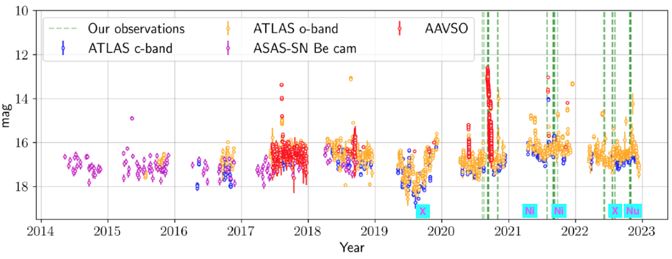
Figure 1: Long-term optical lightcurve of CJ2056, overlaid with the SALT observations indicated by vertical, dashed green lines. The XMM-Newton, NICER  and NuSTAR observations are denoted by ”X,” ”Ni,” and ”Nu” cyan boxes on the bottom.

CJ2056 was observed in the X-ray band five times between 2019 and 2022 (Table 2). Figure 1 shows the optical light curve of CJ2056 over the last decade, overlaid with all X-ray observation dates. Besides the routine optical monitoring provided by ASSASN (ASS1; ASS2), ATLAS (atl), and AAVSO aavso, dedicated optical observations at SAAO were conducted and reported in our companion paper (van Dyk et al.).

CJ2056 was observed by XMM-Newton twice on October 24, 2019 (18 ks; Oliveira) and on October 23, 2022 (54 ks). The source extraction region was a circle of $r=20^{\prime\prime}$ around the source position, while an annular region of $r=30\rm{-}50^{\prime\prime}$ was used for background extraction. All XMM-Newton data sets were reduced using SAS 19.1, using emchain and epchain for GTI filtering for MOS and pn modules, respectively, with evselect for region extraction (2004ASPC..314..759G). The 2019 observation yielded 0.3–10 keV count rates of 0.103, 0.096, and 0.429 cts/s for the MOS1, MOS2, and pn modules, respectively. Meanwhile, the 2022 observation yielded count rates of 0.108 (MOS1), 0.110 (MOS2) and 0.528 (pn) cts/s. We collected $\sim 13,000$ and $\sim 40,000$ net counts for MOS and pn data in 0.3–10 keV after combining the 2019 and 2021 XMM-Newton observation data.

CJ2056 was observed by NICER for 53 ks exposure on July 25, 2021. NICER observations were again performed on November 6, 2021, with 20 ks of total exposure. Both data sets were reduced using nicerl2, which generates cleaned and reduced event and spectrum files. Background model spectra were produced using nibackgen3C50 (3c50). The NICER observations yielded $\sim 67,000$ and $\sim 25,000$ total counts in the 0.5 - 1.5 keV band, resulting in count rates of 1.27 and 1.22 cts/s, respectively, beyond which background events dominated.

A 21 ks NuSTAR observation was conducted on November 4, 2022. We processed the NuSTAR data using nupipeline (Harrison2013). We extracted source events from a $r=30^{\prime\prime}$ circular region around the target position. An annular region at $r=100\rm{-}180^{\prime\prime}$ was used for extracting background events. The NuSTAR data, with FPMA and FPMB module events combined, yielded $\sim$ 3,700 net counts in the 3–30 keV band after background subtraction, with respective count rates of 0.088 and 0.082 cts/s. We found that the NuSTAR data were heavily contaminated by background photons above 30 keV.

Table 2: X-Ray observation log of CJ2056

Date	ObsId	Telescope	Exposure (ks)
2019-10-24	0842570101	XMM-Newton ${}^{1}$	18
2021-07-25/29	459201020*	NICER	53
2021-11-05/06	459201030*	NICER	20
2022-10-23	0902500101	XMM-Newton ${}^{1}$	54
2022-11-04	30801006002	NuSTAR	21

${}^{1}$ This observation was carried out in Prime-Full Window Mode
${}^{*}$ NICER observations are collected in several successive observations sharing the same obsID prefix

3 Timing Analysis

All X-ray observation data were analyzed with the Stingray software package (matteo_bachetti_2022_6394742) and Hendrics (hendrics) for our timing study. First, we applied barycentric correction to all extracted source events. The SAS command barycen was used for the 2019 and 2022 XMM-Newton data. MOS 1 and 2 data were combined for timing analysis. Meanwhile, the NICER and NuSTAR source events were corrected with the barycorr command from HEASOFT Version 6.25 (heasoft). We applied energy filtering using Hendrics command-line tools.

3.1 Periodicity search

We began our analysis with the $H$-test for $n=1,2,3$ harmonic components using the weighted $Z^{2}_{n}$ function through z_n_search in Stingray. Our periodicity search swept over a frequency range of $f=10^{-3}\rm{-}10^{2}$ Hz using the reciprocal of the observation length as the frequency step size for each dataset, yielding the most significant detections ($>\;7\sigma$ significance) of the 29.6 sec spin period at $n$=3 in the XMM-Newton and NICER observations. The significance and false-alarm probabilities of the peak signals presented account for the number of trials which is given by the length of the frequency range divided by the frequency step-size of each search. In the XMM-Newton periodograms, sub-harmonic signals are present. Using fewer harmonic components, i.e., $n=1$ and $n=1,2$ resulted in detecting the spin period at similar significance (e.g., for the first NICER observation, $Z^{2}_{1}=989.29$ and $Z^{2}_{2}=1019.96$), without additional sub-harmonic signals. Meanwhile, we detected the spin signal in the NICER observations in the same energy band (0.3–2 keV). Due to aperiodic variability, we did not detect its sub-harmonic with NICER  regardless of how many harmonics were summed.

At higher energy bands above 2 keV, the spin period was more weakly detected in the XMM-Newton and NICER data; the significance of the peak signal of the $Z^{2}_{1}$ searches for each dataset never exceeded $4-\sigma$. As the $Z^{2}$ statistic of the peak frequency was only negligibly increased by summing out to three harmonics, we used the $Z^{2}_{1}$ test in a narrower frequency band ($f=5\rm{-}50$ mHz) around the spin period to characterize the peak and its uncertainty without the spurious subharmonics (Figure: 2). In the narrow-band $Z^{2}$ data, we fit the 29.6-sec peak with a Gaussian function and found its width of $\Delta f<0.007$ mHz. The frequency resolution is consistent with the Nyquist limit corresponding to a reciprocal of the observation length. Later, we constrained the spin period more accurately based on the two NICER observations as NICER provides better temporal resolution ($<\mu$s) than XMM-Newton.

We performed the same timing analysis above 3 keV using the NuSTAR data. As we performed the $Z^{2}_{1}$ test in the same frequency band ($f=5\rm{-}50$ mHz) as the XMM-Newton timing analysis, we found that a peak at the spin period was detected at the 4.0$-\sigma$ level. (Figure 4).

Table 3 summarizes all of our spin period measurements. While our results are consistent with the 2019 XMM-Newton observation findings (Oliveira), joint NICER data analysis from the two observations separated by $\sim$ 3 months reduced the spin period uncertainty significantly compared to the XMM-Newton results.

3.2 Folded X-ray lightcurves and hardness ratio profiles

Following the spin period detection, we produced pulsed profiles folded at 29.6 sec for each X-ray observation. Although no significant periodicity was detected above 2 keV, we generated folded lightcurves in the 0.3–2 keV and 2–10 keV bands, using Stingray’s fold_events with 20 bins per cycle. The pulse fraction, as defined by stingray is $\frac{a-b}{\mathrm{x}}$, where $a$ and $b$ are the minimum and maximum of the profile and $x$ is the mean counts across the phase bins (matteo_bachetti_2022_6394742). The soft X-ray profiles exhibit a single broad peak with a pulse fraction between 15 % and 25 % (Table 3). The spin modulation was more prominent in the XMM-Newton observations than the NICER observations, which were subjected to higher background contamination and thus a higher mean counts compared to the amplitude of modulation (Figure 3). With the NuSTAR data, we generated a 3–10 keV pulsed profile folded over the 29.6 sec period and found modulation with a pulse fraction of 16.2 %. We also produced X-ray lightcurves folded by $P=59.2$ sec, which exhibit two symmetric non-overlapping pulses. It establishes that the 29.6 s signal represents the fundamental spin period, confirming the results of Oliveira.

Using the XMM-Newton pn data from both XMM-Newton observations, we generated hardness ratio curves folded over the 29.6-sec spin period with 20 phase bins. We compared the source counts between the 2–5 keV and 0.3–2 keV. The hardness ratio curves for the 2019 and 2022 XMM-Newton observations demonstrated only weak modulations (Figure 5) possibly correlated with the X-ray flux modulation – the X-ray emission became softer when the source was brighter. For better visualization, we overlaid the best-fit sinusoidal functions in the hardness ratio curves and the 3-$\sigma$ significance lines deviating from the mean hardness ratios. The sinusoidal function fit to the 2019 data had an amplitude of $N=0.013\pm 0.006$ with $\chi^{2}_{\nu}$ = 0.64 for 18 degrees of freedom (d.o.f.). Then, the spin modulation of the hardness ratio is not significant. The fit to the 2022 XMM-Newton data, with nearly four times more source counts, produced $\chi^{2}_{\nu}$ = 0.95 for 18 d.o.f. with amplitude $N=0.009\pm 0.004$. This observation was less contaminated by background events, and the spin signal appeared with more than 3 times the $Z^{2}_{1}$ power in the new XMM-Newton observation. In this extended observation, we detected hardness ratio modulation at 3-$\sigma$.

3.3 The spin period stability and derivative

To investigate the stability of the spin period, we created dynamical power spectra in 0.3–2 keV from the XMM-Newton pn observation data in 2022, as it provides the longest net exposure time and the longest continuous intervals of observation in this energy band among all X-ray observations (Figure 6 right panel). We found that the 29.6-sec spin period was stable during the 54 ks X-ray observation in contrast to the occasional variability of the WD spin observed in the optical band (van Dyk et al. in prep).

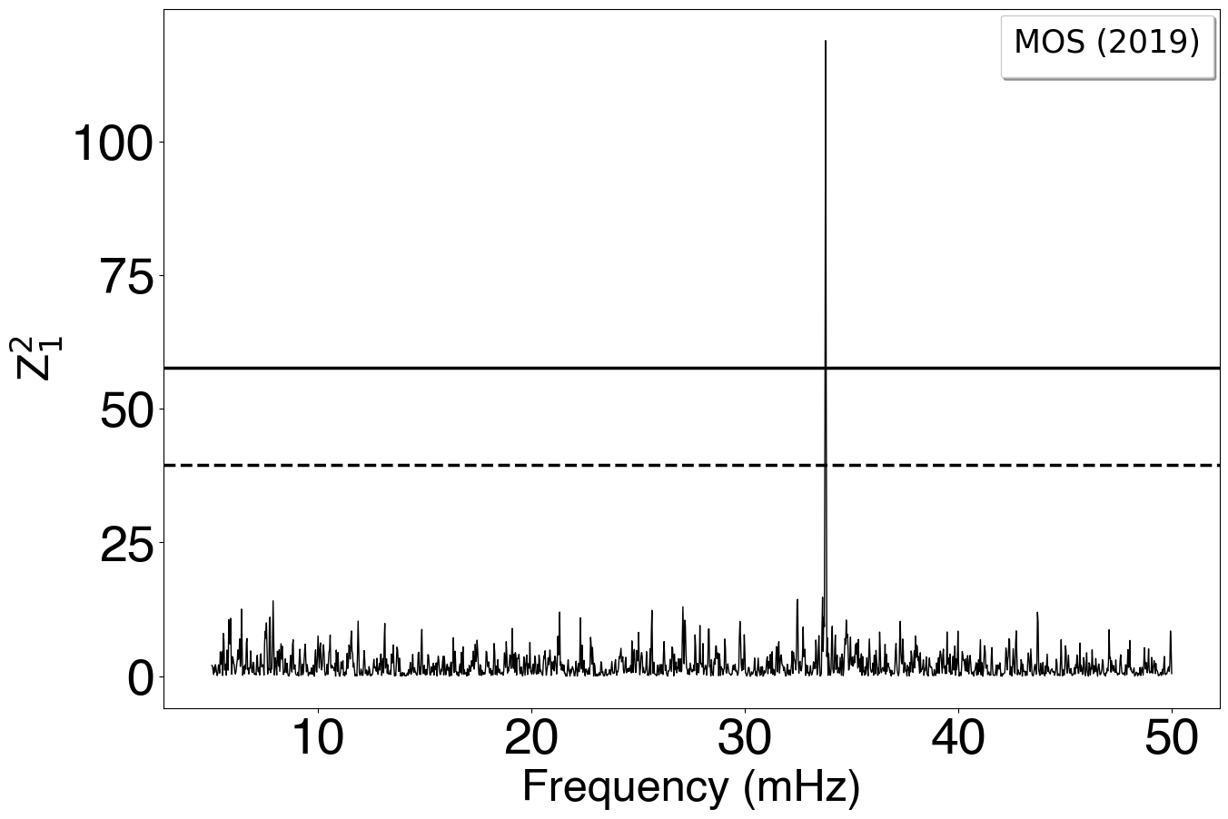
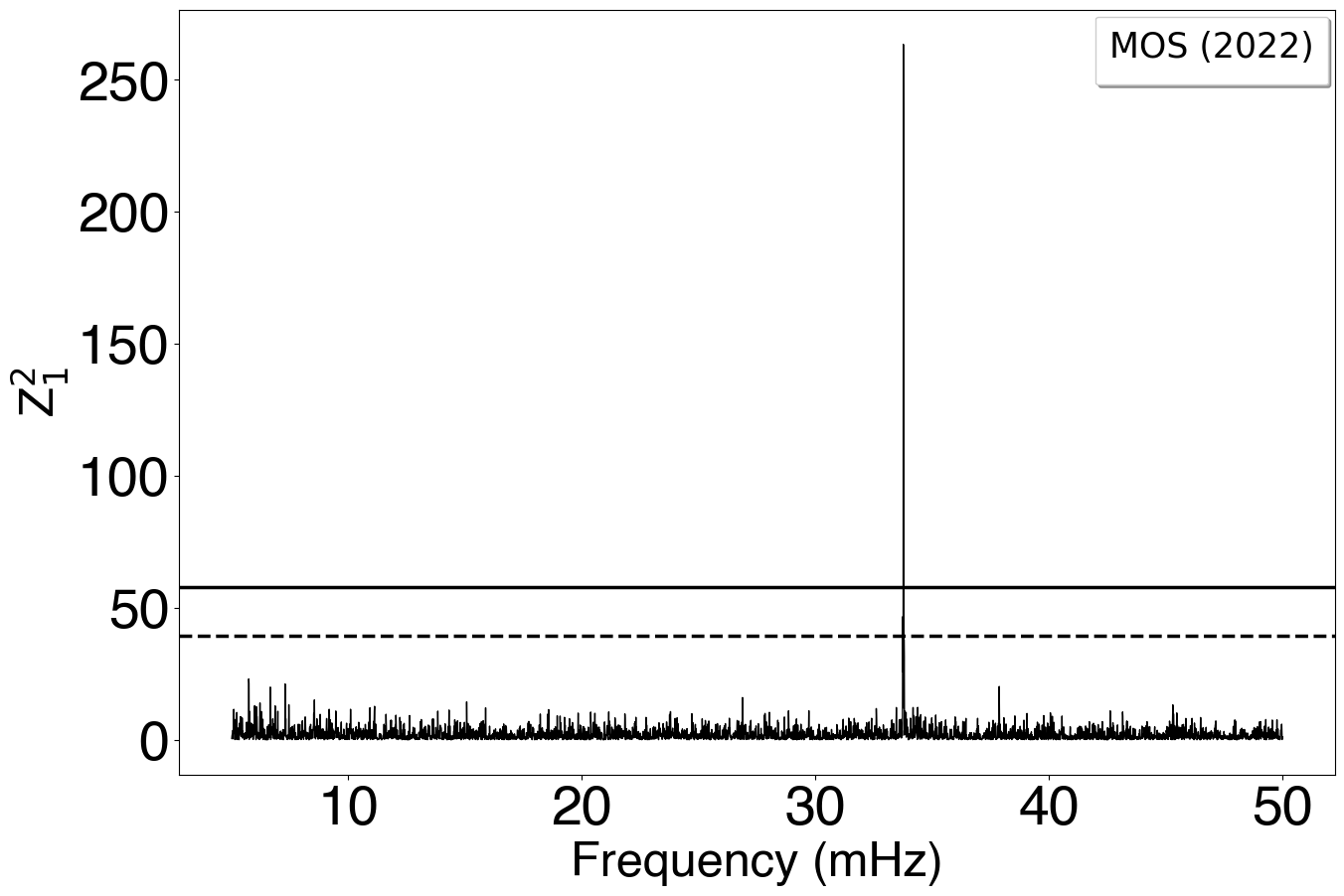
Figure 2: $Z^{2}_{1}$ soft X-ray (0.3 - 2 keV) periodograms. The top row from left to right: 0842570101 MOS, 459201020* NICER, and 0902500101 MOS. The bottom row from left to right: 0842570101 pn, 459201030* NICER, and 0902500101 pn. In each periodogram, 3-$\sigma$ and 5-$\sigma$ significance levels are shown by solid and dashed lines, respectively. The most significant peak is in the region of P $\sim$ 29.6 seconds. While the 5 mHz to 25 mHz range is excluded from the NICER periodograms due to substantial aperiodic variability, for the XMM observations, the harmonic of the 29.6 sec signal is highly significant at 59.2 seconds.

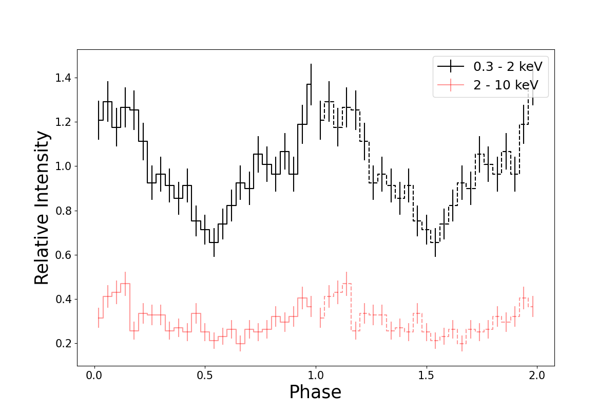
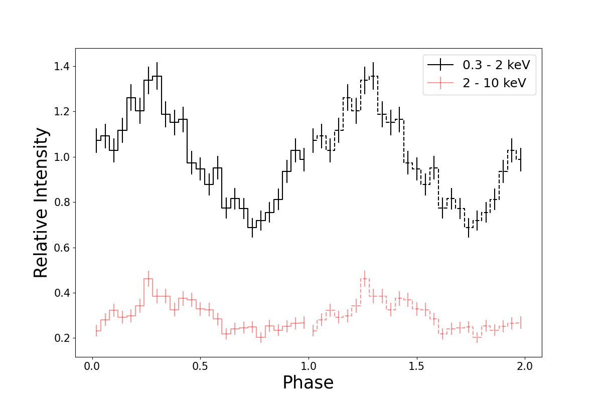
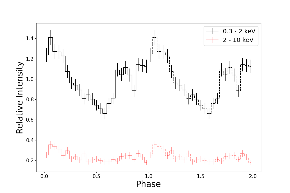
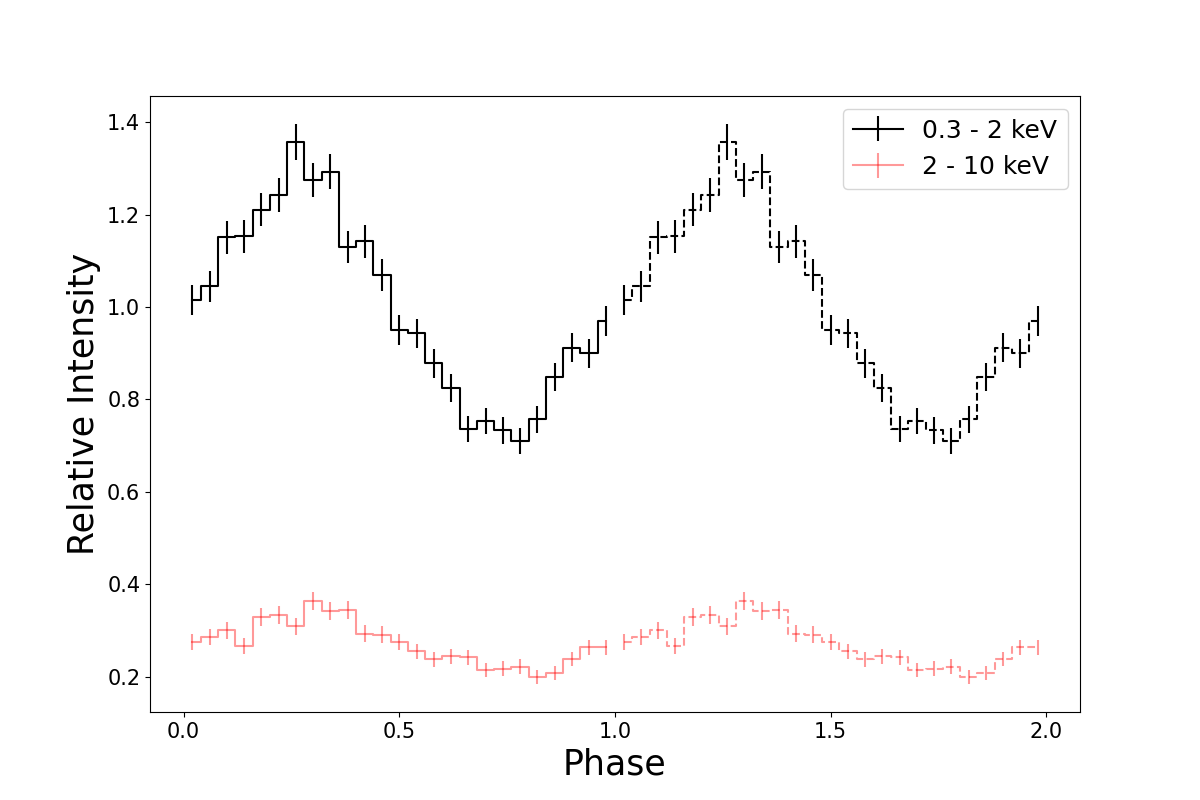
Figure 3: Pulse profiles of folded source events in the soft (0.3 - 2 keV) and hard (2 - 10 keV) X-ray band. he top row from left to right: 0842570101 MOS, 459201020* NICER, and 0902500101 MOS. The bottom row from left to right: 0842570101 pn, 459201030* NICER, and 0902500101 pn. Relative intensity is defined as the fraction of the mean count rate of the soft X-ray profile. 1-$\sigma$ error bars are included.

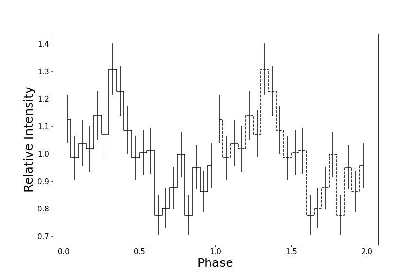
Figure 4: Left:30801006002 FPMA+FPMB joint $Z^{2}_{1}$ search (5 mHz - 50 mHz). The 3-$\sigma$ and 5-$\sigma$ significance levels are shown by solid and dashed lines, respectively. Right: The pulse profile of the folded NuSTAR events at 29.6 sec. Relative intensity is defined by the mean count rate of the folded events. 1-$\sigma$ error bars are included.

Figure 5: The hardness ratio folded at 29.6 sec with 20 bins per cycle for the 2019 pn (left) and 2022 pn (right) observations. The dotted lines represent the 3-$\sigma$ significance line for deviation from the mean. Overlaid are the best-fit sinusoidal curves in black. In blue, we present the folded light curve of each observation in the 0.3 - 5 keV band to demonstrate the anticorrelation between the hardness ratio and the luminosity.

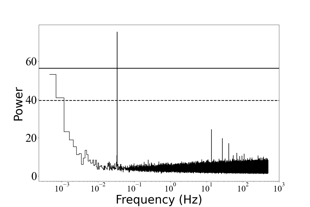
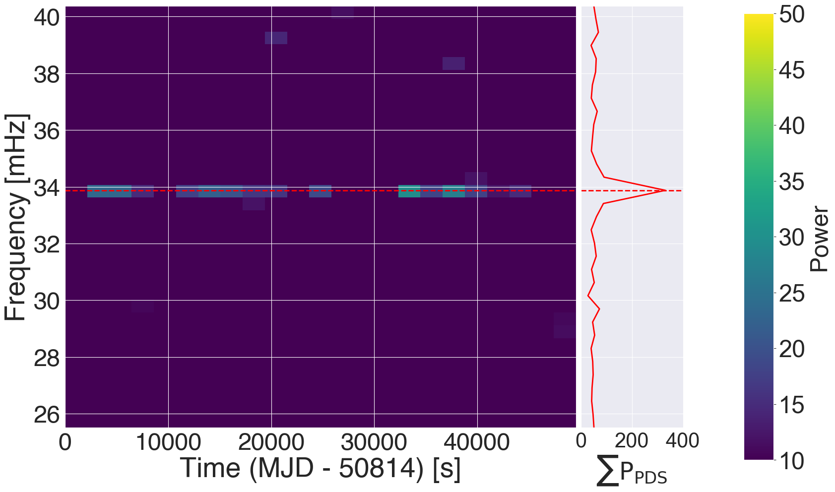
Figure 6: Left: A PDS periodogram obtained from the 2022 XMM-Newton-pn data in the 0.3 - 2 keV band, demonstrating a strong peak at $f\sim 33.7\,\mathrm{mHz}$. The 5-$\sigma$ and 3-$\sigma$ significance lines are shown by the solid and dashed lines, respectively. Right: 2022 XMM-Newton -EPIC pn dynamical power spectrum periodogram. The measured peak from the PDS is shown in green.

Figure 7: The results of the demodulation analysis on the combined NICER observations. The color-scale representation shows the peak frequency’s power change as a function of demodulation amplitude (A) and phase ($\phi$). The highest $Z^{2}_{1}$ value, marked by ’x,’ indicates the most significant spin period detection, giving the best fit A and $\phi$. The black lines show the 1, 2, and 3-$\sigma$ significance contours.

Based on the two NICER observations (separated by $\sim$ three months) with 70 ks total exposure in 2021, we attempted to constrain the spin period evolution of CJ2056. The NICER data provides the most accurate timing data given its superb resolution ($0.3<\mu$s). Following Makishima2021, we employed a demodulation method to consider the orbital motion. For all photon event arrival times with respect to the reference time 01/01/1998 00:00:00 UTC, we fit $\Delta t=A\sin\left(\frac{2\pi t}{P_{\rm orb}}+\phi_{0}\right)$ where $P_{\rm orb}=1.76$ hr (orbital period), $A$ is an amplitude and $\phi_{0}$ is a phase shift. $A$ and $\phi_{0}$ are the two unknown parameters we varied to calculate the confidence level contours shown in Figure 7. The demodulation parameters should be constant across all observations. Using both NICER observation data, we constrained $A<1.5$ [s] and found that $\phi$ is unconstrained. Our results suggest that the effects of orbital modulation may be intrinsically small (e.g., possibly due to a face-on view of the orbital plane) or we need more high-resolution X-ray timing data over a longer baseline. Either way, the orbital modulation does not significantly contribute to determining the spin period’s uncertainty in the current X-ray data. By adopting $A<1.5$ [s] and using all NICER observation data (with 73 ks total exposure over 104 days), we determined the spin period most accurately ($P=29.6089\pm 0.0002$ s) among the previous timing studies presented in Oliveira. We applied the best orbital parameters ($A<1.5$ [s] for a range of $\phi=0\rm{-}1$) to XMM-Newton pn data in 2019 and 2022. We performed joint $Z^{2}_{2}$ tests with the XMM-Newton pn and NICER timing data spanning over three years, assuming a non-zero spin derivative. We found no significant period difference and derived an upper limit of the spin period derivative of $|\dot{P}|<1.8\times 10^{-12}$ s/s with 90 % confidence.

Table 3: Summary of Timing Analysis

Instrument	Peak frequency [mHz]	Peak period [sec]	Counts	$Z^{2}_{1}$	False Alarm Probability${}^{b}$	$P$ [%]${}^{a}$
XMM-Newton 0.3–2 keV
0842570101
MOS	33.78(3)	$29.61(1)$	3890	118.82	$2.5\times 10^{-23}$	25(1)
pn	33.78(3)	$29.61(2)$	6350	200.8	$3.5\times 10^{-41}$	27(1)
0902500101
MOS	33.77(1)	29.609(5)	9142	263.37	$3.1\times 10^{-54}$	24.3 (9)
pn	33.77(1)	29.608(6)	22,853	814.64	$5.8\times 10^{-174}$	27.9 (5)
NICER 0.3–2 keV
459201020*	33.773(1)	29.6095(8)	87,105	989.29	$1.1\times 10^{-212}$	15.5(3)
459201030*	33.772(5)	29.610(4)	35,824	484.98	$9.2\times 10^{-104}$	16.8(4)
Joint	33.7735(3)	29.6089(2)	122,929	974.35	$1.9\times 10^{-209}$	14.9(2)
NuSTAR 3–10 keV
30801006002
FPMA + FPMB	33.767(7)	29.614(6)	2966	37.11	$4.7\times 10^{-5}$	16.2(1.8)

All errors shown are at 90% confidence intervals. The uncertainty on the last digit of peak frequency, peak period, and pulse fraction is shown in parentheses next to the observed value. The results are from the $Z^{2}_{1}$ test in the narrow frequency band. The total counts for each observation, instrument, and energy band are also listed.

${}^{a}$Pulsed fractions [%] and upper limits were calculated by HENzsearch (matteo_bachetti_2022_6394742).

${}^{b}$ The false alarm probability, the probability that the peak signal was generated by noise, was calculated with Stingray function z2_n_probability.

4 Spectral Analysis

We jointly fit the XMM-Newton and NICER spectra with phenomenological models. The NuSTAR observation saw a substantial flux enhancement that coincided with an increase in optical flux. However, it is uncertain if this event represents a dwarf nova outburst (van Dyk et al., in preparation). The unabsorbed X-ray flux was measured to be $F_{X}=7.6\times 10^{-12}\;$ ergs s${}^{-1}$ cm${}^{-2}$ in the 0.3 - 12 keV band, a factor of four greater than all other observations with $F_{X}\sim 2\times 10^{-12}\;$ ergs s${}^{-1}$ cm${}^{-2}$ . Thus, we fit its data separately. Various combinations of X-ray absorption and thermal plasma spectral components were applied. Due to the improved photon statistics over the previous X-ray study (Oliveira), we could perform a phase-resolved X-ray spectral analysis and search for the spin variation.

4.1 Phase-Averaged Spectral Analysis

For the phase-averaged spectral analysis, phenomenological models were fit to the joint XMM-Newton and NICERX-ray spectra and NuSTAR X-ray spectra to characterize the X-ray spectral properties further and expand upon the analysis previously presented by Oliveira. All spectral fittings were performed using XSPEC version 12.13.1 (Arnaud1996). Each spectral model included tbabs to account for ISM absorption using the Wilms abundance data (Wilms2000). Furthermore, constant is included as a cross-normalization factor between different observations in the joint fit. We set the constant factor to 1 for the earliest XMM-Newton observation in 2019.

Table 4: Phenomenological model fits to X-ray spectra

Parameter	pow${}^{e}$	APEC${}^{e}$	$2\cdot$APEC	pow + $2\cdot$APEC	bbody + $2\cdot$APEC	$3\cdot$APEC	$3\cdot$APEC + gauss
$C_{XMM}^{a}$	$0.84\pm 0.02$	0.83	$0.83\pm 0.02$	0.83 $\pm 0.02$	0.83 $\pm 0.02$	$0.83\pm 0.02$	$0.83\pm 0.02$
$C_{2021}^{a}$	$1.09\pm 0.02$	1.10	$1.06\pm 0.02$	$1.02\pm 0.02$	$1.03\pm 0.02$	$1.03\pm 0.02$	$1.03\pm 0.02$
$C_{2022}^{a}$	$1.23\pm 0.03$	1.25	$1.19\pm 0.03$	$1.15\pm 0.03$	$1.16\pm 0.03$	$1.16\pm 0.03$	$1.16\pm 0.03$
$N^{(i)}_{H}(10^{20}\rm{cm}^{-2})^{b}$	$15.5\pm 0.5$	4.99	$1.4\pm 0.3$	9.2 $\pm 0.9$	6.2 $\pm 1.0$	$4.2_{-0.5}^{+0.6}$	$4.2\pm 0.6$
$\Gamma$	$2.44\pm 0.04$	…	…	1.6 $\pm 0.1$	…	…	…
$kT_{1}$ (keV)	…	2.13	$0.85\pm 0.01$	$0.30_{-0.01}^{+0.02}$	0.18$\pm 0.01$	$0.30\pm 0.01$	$0.33\pm 0.01$
$kT_{2}$ (keV)	…	…	$4.39_{-0.18}^{+0.16}$	$1.12\pm 0.02$	$0.94\pm 0.02$	$1.01_{-0.02}^{+0.03}$	$1.01_{-0.02}^{+0.03}$
$kT_{3}$ (keV)	…	…	…	…	$6.35_{-0.50}^{+0.73}$	$4.90_{-0.23}^{+0.22}$	$4.86\pm 0.23$
$Z^{c}(Z_{\odot})$	…	0.07	$0.51\pm 0.06$	$0.13_{-0.03}^{+0.08}$	$0.57_{-0.09}^{+0.10}$	$0.53_{-0.06}^{+0.07}$	$0.52_{-0.06}^{+0.07}$
$E_{\rm line}$ (keV)	…	…	…	…	…	…	6.4
$\sigma_{\rm line}$ (keV)	…	…	…	…	…	…	0.01
$EW_{\rm line}$ (eV)	…	…	…	…	…	…	$<73$
$F_{X}(10^{-12}\frac{\mathrm{erg}}{\mathrm{cm}^{2}\mathrm{s}})^{d}$	2.51	3.36	6.72	8.19	7.72	7.04	7.09
$\chi^{2}_{\nu}$ (dof)	1.93 (2330)	2.18 (2329)	1.16 (2327)	1.06 (2325)	1.06 (2325)	1.01 (2325)	1.01 (2324)

All errors shown are $90\%$ confidence intervals.
${}^{a}$ Cross-normalization factors of the XMM-Newton data in 2022 ($C_{XMM}$), and the NICER data in 2021 ($C_{2021}$) and 2022 ($C_{2022}$) with respect to the XMM-Newton observation in 2019.
${}^{b}$ The ISM hydrogen column density associated with tbabs which is multiplied to all the models.
${}^{c}$ Abundance relative to solar.
${}^{d}$ 3 – 10 keV flux of the XMM-Newton pn (2019) data.
${}^{e}$ Reduced $\chi^{2}$ is too great to calculate error.
${}^{*}$ The parameter is frozen.

Table 5: Phenomenological Model Fits to the NuSTAR spectra

Parameter	pow${}^{e}$	APEC${}^{e}$	APEC + gauss
$N^{(i)}_{H}(10^{20}\rm{cm}^{-2})^{a}\;*$	$4.2$	4.2	4.2
$\Gamma$	$2.27\pm 0.06$	…	…
$kT_{1}$ (keV)	…	$8.2_{-0.5}^{+0.6}$	$8.4_{-0.6}^{+0.7}$
$Z^{b}(Z_{\odot})$	…	$0.40_{-0.11}^{+0.13}$	$0.32_{-0.12}^{+0.13}$
$E_{line}$ (keV)*	…	…	6.4
$\sigma_{line}$ (keV)*	…	…	0.01
$EW_{line}$ (eV)	…	…	$174_{-76}^{+75}$
$F_{X}(10^{-12}\frac{\mathrm{erg}}{\mathrm{cm}^{2}\mathrm{s}})^{c}$	4.21	4.39	4.39
$\chi^{2}_{\nu}$ (dof)	1.36 (256)	1.05 (255)	0.99 (254)

All errors shown are $90\%$ confidence intervals.
${}^{a}$ The ISM hydrogen column density associated with tbabs, which is multiplied to all the models.
${}^{b}$ Abundance relative to solar.
${}^{c}$ 3 – 10 keV flux of the NuSTAR data.
${}^{*}$ The parameter is frozen.

Fitting an absorbed power-law model to the joint spectrum resulted in a poor fit to the data ($\chi^{2}_{\nu}=1.93$), largely due to atomic lines at 6.7–7 keV, indicating that the X-ray emission is thermal. We applied an emission spectrum model (APEC) that accounts for the emissions from collisionally-ionized diffuse gas due to accretion. A single temperature APEC model did not fit the data well ($\chi^{2}_{\nu}=2.18$) with the best-fit temperature of $kT=3.37$ keV. We then fit an absorbed 2-temperature model (APEC+APEC). The fit was significantly improved ($\chi^{2}_{\nu}=1.16$) with the best-fit temperatures $kT=0.85$ and 4.39 keV. Despite the improvement, the model failed to fit the X-ray spectra above 6–7 keV accurately. We added a third APEC model with a higher plasma temperature. The 3-temperature model (APEC+APEC+APEC) yielded a better fit with $\chi^{2}_{\nu}=1.01$ with the best-fit temperatures $kT=0.30,1.01$ and 4.90 keV. Some residuals are present below 2 keV, possibly due to complex X-ray absorption often seen in IPs (Mukai2021). The abundance ($Z$) was linked between the different APEC components and we found $Z=0.54_{-0.06}^{+0.07}\;Z_{\odot}$ for the 3-T model.

We also considered a combination of thermal and power-law components (e.g., APEC+APEC+PL). However, the fit was not improved ($\chi^{2}_{\nu}=1.06$) compared to the thermal-only models. Thus, we conclude that there is no evidence of non-thermal X-ray emission based on the broadband X-ray data. Although the lower-energy residuals improved, the fit was again poor in the region of the hard X-ray photons. We also replaced the lowest temperature APEC model with a blackbody model by fitting an absorbed BBODY+APEC+APEC model. The fit quality was again similar to the thermal and power-law model ($\chi^{2}_{\nu}=1.06$) and the best-fit blackbody temperature was 0.18 keV. The soft blackbody component could originate from the base of the accretion column as observed from other mCVs (Ramsay_2002).

In IPs, some X-rays emitted from the accretion column can be reflected by the WD surface or absorbed by the accretion curtain. These effects cause a neutral Fe K-$\alpha$ fluorescence line at 6.4 keV and complex X-ray absorption at lower energies (Mukai2021). Following previous X-ray studies (e.g., Hailey2016), we added a Gaussian line component at $E=6.4$ keV to the absorbed 3-T APEC model to account for the neutral Fe K-$\alpha$ fluorescence line. We fixed the line energy and set the line width to $\sigma=0.01$ keV. The fit improved by only $\Delta\chi^{2}=1.3$ over 2325, indicating that adding the Gaussian component is not statistically significant. We found a 3–$\sigma$ upper limit of the Gaussian component to EW $<79$ eV. The other spectral parameters remained nearly unchanged from the fit without the Gaussian line component. From these fits, we constrained $n_{H}$ to $4.2\pm 0.6\times 10^{20}\;\rm{cm}^{-2}$. The best-fit absorbed flux was $7\times 10^{-13}\;$ergs s${}^{-1}$ cm${}^{-2}$(Table 4).

As the X-ray spectrum of CJ2056 extends down to 0.3 keV, X-ray absorption seems insignificant. We added a partial covering absorption component (pcfabs), which accounts for X-ray absorption in the accretion curtain for IPs (Hailey2016). However, it did not improve the spectral fits in any of the aforementioned cases.

For the NuSTAR spectrum, we froze $n_{H}=4.2\times 10^{20}\;\rm{cm}^{-2}$ as the lack of counts left the value otherwise unconstrained. Here, the absorbed power-law model also fit poorly due to the atomic lines in the 6.7 - 7 keV region ($\chi^{2}_{\nu}=1.36$). A single temperature APEC model improved the fit to $\chi^{2}_{\nu}=1.05$. The highest temperature component of the XMM-Newton and NICER fits (formerly 4.9 keV) is better characterized by a temperature of 8.4 keV in the broader 3 - 30 keV energy band. Adding a Gaussian component to account for the neutral Fe line further improved the fit to $\chi^{2}_{\nu}=0.99$, increasing temperature to 8.4 keV and decreasing the abundance to $Z=0.32_{-0.12}^{-0.13}M_{\odot}$. The EW of the Gaussian component ($174_{-76}^{+85}$ eV) was substantially stronger here than in the joint fitting, which weakly indicated the presence of an Fe line. A partial covering absorption component, however, similarly did not improve the fit to the ${\it NuSTAR}$ observation. Finally, we fit best-fit $3\cdot$APEC + gauss model from the XMM-Newton and NICER observations, freezing all components of the model except for normalization factors. The fit was poor with $\chi^{2}_{\nu}=1.66$ for 254 d.o.f. with prominent residuals in the above 7 keV, confirming that the X-ray spectrum has hardened during the outburst that NuSTAR observed.

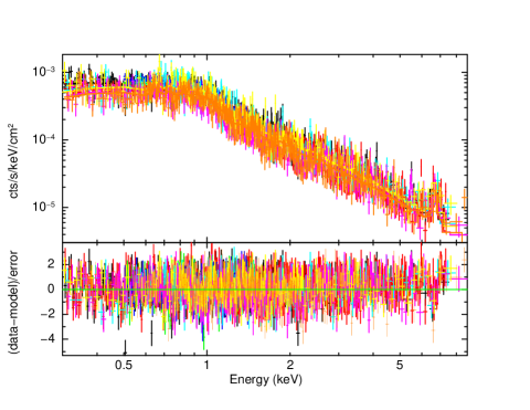
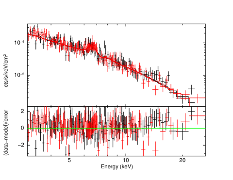
Figure 8: Left: XMM-Newton  NICER spectra and residuals of CJ2056 fit with an tbabs*(APEC+APEC+APEC + gauss) model, which yielded a $\chi^{2}_{\nu}=1.01$ for 2324 degrees of freedom. The 2019 XMM-Newton observation (obsID = 0842570101) is presented in the 0.3 - 10 keV band with MOS1 in cyan, MOS2 in yellow, and pn in black. Similarly, 2022 XMM-Newton observation (obsID = 0902500101) is presented in the 0.3 - 10 keV band with MOS1 in magenta, MOS2 in orange, and pn in red. The NICER observations are presented in the 0.5 - 1.5 keV band, with obsID = 459201020* in green and obsID = 459201030* in blue. Right: NuSTAR spectrum and residuals fit with a tbabs*APEC, which yielded a $\chi^{2}_{\nu}=0.99$ for 254 degrees of freedom. The NuSTAR observation is presented in the 3-30 keV band, with FPMA in black and FPMB in red.

4.2 Phase-Resolved Spectral Analysis

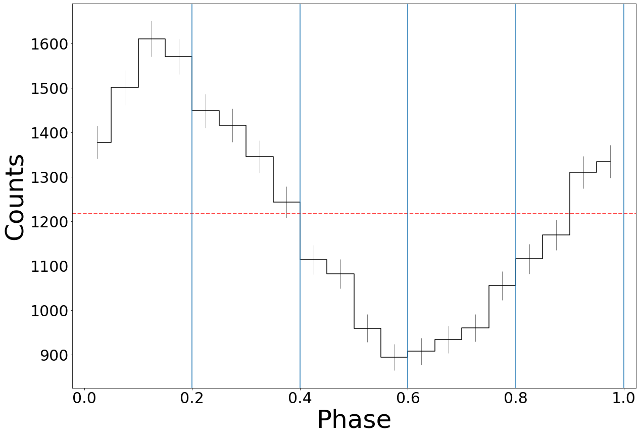
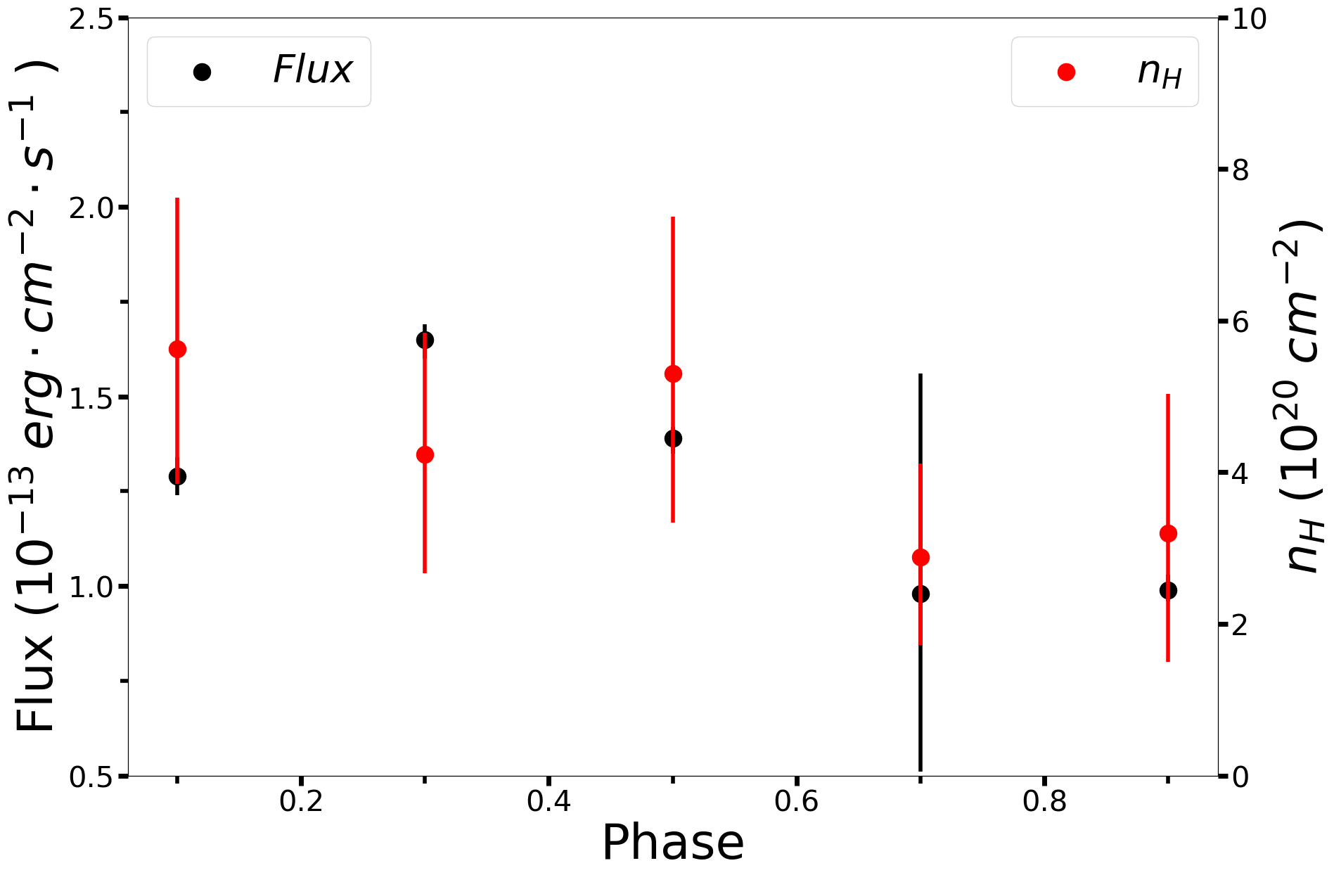
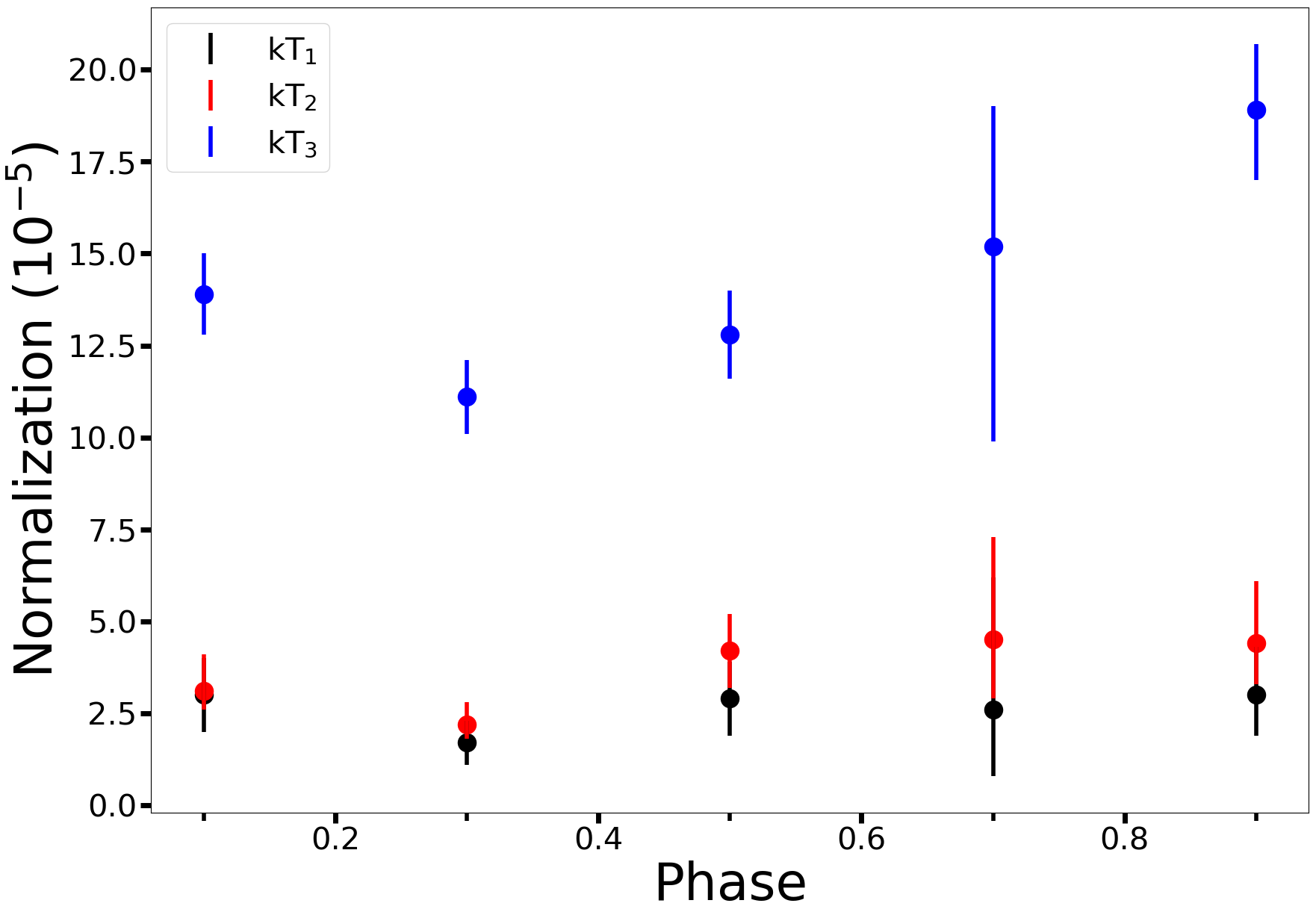
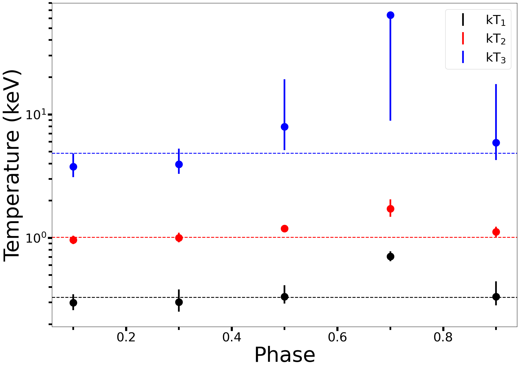
Figure 9: Top Left: The 2022 EPIC-pn light curve folded at the peak spin period, demonstrating the phase bins the spectra were cut into. The dotted red line denotes the mean counts, while the blue lines mark the 5 phase intervals ($\phi=0.0\rm{-}0.2,0.2\rm{-}0.4,0.4\rm{-}0.6,0.6\rm{-}0.8$ and 0.8–1.0), where XMM-Newton spectra were separately fitted. Top Right: The soft X-ray (0.3 - 2 keV) flux plotted against the fitted $n_{H}$ across the phase bins with all temperatures fit freely. It can be observed that fitted absorption decreases in the brightest bins. Bottom: The flux normalization variation and plasma temperature variation for each APEC component across five phase intervals. For comparison, the phase-averaged values are shown as dotted lines. The phase-resolved spectroscopy demonstrated a change in normalization that similarly affects all three single temperature components of the model. The fourth phase bin at $\phi=0.6\rm{-}0.8$ shows a substantial, but poorly constrained, spectral hardening that is pronounced across all temperature components.

We performed phase-resolved spectral analysis using the best-fit spin period. As IPs often demonstrate energy-dependent spin modulation, CJ2056 may demonstrate some phase variation in its X-ray spectra (1988Rosen, Joshi2022). We calculated phase values for all source photon events based on each observation’s best-fit spin period ($P=29.61$ s). We extracted X-ray spectra from five phase intervals with equal length ($\Delta\phi=0.2$; Figure 9 left panel). The NICER data was excluded from the phase-resolved spectral analysis due to the lack of source counts in the energy band above 1.5 keV. We also exclude the NuSTAR data as it is described best by a different model than the other observations. We refrain from presenting its own phase-resolved spectroscopy due to insufficient counts (a few hundred per phase bin) and the unconstrained $n_{H}$ in this energy band.

We fit each phase-resolved spectrum with an absorbed 3-temperature model constant*tbabs*(APEC+APEC+APEC), varying all parameters, except for the abundance which was frozen to the phase-averaged best-fit abundance. The fit quality was excellent for the first three bins with $\chi^{2}_{\nu}$ between 0.95 and 1.01. However, phase bins 4 and 5 contained the least bins and worst fits ($\frac{\chi_{\nu}^{2}}{\nu}=\frac{0.91}{401}$ and $\frac{\chi_{\nu}^{2}}{\nu}=\frac{0.89}{434}$). This also led to poor constraints of the fit parameters, particularly the highest temperature component, in phase bin 4. The source undergoes spectral hardening at its spin-phase flux minima (in phase bins 3 and 4), particularly in its lower temperature components, as demonstrated by the increase in $kT_{1}$ and $kT_{2}$, while $kT_{3}$ is unconstrained. We also present the flux variability in the 0.3–2 keV range, where the spin-period signal was significantly detected. Again, the soft component of the X-ray spectrum reaches a maximum at the flux maximum. This result confirms the behavior demonstrated by the hardness ratio modulation. Meanwhile, the X-ray absorption, quantified by $n_{H}$, shows a weak anti-correlation with soft X-ray flux. To avoid degeneracy between flux normalization and the fitted temperature of each component, we compared the relationship between flux and $n_{H}$ with frozen $kT_{1}$, $kT_{2}$, and $kT_{3}$ but found the same behavior.

5 White Dwarf Mass Measurement

In general, X-ray emission in CVs is powered by mass accretion, converting the gravitational potential energy of incoming particles to X-rays by radiative cooling via the shock-heated gas flow. In non-magnetic CVs (nmCVs), the accretion disk tends to approach the WD surface, where a boundary layer is formed and dissipates most of the gravitational energy into X-ray emission. In magnetic CVs (mCVs), accreting material is funneled onto the WD poles along the magnetic field lines. It forms a column of infalling gas, which is first heated by a standoff shock and then cools toward the WD surface by producing thermal X-ray emission (Mukai2017). In either case, X-ray spectra exhibit multi-temperature components, either due to the boundary layer or accretion flow with varying plasma temperature and density profiles. X-ray emission from nmCVs and mCVs has been well studied, both observationally and theoretically, and can be used to determine WD mass (e.g., Shaw2020). While Oliveira suggested CJ2056 is an IP and thus its X-ray emission results from a tall accretion column, the detection of dwarf novae could indicate that the WD may be weakly magnetized like nmCVs. Given that the nature of CJ2056 is unknown, we considered both the nmCV and mCV cases to determine the WD mass below. In both approaches, we jointly fit all phase-averaged X-ray spectra from XMM-Newton and NuSTAR observations. Although Oliveira and our results found no significant X-ray absorption at low energies, following Hayashi2021, we exclude data below 3 keV to prevent any complex absorption from affecting our following WD mass measurement. NICER data is excluded as it is dominated by background contamination above 1.5 keV. We also freeze $N_{H}=4.2\times 10^{20}\;\mathrm{cm}^{-2}$ in tbabs, according to our best phenomenological fit, as it does not contribute to the spectral shape above 3 keV.

5.1 Non-magnetic CV case

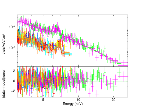
Figure 10: The XMM-Newton and NuSTAR spectra and residuals of CJ2056 fit with tbabs*(mkcflow+gauss) with $\chi_{\nu}^{2}=0.98$ for 628 degrees of freedom. The 2019 XMM-Newton observation (obsID = 0842570101) is presented in the 0.3 - 10 keV band with MOS1 in blue, MOS2 in yellow, and pn in black. Similarly, 2022 XMM-Newton observation (obsID = 0902500101) is presented in the 0.3 - 10 keV band with MOS1 in cyan, MOS2 in orange, and pn in red. The NuSTAR observation is presented in the 3-30 keV band, with FPMA in black and FPMB in red.

In nmCVs, X-ray photons are emitted from a boundary layer between the accretion disk and the WD surface. An absorbed plasma cooling model generally describes thermal X-ray emission from the shock-heated boundary layer (e.g., mkcflow). The maximum temperature ($kT_{\rm max}$) in the mkcflow model can be attributed to the shock temperature, $T_{s}$, in the boundary layer. Assuming the gravitational potential energy is converted to heat in the strong shock regime at the inner accretion disk spinning at the Keplerian velocity, the maximum temperature of the disk is given by $kT_{\rm max}=\frac{3}{16}\mu m_{\rm H}\frac{GM}{R}$ where $\mu$ is the mean molecular weight, $m_{\rm H}$ is the mass of a hydrogen atom and $R$ is the WD radius (2002apa..book.....F). More specifically, Yu2018 derived an empirical relation $kT_{\rm max}=\frac{3}{16}\alpha\mu m_{\rm H}\frac{GM}{R}$, where $\alpha$ was fit to $0.646\pm 0.069$, based on the maximum plasma temperature and known WD mass data of 11 nmCVs.

Following Yu2018, we fit an absorbed cooling flow model with a Gaussian line component to account for the neutral Fe emission line at 6.4 keV. Our spectral model, tbabs*(mkcflow+gauss), fits the XMM-Newton and NuSTAR data well, yielding $kT_{\rm max}=16.2_{-1.8}^{+1.9}$ keV, as shown in Table 6. We exclude the APEC component used in Oliveira since its contribution to the 3 - 30 keV spectra is negligible due to the low temperature ($kT=0.79$ keV). To account for the difference in flux between the NuSTAR observation and the other spectra, we fit the normalizations of mkcflow and the Gaussian component separately. As the remaining parameters only depend on fundamental properties of the WD (such as mass), which do not change with flux variations due to increased mass flow and accretion, we fit them jointly across all observations. By considering the uncertainties associated with $kT_{\rm max}$ and $\alpha$, we determined the WD mass to be $M=(0.84\rm{-}1.03)\;M_{\odot}$. The normalization of the mkcflow yields the total mass accretion rates of $\dot{M}=(3.4\pm 0.3)\times 10^{14},\;(2.6\pm 0.3)\times 10^{14}\;\rm{and}\;17.6_{-2.1}^{+2.5}\times 10^{14}$ g s${}^{-1}$ for the 2019 XMM-Newton, 2022 XMM-Newton and 2022 NuSTAR observations, respectively.

Table 6: The nmCV model fit to the X-ray spectra

Parameter	MKCFLOW
$N^{(i)}_{H}(10^{20}\rm{cm}^{-2})^{a}\;*$	4.2
$Z^{b}(Z_{\odot})$	$0.50_{-0.10}^{+0.12}$
$kT_{\rm max}$ (keV)	$16.3_{-1.9}^{+1.8}$
$EW^{c}_{\rm line}$ (eV)	$12_{-12}^{+37}$
$EW^{d}_{\rm line}$ (eV)	$138_{-65}^{+70}$
$F_{X}(10^{-12}$ ergs s${}^{-1}$ cm${}^{-2}$)${}^{e}$	6.61
$F_{X}(10^{-13}$ ergs s${}^{-1}$ cm${}^{-2}$)${}^{f}$	35.1
$\chi^{2}_{\nu}$ (dof)	0.98 (628)

All errors shown are $90\%$ confidence intervals.
${}^{a}$ The ISM hydrogen column density is associated with tbabs, which all the models are multiplied by.
${}^{b}$ Abundance relative to solar.
${}^{c}$ The equivalent width of the Gaussian component with $E=6.4$ keV and $\sigma=0.01$ keV for the both XMM-Newton datasets.
${}^{d}$ The equivalent width of the Gaussian component with $E=6.4$ keV and $\sigma=0.01$ keV for the NuSTAR data.
${}^{e}$ 3 – 10 keV flux of the XMM-Newton 2019 data.
${}^{f}$ 3 – 10 keV flux of the NuSTAR 2021 data.
${}^{*}$ The parameter is frozen.