Learning to Drive via Asymmetric Self-Play

Abstract

Large-scale data is crucial for learning realistic and capable driving policies. However, it can be impractical to rely on scaling datasets with real data alone. The majority of driving data is uninteresting, and deliberately collecting new long-tail scenarios is expensive and unsafe. We propose asymmetric self-play to scale beyond real data with additional challenging, solvable, and realistic synthetic scenarios. Our approach pairs a teacher that learns to generate scenarios it can solve but the student cannot, with a student that learns to solve them. When applied to traffic simulation, we learn realistic policies with significantly fewer collisions in both nominal and long-tail scenarios. Our policies further zero-shot transfer to generate training data for end-to-end autonomy, significantly outperforming state-of-the-art adversarial approaches, or using real data alone. For more information, visit waabi.ai/selfplay.

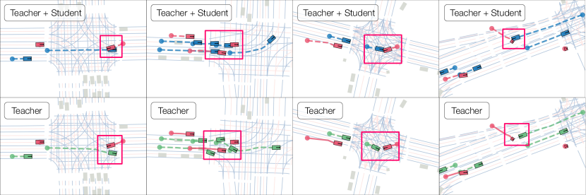
Figure 1: Asymmetric Self-Play. The teacher (red, green) learns to generate realistic scenarios where the student (blue) makes a mistake (top) while demonstrating a solution itself (bottom). The two are jointly trained to continually solve more scenarios.

1 Introduction

We are interested in developing policies that drive realistically like a human, reason about complex interactions, and handle safety-critical scenarios. While previous methods have demonstrated improved performance by applying supervised learning with gradually increasing dataset sizes, such an approach has several limitations. Collecting driving datasets at scale is extremely expensive, requiring fleets of vehicles deployed for long stretches of time. Furthermore, a central challenge of self-driving is handling rare edge cases safely, while the majority of nominal driving data is repetitive and contains little learning signal. Upsampling existing curated scenarios may help with data imbalance, but is ultimately limited by the existing collected set of logs. Yet purposefully inducing additional safety-critical scenarios in the real-world for data collection is too dangerous of a solution at scale. How can we continue to scale training data without relying solely on real-world collection?

One approach is to have policies explore novel states by leveraging closed-loop simulation and methods like reinforcement learning. However, since other actors in simulation typically exhibit nominal behavior, the resulting simulations can still be repetitive and unchallenging. Likewise, leveraging a self-play approach where a policy interacts with itself in multiagent simulation can suffer from the same issue if the policy converges to nominal and cooperative behavior. One can leverage human prior knowledge and design additional synthetic scenarios targeting particularly difficult interactions like cut-ins, but scaling the diversity of these scenarios can be difficult even with procedural generation approaches. The realism of the scenarios may also be lacking since actor behaviors are often scripted and hand-specified, which can lead to a sim-to-real gap in policies trained on these scenarios. Alternatively, adversarial optimization can be used to find trajectories that result in collision scenarios in an automated fashion. To ensure the usefulness of these scenarios for training, various solvability regularization approaches can be used (e.g. ensure the adversary doesn’t collide with the pre-recorded trajectory, or ensure a kinematically feasible solution exists). Nevertheless, scenarios can still easily end up being too easy or too difficult for the learning policy, depending on the design of such terms.

To address these shortcomings, we propose an asymmetric self-play mechanism in which challenging, solvable, and realistic scenarios naturally emerge from interactions between policies with differing objectives. We introduce the notion of a teacher and student policy (also referred to as Alice and Bob respectively in the literature), where the teacher aims to generate scenarios that the student cannot solve but the teacher itself can. This produces challenging training scenarios for the student as opposed to repeatedly training on nominal data where the learning signal is weak. Because the teacher and student improve together, novel scenarios that continue to be difficult for the student can be proposed by the teacher over the entire course of training, leading to a natural curriculum of increasingly difficult scenarios, similar to how humans learn. Finally, both policies are regularized to stay close to the data distribution to maintain realism and prevent policy collapse.

Our experiments show learning to drive via asymmetric self-play results in more realistic and robust policies. When applied to the multiagent traffic simulation problem setting, we learn actor policies with significantly reduced collision rates in both nominal scenarios and held out out-of-distribution scenarios, while still maintaining other realism metrics. We further show that these policies can zero-shot transfer to generate scenarios for new, unseen policies. This allows us to first efficiently train privileged traffic agents with self-play at scale using lightweight state simulation, before deploying these agents to interact with an end-to-end autonomy policy using high-fidelity sensor simulation. Our experiments show that training autonomy on the resulting dataset leads to far higher goal success rates and lower collision rates compared to alternatives like adversarial approaches or using real data alone.

2 Related Work

Learning to drive:

Pioneered in [55], numerous works have explored learning to drive for applications in autonomous driving [10, 18, 4, 34, 15, 84, 29, 9] and traffic simulation [5, 68, 33, 69, 85, 54, 62, 87, 67]. A popular approach is open-loop behavior cloning (BC), which reduces learning to drive to a supervised learning problem. However, BC suffers from compounding errors from distribution shift in closed-loop execution [58] and a variety of techniques have been proposed to address this problem, including data augmentation [4, 41], regularization based on prior knowledge [68, 85, 12], uncertainty-based regularization [31], inference-time search [82, 89], etc. Another approach is to train the driving policy in closed-loop with closed-loop imitation learning [68, 33, 61, 41, 69, 8], reinforcement learning [84, 85, 75, 7, 38, 90, 53], or a combination of the two [43, 85, 29]. Here, the driving policy is exposed to and learns from states induced by the consequences of its actions, thereby minimizing distribution shift. Despite these algorithmic, model, and data-scale improvements, learning-based policies still exhibit higher-than-human failure rates [27, 29], especially in highly-interactive scenarios [84]. As an orthogonal approach to learning better driving policies, in this work, we explore improvements in the training data composition and curriculum by automatically generating challenging scenarios, demonstrating its efficacy in both autonomous driving and traffic simulation.

Challenging scenarios:

Learning to handle long-tail situations from data is difficult when the majority of real-world driving data is uneventful with little learning signal. One can up-sample challenging examples from a large set of real world logs [81, 23, 60, 11], but this limits us to a fixed set of existing logs, and collecting more at scale (especially safety-critical ones) can be expensive and unsafe. Hand-designed synthetic scenarios [79, 47, 72, 24, 84] that expose the driving policy to challenging interactions can be used, but it is tedious to create realistic scenarios in this way and scaling these approaches to cover the diversity of the real world is impractical. Adversarial methods can automatically discover challenging scenarios by optimizing a fixed objective for difficulty using gradient-based optimization [28, 16, 57], Bayesian optimization [1, 78, 74], tree search [26, 36], evolutionary algorithms [35], rare-event simulation [51, 50, 64], reinforcement learning [19, 77, 17, 86, 13, 22], or retrieval augmented generation [21]. To ensure that the adversarial scenarios are useful for training, various constraints are added to encourage solvability and realism [57, 28, 78]. Unlike adversarial approaches which typically attack a fixed policy, our self-play approach allows the teacher and student to continually update and improve. Likewise, our solvability objective directly considers the current student policy rather than surrogates like the logged trajectory [78] or the result of a separate optimization process [57, 28], resulting in more relevant scenarios for training.

Self-play:

Self-play training is a popular approach to learning policies in increasingly complex and diverse environments by having them interact among copies of themselves, with recent high-profile successes in Go [63], StarCraft [76], Dota 2 [6], Diplomacy [3], etc. In the context of self-driving, [70] learns RL policies in multiagent merge traffic by having them interact in scenarios with simple rules-based agents [71] initially and then increasingly capable past copies of themselves. More generally, rules-based agents can be omitted and standard multiagent reinforcement learning (MARL) approaches can be used [90]. However, since the RL policies share a common objective, the training scenarios become increasingly uneventful and repetitive for learning as the policies converge in capabilities and learn to cooperate. In contrast, we propose to use an asymmetric self-play mechanism [66, 65, 52, 25] where a teacher (Alice) learns to propose challenging but self-solvable scenarios, and a student (Bob) learns to solve them. Whereas asymmetric self-play was first proposed for goal-discovery in RL, we use asymmetric self-play to scale our training data beyond what’s available from the real world and learn increasingly realistic and robust driving policies. To this end, we also augment the teacher’s objective to propose scenarios that are realistic as well.

3 Asymmetric Self-play for Driving

3.1 Problem Formulation

We begin by introducing the multiagent traffic modeling formulation. A traffic scenario over $T$ timesteps consists of a high definition (HD) map ${\bm{m}}$, the joint states ${\bm{s}}_{1:T}$ for $N$ actors over $T$ timesteps, and the corresponding actions ${\bm{a}}_{1:T-1}$. We use $s^{i}_{t}$ to denote the $i$-th actor’s state at time $t$, which consists of its position, heading, velocity, bounding box, and class in 2D bird’s eye view. Likewise, we use $a^{i}_{t}$ to denote the $i$-th actor’s action at time $t$, which consists of its acceleration and steering angle. Given the HD map ${\bm{m}}$ and initial states ${\bm{s}}_{1}$, we model the distribution over possible rollouts as:

$$p({\bm{s}}_{2:T},{\bm{a}}_{1:T-1}|{\bm{s}}_{1},{\bm{m}})=\prod_{t=1}^{T-1}\pi({\bm{a}}_{t}|{\bm{s}}_{\leq t},{\bm{m}})p({\bm{s}}_{t+1}|{\bm{s}}_{t},{\bm{a}}_{t})$$ (1)

where $\pi$ is a multiagent policy controlling all actors jointly and $p({\bm{s}}_{t+1}|{\bm{s}}_{t},{\bm{a}}_{t})$ is the state transition dynamics, which we model with a kinematic bicycle model [37] on a per-actor basis.

3.2 Asymmetric Self-Play Learning

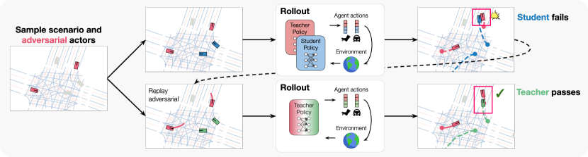
Figure 2: Method Overview. We sample an initial scene and designate adversarial actors at random. The teacher must control adversarial actors such that the student fails, but itself passes. Adversarial actions are replayed to keep the scenario the same.

Toward our goal of automatically generating challenging, solvable, and realistic scenarios for learning to drive, we design an asymmetric self-play mechanism where a teacher policy learns to propose scenarios that it can pass but a student policy fails. During training, the teacher will either control all actors in the scene or interact with a subset of student-controlled actors. When the teacher interacts with the student, it aims to cause student-controlled actors to collide; and when the teacher controls all actors, it aims to demonstrate a collision-free solution instead. The student can then improve their driving by learning to avoid collisions in the proposed scenarios. As the two are jointly trained, the teacher continually adapts their proposals to the student’s capabilities throughout learning.

Concretely, let $\pi_{T}$ and $\pi_{S}$ be the multiagent teacher and student policies respectively. A scene can be entirely controlled by the teacher by only sampling actions from $\pi_{T}$ (Eq. 1). However, it is also possible for the two policies to interact by controlling different actors within the same scene. If we partition $N$ actors into two sets ${\mathcal{T}}$ and ${\mathcal{S}}$, then the two policies $\pi_{T}$ and $\pi_{S}$ can come together as $\pi_{TS}$ to jointly control the scene,

$$\pi_{TS}(a_{t}^{i}|{\bm{s}}_{\leq t},{\bm{m}})=\begin{cases}\pi_{T}(a_{t}^{i}|{\bm{s}}_{\leq t},{\bm{m}})&\textrm{if }i\in{\mathcal{T}}\\ \pi_{S}(a_{t}^{i}|{\bm{s}}_{\leq t},{\bm{m}})&\textrm{if }i\in{\mathcal{S}}\end{cases}$$ (2)

and $\pi_{TS}({\bm{a}}_{t}|{\bm{s}}_{\leq t},{\bm{m}})=\prod_{i=1}^{N}\pi_{TS}(a_{t}^{i}|{\bm{s}}_{\leq t},{\bm{m}})$.

The teacher’s goal is to generate challenging, solvable, and realistic scenarios, so we define its objective as:

$$R_{T}({\bm{s}}_{1},{\bm{m}})=\underbrace{C(\pi_{TS},{\mathcal{S}})}_{\text{Challenging}}-\underbrace{C(\pi_{T},N)}_{\text{Solvable}}+\beta\underbrace{(I_{\text{data}}(\pi_{T})+I_{\text{data}}(\pi_{TS}))}_{\text{Realistic}}$$ (3)

where

$$C(\pi,{\mathcal{A}})=\mathbb{E}_{\pi|{\bm{s}}_{1},{\bm{m}}}\left[\sum_{i\in{\mathcal{A}}}c_{i}({\bm{s}}_{\leq T})\right]$$ (4)

$$I_{\text{data}}(\pi)=\mathbb{E}_{\pi|{\bm{s}}_{1},{\bm{m}}}\left[-\log p_{\text{data}}({\bm{s}}_{\leq T}|{\bm{m}})\right]$$ (5)

Here $c_{i}({\bm{s}})$ is an indicator function that equals 1 if actor $i$ fails (collides) and 0 otherwise. The first term $C(\pi_{TS},{\mathcal{S}})$ thus encourages the teacher to generate challenging scenarios where student-controlled actors fail. The second term $-C(\pi_{T},N)$ encourages the teacher $\pi_{T}$ to generate solvable scenarios where it can demonstrate a collision-free rollout when controlling all $N$ actors. The final term $\beta(I_{\text{data}}(\pi_{T})+I_{\text{data}}(\pi_{TS}))$ encourages the teacher to generate realistic scenarios (when the teacher controls all actors and when the teacher interacts with the student respectively), where $p_{\text{data}}$ is the data distribution and $\beta$ is a hyperparameter controlling the regularization strength.

Conversely, the student’s objective is to control its actors to avoid failures and behave realistically when interacting with the teacher.

$$R_{S}({\bm{s}}_{1},{\bm{m}})=-C(\pi_{TS},{\mathcal{S}})+\beta I_{\text{data}}(\pi_{TS})$$ (6)

Our learning framework is inspired by and resembles single-agent asymmetric self-play [52, 66] where the teacher searches for goal states that the student cannot reach. In our multiagent setting, the notion of a reachable state is instead replaced with the notion of a solvable scenario, which depends on interaction between the teacher and student. Over the course of training, the teacher and student learn together to generate a curriculum until an equilibrium is reached.

3.3 Theoretical Analysis

We now prove that for universal policies, our asymmetric self-play objective trains the student to pass all scenarios that have a reasonably realistic solution.

Definition 1

A policy $\pi_{Y}$ is $\alpha$-$\beta$-optimal if $\forall\pi_{X}$ where $I_{\text{data}}(\pi_{XY})>\alpha$ and $C(\pi_{X},N)=0$,

$$\left(C(\pi_{XY},{\mathcal{S}})>0\right)\iff\left(I_{\text{data}}(\pi_{X})<I_{\text{data}}(\pi_{XY})-\frac{1}{\beta}\right)$$ (7)

Intuitively, an $\alpha$-$\beta$-optimal policy will only fail an $\alpha$-realistic solvable scenario (as demonstrated by $C(\pi_{X},N)=0$) if the log likelihood of all possible solutions is at least $1/\beta$ lower than the log likelihood of the failure under the data distribution, where $\beta>0$ controls the realism regularization strength and is arbitrarily set.

Lemma 1

If $\pi_{T}$ and $\pi_{S}$ are in equilibrium ($\pi_{T}$ cannot improve without changing $\pi_{S}$ and vice versa), then $R_{T}\leq 2\beta I_{\text{data}}(\pi_{TS})$.

Proof

Assume that $R_{T}>2\beta I_{\text{data}}(\pi_{TS})$. Then it follows

$$-C(\pi_{T},N)+C(\pi_{TS},{\mathcal{S}})+\beta(I_{\text{data}}(\pi_{T})+I_{\text{data}}(\pi_{TS}))>2\beta I_{\text{data}}(\pi_{TS})$$ (8)

$$-C(\pi_{T},N)+\beta I_{\text{data}}(\pi_{T})>-C(\pi_{TS},{\mathcal{S}})+\beta I_{\text{data}}(\pi_{TS})$$ (9)

However, Eq. 9 shows that then $\pi_{S}$ can improve its return (Eq. 6) by simply copying $\pi_{T}$, which contradicts the equilibrium assumption. ∎

Theorem 3.1

If $\pi_{T}$ and $\pi_{S}$ are in equilibrium, then $\pi_{S}$ is $\alpha$-$\beta$-optimal, where $\alpha=I_{\text{data}}(\pi_{TS})+\frac{1}{2\beta}$.

Proof

Assume that $\pi_{S}$ is not optimal. Then there must exist a $\pi_{X}$ where $I_{\text{data}}(\pi_{XS})>\alpha$ and $C(\pi_{X},N)=0$ for which

$$\left(C(\pi_{XS},{\mathcal{S}})>0\right)\land\left(I_{\text{data}}(\pi_{X})>I_{\text{data}}(\pi_{XS})-\frac{1}{\beta}\right).$$ (10)

Then it follows:

$$C(\pi_{XS},{\mathcal{S}})+\beta I_{\text{data}}(\pi_{X}) >C(\pi_{X},N)+\beta I_{\text{data}}(\pi_{XS})-1$$ (11)

$$R_{X} >2\beta I_{\text{data}}(\pi_{XS})-1$$ (12)

$$R_{X} >R_{T}$$ (13)

where Eq. 11 uses the fact that $C(\pi_{X},N)=0$, Eq. 12 comes from adding $\beta\left(I_{\text{data}}(\pi_{XS})+I_{\text{data}}(\pi_{X})\right)$ to both sides, and Eq. 13 comes from substituting in $I_{\text{data}}(\pi_{XS})>\alpha$ and applying Lemma 1. However, this shows that $\pi_{T}$ can improve by copying $\pi_{X}$, contradicting the equilibrium assumption. ∎

Thus we see under the proposed asymmetric self-play objective, a student in equilibrium with the teacher should solve any reasonably realistic solution.

3.4 Ensuring Fair-play

While Eq. 3 encourages teacher-solvable scenarios, the teacher has an unfair advantage as it can coordinate all actors. For example, the teacher may try to identify student-controlled actors and propose more difficult (and potentially unsolvable) scenarios only for the student. This impedes the student’s ability to learn and thus motivates additional restrictions on the teacher.

3-player formulation:

To address unfair coordination, we can divide the teacher into two sub-policies, adversary and demonstrator. When $\pi_{T}$ is used to control all $N$ actors, the adversary sub-policy controls actors in ${\mathcal{T}}$ and the demonstrator sub-policy controls actors in ${\mathcal{S}}$. Thus any coordination the demonstrator may try with the adversary can in principle be learned by the student, as their architectures are now identical.

Replay actions:

Note that the teacher’s reward in Eq. 3 is a function of a pair of rollouts sampled from $\pi_{T},\pi_{TS}$ using identical initial conditions ${\bm{s}}_{1},{\bm{m}}$. We can replay states for actors in ${\mathcal{T}}$ in one simulation from the pair. Let $\bar{{\bm{a}}}_{\leq T}$ be actions sampled from $\pi_{TS}$. Then when rolling out $\pi_{T}$, we instead use the modified policy

$$\hat{\pi}_{T}(a_{t}^{i}|{\bm{s}}_{\leq t},{\bm{m}})=\begin{cases}\delta(a_{t}^{i}-\bar{a}^{i}_{t})&\textrm{if }i\in{\mathcal{T}}\\ \pi_{T}(a_{t}^{i}|{\bm{s}}_{\leq t},{\bm{m}})&\textrm{otherwise }\end{cases}$$ (14)

where $\delta$ is the Dirac-$\delta$ function. This prevents the teacher from treating itself differently and enforces it to solve the exact same scenario subjected to the student. While the equation above is illustrative for when actors in $\pi_{T}$ is replayed, during training, we randomly select whether $\pi_{T}$ or $\pi_{TS}$ is replayed.

3.5 Implementation

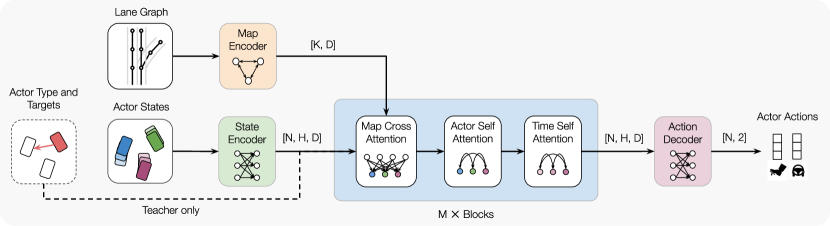
Figure 3: Policy Architecture. We encode $K$ lane graph nodes and state history for $N$ actors over $H$ history timesteps into $D$-dimensional features. A transformer backbone with $M$ blocks uses factorized attention to extract features before decoding them into actor steering and acceleration. The teacher policy additionally encodes actor type (if an actor is in ${\mathcal{T}}$) and target information; the student does not observe this information.

Neural Network Architecture:

We implement our policy network with a viewpoint-invariant transformer [73]. Given a lane graph ${\bm{m}}$ with $K$ nodes, we first use a viewpoint-invariant map encoder [20] to extract a set of lane graph node features,

$$\{{\bm{f}}_{k}\}_{k=1}^{K}=\mathrm{MapEncoder}({\bm{m}})$$ (15)

For each actor $i$, our state encoder uses a multi-layer perceptron (MLP) to extract features for its past state $s_{t-H}^{i},\ldots,s_{t}^{i}$ over the past horizon $H\geq 1$,

$${\bm{h}}_{t^{\prime}}^{i}=\mathrm{StateEncoder}(\varphi_{t\rightarrow t^{\prime}}^{i}\oplus[v_{t^{\prime}}^{i},\ell^{i},w^{i}]),\quad t^{\prime}=t-H+1,\ldots,t$$ (16)

where $\oplus$ is the concatenation operator, $v^{i}_{t^{\prime}},\ell^{i},w^{i}$ is the actor’s velocity, length, and width, and $\varphi_{t\rightarrow t}^{i}$ is the PairPose relative positional features between the actor’s position at the current time $t$ and past time $t^{\prime}$; i.e., $g_{i\rightarrow j}^{a}$ in [20, Eq. 1]. Each actor feature ${\bm{h}}_{t^{\prime}}^{i}$ encodes the $i$-th actor’s state at $t^{\prime}$ in its local coordinate frame at $t$, therefore preserving viewpoint-invariance.

Next, we use a stack of interleaving actor-to-map, actor-to-actor, and actor-to-time transformer layers [49] to efficiently model actor and lane graph interactions. Our actor-to-time layer uses standard self-attention, with sinusoidal positional encoding to break the symmetry across time. To model actor-to-actor interactions in a viewpoint-invariant manner, we extend standard self-attention to use relative positional encodings between actors [92, 88]. For the $i$-th actor at time $t^{\prime}$, we compute attention with key ${\bm{k}}_{i}$, queries $\{{\bm{q}}_{i,j}\}_{j=1}^{N}$, and values $\{{\bm{v}}_{i,j}\}_{j=1}^{N}$,

$${\bm{k}}_{i}={\bm{h}}_{t^{\prime}}^{i},\quad{\bm{q}}_{i,j}={\bm{v}}_{i,j}={\bm{h}}_{t^{\prime}}^{j}+\mathrm{MLP}(\varphi_{t^{\prime}}^{i\rightarrow j})$$ (17)

where $\varphi_{t^{\prime}}^{i\rightarrow j}$ is the PairPose features between actors $i$ and $j$ at time $t^{\prime}$.

We use the same attention mechanism in our actor-to-map layer with two modifications for efficiency: 1) we use actor-to-map only for the current time $t$ and 2) we limit its queries and values to the actor’s $k$ nearest lane graph nodes.

Finally, our action decoder uses an MLP to deterministically predict each actor’s steering and acceleration from its features ${\bm{h}}_{t}^{i}$ at the current time $t$ after $M$ blocks of transformer layers.

$${\bm{a}}_{t}^{i}=\mathrm{ActionDecoder}({\bm{h}}_{t}^{i})$$ (18)

The policy can then be unrolled in the environment in a sliding window fashion.

Optimization:

We describe how to optimize Eqs. 3 and 6 in practice. During training, we randomly assign agents into ${\mathcal{T}}$. For ease of optimization, we 1) relax the discrete indicator function $c_{i}({\bm{s}})$ to a differentiable collision loss, 2) assign a specific target actor for each actor in ${\mathcal{T}}$ for which the collision loss is active, and 3) apply an additional distance loss to encourage each adversarial actor towards its target. To encode the information that actor $i$ targets actor $j$, we have

$${\bm{h}}_{t}^{i}\leftarrow{\bm{h}}_{t}^{i}+\mathrm{MLP}({\bm{e}}\oplus\varphi_{t}^{i\rightarrow j})$$ (19)

where ${\bm{e}}$ is a learnable embedding to indicate the actor is in ${\mathcal{T}}$ and the PairPose features provide positional information on the target. In the 3-player formulation, only the adversarial sub-policy has access to this information. Finally, as our relaxed reward is differentiable, we can use backpropagation through time to directly optimize the learning objective.

4 Experiments

4.1 Realistic Traffic Simulation

Datasets:

We use three different datasets to evaluate our model’s performance. Argoverse2 Motion [81] is a collection of 250k urban scenarios curated for challenging multiagent-interactions. Agents are given 5s of history before unrolling for 6s. Our policy observes all actors but only controls focal and scored agents while the remaining actors are replayed due to noisy or incomplete annotations.

Next, Highway is a collection of over 1000 highway logs collected over various locations including on-ramps, off-ramps, forks, merges, and curved roads. Agents are given 3s of history before unrolling for 10s. As Highway consists of high-quality human labels, all actors are controlled.

Finally, Safety is a collection of over 100 hand-designed safety-critical highway scenarios with various edge cases including aggressive actor cut-ins, lead actor hard-braking, actors stopped on shoulder, etc. These scenarios are simulated and involve actors that are scripted to induce safety-critical interactions while the actor policy controls the ego actor that is meant to be tested. As Safety scenarios are simulated and interactive to the policy being evaluated, no ground truth human demonstrations are available. We use Safety to evaluate models trained on Highway without any fine-tuning, measuring their out-of-distribution generalization to highly-interactive, safety-critical scenarios.

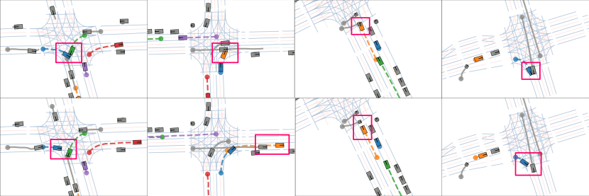
Figure 4: Qualitative Comparison. We show TrafficSim (top) and Ours (bottom) on Argoverse2. Our method learns better interaction reasoning to avoid collisions realistically. Colored actors are controlled; gray actors are replayed.

Traffic Modelling Metrics:

We use a suite of metrics to evaluate the realism of traffic simulation agents. Final displacement error (FDE) measures the L2 error between the agent’s simulated future and ground truth (GT) position at the end of the rollout. Collision percent is used to evaluate actors’ interaction reasoning, and Offroad percent evaluates actors’ map understanding. We also measure the distributional similarity of various actor features. This is done by fitting histograms to agents’ linear speed, linear acceleration, angular speed, distance to road boundary, and distance to the closest actor, before taking the Jensen-Shannon divergence (JSD) to the GT statistics. Following [48], GT statistics are computed for each actor separately, with time being considered independent. These are then averaged to form our composite JSD metric.

Baselines:

We compare our approach against the current state-of-the-art for traffic simulation. Closed-loop IL is our supervised learning baseline that is trained to regress expert states using closed-loop policy unrolling [68]. TrafficSim [68] further incorporates prior knowledge to closed-loop IL using a differentiable collision loss. For our standard symmetric self-play baseline, we adapt the multiagent RL (MARL) approach in SMARTS [90] to our setting by applying a factorized PPO loss [85] to the multiagent policy to optimize a hand-designed reward. Emb. Syn. [11] is a curation-based approach which sub-samples the dataset using a learned difficulty classifier. As [11] uses an extremely large internal dataset containing a 14k hours of driving, to adapt their approach to the datasets used in this work, we 1) directly select the snippets where the baseline IL model fails in rather than training a difficulty classifier and 2) finetune the baseline IL model on the selected snippets instead of training from scratch. KING [28] is a gradient-based adversarial approach where the adversarial objective is backpropagated through bicycle model dynamics. We adapt [28] to generate adversarial training examples with the same realism regularization term as ours (stay close to the logged trajectory) for training the base traffic policy. All baselines are adapted to use the same input/output representation, model architecture, and environment dynamics. More details can be found in the supplementary.

	Safety	Highway				Argoverse2
Model	Col.	FDE	Col.	Offroad	JSD	FDE	Col.	Offroad	JSD
Closed-loop (IL) [68]	40.41	5.70	1.88	1.43	0.460	4.95	1.02	3.14	0.436
TrafficSim (IL+Prior) [68]	26.69	5.83	0.37	1.39	0.466	5.13	0.33	3.36	0.436
SMARTS (MARL) [90]	13.65	20.2	0.99	2.97	0.501	16.3	8.12	17.2	0.528
Emb. Syn. (Curation) [11]	27.75	6.46	4.34	1.67	0.490	6.89	2.02	4.30	0.449
KING (Adversarial)  [28]	12.65	5.80	1.42	1.59	0.475	6.33	1.16	3.29	0.465
Ours	8.16	5.76	0.00	1.40	0.462	5.04	0.24	3.39	0.433

Table 1: Traffic Simulation Results. On Safety, Highway, and Argoverse2, our approach obtains the best collision rates without sacrificing other realism metrics.

Results:

Recall that models trained on Highway are evaluated on Safety without fine-tuning. Tab. 1 shows that the IL baseline consistently achieves the best reconstruction metrics but struggles with interaction reasoning, resulting in higher collision rates. By adding in prior knowledge using the differentiable collision loss, TrafficSim can reduce the collision rate with some trade-off in other realism metrics. MARL struggles the most as it is difficult to capture realistic human-like driving with a handcrafted reward alone. Curation is ineffective at our dataset scale, even for Argoverse2 which is among the largest publicly available datasets. This is potentially because Argoverse2 is already curated. KING reduces collision rate on Safety but still struggles with nominal collisions. This could be due to the fact that the realism of the adversarial trajectories is lacking, lowering their transferability. Our approach consistently achieves the best overall realism, achieving the lowest collision rates with minimal sacrifice in other metrics, and generalizes the best to the Safety set.

4.2 Zero-shot Scenario Generation for Learnable Autonomy

In Sec. 4.1, we have shown that after self-play training, the teacher has helped the student learn a more realistic and robust policy for multiagent traffic simulation. We now evaluate the teacher’s ability to zero-shot transfer to generate scenarios for new unseen policies. The ability for zero-shot transfer not only shows that the teacher policy has learned generally applicable training scenarios but also provides an efficient way to improve more expensive policies. Traffic simulation agents use low dimensional (bicycle model) states as input, so they can be efficiently trained at scale with lightweight and efficient simulation. Agents can then be deployed to interact with end-to-end autonomy policies that require additional more expensive high-fidelity sensor simulation. This allows us to generate training scenarios for the autonomy policy by simply deploying our teacher policy to target the external policy, without needing to retrain in the more expensive simulation setting.

			Safety						Highway
Autonomy	Train Data	Priv	GSR ($\uparrow$)	Col ($\downarrow$)	mTTC ($\mathrm{\Delta}$)	Prog ($\mathrm{\Delta}$)	P2E ($\mathrm{\Delta}$)	Accel ($\mathrm{\Delta}$)	Col ($\downarrow$)	mTTC ($\mathrm{\Delta}$)	Prog ($\mathrm{\Delta}$)	P2E ($\mathrm{\Delta}$)	Accel ($\mathrm{\Delta}$)
Expert		✓	90.6	0.0	5.82	232	0.17	0.85	0.0	4.15	483	0.27	0.25
Object- based	Safety	✓	80.1	0.0	5.83	236	0.35	0.91	0.0	4.28	487	0.05	0.14
	Highway		40.2	58.3	3.33	280	1.01	1.41	0.0	4.16	498	0.02	0.14
	IL [68]		45.6	59.7	3.61	277	0.90	1.39	0.0	4.17	498	0.02	0.11
	Adv. [28]		83.1	6.2	5.54	253	0.45	0.99	0.0	4.20	500	0.03	0.12
	Ours		92.6	0.0	5.77	247	0.36	0.88	0.0	4.29	482	0.09	0.18
Object- free	Safety	✓	64.2	0.0	6.14	170	0.43	1.19	0.0	4.78	297	0.80	1.08
	Highway		31.2	52.3	3.08	267	1.15	1.28	0.0	4.56	460	0.48	0.36
	IL [68]		35.8	52.3	2.99	270	1.12	1.27	0.0	4.62	462	0.45	0.35
	Adv. [28]		38.7	50.9	2.96	273	1.06	1.26	0.0	4.46	467	0.40	0.32
	Ours		64.2	0.0	6.15	169	0.52	1.23	0.0	4.67	300	0.75	1.02

Table 2: End-to-end autonomy results on Safety and Highway. $(\uparrow/\downarrow)$ denotes higher/lower is better, $(\mathrm{\Delta})$ denotes closer to expert is better. Among the unprivileged methods, we obtain the best overall performance, with emphasis on Safety.

Learnable Autonomy Systems:

To evaluate the generalizability of our approach, we consider training two distinct autonomy paradigms on datasets generated using our approach versus various baselines. Our object-based autonomy estimates actor locations with a discrete set of bounding boxes and trajectories using a joint perception and prediction backbone [44, 40, 14]. Our object-free autonomy estimates actor locations with continuous occupancy probabilities across the scene [45, 2] to be used for motion planning [32, 15, 9]. Both approaches sample trajectories in Frenet frame before costing each trajectory and selecting the min-cost trajectory [59]. Costs are computed as a linear combination of several trajectory features, where weights are learned using max margin [59, 83]. Expert demonstrations are generated using an oracle planner with privileged access to ground truth actor states and future plans. As both autonomy approaches use LiDAR input, LidarSim [46] is used for training-dataset generation and evaluation in closed-loop simulation. More details can be found in the supplementary.

Autonomy Evaluation:

We evaluate an autonomy’s nominal driving with Highway in reactive log replay, and safety-critical performance with Safety (both datasets described in Sec. 4.1). For our primary system performance and safety metrics, Goal Success Rate (GSR) measures if the ego reaches its goal without violating traffic rules or colliding, and Collision (Col) measures collisions with the ego vehicle. We use secondary metrics to measure other aspects of driving quality. Minimum Time-To-Collision (mTTC) is computed between the ego vehicle and other actors assuming constant velocity and acceleration. Progress (Prog) is the distance traveled over the scene. Plan to Execution (P2E) is the deviation between the ego plan and its executed trajectory, measuring a notion of planning consistency. Acceleration (Accel) is the average of the longitudinal and lateral acceleration, measuring discomfort. Primary metrics have a clear direction where higher/lower is better. Secondary metrics are less clear (e.g. progress should be high but not compromise safety/speed-limit, P2E should be low in general but high when encountering unexpected behaviors). Thus secondary metrics are better if they are closer to the expert.

Baselines:

Our first baseline is using Highway in reactive log replay. Next, we use Closed-loop IL and Adversarial (Sec. 4.1) to generate datasets. Finally, we report two privileged approaches: 1) the performance of the expert autonomy and 2) the performance of training directly on the Safety test set.

Results:

Tab. 2 shows that nominal driving (Highway, IL) does not contain enough exposure to edge cases for autonomy to generalize to the Safety set. Adversarial generation improves performance but is still lacking. We posit that the per-scenario optimization process reaches local optima that our approach has learned to avoid over the course of training. Similarly, our model also learns more general notions of realism, compared to the per-scenario objective of staying close to the logged trajectory. These factors are particularly pronounced for our object-free autonomy, which relies on more difficult scenarios during training but results in more conservative driving. Thus, we achieve high-quality driving performance for both Safety and Highway evaluation, closely matching the performance of the privileged approaches across both autonomy paradigms.

4.3 Ablation and Analysis

In this section, we ablate various aspects of our asymmetric self-play learning objective and model architecture using the traffic simulation setting as a test bed. We also provide additional analysis of the training dynamics of our approach.

Ablation:

		Highway			Safety
Solv. Obj.	Realism Obj.	FDE	Col.	JSD	Col.
		7.12	2.48	0.529	16.37
✓		8.16	2.33	0.536	18.62
	✓	6.75	1.75	0.513	2.14
✓	✓	5.79	0.00	0.464	8.78

Table 3: Teacher loss design.

		Highway			Safety
3-player Game	Replay Actions	FDE	Col.	JSD	Col.
		5.90	0.29	0.478	1.3
✓		6.00	0.09	0.474	12.4
	✓	6.02	0.07	0.457	12.4
✓	✓	5.79	0.00	0.464	8.78

Table 4: Teacher architecture design.

First we ask, how important is it for challenging scenarios to be solvable and realistic? We ablate the solvability and realism terms in the teacher objective in Eq. 3; Tab. 4 shows that both are necessary for the student to learn realistic and robust behavior. Without solvability, the teacher generates extremely difficult scenarios, resulting in an overly cautious student which avoids collisions on Safety but drives poorly in nominal scenarios, exhibiting unnecessary and extreme evasive maneuvers. Without any realism, scenarios become so extreme that they no longer even transfer to Safety.

Next we ask, how effective are the fair-play architectural design choices presented in Sec. 3.4? Tab. 4 shows that combining the 3-player and replay approach results in the best overall performance. Using neither of the two achieves a very low Safety collision rate at the cost of greatly increasing nominal collisions. This is because the teacher overestimates the solvability of a scenario, leading to similar outcomes as when the solvability loss term is omitted.

Adversarial Success vs. Student Performance:

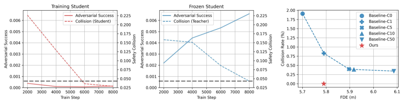
Figure 5: (Left): When the student is training, adversarial success plateaus but the student continually improves. (Center): When the student is frozen, adversarial success improves along with teacher performance. (Right): Our approach dominates the Pareto frontier obtained from naively increasing collision loss weight.

We wish to analyze the correlation between adversarial success, (the teacher’s ability to find solvable scenarios that the student fails) and the performance of the student. Fig. 5 (left) shows the teacher’s return (minus realism) and the student’s performance on Safety. Despite the teacher’s return staying flat, the student continually improves. Because the student trains with the teacher, it is difficult for the teacher to consistently outperform the student to improve its objective. Fig. 5 (right) shows the teacher’s performance when the student is frozen. In this case teacher can continually increase its return by exploiting scenarios the frozen student fails. However, there is less incentive for the teacher to increase the difficulty of the training scenarios, resulting in the teacher having worse performance compared to a continually improving student.

Pareto Frontier:

We show in Fig. 5 (right) that the improvements of our approach cannot be obtained by increasing the weight on the differentiable collision loss in TrafficSim. Our results suggest that difficult scenarios are more useful for learning robust policies while maintaining performance on nominal driving.

5 Conclusion and Limitations

We have presented an asymmetric self-play approach for learning to drive, where solvable and realistic scenarios naturally emerge from the interactions of a teacher and student policy. We have shown that the resulting student policy can power more realistic and robust traffic simulation agents across several datasets, and the teacher policy can zero-shot generalize to generating scenarios for unseen end-to-end autonomy policies without needing expensive retraining. While the results are promising, we recognize some existing limitations. Firstly, the specific type of scenarios the teacher finds is not controllable; incorporating advances in controllable traffic simulation or exploring alternative reward designs and training schemes to encourage diversity can be interesting directions to explore. Exploring alternative failure modes besides collision (e.g. off-road, unrealistic behaviors, perception failures) is another promising avenue for future work.

Learning to Drive via Asymmetric Self-Play
Supplementary Material

In this supplementary material, we present additional implementation details in Appendix 0.A, more information about baselines in Appendix 0.B, and more information about the learnable autonomy systems used in Appendix 0.C, more detailed theoretical analysis in Appendix 0.D, and additional quantitative results in Appendix 0.E and additional qualitative results in Appendix 0.F. The supplementary zip file also includes a video containing an overview and qualitative results.

Appendix 0.A Implementation Details

We first present the full algorithms used in Secs. 4.1 and 4.2 in Algorithms 1 and 2 respectively. Then we provide additional implementation details our architecture, environment, loss and training.

Overall Algorithms:

For clarity, we present the full training algorithm for the traffic modeling problem setting in Algorithm 1, and the algorithm for improving end-to-end autonomy in Algorithm 2.

Architecture:

Our transformer model uses a hidden dimensionality of 128, with 8 attention heads and a feed-forward dimensionality of 512. We use 6 transformer blocks. Our map encoder uses the same hidden dimensionality of 128. For the edge MLP in LaneGCN, the dimensionality is 64. Our action decoder is a 3 layer MLP with hidden dimensionality of 64 as well.

Environment:

Recall that the kinematic bicycle model [37] is used for environment dynamics. The state in the bicycle model state is

$$s=(x,y,\theta,v)$$ (20)

where $x,y$ is the position of the center of the rear axel, $\theta$ is the yaw, and $v$ is the velocity. The actions are

$$a=(u,\phi)$$ (21)

where $u$ is the acceleration, and $\phi$ is the steering angle. The dynamics function $\dot{s}=f(s,a)$ is then defined as

$$\dot{x} =v\cos(\theta)$$ (22)

$$\dot{y} =v\sin(\theta)$$ (23)

$$\dot{\theta} =\frac{v}{L}\tan({\phi})$$ (24)

$$\dot{v} =u$$ (25)

where $L$ is wheelbase length, i.e. the distance between the rear and front axel. We use a finite difference approach to compute the next state

$$s_{t+1}=s_{t}+f(s_{t},a_{t})\mathrm{d}t.$$ (26)

For traffic modeling, our simulation frequency is 2Hz, so $\mathrm{d}t=0.5$

Algorithm 1 Asymmetric Self-play

1:  Initialize $\pi_{T}$ and $\pi_{S}$

2:  for $i=1,\ldots,\texttt{num\_iters}$ do

3:     Sample initial state and map ${\bm{s}}_{1},{\bm{m}}$ from dataset ${\mathcal{D}}$

4:     Randomly partition all $N$ actors into ${\mathcal{T}}$ and ${\mathcal{S}}$

5:     Initialize target information $\zeta$ for actors in ${\mathcal{T}}$

6:     if Uniform(0, 1) < 0.5 then

7:        Sample ${\color[rgb]{0,0.88,0}\bm{{\bm{s}}_{\leq T},{\bm{a}}_{\leq T}}}$ using $\pi_{T}(\cdot|{\bm{s}}_{1},{\bm{m}},{\mathcal{T}},\zeta)$

8:        Sample ${\color[rgb]{0.0600000000000001,0.46,1}\bm{\widetilde{{\bm{s}}}_{\leq T},\widetilde{{\bm{a}}}_{\leq T}}}$ using $\hat{\pi}_{TS}(\cdot|{\bm{s}}_{1},{\bm{m}},{\mathcal{T}},\zeta)$, with replayed actions (Eq. 14)

9:     else

10:        Sample ${\color[rgb]{0.0600000000000001,0.46,1}\bm{\widetilde{{\bm{s}}}_{\leq T},\widetilde{{\bm{a}}}_{\leq T}}}$ using $\pi_{TS}(\cdot|{\bm{s}}_{1},{\bm{m}},{\mathcal{T}},\zeta)$

11:        Sample ${\color[rgb]{0,0.88,0}\bm{{\bm{s}}_{\leq T},{\bm{a}}_{\leq T}}}$ using $\hat{\pi}_{T}(\cdot|{\bm{s}}_{1},{\bm{m}},{\mathcal{T}},\zeta)$, with replayed actions (Eq. 14)

12:     end if

13:     Compute ${\color[rgb]{0,0.88,0}\bm{R_{T}}}$ using ${\color[rgb]{0,0.88,0}\bm{{\bm{s}}_{\leq T},{\bm{a}}_{\leq T}}}$ (Eq. 3)

14:     Compute ${\color[rgb]{0.0600000000000001,0.46,1}\bm{R_{S}}}$ using ${\color[rgb]{0.0600000000000001,0.46,1}\bm{\widetilde{{\bm{s}}}_{\leq T},\widetilde{{\bm{a}}}_{\leq T}}}$(Eq. 6)

15:     Update $\pi_{T}$ parameters with $\nabla{\color[rgb]{0,0.88,0}\bm{R_{T}}}$

16:     Update $\pi_{S}$ parameters with $\nabla{\color[rgb]{0.0600000000000001,0.46,1}\bm{R_{S}}}$

17:  end for

Loss:

As described in the main paper, our IL regularization loss is given as

$$L_{\text{IL}}=\mathbb{E}_{\pi}\left[\frac{1}{T}\sum_{t=1}^{T}D({\bm{s}}_{t},{\bm{s}}^{\text{data}}_{t})\right]$$ (27)

where $D$ is the Huber loss.

Recall that we make use a differentiable collision function as well. To compute a pairwise collision loss, vehicles are approximated with 5 circles, and the L2 distance between centroids of the closest circles of each pair of actors is used. Specifically, we have

$$\ell(s^{i},s^{j})=\min_{P\times Q}\text{relu}(r_{p}+r_{q}-d_{pq}+b)$$ (28)

where $P$ and $Q$ is the set of circles for actor $i$ and $j$ respectively, $r$ is the radius of a circle, $d_{pq}$ is the L2 distance between the centroids of two circles, $b$ is an additional safety buffer (which we set to 0.2), and $\text{relu}(x)=\max(0,x)$. The total collision loss can be computed as the average of the pairwise collision losses

$$L_{\text{Collision}}=\frac{1}{NT}\sum_{t=1}^{T}\sum_{i\neq j}\ell(s^{i}_{t},s^{j}_{t})$$ (29)

Training:

We use AdamW [42] as our optimizer. We use a linear warmup over 100 steps to an initial learning rate of 0.0001 before using a cosine decay schedule down to a learning rate of 0. For Highway, we train for 10000 steps, and for Argoverse2 we train for 30000 steps. We use a batch size of 32—note that because are using a closed-loop learning approach, a single example corresponds to a full rollout (20 steps for Highway, 12 steps for Argoverse2).

Algorithm 2 Zero-shot Scenario Generation for Learnable Autonomy

1:  Initialize learnable autonomy $\pi_{A}$

2:  Obtain expert privileged autonomy policy $\pi_{E}$

3:  Obtain pre-trained teacher policy $\pi_{T}$ from Algorithm 1

4:  Initialize ${\mathcal{D}}_{\text{Autonomy}}=\emptyset$

5:  for $i=1,\ldots,\texttt{desired\_size}$ do

6:     Sample initial state and map ${\bm{s}}_{1},{\bm{m}}$ from dataset ${\mathcal{D}}$

7:     Randomly partition all $N$ actors into ${\mathcal{T}}$ and ${\mathcal{S}}$, ensuring ego actor is in ${\mathcal{S}}$

8:     Initialize target information $\zeta$ for actors in ${\mathcal{T}}$, ensuring ego actor is targeted

9:     Sample ${\bm{s}}_{\leq T},{\bm{a}}_{\leq T}$ using $\pi_{T}(\cdot|{\bm{s}}_{1},{\bm{m}},{\mathcal{T}},\zeta)$, with $\pi_{E}$ controlling the ego actor

10:     Obtain sensor data $X_{\leq T}=\text{LidarSim}({\bm{s}}_{\leq T},{\bm{a}}_{\leq T})$ from state data

11:     Add to dataset ${\mathcal{D}}_{\text{Autonomy}}={\mathcal{D}}_{\text{Autonomy}}\cup\{(X_{\leq T},{\bm{s}}_{\leq T})\}$

12:  end for

13:  for $i=1,\ldots,\texttt{num\_iters}$ do

14:     Sample $(X_{\leq T},{\bm{s}}_{\leq T})\sim{\mathcal{D}}_{\text{Autonomy}}$

15:     Compute max margin loss $J$ using $\pi_{A},\pi_{E},X_{\leq T},{\bm{s}}_{\leq T}$ (Eq. 38)

16:     Update $\pi_{A}$ using $\nabla J$

17:  end for

Appendix 0.B Baselines

In this section, we provide more details on the baselines used in Secs. 4.1 and 4.2. All baselines are adapted to use the same architecture, input/output representation, and environment dynamics model as our approach when applicable. We now present specific details for each individual baseline.

Closed-loop IL [68]:

This baseline is representative of state of the art supervised learning approaches to traffic modeling. We use the same IL loss described in Eq. 27.

TrafficSim [68]:

This baseline further incorporates prior knowledge to closed-loop IL. We use the same collision loss as described in Eq. 29.

SMARTS [90]:

This baseline is representatitive of multiagent reinforcement learning (MARL), or standard self-play approaches. Our reward consists of collision, off-road, route progress and route completion. For this baseline, collision is computed exactly by looking at bounding box overlap between actors as a differentiable relaxation is no longer needed when using RL. Off-road is similarly computed by seeing if an actors’ bounding box leaves the drivable area. Both collision and off-road are sparse, and return $-1$. Actors that encounter collision or off-road events have their episode terminated. Since we initialize scenarios from logs, we reconstruct a route for each actor using their ground truth future trajectory. Specifically, the route is a sequence of lane graph nodes that are closest to the trajectory. Route progress is then computed as

$$R_{\text{progress}}(s_{t},s_{t-1})=\max(p_{t}-p_{t-1},\text{speed limit})\exp(-0.2c_{t})$$ (30)

where $p_{t}$ is the normalized distance along the route at time $t$, and $c_{t}$ is the cross track distance away from the route, to penalize route deviation. Route completion gives a reward for when an actor reaches past 95% of the distance along the route, and also terminates their episode. The total reward we use is then

$$R_{\text{total}}=R_{\text{collision}}+R_{\text{off-road}}+0.05R_{\text{progress}}+0.01$$ (31)

where we have a small reward of $0.01$ for continuing to survive without having the episode terminated. To improve training efficiency, when one actor has their episode terminated, they are simply removed from the scene, and the remaining actors continue simulation. This prevents extremely short episodes in the beginning of training.

Note that our total reward is defined on a per-actor basis. Following [85], we use a per-actor factorized PPO loss. The value model is trained using per-agent value targets, which are computed with per-agent rewards $R^{(i)}_{t}=R^{(i)}({\bm{s}}_{t},a_{t}^{(i)})$

$${\mathcal{L}}^{\text{value}} =\sum_{i}^{N}(\hat{V}^{(i)}-V^{(i)})^{2}$$ (32)

$$V^{(i)} =\sum_{t=0}^{T}\gamma^{t}R^{(i)}_{t}$$ (33)

The per-actor GAE is computed as

$$A^{(i)}=\text{GAE}(R^{(i)}_{0},\dots,R^{(i)}_{T-1},\hat{V}^{(i)}({\bm{s}}_{T})).$$ (34)

The PPO policy loss is then computed a sum over a per-actor PPO loss,

$${\mathcal{L}}^{\text{policy}}=\sum_{i=1}^{N}\min(r^{(i)}A^{(i)},\text{clip}(r^{(i)},1-\epsilon,1+\epsilon)A^{(i)})$$ (35)

and the overall loss is a combination of the policy and value loss

$${\mathcal{L}}^{\text{RL}}={\mathcal{L}}^{\text{policy}}+{\mathcal{L}}^{\text{value}}.$$ (36)

Finally, unlike other baselines, our MARL baseline uses a discrete action space outperforms a continuous action space. Specifically, our action space is the cross product of 5 lateral buckets and 10 longitudinal buckets. We found that by increasing simulation frequency from 2hz to 10hz, this discrete action space performs better than simply using continuous actions.

Emb. Syn. [11]:

This baseline is representative of curation and upsampling approaches. Originally, [11] uses a 14000-hour internal driving dataset, and train a difficulty classifier to upsampling difficult scenarios. However, in our case, the dataset sizes are more limited, e.g. Argoverse Motion is among the largest public driving datasets, and contains around 700 hours. Thus, to adapt curation approaches to these dataset scales, rather than training a difficulty classifier, we simply find scenarios that the baseline Closed-loop IL approach fails and create our curated set based on that. Then, we additionally fine tune the same baseline model on the curated set of failure cases. Failure in this case is simply defined as any scenario where at least actor is colliding with another actor.

KING [28]:

This baseline is representative of adversarial optimization based approaches. [28] exploits the differentiability of the bicycle model to directly do gradient-based optimization of an adversarial objective. In our implementation, we use the same adversarial actor and target selection as our approach. The adversarial objective is defined as

$$L_{adv}=-10L_{\text{Collision}}+L_{\text{Distance}}+L_{\text{IL}}$$ (37)

where the collision and IL loss are those defined in Eqs. 27 and 29, and the distance loss is simply the L2 distance to the targeted actor. Adversarial scenarios can then be found by optimizing this objective, with the constraint that for scenarios where a collision is found, a kinematically feasible solution can also be found. We find the solution by simply optimizing $L_{\text{Collision}}$ for the non-adversarial actors.

To use KING to improve actor models, we train using the same losses as TrafficSim, and include an equal mix of nominal and KING-discovered scenarios. Specifically, the adversarial optimization is run online against the current learning policy. To use KING to improve autonomy, we perform adversarial optimization against the expert autonomy to create a dataset, and train on the resulting scenarios. All scenarios are used regardless if a collision was actually found, since for many cases even if no collision is found, the expert autonomy is forced to perform an evase maneuver, which serves as good training data.

Appendix 0.C Learnable Autonomy

In this section, we provide additional details on the learnable autonomy systems used in Sec. 4.2.

Object-based Autonomy:

The most common structured autonomy paradigm consists of chaining perception, prediction, and motion planning. Following [14], we use a joint perception and prediction transformer backbone. Firstly, LiDAR features are extracted by using a PointNet [56] for points residing in each voxel [91], before a ResNet [30] backbone further encodes the voxelized features into a multi-scale BEV feature map. Similar to our actor model architecture, map features are extracted using a LaneGCN [39] with GoRela [20] positional encodings. Then, object queries and poses are used to represent an object’s trajectory. $B$ transformer blocks are used to refine the initial pose estimates using both self-attention and LiDAR and map cross attention, with the set of poses at the end of the last block acting as the final detections and motion forecasts.

For the motion planning component, we use a trajectory sampler which samples longitudinal and lateral trajectories with respect to several reference lanes in Frenet frame [80, 59, 84]. Specifically, Specifically, longitudinal trajectories can be obtained through quartic spline fitting with knots that correspond to various speed profiles, and lateral trajectories can be obtained by fitting quintic splines to knots that correspond to various lateral offsets defined with respect to the reference lanes, at different longitudinal locations.

These samples are then costed using several features including the acceleration and jerk of the trajectories, progress, traffic rule violation, collision with actor predicted plans, headway to actor predictions, etc. Specifically, we simply take a linear combination of all features, and the weights are the learnable component of the motion planner. To learn these weights, we use max margin loss [59, 83]. Let $J({\bm{x}},\tau)=\sum_{i}c_{i}\cdot f_{i}(\tau,{\bm{x}})$ be the linear combination of features for a trajectory $\tau$ using learnable weights $c_{i}$, where ${\bm{x}}$ are the perception and prediction outputs. Then the loss is defined as

$$L=\max_{\tau}\text{relu}\left[\Delta J_{r}({\bm{x}},\tau,\tau_{\text{expert}})+\ell_{\text{im}}+\sum_{t}\text{relu}(\Delta J_{c}^{t}({\bm{x}},\tau,\tau_{\text{expert}})+\ell_{c}^{t})\right]$$ (38)

where

$$\Delta J({\bm{x}},\tau,\tau_{\text{expert}})=J({\bm{x}},\tau_{\text{expert}})-J({\bm{x}},\tau)$$ (39)

is the difference between the cost of the expert trajectory and the candidate trajectory, and $\ell_{im}$ is the imitation task loss (L2 distance between $\tau$ and $\tau_{\text{expert}}$) and $\ell_{c}$ is the collision safety task loss (whether the planned trajectory collides with the ground truth rollout). Intuitively, we want to lower the cost of the expert trajectory, and raise the cost of the worst offending prediction trajectory. Note that we have split up $J$ into $J_{c}$ and $J_{r}$ to represent the collision component of the cost and the remaining cost features respectively. By making this decomposition and imposing the task-loss per time-step separately, we make sure that the safety margin is achieved irrespective of other less important costs at different timesteps.

Object-free Autonomy:

As an alternative to object-based autonomy, the object-free paradigm uses occupancy to understand free-space. By removing the assumption of a discrete set of objects, occupancy has the potential to retain more information about the scene and reason better about uncertainty. Following [9], we extract map and LiDAR features similarly as object-based autonomy before using an implicit occupancy decoder [2] to predict occupancy at a set of query points. Query points are sampled around the ego vehicle and the trajectory samples. This is more efficient than using an explicit occupancy grid, which can be wasteful since many areas are not used for motion planning, and also suffer from discretization error. We use the same trajectory sampler and max margin learning technique as the object-based approach. Trajectory features that rely on object instances (e.g. bounding-box collision) are replaced with their object-free counterparts (e.g. occupancy overlap).

Appendix 0.D Theoretical Analysis

In this section, we provide more detailed steps and analysis for the proof outlined in the main paper.

Definition 2

A policy $\pi_{Y}$ is $\alpha$-$\beta$-optimal if $\forall\pi_{X}$ where $I_{\text{data}}(\pi_{XY})>\alpha$ and $C(\pi_{X},N)=0$,

$$\left(C(\pi_{XY},{\mathcal{S}})>0\right)\iff\left(I_{\text{data}}(\pi_{X})<I_{\text{data}}(\pi_{XY})-\frac{1}{\beta}\right)$$ (40)

Lemma 2

If $\pi_{T}$ and $\pi_{S}$ are in equilibrium ($\pi_{T}$ cannot improve without changing $\pi_{S}$ and vice versa), then $R_{T}\leq 2\beta I_{\text{data}}(\pi_{TS})$.

Proof

Let us assume that $R_{T}>2\beta I_{\text{data}}(\pi_{TS})$. We will now show a contradiction. We begin by substituting in the definition of $R_{T}$ in Eq. 3

$$-C(\pi_{T},N)+C(\pi_{TS},{\mathcal{S}})+\beta(I_{\text{data}}(\pi_{T})+I_{\text{data}}(\pi_{TS}))>2\beta I_{\text{data}}(\pi_{TS}).$$ (41)

Rearranging terms gives

$$-C(\pi_{T},N)+\beta I_{\text{data}}(\pi_{T})>-C(\pi_{TS},{\mathcal{S}})+\beta I_{\text{data}}(\pi_{TS}).$$ (42)

Substituting the definition of $R_{S}$ in Eq. 6 gives

$$-C(\pi_{T},N)+\beta I_{\text{data}}(\pi_{T})>R_{S}.$$ (43)

However, note that $\pi_{T}$ can be alternatively written as $\pi_{TT}$ (i.e., $\pi_{T}$ interacting with itself, as defined in Eq. 2)

$$-C(\pi_{T},N)+\beta I_{\text{data}}(\pi_{T})=-C(\pi_{TT},N)+\beta I_{\text{data}}(\pi_{TT})$$ (44)

However, because ${\mathcal{S}}$ is a subset of $N$, we have

$$-C(\pi_{T},N)+\beta I_{\text{data}}(\pi_{T})\leq-C(\pi_{TT},{\mathcal{S}})+\beta I_{\text{data}}(\pi_{TT})$$ (45)

Substituting back into Eq. 43 clearly shows that $\pi_{S}$ can simply improve its return by copying $\pi_{T}$, i.e. $\pi_{S}\leftarrow\pi_{T}$. This then contradicts the equilibrium assumption. ∎

Theorem 0.D.1

If $\pi_{T}$ and $\pi_{S}$ are in equilibrium, then $\pi_{S}$ is $\alpha$-$\beta$-optimal, where $\alpha=I_{\text{data}}(\pi_{TS})+\frac{1}{2\beta}$.

Proof

Again, we will assume that $\pi_{S}$ is not $\alpha$-$\beta$-optimal and show a contradiction. If $\pi_{S}$ is not optimal, then by definition there must exist a $\pi_{X}$ where $I_{\text{data}}(\pi_{XS})>\alpha$ and $C(\pi_{X},N)=0$ for which

$$\left(C(\pi_{XS},{\mathcal{S}})>0\right)\land\left(I_{\text{data}}(\pi_{X})>I_{\text{data}}(\pi_{XS})-\frac{1}{\beta}\right).$$ (46)

First, since we know $C(\pi_{X},N)=0$, it follows that

$$C(\pi_{XS},{\mathcal{S}})>C(\pi_{X},N).$$ (47)

Incorporating the second term in the compound inequality in Eq. 46 and rearranging terms gives

$$C(\pi_{XS},{\mathcal{S}})+\beta I_{\text{data}}(\pi_{X})>C(\pi_{X},N)+\beta I_{\text{data}}(\pi_{XS})-1$$ (48)

$$-C(\pi_{X},N)+C(\pi_{XS},{\mathcal{S}})>\beta\left(I_{\text{data}}(\pi_{XS})-I_{\text{data}}(\pi_{X})\right)-1.$$ (49)

Adding $\beta\left(I_{\text{data}}(\pi_{XS})+I_{\text{data}}(\pi_{X})\right)$ to both sides gives

$$-C(\pi_{X},N)+C(\pi_{XS},{\mathcal{S}})+\beta\left(I_{\text{data}}(\pi_{XS})+I_{\text{data}}(\pi_{X})\right)>2\beta I_{\text{data}}(\pi_{XS})-1.$$ (50)

Applying Lemma 2 gives

$$-C(\pi_{X},N)+C(\pi_{XS},{\mathcal{S}})+\beta\left(I_{\text{data}}(\pi_{XS})+I_{\text{data}}(\pi_{X})\right)>R_{T}$$ (51)

However, this shows that $\pi_{T}$ can improve by copying $\pi_{X}$, contradicting the equilibrium assumption. ∎

Note that the lower $\alpha$ is, the more scenarios the optimality since lowering $\beta$ increases $\alpha$ due to the $\frac{1}{2\beta}$ term, but decreases $\alpha$ as it lowers the reward $\pi_{T}$ gets for increasing $I(\pi_{TS})$. One can interpret this observation as there being a trade-off between the degree of realism and collision avoidance of the learned policy.

Appendix 0.E Additional Quantitative Results

Due to space constraints, Tabs. 1 and 2 only reported the mean over 3 seeds. We report the full table with standard deviation included below in Tabs. 6 and 6 accordingly. We see that our findings are stable across seeds.

	Safety	Highway				Argoverse2
Model	Col.	FDE	Col.	Offroad	JSD	FDE	Col.	Offroad	JSD
Closed-loop (IL) [68]	40.41 $\pm$ 3.24	5.70 $\pm$ 0.06	1.88 $\pm$ 0.10	1.43 $\pm$ 0.15	0.460 $\pm$ 0.003	4.95 $\pm$ 0.04	1.02 $\pm$ 0.05	3.14 $\pm$ 0.08	0.436 $\pm$ 0.005
TrafficSim (IL+Prior) [68]	26.69 $\pm$ 4.71	5.83 $\pm$ 0.05	0.37 $\pm$ 0.05	1.39 $\pm$ 0.12	0.466 $\pm$ 0.009	5.13 $\pm$ 0.03	0.33 $\pm$ 0.02	3.36 $\pm$ 0.15	0.437 $\pm$ 0.009
SMARTS (MARL) [90]	13.65 $\pm$ 2.25	20.2 $\pm$ 3.13	0.99 $\pm$ 0.20	2.97 $\pm$ 0.41	0.501 $\pm$ 0.007	16.3 $\pm$ 4.29	8.12 $\pm$ 0.55	17.2 $\pm$ 3.33	0.528 $\pm$ 0.004
Emb. Syn. (Curation) [11]	27.75 $\pm$ 4.07	6.46 $\pm$ 0.05	4.34 $\pm$ 0.27	1.67 $\pm$ 0.36	0.490 $\pm$ 0.006	6.89 $\pm$ 0.04	2.02 $\pm$ 0.09	4.30 $\pm$ 0.12	0.449 $\pm$ 0.005
KING (Adversarial)  [28]	12.65 $\pm$ 2.80	5.80 $\pm$ 0.04	1.42 $\pm$ 0.21	1.59 $\pm$ 0.19	0.475 $\pm$ 0.010	6.33 $\pm$ 0.04	1.16 $\pm$ 0.05	3.29 $\pm$ 0.16	0.465 $\pm$ 0.007
Ours	8.16 $\pm$ 1.36	5.76 $\pm$ 0.06	0.00 $\pm$ 0.00	1.40 $\pm$ 0.08	0.462 $\pm$ 0.004	5.04 $\pm$ 0.05	0.24 $\pm$ 0.03	3.39 $\pm$ 0.27	0.433 $\pm$ 0.005

Table 5: Traffic Simulation Results. On Safety, Highway, and Argoverse2, our approach obtains the best collision rates without sacrificing other realism metrics. Mean and standard deviation over 3 seeds are reported.

Safety

Highway

Autonomy

Train Data

Priv

GSR ($\uparrow$)

Col ($\downarrow$)

mTTC ($\mathrm{\Delta}$)

Prog ($\mathrm{\Delta}$)

P2E ($\mathrm{\Delta}$)

Accel ($\mathrm{\Delta}$)

Col ($\downarrow$)

mTTC ($\mathrm{\Delta}$)

Prog ($\mathrm{\Delta}$)

P2E ($\mathrm{\Delta}$)

Accel ($\mathrm{\Delta}$)

Expert

✓

90.6

0.0

5.82

232

0.17

0.85

0.0

4.15

483

0.27

0.25

Object- based

Safety

✓

80.1 $\pm$ 3.1

0.0 $\pm$ 0.0

5.84 $\pm$ 0.06

236 $\pm$ 5

0.35 $\pm$ 0.10

0.91 $\pm$ 0.08

0.0

4.28 $\pm$ 0.05

487 $\pm$ 5

0.05 $\pm$ 0.01

0.14 $\pm$ 0.02

Highway

40.2 $\pm$ 4.4

58.3 $\pm$ 4.1

3.35 $\pm$ 0.12

280 $\pm$ 9

1.01 $\pm$ 0.09

1.41 $\pm$ 0.18

0.0

4.16 $\pm$ 0.01

498 $\pm$ 1

0.02 $\pm$ 0.01

0.14 $\pm$ 0.02

IL [68]

45.6 $\pm$ 3.5

59.7 $\pm$ 2.6

3.51 $\pm$ 0.18

277 $\pm$ 3

0.90 $\pm$ 0.23

1.39 $\pm$ 0.07

0.0

4.17 $\pm$ 0.02

498 $\pm$ 1

0.02 $\pm$ 0.00

0.11 $\pm$ 0.05

Adv. [28]

83.1 $\pm$ 2.8

6.2 $\pm$ 1.5

5.44 $\pm$ 0.12

253 $\pm$ 4

0.45 $\pm$ 0.06

0.99 $\pm$ 0.15

0.0

4.20 $\pm$ 0.05

500 $\pm$ 3

0.03 $\pm$ 0.00

0.12 $\pm$ 0.04

Ours

92.6 $\pm$ 4.3

0.0 $\pm$ 0.0

5.81 $\pm$ 0.15

247 $\pm$ 2

0.36 $\pm$ 0.05

0.88 $\pm$ 0.09

0.0

4.29 $\pm$ 0.05

482 $\pm$ 2

0.09 $\pm$ 0.01

0.18 $\pm$ 0.03

Object- free

Safety

✓

63.8 $\pm$ 3.8

0.0 $\pm$ 0.0

6.09 $\pm$ 0.10

172 $\pm$ 5

0.45 $\pm$ 0.08

1.21 $\pm$ 0.12

0.0

4.75 $\pm$ 0.06

295 $\pm$ 6

0.82 $\pm$ 0.05

1.10 $\pm$ 0.07

Highway

32.5 $\pm$ 3.5

51.8 $\pm$ 3.8

3.12 $\pm$ 0.15

265 $\pm$ 7

1.13 $\pm$ 0.10

1.30 $\pm$ 0.15

0.0

4.54 $\pm$ 0.02

458 $\pm$ 3

0.50 $\pm$ 0.03

0.38 $\pm$ 0.04

IL [68]

36.2 $\pm$ 3.2

52.0 $\pm$ 3.5

3.03 $\pm$ 0.14

268 $\pm$ 6

1.10 $\pm$ 0.11

1.29 $\pm$ 0.13

0.0

4.60 $\pm$ 0.03

460 $\pm$ 2

0.47 $\pm$ 0.02

0.37 $\pm$ 0.03

Adv. [28]

39.1 $\pm$ 3.0

50.5 $\pm$ 3.2

3.00 $\pm$ 0.13

271 $\pm$ 5

1.04 $\pm$ 0.09

1.28 $\pm$ 0.14

0.0

4.48 $\pm$ 0.04

465 $\pm$ 3

0.42 $\pm$ 0.02

0.34 $\pm$ 0.03

Ours

63.9 $\pm$ 4.0

0.0 $\pm$ 0.0

6.11 $\pm$ 0.11

171 $\pm$ 4

0.54 $\pm$ 0.07

1.25 $\pm$ 0.11

0.0

4.65 $\pm$ 0.05

298 $\pm$ 5

0.77 $\pm$ 0.04

1.04 $\pm$ 0.06

Table 6: End-to-end autonomy results on Safety and Highway. $(\uparrow/\downarrow)$ denotes higher/lower is better, $(\mathrm{\Delta})$ denotes closer to expert is better. Among the unprivileged methods, we obtain the best overall performance, with emphasis on Safety. Mean and standard deviation over 3 seeds are reported.

Appendix 0.F Additional Qualitative Results

Traffic Modeling:

We present additional qualitative examples of scenarios discovered throughout the course of asymmetric self-play training on the Highway dataset in Fig. 6.

Autonomy:

In Fig. 7, we present qualitative comparison of our object-based autonomy trained only on real data vs. teacher-generated scenarios, evaluated on Safety scenarios.

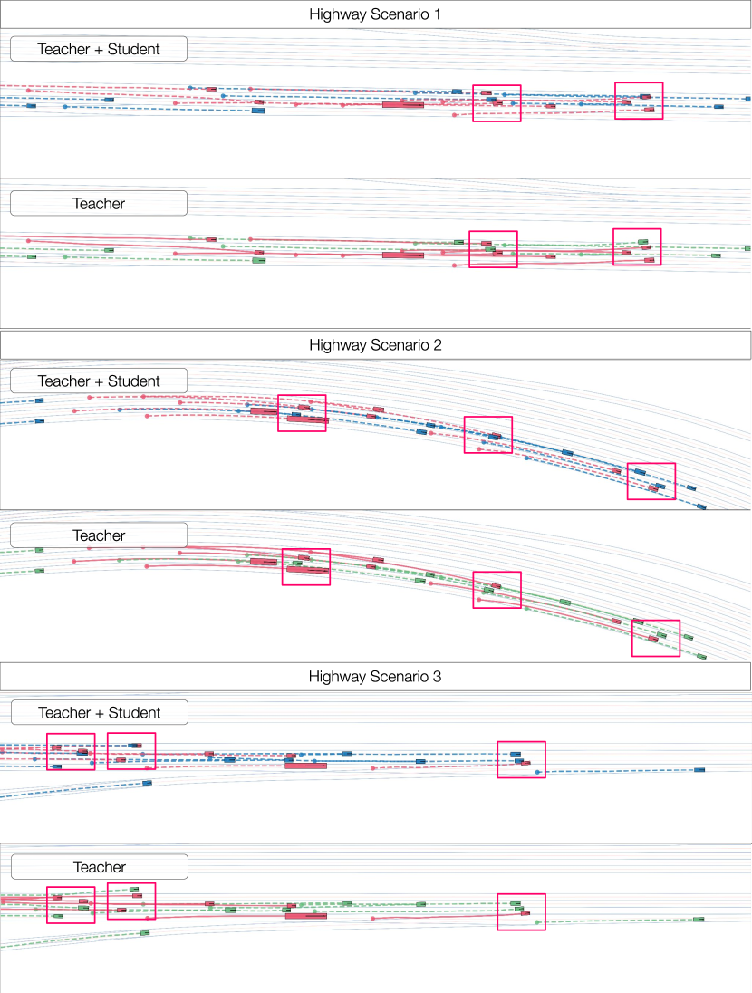
Figure 6: Qualitative Examples of scenarios discovered through our asymmetric self-play approach on Highway.

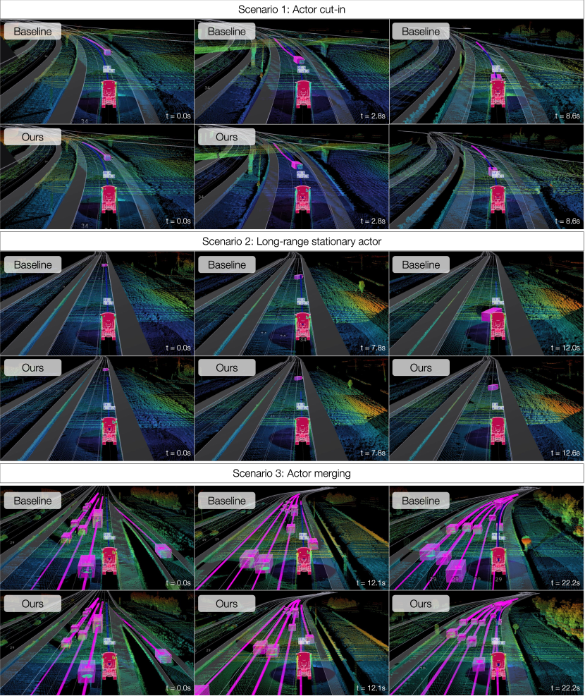
Figure 7: Qualitative Comparison for learned autonomy models. Top: Actor cut-in scenario for the Safety set. The baseline model trained only on real data does not react in time to the cut-in, resulting in a rear end collision. Our approach has had more exposure to these type of scenarios due to training with the teacher and has learned to react in time. Middle: Stationary actor scenario from the Safety set. The baseline model trained only on real data begins to slow down but is ultimately too late, resulting in an unavoidable collision. Our approach has learned that in order to avoid collision, it must react immediately, and comes to a stop in time. Bottom: A merge scenario from the Highway set. Both approaches are collision free, but we see our approach is more courteous, and slows down more for the merging actor.

References

- [1] Abeysirigoonawardena, Y., Shkurti, F., Dudek, G.: Generating adversarial driving scenarios in high-fidelity simulators. In: 2019 International Conference on Robotics and Automation (ICRA). pp. 8271–8277. IEEE (2019)
- [2] Agro, B., Sykora, Q., Casas, S., Urtasun, R.: Implicit occupancy flow fields for perception and prediction in self-driving. In: CVPR (2023)
- [3] Bakhtin, A., Wu, D.J., Lerer, A., Gray, J., Jacob, A.P., Farina, G., Miller, A.H., Brown, N.: Mastering the game of no-press diplomacy via human-regularized reinforcement learning and planning. In: ICLR (2023)
- [4] Bansal, M., Krizhevsky, A., Ogale, A.: Chauffeurnet: Learning to drive by imitating the best and synthesizing the worst. arXiv preprint arXiv:1812.03079 (2018)
- [5] Bergamini, L., Ye, Y., Scheel, O., Chen, L., Hu, C., Del Pero, L., Osiński, B., Grimmett, H., Ondruska, P.: Simnet: Learning reactive self-driving simulations from real-world observations. In: 2021 IEEE International Conference on Robotics and Automation (ICRA). pp. 5119–5125. IEEE (2021)
- [6] Berner, C., Brockman, G., Chan, B., Cheung, V., Debiak, P., Dennison, C., Farhi, D., Fischer, Q., Hashme, S., Hesse, C., Józefowicz, R., Gray, S., Olsson, C., Pachocki, J., Petrov, M., de Oliveira Pinto, H.P., Raiman, J., Salimans, T., Schlatter, J., Schneider, J., Sidor, S., Sutskever, I., Tang, J., Wolski, F., Zhang, S.: Dota 2 with large scale deep reinforcement learning. CoRR (2019)
- [7] Bernhard, J., Esterle, K., Hart, P., Kessler, T.: Bark: Open behavior benchmarking in multi-agent environments. In: 2020 IEEE/RSJ International Conference on Intelligent Robots and Systems (IROS). pp. 6201–6208. IEEE (2020)
- [8] Bhattacharyya, R.P., Phillips, D.J., Wulfe, B., Morton, J., Kuefler, A., Kochenderfer, M.J.: Multi-agent imitation learning for driving simulation. In: 2018 IEEE/RSJ International Conference on Intelligent Robots and Systems (IROS). pp. 1534–1539. IEEE (2018)
- [9] Biswas, S., Casas, S., Sykora, Q., Agro, B., Sadat, A., Urtasun, R.: Quad: Query-based interpretable neural motion planning for autonomous driving. In: ICRA (2024)
- [10] Bojarski, M., Del Testa, D., Dworakowski, D., Firner, B., Flepp, B., Goyal, P., Jackel, L.D., Monfort, M., Muller, U., Zhang, J., et al.: End to end learning for self-driving cars. arXiv preprint arXiv:1604.07316 (2016)
- [11] Bronstein, E., Srinivasan, S., Paul, S., Sinha, A., O’Kelly, M., Nikdel, P., Whiteson, S.: Embedding synthetic off-policy experience for autonomous driving via zero-shot curricula. arXiv preprint arXiv:2212.01375 (2022)
- [12] Cao, Y., Ivanovic, B., Xiao, C., Pavone, M.: Reinforcement learning with human feedback for realistic traffic simulation. arXiv preprint arXiv:2309.00709 (2023)
- [13] Cao, Y., Xu, D., Weng, X., Mao, Z., Anandkumar, A., Xiao, C., Pavone, M.: Robust trajectory prediction against adversarial attacks. In: Conference on Robot Learning. pp. 128–137. PMLR (2023)
- [14] Casas, S., Agro, B., Mao, J., Gilles, T., Cui, A., Li, T., Urtasun, R.: Detra: A unified model for object detection and trajectory forecasting. arXiv preprint (2024)
- [15] Casas, S., Sadat, A., Urtasun, R.: MP3: A unified model to map, perceive, predict and plan. In: CVPR (2021)
- [16] Chang, W.J., Pittaluga, F., Tomizuka, M., Zhan, W., Chandraker, M.: Controllable safety-critical closed-loop traffic simulation via guided diffusion. arXiv preprint arXiv:2401.00391 (2023)
- [17] Chen, B., Chen, X., Wu, Q., Li, L.: Adversarial evaluation of autonomous vehicles in lane-change scenarios. IEEE transactions on intelligent transportation systems 23(8), 10333–10342 (2021)
- [18] Codevilla, F., Müller, M., López, A., Koltun, V., Dosovitskiy, A.: End-to-end driving via conditional imitation learning. In: 2018 IEEE international conference on robotics and automation (ICRA). pp. 4693–4700. IEEE (2018)
- [19] Corso, A., Du, P., Driggs-Campbell, K., Kochenderfer, M.J.: Adaptive stress testing with reward augmentation for autonomous vehicle validatio. In: 2019 IEEE Intelligent Transportation Systems Conference (ITSC). pp. 163–168. IEEE (2019)
- [20] Cui, A., Casas, S., Wong, K., Suo, S., Urtasun, R.: Gorela: Go relative for viewpoint-invariant motion forecasting. arXiv preprint arXiv:2211.02545 (2022)
- [21] Ding, W., Cao, Y., Zhao, D., Xiao, C., Pavone, M.: Realgen: Retrieval augmented generation for controllable traffic scenarios. arXiv preprint arXiv:2312.13303 (2023)
- [22] Ding, W., Chen, B., Xu, M., Zhao, D.: Learning to collide: An adaptive safety-critical scenarios generating method. In: 2020 IEEE/RSJ International Conference on Intelligent Robots and Systems (IROS). pp. 2243–2250. IEEE (2020)
- [23] Ettinger, S., Cheng, S., Caine, B., Liu, C., Zhao, H., Pradhan, S., Chai, Y., Sapp, B., Qi, C.R., Zhou, Y., Yang, Z., Chouard, A., Sun, P., Ngiam, J., Vasudevan, V., McCauley, A., Shlens, J., Anguelov, D.: Large scale interactive motion forecasting for autonomous driving : The waymo open motion dataset. In: ICCV (2021)
- [24] Fremont, D.J., Kim, E., Dreossi, T., Ghosh, S., Yue, X., Sangiovanni-Vincentelli, A.L., Seshia, S.A.: Scenic: a language for scenario specification and data generation. Mach. Learn. (2023)
- [25] Gao, Y., Chen, J., Chen, X., Wang, C., Hu, J., Deng, F., Lam, T.L.: Asymmetric self-play-enabled intelligent heterogeneous multirobot catching system using deep multiagent reinforcement learning. IEEE Transactions on Robotics 39(4), 2603–2622 (2023)
- [26] Ghodsi, Z., Hari, S.K.S., Frosio, I., Tsai, T., Troccoli, A., Keckler, S.W., Garg, S., Anandkumar, A.: Generating and characterizing scenarios for safety testing of autonomous vehicles. In: 2021 IEEE Intelligent Vehicles Symposium (IV). pp. 157–164. IEEE (2021)
- [27] Gulino, C., Fu, J., Luo, W., Tucker, G., Bronstein, E., Lu, Y., Harb, J., Pan, X., Wang, Y., Chen, X., Co-Reyes, J.D., Agarwal, R., Roelofs, R., Lu, Y., Montali, N., Mougin, P., Yang, Z., White, B., Faust, A., McAllister, R., Anguelov, D., Sapp, B.: Waymax: An accelerated, data-driven simulator for large-scale autonomous driving research. In: NeurIPS (2023)
- [28] Hanselmann, N., Renz, K., Chitta, K., Bhattacharyya, A., Geiger, A.: King: Generating safety-critical driving scenarios for robust imitation via kinematics gradients. In: European Conference on Computer Vision. pp. 335–352. Springer (2022)
- [29] Harmel, M., Paras, A., Pasternak, A., Linscott, G.: Scaling is all you need: Training strong policies for autonomous driving with jax-accelerated reinforcement learning. arXiv preprint arXiv:2312.15122 (2023)
- [30] He, K., Zhang, X., Ren, S., Sun, J.: Deep residual learning for image recognition. In: Proceedings of the IEEE conference on computer vision and pattern recognition. pp. 770–778 (2016)
- [31] Henaff, M., Canziani, A., LeCun, Y.: Model-predictive policy learning with uncertainty regularization for driving in dense traffic. arXiv preprint arXiv:1901.02705 (2019)
- [32] Hoermann, S., Bach, M., Dietmayer, K.: Dynamic occupancy grid prediction for urban autonomous driving: A deep learning approach with fully automatic labeling. In: 2018 IEEE International Conference on Robotics and Automation (ICRA). pp. 2056–2063. IEEE (2018)
- [33] Igl, M., Kim, D., Kuefler, A., Mougin, P., Shah, P., Shiarlis, K., Anguelov, D., Palatucci, M., White, B., Whiteson, S.: Symphony: Learning realistic and diverse agents for autonomous driving simulation (2022). https://doi.org/10.48550/ARXIV.2205.03195
- [34] Kendall, A., Hawke, J., Janz, D., Mazur, P., Reda, D., Allen, J., Lam, V., Bewley, A., Shah, A.: Learning to drive in a day. CoRR (2018)
- [35] Klischat, M., Althoff, M.: Generating critical test scenarios for automated vehicles with evolutionary algorithms. In: 2019 IEEE Intelligent Vehicles Symposium (IV). pp. 2352–2358. IEEE (2019)
- [36] Koren, M., Alsaif, S., Lee, R., Kochenderfer, M.J.: Adaptive stress testing for autonomous vehicles. In: 2018 IEEE Intelligent Vehicles Symposium (IV). pp. 1–7. IEEE (2018)
- [37] LaValle, S.M.: Planning algorithms. Cambridge university press (2006)
- [38] Li, Q., Peng, Z., Feng, L., Zhang, Q., Xue, Z., Zhou, B.: Metadrive: Composing diverse driving scenarios for generalizable reinforcement learning. IEEE transactions on pattern analysis and machine intelligence 45(3), 3461–3475 (2022)
- [39] Liang, M., Yang, B., Hu, R., Chen, Y., Liao, R., Feng, S., Urtasun, R.: Learning lane graph representations for motion forecasting. In: Vedaldi, A., Bischof, H., Brox, T., Frahm, J. (eds.) Computer Vision - ECCV 2020 - 16th European Conference, Glasgow, UK, August 23-28, 2020, Proceedings, Part II. Lecture Notes in Computer Science, vol. 12347, pp. 541–556. Springer (2020). https://doi.org/10.1007/978-3-030-58536-5_32
- [40] Liang, M., Yang, B., Zeng, W., Chen, Y., Hu, R., Casas, S., Urtasun, R.: Pnpnet: End-to-end perception and prediction with tracking in the loop. In: Proceedings of the IEEE/CVF Conference on Computer Vision and Pattern Recognition. pp. 11553–11562 (2020)
- [41] Lioutas, V., Scibior, A., Wood, F.: Titrated: Learned human driving behavior without infractions via amortized inference. Transactions on Machine Learning Research (2022)
- [42] Loshchilov, I., Hutter, F.: Decoupled weight decay regularization. arXiv preprint arXiv:1711.05101 (2017)
- [43] Lu, Y., Fu, J., Tucker, G., Pan, X., Bronstein, E., Roelofs, B., Sapp, B., White, B., Faust, A., Whiteson, S., et al.: Imitation is not enough: Robustifying imitation with reinforcement learning for challenging driving scenarios. arXiv preprint arXiv:2212.11419 (2022)
- [44] Luo, W., Yang, B., Urtasun, R.: Fast and furious: Real time end-to-end 3d detection, tracking and motion forecasting with a single convolutional net. In: Proceedings of the IEEE conference on Computer Vision and Pattern Recognition. pp. 3569–3577 (2018)
- [45] Mahjourian, R., Kim, J., Chai, Y., Tan, M., Sapp, B., Anguelov, D.: Occupancy flow fields for motion forecasting in autonomous driving. IEEE Robotics and Automation Letters 7(2), 5639–5646 (2022)
- [46] Manivasagam, S., Wang, S., Wong, K., Zeng, W., Sazanovich, M., Tan, S., Yang, B., Ma, W.C., Urtasun, R.: Lidarsim: Realistic lidar simulation by leveraging the real world. In: Proceedings of the IEEE/CVF Conference on Computer Vision and Pattern Recognition. pp. 11167–11176 (2020)
- [47] Menzel, T., Bagschik, G., Maurer, M.: Scenarios for development, test and validation of automated vehicles. In: 2018 IEEE Intelligent Vehicles Symposium (IV). pp. 1821–1827. IEEE (2018)
- [48] Montali, N., Lambert, J., Mougin, P., Kuefler, A., Rhinehart, N., Li, M., Gulino, C., Emrich, T., Yang, Z., Whiteson, S., et al.: The waymo open sim agents challenge. Advances in Neural Information Processing Systems 36 (2024)
- [49] Ngiam, J., Caine, B., Vasudevan, V., Zhang, Z., Chiang, H.T.L., Ling, J., Roelofs, R., Bewley, A., Liu, C., Venugopal, A., et al.: Scene transformer: A unified architecture for predicting multiple agent trajectories. arXiv preprint arXiv:2106.08417 (2021)
- [50] Norden, J., O’Kelly, M., Sinha, A.: Efficient black-box assessment of autonomous vehicle safety. arXiv preprint arXiv:1912.03618 (2019)
- [51] O’Kelly, M., Sinha, A., Namkoong, H., Tedrake, R., Duchi, J.C.: Scalable end-to-end autonomous vehicle testing via rare-event simulation. Advances in neural information processing systems 31 (2018)
- [52] OpenAI, O., Plappert, M., Sampedro, R., Xu, T., Akkaya, I., Kosaraju, V., Welinder, P., D’Sa, R., Petron, A., Pinto, H.P.d.O., et al.: Asymmetric self-play for automatic goal discovery in robotic manipulation. arXiv preprint arXiv:2101.04882 (2021)
- [53] Peng, Z., Li, Q., Hui, K.M., Liu, C., Zhou, B.: Learning to simulate self-driven particles system with coordinated policy optimization. Advances in Neural Information Processing Systems 34, 10784–10797 (2021)
- [54] Philion, J., Peng, X.B., Fidler, S.: Trajeglish: Learning the language of driving scenarios. arXiv preprint arXiv:2312.04535 (2023)
- [55] Pomerleau, D.A.: Alvinn: An autonomous land vehicle in a neural network. Advances in neural information processing systems 1 (1988)
- [56] Qi, C.R., Su, H., Mo, K., Guibas, L.J.: Pointnet: Deep learning on point sets for 3d classification and segmentation. In: Proceedings of the IEEE conference on computer vision and pattern recognition. pp. 652–660 (2017)
- [57] Rempe, D., Philion, J., Guibas, L.J., Fidler, S., Litany, O.: Generating useful accident-prone driving scenarios via a learned traffic prior. In: Proceedings of the IEEE/CVF Conference on Computer Vision and Pattern Recognition. pp. 17305–17315 (2022)
- [58] Ross, S., Gordon, G., Bagnell, D.: A reduction of imitation learning and structured prediction to no-regret online learning. In: Proceedings of the fourteenth international conference on artificial intelligence and statistics. pp. 627–635. JMLR Workshop and Conference Proceedings (2011)
- [59] Sadat, A., Ren, M., Pokrovsky, A., Lin, Y.C., Yumer, E., Urtasun, R.: Jointly learnable behavior and trajectory planning for self-driving vehicles. In: 2019 IEEE/RSJ International Conference on Intelligent Robots and Systems (IROS). pp. 3949–3956. IEEE (2019)
- [60] Sadat, A., Segal, S., Casas, S., Tu, J., Yang, B., Urtasun, R., Yumer, E.: Diverse complexity measures for dataset curation in self-driving. In: IROS (2021)
- [61] Ścibior, A., Lioutas, V., Reda, D., Bateni, P., Wood, F.: Imagining the road ahead: Multi-agent trajectory prediction via differentiable simulation. In: 2021 IEEE International Intelligent Transportation Systems Conference (ITSC). pp. 720–725. IEEE (2021)
- [62] Seff, A., Cera, B., Chen, D., Ng, M., Zhou, A., Nayakanti, N., Refaat, K.S., Al-Rfou, R., Sapp, B.: Motionlm: Multi-agent motion forecasting as language modeling. In: Proceedings of the IEEE/CVF International Conference on Computer Vision. pp. 8579–8590 (2023)
- [63] Silver, D., Schrittwieser, J., Simonyan, K., Antonoglou, I., Huang, A., Guez, A., Hubert, T., Baker, L., Lai, M., Bolton, A., et al.: Mastering the game of go without human knowledge. nature 550(7676), 354–359 (2017)
- [64] Sinha, A., O’Kelly, M., Tedrake, R., Duchi, J.C.: Neural bridge sampling for evaluating safety-critical autonomous systems. Advances in Neural Information Processing Systems 33, 6402–6416 (2020)
- [65] Sukhbaatar, S., Denton, E., Szlam, A., Fergus, R.: Learning goal embeddings via self-play for hierarchical reinforcement learning. arXiv preprint arXiv:1811.09083 (2018)
- [66] Sukhbaatar, S., Lin, Z., Kostrikov, I., Synnaeve, G., Szlam, A., Fergus, R.: Intrinsic motivation and automatic curricula via asymmetric self-play. arXiv preprint arXiv:1703.05407 (2017)
- [67] Sun, Q., Huang, X., Williams, B.C., Zhao, H.: Intersim: Interactive traffic simulation via explicit relation modeling. In: 2022 IEEE/RSJ International Conference on Intelligent Robots and Systems (IROS). pp. 11416–11423. IEEE (2022)
- [68] Suo, S., Regalado, S., Casas, S., Urtasun, R.: Trafficsim: Learning to simulate realistic multi-agent behaviors. In: Proceedings of the IEEE/CVF Conference on Computer Vision and Pattern Recognition (CVPR). pp. 10400–10409 (June 2021)
- [69] Suo, S., Wong, K., Xu, J., Tu, J., Cui, A., Casas, S., Urtasun, R.: Mixsim: A hierarchical framework for mixed reality traffic simulation. In: Proceedings of the IEEE/CVF Conference on Computer Vision and Pattern Recognition (CVPR). pp. 9622–9631 (June 2023)
- [70] Tang, Y.: Towards learning multi-agent negotiations via self-play. In: ICCV (2019)
- [71] Treiber, M., Hennecke, A., Helbing, D.: Congested traffic states in empirical observations and microscopic simulations. Physical Review E 62(2), 1805–1824 (aug 2000). https://doi.org/10.1103/physreve.62.1805
- [72] e. V., A.: Asam openscenario v2.0.0 (2024)
- [73] Vaswani, A., Shazeer, N., Parmar, N., Uszkoreit, J., Jones, L., Gomez, A.N., Kaiser, L., Polosukhin, I.: Attention is all you need (2017)
- [74] Vemprala, S., Kapoor, A.: Adversarial attacks on optimization based planners. In: 2021 IEEE International Conference on Robotics and Automation (ICRA). pp. 9943–9949. IEEE (2021)
- [75] Vinitsky, E., Lichtlé, N., Yang, X., Amos, B., Foerster, J.: Nocturne: a scalable driving benchmark for bringing multi-agent learning one step closer to the real world. arXiv preprint arXiv:2206.09889 (2022)
- [76] Vinyals, O., Babuschkin, I., Czarnecki, W.M., Mathieu, M., Dudzik, A., Chung, J., Choi, D.H., Powell, R., Ewalds, T., Georgiev, P., et al.: Grandmaster level in starcraft ii using multi-agent reinforcement learning. Nature 575(7782), 350–354 (2019)
- [77] Wachi, A.: Failure-scenario maker for rule-based agent using multi-agent adversarial reinforcement learning and its application to autonomous driving. arXiv preprint arXiv:1903.10654 (2019)
- [78] Wang, J., Pun, A., Tu, J., Manivasagam, S., Sadat, A., Casas, S., Ren, M., Urtasun, R.: Advsim: Generating safety-critical scenarios for self-driving vehicles. In: Proceedings of the IEEE/CVF Conference on Computer Vision and Pattern Recognition. pp. 9909–9918 (2021)
- [79] Weber, H., Bock, J., Klimke, J., Roesener, C., Hiller, J., Krajewski, R., Zlocki, A., Eckstein, L.: A framework for definition of logical scenarios for safety assurance of automated driving. Traffic injury prevention 20(sup1), S65–S70 (2019)
- [80] Werling, M., Ziegler, J., Kammel, S., Thrun, S.: Optimal trajectory generation for dynamic street scenarios in a frenet frame. In: 2010 IEEE international conference on robotics and automation. pp. 987–993. IEEE (2010)
- [81] Wilson, B., Qi, W., Agarwal, T., Lambert, J., Singh, J., Khandelwal, S., Pan, B., Kumar, R., Hartnett, A., Pontes, J.K., Ramanan, D., Carr, P., Hays, J.: Argoverse 2: Next generation datasets for self-driving perception and forecasting. In: NeurIPS Datasets and Benchmarks (2021)
- [82] Xu, D., Chen, Y., Ivanovic, B., Pavone, M.: Bits: Bi-level imitation for traffic simulation. In: 2023 IEEE International Conference on Robotics and Automation (ICRA). pp. 2929–2936. IEEE (2023)
- [83] Zeng, W., Luo, W., Suo, S., Sadat, A., Yang, B., Casas, S., Urtasun, R.: End-to-end interpretable neural motion planner. In: Proceedings of the IEEE/CVF Conference on Computer Vision and Pattern Recognition. pp. 8660–8669 (2019)
- [84] Zhang, C., Guo, R., Zeng, W., Xiong, Y., Dai, B., Hu, R., Ren, M., Urtasun, R.: Rethinking closed-loop training for autonomous driving. In: Computer Vision–ECCV 2022: 17th European Conference, Tel Aviv, Israel, October 23–27, 2022, Proceedings, Part XXXIX. pp. 264–282. Springer (2022)
- [85] Zhang, C., Tu, J., Zhang, L., Wong, K., Suo, S., Urtasun, R.: Learning realistic traffic agents in closed-loop. In: Conference on Robot Learning. pp. 800–821. PMLR (2023)
- [86] Zhang, Q., Hu, S., Sun, J., Chen, Q.A., Mao, Z.M.: On adversarial robustness of trajectory prediction for autonomous vehicles. In: Proceedings of the IEEE/CVF Conference on Computer Vision and Pattern Recognition. pp. 15159–15168 (2022)
- [87] Zhang, Z., Liniger, A., Dai, D., Yu, F., Van Gool, L.: Trafficbots: Towards world models for autonomous driving simulation and motion prediction. arXiv preprint arXiv:2303.04116 (2023)
- [88] Zhong, Z., Rempe, D., Chen, Y., Ivanovic, B., Cao, Y., Xu, D., Pavone, M., Ray, B.: Language-guided traffic simulation via scene-level diffusion. In: Conference on Robot Learning (2023)
- [89] Zhong, Z., Rempe, D., Xu, D., Chen, Y., Veer, S., Che, T., Ray, B., Pavone, M.: Guided conditional diffusion for controllable traffic simulation. In: 2023 IEEE International Conference on Robotics and Automation (ICRA). pp. 3560–3566. IEEE (2023)
- [90] Zhou, M., Luo, J., Villella, J., Yang, Y., Rusu, D., Miao, J., Zhang, W., Alban, M., Fadakar, I., Chen, Z., et al.: Smarts: An open-source scalable multi-agent rl training school for autonomous driving. In: Conference on Robot Learning. pp. 264–285. PMLR (2021)
- [91] Zhou, Y., Tuzel, O.: Voxelnet: End-to-end learning for point cloud based 3d object detection. In: Proceedings of the IEEE conference on computer vision and pattern recognition. pp. 4490–4499 (2018)
- [92] Zhou, Z., Ye, L., Wang, J., Wu, K., Lu, K.: Hivt: Hierarchical vector transformer for multi-agent motion prediction. In: Proceedings of the IEEE/CVF Conference on Computer Vision and Pattern Recognition (CVPR) (2022)