3D Modeling of Moist Convective Inhibition in Hydrogen-Dominated Atmospheres

Abstract

Many planets have hydrogen-dominated atmospheres, including sub-Neptune exoplanets, recently formed planets with primordial atmospheres, and the Solar System’s giant planets. Atmospheric convection behaves differently in hydrogen-rich atmospheres compared to higher mean molecular weight atmospheres due to compositional gradients of tracers. Previous 1D studies suggested that compositional gradients of condensing tracers in H₂-rich atmospheres can entirely shut-off convection when the tracer abundance exceeds a critical threshold, leading to the formation of radiative layers where the temperature decreases faster with height than in convective profiles. We use 3D convection-resolving simulations to determine if convection is inhibited in H₂-rich atmospheres when the tracer mixing ratio exceeds the critical threshold. Three simulation sets are performed with a water vapor tracer in H₂-rich atmospheres. First, we perform simulations initialized on saturated isothermal states and find that compositional gradients can destabilize isothermal states, leading to rapid convective mixing. Next, simulations initialized on adiabatic profiles show distinct, stable inhibition layers forming when the H₂O tracer exceeds the critical threshold defined by previous studies. Within the inhibition layers, a small amount of energy is transported through condensation and re-evaporation, contrary to previous findings. The thermal profile slowly relaxes to a steep radiative state, but radiative relaxation timescales are long. Lastly, we show that superadiabatic temperature profiles can remain stable when the tracer abundance is greater than the critical amount. Our results suggest stable layers driven by condensation-induced convective inhibition form in H₂-rich atmospheres, including those of sub-Neptune exoplanets.

1 Introduction

Sub-Neptune exoplanets, planets with radii between $\sim$ 1.5 - 4 Earth radii, are one of the most commonly detected types of exoplanets. However, the nature and interior structure of these exoplanets is still unknown. A commonly accepted model for sub-Neptune structure is a hydrogen-helium-dominated atmosphere over a rocky or icy core (Van Eylen et al., 2018). However, other possible structure have been proposed and include; “water worlds” (Luque & Pallé, 2022) which have high volatile fraction envelops, hot supercritical atmospheres containing a mixture of H₂ and H₂O (Pierrehumbert, 2023; Benneke et al., 2024), and “Hycean Worlds” (Madhusudhan et al., 2021) which are planets with shallow hydrogen-helium-dominated atmospheres overlaying a water rich interior and large oceans. Hydrogen-dominated atmospheres are also relevant for planets that have recently formed and still retain a transient hydrogen envelope (Young et al., 2023), and the solar system giant planets. In this work, we explore the atmospheric state of H₂-rich atmospheres to inform our understanding of sub-Neptunes and other planets with H₂-rich atmospheres

In $\rm H_{2}$-dominated atmospheres, vertical mixing due to convection behaves differently compared to higher mean molecular weight atmospheres, like that of Earth. Atmospheric convection plays a fundamental role in cloud processes, determining the vertical temperature structure, and transporting energy and atmospheric tracers (i.e. chemical constituents, hereafter called “tracers”) vertically within the atmosphere. The condensation of atmospheric tracers during convection, known as moist convection, plays a significant role in the formation of precipitation and cloud processes. Conversely, dry convection refers to convective mixing where atmospheric tracers are sub-saturated or do not undergo phase changes within the temperature-pressure range of the atmosphere. Convection arises due to gravity acting upon vertical variations of density within the atmosphere. Density variations are due to either temperature (thermal convection) or compositional (compositional convection) variations. Convection can arise in the atmosphere due to radiation heating the surface or cooling aloft, but could also arise from variations of compositional gradients of tracers due to condensation or chemical reactions (see Yang et al., 2019; Yang & Seidel, 2020; Guillot, 1995; Li & Ingersoll, 2015; Leconte et al., 2017; Daley-Yates et al., 2021; Habib & Pierrehumbert, 2024).

Atmospheric tracers have a higher mean molecular weight than the background atmosphere in H₂-dominated atmospheres. Therefore, a parcel of pure H₂ air will be less dense and lighter than a parcel containing a mixture of H₂ with any atmospheric tracer at the same temperature and pressure. Tracers in H₂-dominated atmospheres can strongly stabilize and potentially inhibit convection (Guillot, 1995; Leconte et al., 2017; Friedson & Gonzales, 2017). Habib & Pierrehumbert (2024) demonstrated through 3D convection-resolving simulations that compositional gradients of non-condensing tracers significantly stabilize and affect stable atmospheric states in H₂-dominated atmospheres.

Condensing compositional convection in H₂-dominated atmospheres has primarily been explored using 1D analytical models for applications to the Solar System giant planets (Guillot, 1995; Li & Ingersoll, 2015; Leconte et al., 2017; Friedson & Gonzales, 2017). Guillot (1995) found that convection is completely suppressed when the abundance of an atmospheric tracer exceeds a critical threshold in saturated, H₂-dominated atmospheres. Leconte et al. (2017) extended this theory and hypothesized that condensation-driven convective inhibition results in atmospheric stability against all vertical mixing, including double diffusive convection, and suggested radiation is the sole mechanism to transport heat though the atmosphere. Furthermore, Leconte et al. (2017) argued that in regions where the abundance of a saturated tracer exceeds the critical threshold defined by Guillot (1995), a radiative layer develops with a superadiabatic temperature profile where temperature decreases with height more rapidly than in a convective layer. Radiative layers imply that the deep internal temperature of H₂-dominated atmospheres is much hotter than it would be under a purely convective atmospheric profile, assuming the temperature at the top of the atmosphere is the same. In their analytical model, Leconte et al. (2017) suggest the structure of H₂-rich atmospheres consists of a deep dry convective region, overlaid by a radiative superadiabatic region, and topped by a condensing, moist convective region.

Several recent papers have applied the hypothesis that superadiabatic layers form due to compositional convective inhibition in H2-rich atmospheres, focusing on Hycean worlds and magma ocean planets. Innes et al. (2023) used a 1D radiative-convective model, where the temperature profile was set to be superadiabatic when the saturated water vapor tracer mixing ratio exceeded a critical threshold, to predict whether a water ocean could exist under an H${}_{2}-$rich atmosphere. Their model suggests that current sub-Neptune targets are unlikely to host surface water oceans because superadiabatic layers cause deep internal atmospheric temperatures to be too high to sustain liquid water. Additionally, Misener & Schlichting (2022) and Markham et al. (2022) explored compositional convective inhibition due to silicate vapor in magma ocean planets with H${}_{2}-$-atmospheres. Misener & Schlichting (2022) found that radiative layers decrease the overall radius of sub-Neptune planets compared to planets assumed to be fully convective. Markham et al. (2022) studied core-envelope interactions in magma ocean planets and suggested that the core is much hotter due to compositional convective inhibition from silicate vapors, leading to a supercritical core and inefficient cooling of these planets.

In this work, we aim to test the hypothesis proposed by Leconte et al. (2017). 1D radiative-convective models allow for fast exploration of planetary structure. However, 1D models are limited and often do not account for the effects of sub-saturation of the tracer, re-evaporation of condensates, or turbulent mixing. We aim to explore the robustness of superadiabatic layers while accounting for the processes that are neglected in 1D atmospheric models. Using 3D convection-permitting simulations, we explore the atmospheric temperature and compositional structure in H₂-dominated atmospheres when the tracer abundance exceeds a critical threshold. 3D convection permitting simulations also allow us to determine the convectively stable states that emerge from the initial conditions. Our objectives are to answer the following questions:

• Is convection suppressed when the tracer abundance surpasses the critical threshold defined by Guillot (1995)?

• If convectively stable regions form, is the temperature profile in these regions superadiabatic? Do 3D convection-permitting simulations support the atmospheric structure proposed by Leconte et al. (2017)?

• How does condensation influence the atmospheric heat and moisture transport if convection is inhibited?

We perform 3D simulations using Cloud Model 1 v20.3 (CM1 Bryan, 2009) to study a saturated water vapor tracer in an $\rm H_{2}$-dominated atmosphere, allowing for tracer condensation and incorporating radiation effects through a gray gas radiation scheme. We perform a set of simulations initialized in three distinct conditions: saturated isothermal atmosphere, an initially adiabatic setup, and a saturated superadiabatic profile. Overall, our simulation results show distinct convectively stable regions do form where the atmosphere is saturated and the tracer abundance is greater than the critical threshold.

Recently, Leconte et al. (2024) utilized 3D convection-permitting simulations to explore the formation of convectively stable regions when vapor abundance exceeds a critical threshold. Their findings confirm that convectively stable regions form, and their model replicates the atmospheric structure proposed by Leconte et al. (2017), where a moist convective layer overlies a radiative superadiabatic region, which in turn caps a dry convection layer. Moreover, Leconte et al. (2024) find that the tracer is still transported upwards through the convectively stable region through turbulent mixing. Our study uses a different convection-resolving model compared to Leconte et al. (2024), with distinct formulations of the equation of state and conservation of energy in the two numerical models. Additionally, we use a slightly different model setup compared to Leconte et al. (2024) who specifically modeled the sub-Neptune K2-18b. In contrast, our study is more generalized and explores different initializations. We compare our simulation results with those presented by Leconte et al. (2024) in Section 4.

Understanding the atmospheric state of planets with $\rm H_{2}$-dominated atmospheres improves our ability to represent convection in global general circulation models and to better interpret observations of these worlds. While the simulations presented in this work focus on H₂O tracer in $\rm H_{2}$-dominated atmospheres, convective inhibition due to condensing compositional convection is relevant for any planetary atmosphere with a condensable tracer that has a higher mean molecular weight than the background atmosphere. Examples where condensation-driven convective inhibition is important include water and ammonia in sub-Neptune exoplanets, silicates in magma ocean planets (e.g. Misener & Schlichting, 2022; Markham et al., 2022), methane and water vapor in Uranus and Neptune’s atmosphere (Irwin et al., 2022), and water vapor in Saturn’s atmosphere (Li & Ingersoll, 2015).

In section 2 we review the condensing compositional convection stability criterion. In section 3 we describe our CM1 simulation setup, and present our simulation results and discussions in section 4.

2 A review of the convective stability criterion with compositional effects

We will consider mixtures of a non-condensing background gas, with corresponding quantities labeled with subscript $b$, with a second gas, the tracer, that can condense within the atmosphere denoted by subscript $v$ (for “vapor”). The effects of tracers on convection (also called virtual effects) are typically represented using virtual temperature,

$$T_{v}=T\left(\frac{1+q_{v}/\epsilon}{1+q_{v}}\right),$$ (1)

where $T$ is the atmospheric temperature (K), $q_{v}$ is the vapor mixing ratio of the atmospheric tracer (kg/kg), and $\epsilon=M_{v}/M_{b}$ is the ratio of the mean molecular weight of the tracer to the background atmosphere (Emanuel, 1994). Effectively, $T_{v}$ represents density in units of temperature and allows us to write the ideal gas law as $p=\rho R_{b}T_{v}$ where $p$ is the total atmospheric pressure, $R_{b}$ is the gas constant for the background atmosphere and $\rho$ is the total atmospheric density. The vapor mixing ratio quantifies how much atmospheric tracer is present relative to the background air and is defined as the ratio of the density of the tracer ($\rho_{v}$) relative to the background atmosphere density ($\rho_{b}$),

$$q_{v}=\rho_{v}/\rho_{b}.$$ (2)

If the atmospheric tracer has a lower mean molecular weight than the bulk atmosphere $\epsilon<1$, then $T_{v}>T$ and the atmospheric tracer can enhance buoyancy relative to a parcel of pure background atmosphere at the same temperature. Conversely, when $\epsilon>1$ and the atmospheric tracer is heavier than the background atmosphere and it can suppress convection from occurring. For instance, in a H₂-dominated atmospheres with a water vapor tracer $\epsilon=8.9$.

In the absence of condensation, stability against convection can be approximated by;

$$\frac{d\ln T_{v,\rm amb}}{d\ln p}\leq\beta_{\rm mix},$$ (3)

where $T_{v,\rm amb}$ is the virtual temperature profile of the ambient atmosphere, $p$ is the atmospheric pressure, and $\beta_{\rm mix}\equiv\frac{R}{C_{p}}$ where $R$ and $C_{p}$ are a representative gas constant and heat capacity for the mixture of tracer with the background atmosphere. Eqn. 3 is a form of the Ledoux criterion for local stability (Ledoux, 1947) and describes the stability against infinitesimal displacements of a parcel containing a mixture of the bulk atmosphere and a non-condensing tracer (Habib & Pierrehumbert, 2024).

When the atmospheric tracer can condense in the temperature-pressure range of the atmosphere, then a key difference to the non-condensing case, is that the vapor mixing ratio profile is constrained by the temperature through the saturation vapor pressure. Assuming that the density of condensates is much greater than the gas density, the Clausius-Clapeyron equation allows us to determine the saturation vapor pressure as,

$$\frac{d\ln e_{\rm sat}}{d\ln T}=\frac{L_{v}}{R_{v}T},$$ (4)

where $e_{\rm sat}$ is the saturation vapor pressure of the condensable tracer at a given temperature $T$, $L_{v}$ is the latent heat of vaporization, and $R_{v}$ is the gas constant of the condensable tracer. For a given temperature, we can determine the vapor mixing ratio at which the tracer is saturated,

$$q_{v,\rm sat}=\epsilon\left(\frac{e_{\rm sat}}{p-e_{\rm sat}}\right).$$ (5)

To determine if the tracer is saturated at a given $(p,T)$, we compare the partial pressure of the tracer to its saturation vapor pressure,

$$RH=\frac{p_{v}}{e_{\rm sat}}=\left(\frac{q_{v}}{\epsilon+q_{v}}\right)\left(\frac{p}{e_{\rm sat}}\right)$$ (6)

where $p_{v}$ is the partial pressure of the tracer at $(p,T)$ and $RH$ is the relative humidity.

Assuming the saturated air parcel is displaced approximately adiabatically without any mixing with its surroundings,

$$\frac{d\ln{T^{*}_{ad}}}{d\ln{P}}=\beta_{\rm mix}\left[\frac{1+q_{v,\rm sat}\left(\frac{L_{v}}{R_{b}T}\right)}{1+q_{v,\rm sat}\left(\frac{L_{v}}{C_{p,\rm mix}T}\right)\left(\frac{L}{R_{v}T}\right)\left(\frac{1+q_{v,\rm sat}/\epsilon}{1+q_{v,\rm sat}}\right)}\right].$$ (7)

Eqn. 7 is the moist pseudoadiabat and gives the temperature-pressure profile of a saturated air parcel as it is displaced (Emanuel, 1994). Similar to Guillot (1995); Leconte et al. (2017), we assume the volume of the condensed phase is negligible compared to the vapor phase of the atmospheric tracer, and all condensed phases are instantaneously removed. We do not consider the compositional gradient of condensed phases in determining atmospheric stability in this work.

To determine the stability of a saturated atmosphere to convection, considering compositional gradients, we need to examine how condensation affects the mean molecular weight gradient of both a displaced air parcel and the surrounding atmosphere. As a saturated air parcel is displaced, condensation leads to a change in the composition of the parcel. Moreover, the surrounding saturated atmosphere exhibits a compositional gradient because the vapor mixing ratio changes with altitude, following the saturation vapor pressure curve. The compositional gradient is given by,

$$\frac{d\ln{\mu}}{d\ln{p}}=q_{v,\rm sat}\left(\frac{1-1/\epsilon}{1+q_{v,\rm sat}}\right)\left[\left(\frac{L_{v}}{R_{v}T}\right)\left(\frac{d\ln{T}}{d\ln{p}}\right)-1\right],$$ (8)

where $\mu$ is the total mean molecular weight of the atmosphere (Guillot, 1995; Leconte et al., 2017).

Stability to convection can be determined by comparing the density, or virtual temperature, of a displaced saturated air parcel to that of the surrounding saturated atmosphere. To compare the virtual temperature directly, we would need to solve Eqn. 8 and Eqn. 7 and account for the change in the composition of the displaced air parcel due to condensation. Alternatively, we consider stability against infinitesimal displacements and compare the gradient of virtual temperature of a saturated parcel to that of the ambient saturated atmosphere where $\frac{d\ln{T_{v}}}{d\ln{p}}=\frac{d\ln{T}}{d\ln{p}}-\frac{d\ln{\mu}}{d\ln{p}}$. A saturated parcel is stable against infinitesimal displacements when,

$$\left(\frac{d\ln{T}}{d\ln{p}}-\frac{d\ln{\mu}}{d\ln{p}}\right)\Bigg{\rvert}_{\rm amb}-\left(\frac{d\ln{T}}{d\ln{p}}-\frac{d\ln{\mu}}{d\ln{p}}\right)\Bigg{\rvert}_{\rm parcel}\leq 0$$ (9)

where $\left(\frac{d\ln{T}}{d\ln{p}}\right)\big{\rvert}_{\rm parcel}$ = $\frac{d\ln{T^{*}_{\rm ad}}}{d\ln{p}}$ is the temperature gradient of the saturated parcel given by the moist adiabat, and $\left(\frac{d\ln{T}}{d\ln{p}}\right)\big{\rvert}_{\rm amb}$ is the temperature gradient of the background atmosphere. $\frac{d\ln{\mu}}{d\ln{p}}$ is given by Eqn. 8 and can be evaluated for the parcel and ambient atmosphere using $\frac{d\ln{T^{*}_{\rm ad}}}{d\ln{p}}$ and $\left(\frac{d\ln{T}}{d\ln{p}}\right)\big{\rvert}_{\rm amb}$ respectively.

Simplifying Eqn. 9 using Eqn. 8 yields,

$$\left(\nabla_{\rm amb}-\nabla^{*}_{\rm ad}\right)\left(1-\left(\frac{q_{v,\rm sat}}{1+q_{v,\rm sat}}\right)(1-1/\epsilon)\left(\frac{L_{v}}{R_{v}T}\right)\right)\leq 0,$$ (10)

where $\nabla=\frac{d\ln{T_{x}}}{d\ln{p}}$, “amb” represents the atmospheric temperature gradient and the “^∗ad” represents the temperature gradient defined by the moist adiabat. Eqn. 10 is the Guillot criterion for local stability against condensing compositional convection (Guillot, 1995).

When the atmospheric tracer is lighter than the background atmosphere so that $\epsilon~{}<~{}1$, the mean molecular weight term, $(1-1/\epsilon)$ will always be negative meaning that the compositional term in Eqn. 10 (second bracket) is always positive. Conversely, when $\epsilon~{}>~{}1$, a compositional gradient can stabilize an unstable atmospheric temperature. Consider $\nabla_{\rm amb}>\nabla^{*}_{\rm ad}$, in the absence of a compositional gradient the ambient temperature profile is unstable and convection will occur. However, when accounting for the compositional effects, the compositional gradient can stabilize an unstable atmosphere to infinitesimal displacements and inhibit convection when $q_{v,\rm sat}\geq q_{\rm crit}$ where

$$q_{\rm crit}=\frac{R_{v}T}{L_{v}(1-1/\epsilon)-R_{v}T}$$ (11)

(Guillot, 1995). Compositional gradients of condensable tracers in $\rm H_{2}$-dominated atmospheres can provide a strong stabilizing mean molecular weight gradient that can inhibit convection entirely when $q_{v}\geq q_{\rm crit}$.

In this work, we use 3D convection-permitting simulations to explore the atmospheric structure when accounting for compositional stabilization in $\rm H_{2}$-dominated atmospheres. Leconte et al. (2017) suggested that when convection is inhibited, a radiative superadiabatic layer would form between the upper and lower atmosphere which are convective. We use 3D simulations to determine if this result is realized and explore condensation as a mechanism to transport heat between stable atmospheric layers.

3 Compositional Convection Modeling with CM1

We use Cloud Model 1 (CM1 Bryan, 2009) to perform idealized simulations of condensing compositional convection. CM1 is a non-hydrostatic convection-resolving model that has been extensively used to study atmospheric flows. In this work, we utilize CM1 version 20.3 from Habib & Pierrehumbert (2024), which incorporates modifications to the original code that include setting the thermodynamic constants and planetary parameters using an input file, and revising the buoyancy equation to account for non-dilute concentrations of atmospheric tracers.

Table 1: Atmospheric constants used within the CM1 condensing compositional convection simulations

	$\rm C_{p}$	$\rm C_{v}$	R	$\rm\varepsilon=M_{v}/M_{b}$	$\kappa$
	J kg-1 K-1	J kg-1 K-1	J kg-1 K-1		$\rm m^{2}kg^{-1}$
Hydrogen (Background Atmosphere)	14304.0	10160.0	4144.0	8.94	$1.18\times 10^{-4}$
Water Vapor (Atmospheric tracer)	1870.0	1408.5	461.5	N/A	0.01

The thermodynamic constants used in this study are listed in Table 1. Gravity is set to 9.8 m/s² in all simulations. We run CM1 using the fully compressible equations in Large-Eddy Simulation (LES) mode. Sub-grid scale turbulent mixing is included using a turbulent kinetic energy closure (Deardorff, 1980) to parameterize mixing at unresolved scales similar to previous studies (Tan et al., 2021; Lefèvre et al., 2022; Habib & Pierrehumbert, 2024). We use a rigid bottom boundary condition, and horizontal periodic boundary conditions. Additionally, we apply a Rayleigh dampening layer in the top 10 km of the domain to damp out any upward propagating gravity waves. We use a timestep of 3 seconds, and perform the radiative calculation once per minute.

We use the TWOSTR (Kylling et al., 1995) numerical package to solve the gray gas radiative transfer equations. TWOSTR is a two stream plane-parallel radiative transfer model that uses a gray gas approximation. We assume a constant background opacity of $\kappa_{b}=1.18\times 10^{-4}\;\rm{m^{2}\;kg^{-1}}$ and a constant water vapor opacity of $\kappa_{v}=0.01\;\rm{m^{2}\;kg^{-1}}$ based on previous studies (Menou, 2011; Freedman et al., 2014; Innes et al., 2023). The total opacity $\kappa$ varies as a function of pressure $p$ and is determined by,

$$\kappa(p)=\frac{\kappa_{b}+\kappa_{v}*q_{v}(p)}{1+q_{v}},$$ (12)

where $q_{v}$ is the vapor mixing ratio of the atmospheric tracer, $\kappa_{b}$ and $\kappa_{v}$ are the opacity of the background air and atmospheric tracer, respectively. Additionally, we neglect shortwave heating of the upper atmosphere and the effects of scattering. We use a rigid lid bottom boundary condition with a fixed surface temperature. We run CM1 with no moisture, evaporative, surface fluxes. The turbulent heat and momentum exchange at the bottom boundary is calculated using the original CM1 formulation. In our modeling setup, the atmosphere is assumed to be transparent to shortwave radiation. The radiation setup differs from sub-Neptune exoplanets, where the atmosphere is largely heated by in-situ shortwave absorption. We opted for a simplified setup where convection can occur, allowing us to capture the effects of radiation on the temperature profile without the complexity and computational demand of a more realistic radiative transfer scheme. Our CM1 setup represents a sub-Neptune with a deep interior containing water vapor, but without a condensed ocean reservoir at the bottom.

We use the Rotunno & Emanuel (1987) condensation scheme to account for condensation of the water vapor tracer, rainout and evaporation. We only consider the vapor and liquid phase in this work. Within the Rotunno and Emanuel condensation scheme, the vapor mixing ratio is, $q_{v}=\frac{\rho_{v}}{\rho_{b}}$, and the liquid condensate is $q_{l}=\frac{\rho_{l}}{\rho_{b}}$, where $\rho_{l}$ is the density of liquid condensate, $\rho_{b}$ is the background atmosphere density, and $\rho_{v}$ is the density of the atmospheric tracer in vapor form. Further, in this scheme a distinction is made between cloud and rain water. Condensate with $q_{l}\leq 1g\;kg^{-1}$ is cloud condensate and has a terminal fall velocity of V = 0 $\rm m\;s^{-1}$, while condensates with $q_{l}>1g\;kg^{-1}$ is rain condensate and has a terminal fall velocity of V = 10 $\rm m\;s^{-1}$.

Condensation is modeled as a two-step process where first, precipitation occurs in situ and second, the condensate is removed by rainout if $V>0$. Condensation occurs at a given timestep when $q_{v}(p)>q_{v,\rm sat}(p)$ where $q_{v,\rm sat}(p)$ is the vapor mixing ratio if the air parcel at the given $(T,p)$ is fully saturated. In this scheme, condensation occurs to remove excess water vapor relative to saturation such that after condensation $q_{v}(p)~{}=~{}q_{v,\rm sat}(p)$. When condensation occurs, a small amount of liquid condensate forms, the vapor pressure of the tracer is adjusted to the saturation vapor pressure, and the latent heat release of condensation causes the local temperature to increase slightly. Condensates can evaporate in a grid cell if $q_{v}(p)<q_{v,\rm sat}(p)$ and $q_{l}>0$. Evaporation occurs until the condensate is depleted or $q_{v}(p)=q_{v,\rm sat}(p)$, depending on which occurs first. Rainout moves condensates to lower atmospheric layers, where they would evaporate if the layers are sub-saturated. When evaporation occurs, the temperature decreases slightly due to the latent heat required to evaporate the liquid, and the vapor pressure of the tracer is again adjusted accordingly. We do not model detailed cloud condensation growth or microphysics. Condensates are assumed to fall out instantaneously and re-evaporated in sub-saturated regions.

We perform three sets of condensing compositional convection simulations in this work. First, we model a saturated isothermal atmosphere. In the saturated isothermal simulations, we anticipate rapid convection to stabilize the system, but our goal is to determine whether the system can evolve to a final atmospheric state that is non-adiabatic. Without compositional effects, isothermal atmospheres are stable to convection. The destabilization of isothermal layers is an important novel feature, particularly since the lower portions of thick atmospheres in pure radiative equilibrium often exhibit isothermal radiative layers. Second, we perform condensing compositional convection simulations which are initialized on adiabatic profiles. Here, we explore if layer(s) of convective inhibition can form and how this impacts stable end-states of the temperature and compositional profile. In particular, we aim to determine if a stable superadiabatic layer can form and whether 3D simulations support the atmospheric structure suggested by Leconte et al. (2017). Lastly, we perform a simulation initialized on a saturated superadiabatic profile to determine if saturated superadiabatic states are stable over time when $q_{v,\rm sat}\geq q_{\rm crit}$. The CM1 setup for the isothermal, adiabatic, and superadiabatic simulations are described in the following sections respectively and summarized in Table 2.

Table 2: Initial atmospheric sounding parameters and domain size used for the CM1 condensing compositional convection simulations. Note, $L_{x}$ and $L_{z}$ are the horizontal domain width and vertical domain height respectively. The horizontal domain is a square such that $L_{x}$ = $L_{y}$, and the horizontal resolution is the same in the x and y direction.

	$\rm P_{s}$	$\rm T_{s}$	$\rm q_{v,s}$	$\rm q_{crit}$	$\rm L_{x}$	$\rm L_{z}$	nx	nz	Time
	[bar]	[K]	[kg/kg]	[kg/kg]	[km]	[km]			[days]
Initial Isothermal Simulations
No Radiation and $q_{v}\approx q_{\rm crit}$	1	273	0.055	0.057	1152	350	192	70	58
$q_{v}\approx q_{\rm crit}$	1	273	0.055	0.057	1152	350	192	70	58
$q_{v}>q_{\rm crit}$	1	300	0.321	0.062	1152	150	192	30	116
$q_{v}<q_{\rm crit}$	20	300	0.016	0.062	1152	525	192	105	116
Initial Adiabatic Simulations
Dry then Moist Adiabat	1	450	0.2	0.1	1200	500	192	250	1200
Moist Adiabat	1	300	0.2	0.1	1200	400	192	200	600
Initial Superadiabatic Simulations
Superadiabatic	1	315	0.8	0.1	384	200	192	200	600

3.1 Isothermal Condensing Compositional Convection Simulations

We performed a set of four isothermal simulations. All simulations were initialized with the assumption that the atmosphere is saturated throughout. Given that the initial temperature is constant across the domain, a saturated isothermal profile implies an increase in the vapor mixing ratio as pressure decreases. This effect is mathematically represented in Eqn. 5. Here, if $T$ is constant, then $e_{\rm sat}$ remains constant, and as pressure decreases, $q_{v,\rm sat}$ increases. However, increasing $q_{v,\rm sat}$ indefinitely will eventually cause CM1 to become numerically unstable. Therefore, we set an arbitrary cutoff for the top of the atmosphere in these simulations to be at the point where $q_{v,\rm sat}=1$, corresponding to 50% water by mass. This definition means that the simulation domain height depends on the isothermal temperature we set for the atmosphere.

For all of our saturated isothermal cases, the initial atmospheric state is unstable to non-condensing compositional convection by the Ledoux criterion. This is because $q_{v}(p)$ is increasing with height, the temperature is constant, and the tracer is denser than the background air, therefore a denser fluid is resting above a lighter fluid. Further, atmospheric stability against moist compositional convection can be determined by considering the Guillot criterion given by Eqn. 10. In the case of an isothermal atmosphere, $(\nabla_{\rm amb}-\nabla^{*}_{\rm ad})<0$. Therefore, the initial atmospheric state is locally stable against convection by the Guillot criterion when $q_{v}(p)\leq q_{\rm crit}$ and unstable when $q_{v}(p)>q_{\rm crit}$.

We perform three saturated isothermal test cases where we set the atmospheric temperature such that the surface saturated vapor mixing ratio, $q_{v,\rm sat}(p_{s})$, is approximately equal, greater than, and less than the surface critical vapor mixing ratio $q_{\rm crit}(T_{s})$ given by Eqn. 11. Specifically, we run simulations at

1. $T$ = 273 K, $p_{s}$ = 1 bar, and $q_{v,\rm sat}(p_{s})~{}\approx~{}q_{\rm crit}(T_{s})$.

2. $T$ = 300 K, $p_{s}$ = 1 bar, and $q_{v,\rm sat}(p_{s})~{}>~{}q_{\rm crit}(T_{s})$,

3. $T$ = 300 K, $p_{s}$ = 20 bar, and $q_{v,\rm sat}(p_{s})~{}<~{}q_{\rm crit}(T_{s})$,

We also run the 273 K test case without radiation as a control test case where the final state is solely representative of condensing compositional convection. For the case where $q_{v,\rm sat}(p_{s})<q_{\rm crit}(T_{s})$, the surface pressure was adjusted to maintain the atmospheric temperature in a regime where condensation occurs while ensuring that the initial condition $q_{v,\rm sat}(p_{s})<q_{\rm crit}(T_{s})$ was met.

In the $q_{v,\rm sat}(p_{s})>q_{\rm crit}$ simulation, the initial atmospheric state is unstable to both moist and dry compositional convection. Conversely, in the $q_{v,\rm sat}(p_{s})<q_{\rm crit}$ the initial atmospheric state is locally stable to condensing compositional convection in the region where $q_{v,\rm sat}(p_{s})<q_{\rm crit}$ and unstable to dry compositional convection by the Ledoux criterion. In the $q_{v,\rm sat}(p_{s})<q_{\rm crit}$ case we are testing if condensation can stabilize the atmospheric state. The initial conditions were chosen to highlight the compositional destabilization and the nature of evolution towards an end state. The domain size, resolution, and simulation time for the CM1 test cases are given in Table 2.

3.2 Adiabatic Condensing Compositional Convection Simulations

We performed two adiabatic condensing compositional convection simulations, which were initialized as follows: (1) with the entire atmosphere set to a moist adiabat defined by Eqn 7, and (2) with the lower atmosphere following a dry adiabat with a constant $q_{v}=0.2$ kg/kg until the point of saturation, after which the temperature profile transitions to a moist adiabat. When the temperature in the upper atmosphere reached 150 K, the temperature profile was set to be isothermal emulating a radiative stratosphere. The dry adiabat describes the temperature profile of an atmosphere that is well-mixed and the tracer is either sub-saturated or non-condensing in the temperature-pressure range of the atmosphere. The dry adiabat is defined as,

$$\frac{d\ln{T_{\rm ad}}}{d\ln{p}}=-\frac{R}{C_{p}},$$ (13)

where $R$ and $C_{p}$ are the gas constant and heat capacity for the well-mixed region. The CM1 test case initialized on a dry then moist adiabat is qualitatively a sub-Neptune model with a sub-saturated non-condensing convective deep atmosphere, which becomes saturated and condensing in the colder upper atmosphere. The moisture reservoir is the sub-saturated deep layer, rather than a liquid ocean. Both adiabatic simulations are initialized such that $q_{v,s}>q_{\rm crit}(T_{s})$.

With the adiabatic simulations, we are exploring whether superadiabatic layers can form and testing the hypothesis of Leconte et al. (2017). The goal of these simulations is to determine whether a superadiabatic temperature profile will form in between the dry and moist convection regions where convection should be inhibited according to the Guillot criterion. The domain size, resolution, and simulation duration for the CM1 test cases are summarized in Table 2.

3.3 Superadiabatic Condensing Compositional Convection Simulation

Lastly, we perform a single simulation that is initialized on a saturated superadiabatic temperature profile defined by,

$$T=T_{s}\left(\frac{1+e^{-z/H}}{2}\right)^{1/4},$$ (14)

where $T_{s}$ is the surface temperature set to 315 K, $z$ is the domain height, and $H$ is a reference vertical scale height that was set to 26 km. The temperature profile was set such that the initial state is superadiabatic, the temperature decreases faster with height compared to an adiabatic profile, in the lower atmosphere. The initial tracer mixing ratio was set such that the the atmosphere is fully saturated in the lower domain. In the upper atmosphere where the temperature profile becomes isothermal, the vapor mixing ratio was set to zero in order to avoid the case where the mixing ratio is increasing with height in the isothermal region. With the superadiabatic simulations, we are exploring whether saturated superadiabatic layers remain stable over time as predicted by the Guillot criterion.

4 CM1 Simulation Results & Discussion

The isothermal CM1 simulations are used to initialize the system without biasing the end-state after convective mixing to be adiabatic. Isothermal profiles are typically stable to convection. However, in our simulation setup, we have a compositional gradient that is increasing with altitude, meaning that near the top of the domain, the initial state is unstable to non-condensing convection. Initially, convection is driven by the Ledoux criterion through dense fluid sinking from the top of the domain. However, rising plumes are saturated and convective stability of rising plumes is determined by the Guillot criterion. In the isothermal simulations there is an asymmetry between the stability of rising and sinking plumes. We use CM1 simulations to explore how compositional gradients influence convective mixing, formation of layers where convection is suppressed, and the ways in which radiation can modify the temperature profile.

In the adiabatic simulations, we are directly trying to model whether a superadiabatic region that is stabilized by the compositional gradient can form. The aim of these simulations is to determine if the temperature structure proposed by Leconte et al. (2017) is realized and the timescale this process will take.

In general, we find that for both the adiabatic and isothermal simulations performed within this work, the radiative timescales are long. The convection timescale for adjusting the profile is short, as shown by the isothermal initialization cases, but the radiative process is slow. Therefore, we perform a CM1 simulation initialized with a saturated superadiabatic to determine if saturated superadiabatic states are stable over time as predicted by the Guillot criterion.

4.1 CM1 Results of the Initially Isothermal Simulations

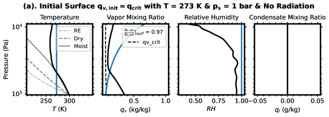
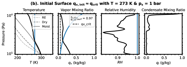
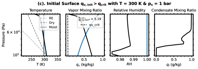
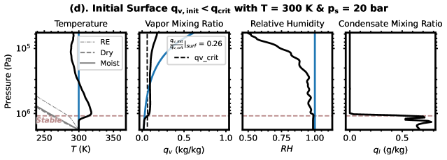
Figure 1: Each row shows the initial (blue) and final (black) atmospheric state from one of the four initially isothermal simulations. In each row, the panels show from left to right, profiles of temperature (K), vapor mixing ratio (kg/kg), relative humidity and condensate mixing ratio (g/kg). In the temperature panels, the gray dashed and solid lines plot a dry and moist adiabats, and the gray dot-dashed line plots the temperature profile assuming gray gas pure radiative equilibrium. The dashed gray line in the vapor mixing ratio panels plots the critical vapor mixing ratio of the final state. In the third row, the final state in the temperature profile lies perfectly on top of the gray moist adiabat curve throughout the domain. The ratio $q_{v,\rm init}/{q_{v,\rm crit}}$ is calculated using the surface values of the initial state of the respective simulation. No initial state is shown in the $q_{l}$ panels as this was set to be zero everywhere in all the simulations.

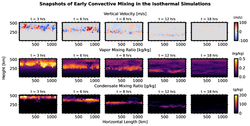
Figure 2: Snapshots of vertical velocity (top row), vapor mixing ratio (middle row), and condensate mixing ratio (bottom row) during the early rapid convective mixing phase in the isothermal simulations. All four isothermal simulations undergo a similar rapid convective mixing phase within the first 12-15 hours. Here, we present the early mixing of the $q_{v,s}~{}<~{}q_{\rm crit}$ test case. Mixing initiates near the top of the domain, driven by dense parcels sinking. Within the convecting layer, as compensating rising air parcels become supersaturated, water vapor condenses within them. The condensate then falls through lower cells and re-evaporates in sub-saturated grid cells. The convecting layer moves down through the atmosphere until it reaches the surface or a neutrally stable layer. In the isothermal simulation initialized with $q_{v,s}~{}<~{}q_{\rm crit}$ (shown here), the convecting layer stops and stabilizes at the top of the Guillot stable region rather than reaching the surface as in the other three isothermal simulations. After the initial rapid mixing, the isothermal simulations reach a convectively stable state, which is subsequently altered on a much slower timescale by radiative processes.

Fig. 1 shows the results from the four isothermal CM1 simulations in each respective row. In each row, the figure shows profiles of (from left to right) temperature (K), vapor mixing ratio (kg/kg), relative humidity and condensate mixing ratio (g/kg). In the first three panels, the blue line shows the initial state of the simulation and the black line shows the final state. In the temperature panel, the gray dot-dashed line plots a temperature profile calculated in pure radiative equilibrium, the gray dashed line is the dry adiabat defined by Eqn. 13, and the gray solid line plots a moist adiabat defined by Eqn. 7. Pure radiative equilibrium is calculated assuming a gray gas atmosphere using,

$$\frac{d\ln{T_{\rm RE}}}{d\ln{p}}=-\frac{1}{4}\frac{1}{(1+\tau_{\infty}-\tau)}p\frac{d\tau}{dp},$$ (15)

where $\tau$ is optical depth, and $\tau_{\infty}$ is the total optical depth of the atmosphere (see Chap.4 Pierrehumbert, 2010). The optical depth is related to the atmospheric opacity by $\frac{d\tau}{dp}~{}=~{}-\frac{1}{2g}~{}\kappa(p)$ where the opacity is determined using Eqn. 12 with the final state CM1 vapor mixing ratio profile. In the vapor mixing ratio panel, the black dashed line plots the critical vapor mixing ratio calculated using Eqn. 11 of the final atmospheric state. The pressure, temperature, and vapor mixing ratio values are calculated by taking the horizontal average of the CM1 data at the given time step. The relative humidity is calculated using the 3D temperature, pressure and vapor mixing ratio outputs from CM1, and the horizontal average of the relative humidity is shown.

First, consider the isothermal test cases where the initial state $p_{s}$ = 1 bar, $T(p)$ = 273 K and the surface $q_{v,\rm sat}\approx q_{\rm crit}$. In Fig. 1, panel (a) shows the atmospheric state without the effects of radiation, while panel (b) shows the atmospheric state with radiation considered. Comparing these two rows, we find that the vapor mixing ratio state is similar. However, there are notable differences in the upper domain atmospheric temperature and relative humidity.

When there are no radiative effects, panel (a) in Fig. 1, the temperature follows a moist adiabat from the surface up until a point in the upper atmosphere where the temperature starts to increase and becomes more isothermal. The region of the atmosphere described by the moist adiabat corresponds to a relative humidity near saturation. In the upper part of the atmosphere, the relative humidity shows the atmosphere is sub-saturated. The temperature profile’s shape in the upper atmosphere is similar to the observed shape of the temperature profile of non-condensing compositional convection simulations in Habib & Pierrehumbert (2024).

Convection is initially driven by compositionally dense air sinking from the top of the domain and heating the atmosphere adiabatically until the parcels reach the surface and can no longer sink. Simultaneously, compensating light air parcels rise and cool the atmosphere adiabatically relative to the initial state. Since the initial state was saturated, as the air parcels rise, they become supersaturated, leading to condensation and latent heat release. This process slightly warms the atmosphere, enhances mixing, and explains why the observed cooling in the upper atmosphere is not as strong as in the dry compositional convection results presented by Habib & Pierrehumbert (2024). Condensates, formed with $q_{l}~{}>~{}1$ g/kg, fall through the lower atmosphere and re-evaporate in sub-saturated grid cells, maintaining saturation in the lower atmosphere. Mixing in the lower atmosphere adjusts the temperature profile to a moist adiabat.

Panel (a) in Fig. 1 shows the atmospheric state after the initial rapid convective mixing, as the temperature profile remains unchanged in simulations without radiation. Additionally, there is no liquid condensate observed in the final state in panel (a), indicating that all condensate formed during the initial rapid mixing phase re-evaporated before a stable state was reached. In the $q_{v,\rm sat}\approx q_{\rm crit}$ simulation without radiation, we find that the system rapidly adjusted due to convective mixing and a final equilibrium state that is convectively stable is reached. Fig. 2 shows snapshots of the vertical velocity, vapor mixing ratio and condensate mixing ratio taken at five time steps early-on within the isothermal simulations to show how mixing occurs during the initial rapid convective adjustment phase. All four isothermal simulations experienced a similar initial rapid adjustment phase that lasted about 12-15 hours.

In the $q_{v,\rm sat}\approx q_{\rm crit}$ simulation with radiation, shown in panel (b) of Fig. 1, we find the lower atmospheric temperature profile still follows a moist adiabat. However, the upper atmospheric temperature profile is cooling due to radiation, as it relaxes towards a radiative equilibrium stratosphere. The radiative cooling in the upper atmosphere leads to condensate formation in the upper domain after the initial rapid convective mixing phase. Note, the relative humidity in $q_{v,\rm sat}\approx q_{\rm crit}$ case with radiation remains near saturation within the entire domain. The final state for the $q_{v,\rm sat}\approx q_{\rm crit}$ simulation with radiation is convectively stable, with both the compositional and temperature profile stable to convection. However, the CM1 final state presented here is not in equilibrium as radiative cooling would continue to modify the atmospheric temperature.

Panel (c) in Fig. 1 shows the atmospheric state for isothermal test case initialized with $p_{s}$ = 1 bar and $T(p)=300$ K, where $q_{v,s}>q_{\rm crit}$. The final atmospheric temperature profile aligns closely with a moist adiabat, with the entire domain near saturation. The alignment is so perfect that the moist adiabat curve is not visible in the temperature profile plot in panel (c). Note that for this case, the moist adiabat in a hydrogen atmosphere is itself quite close to being isothermal. The results for $q_{v,s}>q_{\rm crit}$ are similar to those where $q_{v,\rm sat}\approx q_{\rm crit}$ with radiation, but in the $q_{v,s}>q_{\rm crit}$ case, the initial rapid convective mixing is more vigorous, causing the entire domain’s temperature profile to evolve to a moist adiabat. As before, after the initial mixing, condensation occurs due to radiative cooling in the upper atmosphere, forming a cloud deck in the upper domain. Overall, the system reaches a convectively stable state where both the temperature and compositional profile are stable to convection by the Guillot criterion.

In the preceding cases, the Guillot criterion states that superadiabatic profiles – steeper than the moist adiabat – are stable. Given the optical thickness of the atmosphere, radiation would eventually cause the temperature profile to continue to steepen, towards the radiative equilibrium profiles indicated in the figures. However, for optically thick atmospheres the radiative relaxation time is very long, and the steepening has not yet had time to take place to any significant extent in these simulations. The simulations provide some insight into the basic nature of radiative-convective dynamics in the compositionally-stabilized regime, with the sequence consisting of a rapid adjustment to the moist adiabat followed by a much slower radiative steepening. The steepening effect will be addressed in simulations to be discussed in the following sections.

Panel (d) in Fig. 1 shows the final isothermal CM1 test case initialized with $T=300$ K $p_{s}$ = 20 bar, and $q_{v,s}~{}<~{}q_{\rm crit}$. In this case, the initial state lower atmosphere is stable to moist convection by the Guillot criterion but the entire atmosphere is unstable to dry convection by the Ledoux criterion. Panel (d) in Fig. 1 shows a brown horizontal line dividing the initial Guillot unstable and stable regions within the atmosphere. Interestingly, no convective mixing is observed in the stable region, leaving the final state of this portion of the vertical domain in a saturated isothermal state. The upper atmosphere undergoes an initial rapid mixing phase like the preceding three isothermal simulations. However, in the $q_{v,s}~{}<~{}q_{\rm crit}$ case, sinking air parcels stop just below the stable boundary, and no air parcels are observed rising from the stable region. The temperature profile in the upper atmosphere follows a similar trend to the preceding isothermal simulations. Subsequent radiative cooling steepened the temperature profile in the upper atmosphere and led to a cloud deck forming in the upper atmosphere.

Unlike the previous cases, in the $q_{v,s}~{}<~{}q_{\rm crit}$ case condensing compositional convection is stabilizing the lower domain in the initial atmospheric state. We find that moist compositional stabilization is strong enough to prevent convective mixing in the lower domain. In the final atmospheric state, the temperature and compositional profiles are stable against convection throughout the atmosphere. In the lower domain, the compositional profile increases with height and is unstable according to the Ledoux criterion, but it is stabilized by condensing compositional convection as described by the Guillot criterion. In the $q_{v,s}~{}<~{}q_{\rm crit}$ case, the system mixed only the unstable areas of the domain to the first convectively stable state, with radiative cooling gradually altering this profile over time.

4.2 CM1 Results of the Initially Adiabatic & Superadiabatic Simulations

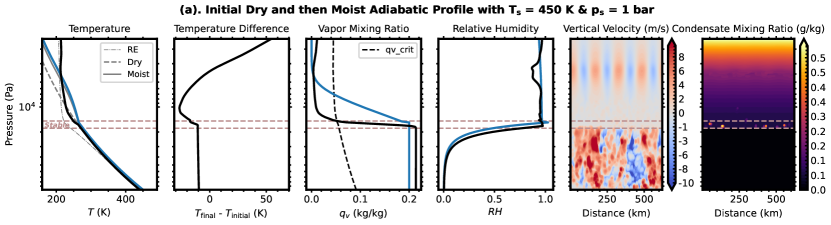
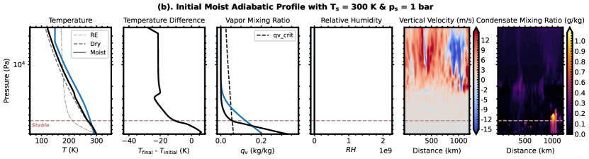
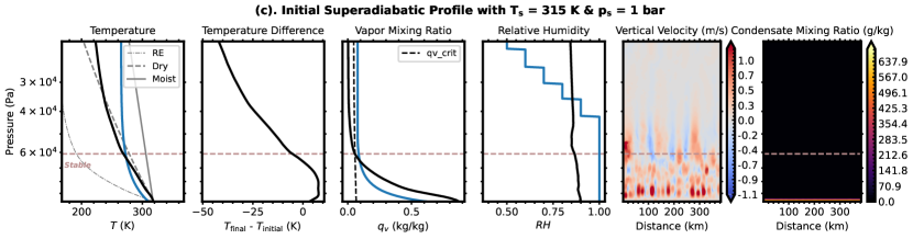
Figure 3: Atmospheric state for the CM1 simulations initialized on (a.) the dry then moist adiabat, (b.) the moist adiabat, and (c.) the superadiabatic state. In each row, the panels show from left to right, profiles of temperature (K), temperature difference between the final and initial state (K), vapor mixing ratio (kg/kg), relative humidity, and vertical cross-sections taken in the middle of the y-domain of vertical velocity (m/s) and condensate mixing ratio (g/kg). In the temperature panels, the gray dashed and solid lines plot a dry and moist adiabats, and the gray dot-dashed line plots the gray gas pure radiative equilibrium temperature profile. The dashed gray line in the vapor mixing ratio panels indicates the critical vapor mixing ratio of the final state. Initial states are illustrated by blue lines in the profile plots, whereas the final state from the CM1 simulation is depicted by the solid black line. The cross-sections are shown for the final state. In panels (a) and (b), we observe only the initial stages of steeping towards a pure radiative equilibrium superadiabatic state, as highlighted in the temperature difference profiles. The simulations show long radiative timescales and the results presented here are not in a statistical equilibrium state.

Fig. 3 shows an overview of the atmospheric state for the CM1 simulations initialized on the (a.) dry then moist adiabat, (b.) moist adiabat, and (c.) superadiabatic profile. Each row shows panels that display, from left to right, vertical profiles of temperature (K), temperature difference between the final and initial state (K), vapor mixing ratio (kg/kg), relative humidity, and 2D cross-sections taken in the middle of the y-domain of the vertical velocity (m/s) and condensate mixing ratio (g/kg). Blue lines indicates the initial state of the CM1 simulation and the black line depict the final state. The 2D cross-sections are shown for the final state. $T(p)$ and $q_{v}(p)$, are determined by taking the horizontal average of the 3D CM1 output at the given timestep. The relative humidity is calculated from the 3D CM1 outputs for $T$, $p$ and $q_{v}$ and its horizontal average is displayed. Brown dashed horizontal lines are used to highlight boundaries between convective and stable atmospheric regions. The three adiabatic test cases were designed such that moist convection is inhibited according to the Guillot criterion within a region of the atmosphere where $q_{v}>q_{\rm crit}$. In the simulations initialized with a moist adiabat and a superadiabatic profile, shown by panel (b.) and (c.) in Fig. 3 respectively, the region stable against moist convection lies below the brown dashed line. While in the dry then moist adiabatic simulation, shown by panel (a.) in Fig. 3, the region where convection is inhibited is located in between the two brown dashed lines.

The CM1 test case initialized on a moist adiabat represents a continuation of the isothermal cases, which generally showed rapid mixing that led to the formation of a convectively stable state, characterized by a moist adiabat in three of the four simulations. The test case starting with a dry then moist adiabat reflects a more realistic scenario where the atmosphere has a deep dry convection zone below an upper moist convecting layer. In the two adiabatic simulations, we found long radiative relaxation timescales, therefore, we performed a CM1 test case initialized on a superadiabatic profile with $q_{v}>q_{\rm crit}$ which is stable to convection according to the Guillot criterion to determine whether saturated, superadiabatic states remain stable over time.

All three simulations presented in Fig. 3 show condensation-driven convective inhibition. The vertical velocity panel for the moist adiabat simulation, middle row of Fig. 3, clearly shows vertical mixing is near zero from the surface up to pressure of $\sim 2x10^{4}$ Pa. Similarly, we observe near zero vertical velocities in the stable region (between the two brown lines) of the dry then moist adiabatic test case and within the whole domain of the superadiabatic simulation. The relative humidity stays near saturation in regions that are convectively stable across all three simulations in Fig. 3. Further, water vapor is transported from the upper to the lower atmosphere from the initial to final state in all three simulations. Superadiabatic temperature profiles begin to form in both the top and middle rows, but neither simulation reaches statistical equilibrium. The CM1 test case initialized on a superadiabatic profile confirms that saturated superadiabatic states where $q_{v}>q_{\rm crit}$ are convectively stable according to the Guillot criterion.

4.2.1 Case I: Simulation Initialized on Dry then Moist Adiabatic Profile

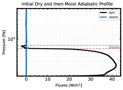
Figure 4: Sensible and latent heat fluxes for the CM1 test case initialized on a dry then moist adiabat. The sensible flux is defined by $Q_{dyn}=C_{p}\langle\rho w^{\prime}\theta^{\prime}\rangle$ and is calculated using the vertical velocity and potential temperature perturbations from CM1. The latent heat flux is $Q_{latent}=L_{v}\langle\rho w^{\prime}q_{v}^{\prime}\rangle$ and is calculated using the vertical velocity and vapor mixing ratio perturbations from CM1. The strong decrease of dynamic heat flux shows convection is strongly suppressed in the stable region. Re-evaporation at the lower boundary of the stable region and dry convection zone leads causes the observed spike in latent heat flux.

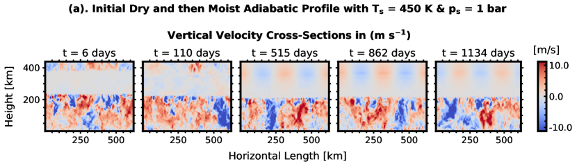
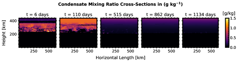
Figure 5: Vertical velocity and condensate cross-sections in (x,z) taken in the middle of the y-domain from adiabatic simulation initialized on the dry adiabat to the level of saturation from which point the initial state followed a moist adiabat. The top row shows the vertical velocity in (m/s) at different times throughout the CM1 simulation. The bottom row shows the condensate mixing ratio in (g/kg) at different times throughout the CM1 simulation. The vertical velocity cross-sections initially show 3 distinct layers; a dry convective region near the surface, a layer where convection is completely inhibited and velocities are nearly zero, and a layer of moist convection in the upper atmosphere. The corresponding condensate mixing ratio plots show a cloud deck from in the moist convection layer and we observe condensates falling through and re-evaporating in the region where convection is completely inhibited.

Figure 6: Eddy diffusivity (left panel) and vertical velocities (right panel) of the CM1 simulation initialized on a dry then moist adaibat. In the left panel, the eddy diffusivity from the CM1 TKE scheme is shown in green, the $K_{zz}$ calculated using Eqn. 16 and is shown in black, and in blue the eddy diffusivity from Leconte et al. (2024) is shown. In the right panel, the RMS velocity, maximum upward and maximum downward velocity from the CM1 simulation is shown in black solid, dashed and dotted lines respectively. The RMS velocity profile from Leconte et al. (2024) is shown in blue for comparison. As before, the brown dashed lines mark the convectively stable region. Note, the Leconte et al. (2024) profile is shifted upwards such that the convective inhibition layer in their result lies within the brown dashed lines.

Consider the CM1 simulation initialized on the dry then moist adiabat as shown in row (a.) of Fig. 3. In this simulation, the deep atmosphere approaches radiative equilibrium, as expected in regions with constant opacity and without pressure broadening. The deep atmosphere is located in a dry convection zone where both the vapor mixing ratio and opacity remain unchanged in our model setup. The thermal structure of the lower atmosphere is largely unchanged from the initial to the final states. A superadiabatic temperature structure begins to form in the stable region in between the two brown lines. Similar, in the upper atmosphere, the temperature profile evolves towards a radiative profile as water vapor is transported to the dry convection zone. The water vapor mixing ratio sharply decreases in the convectively stable region, indicating reduced mixing, similar to findings in Leconte et al. (2024).

Cloud condensate, with $q_{l}(p)<1$ g/kg, forms early in the simulation within the moist convective area. Precipitation develops in the convectively stable region and re-evaporates at the boundary between the stable layer and the dry convection zone. Re-evaporation at this boundary transports moisture to and triggers convective downdrafts in the dry convection area. The re-evaporation level defines the lower boundary between the stable and convecting regions. This is further seen through the latent and sensible heat fluxes in Fig. 4, which shows a sharp spike in the latent heat flux in the convectively stable region corresponding to re-evaporation. The dynamic flux in Fig. 4 shows a sharp decline in the stable region, further supporting that mixing is suppressed within the stable layer. Fig. 4 suggests that some energy is transported through the convective inhibition layer through the latent heat flux, but it does not strongly dominate over the sensible heat flux. This observation differs with the findings in Leconte et al. (2024) where it was noted that in the convective inhibition region, the latent heat flux (about 20 W/m²) dominated over the sensible heat flux, suggesting that energy is carried upward by vapor. In contrast, we find a latent heat flux of about 2 W/m², an order of magnitude smaller than reported by Leconte et al. (2024). A potential source for the difference in the magnitude of latent heat flux between this work and Leconte et al. (2024) could be attributed to variations in model parameterization for condensation. Leconte et al. (2024) employed a condensation scheme where re-evaporation occurs as droplets reach the boiling level. Additionally, their scheme does not differentiate between cloud and rain condensates, unlike our approach.

We present a time evolution of 2D cross-sections taken in the middle of the y-domain, showing vertical velocities (m/s) and corresponding condensate mixing ratio (g/kg) for the dry then moist adiabatic simulation in Fig. 5. Initially, Fig. 5 shows a distinct region where vertical mixing is suppressed separating an upper moist convection zone from a lower dry convection zone. As the simulation progresses, vertical velocities in the moist convective zone weaken due to the transport of water vapor to the dry convection zone. Eventually, the weak convection cells form in the upper atmosphere where the vertical velocities are small but still greater than the convectively inhibited area.

Unlike the findings in Leconte et al. (2017), our results indicate that diffusive fluxes are insufficient to transport enough water vapor upwards from the stable region to sustain strong moist convection. We further illustrate this in Fig. 6 which shows the eddy diffusivity flux in left panel and the RMS vertical velocity profile in right panel. Following Leconte et al. (2024), the resolved eddy diffusivity, $K_{zz}$ is defined as

$$K_{zz}^{EddyFlux}=\frac{\langle\rho q_{v}w\rangle}{\rho\langle\frac{dq_{v}}{dz}\rangle},$$ (16)

where $\rho$ is the total density, $q_{v}$ is the vapor mixing ratio, $w$ is the vertical velocity, $z$ is height, and $\langle\rangle$ denote spatial and temporal averages. In Fig. 6 the eddy diffusivity of the dry then moist adiabatic simulation in plotted in black with $K_{zz}$ profile from Leconte et al. (2024) shown in blue for comparison. Additionally, we plot a green line showing the parameterized sub-grid eddy diffusivity output from CM1. CM1 uses the TKE sub-grid turbulence parameterization (Deardorff, 1980) which uses a predictive turbulent kinetic energy to determine an eddy viscosity and diffusivity to represent mixing on sub-grid scales. The TKE scheme has a stability dependence that reduces sub-grid mixing in statically stable conditions. The vertical velocity panel in Fig. 6 shows the RMS velocity, the maximum upward and downward velocities in black solid, dashed and dotted lines, respectively. The RMS velocity profile from Leconte et al. (2024) is shown in blue for comparison and the sub-grid velocity from the TKE scheme is shown in green. Note that the profiles from Leconte et al. (2024) are shifted upwards so that the stable regions of the two studies align for easier comparison.

Our model shows similar profile shape and magnitude RMS vertical velocity and $K_{zz}$ in the lower atmosphere and convective inhibition layer compared to findings in Leconte et al. (2024). Interestingly, we observe that both $K_{zz}$ and the RMS vertical velocity remain comparable to the stable convective inhibition region slightly above the upper boundary of the stable region. This may indicate a transition or boundary layer where convection still seems to be suppressed even though $q_{v}(p)<q_{crit}$. The upper boundary of the stable region is defined by $q_{v}(p)=q_{crit}$, beyond which the Guillot criterion no longer predicts convective inhibition. A transition or boundary region was not found in the results presented by Leconte et al. (2024). $K_{zz}$ and the vertical velocity increases in the moist convection region immediately above the stable layer in the results from Leconte et al. (2024) compared to this work.

In general, the $K_{zz}$ and the vertical velocity profiles suggest that convection is still suppressed above the stable layer within the CM1 results, supporting earlier observations that moist convection is weakening in the upper atmosphere. We attribute the difference in mixing magnitude above the stable layer between this work and Leconte et al. (2024) to variations in model setup, particularly in the condensation and turbulence parameterizations. Leconte et al. (2024) used a different condensation scheme and found an order of magnitude higher latent heat flux in the stable layer, which could enhance mixing in their model’s upper atmosphere. Additionally, we employ a sub-grid turbulence parameterization, whereas Leconte et al. (2024) did not. In the TKE sub-grid parameterization used in CM1, mixing is suppressed in statically stable regions, which could further reduce mixing in the upper atmosphere in our CM1 simulation results. Due to the lower eddy diffusivity and vertical velocities in our model results, we do not transport enough water vapor upwards to sustain strong moist convection in the upper atmosphere unlike Leconte et al. (2024).

Overall the dry then moist adiabatic simulation shows that the compositional gradient can suppress convection. Despite the clear formation of a convective inhibition layer, we do not observe the temperature profile to adjust to a steep radiative profile. Our simulations indicate that the timescale for convection to adjust the atmospheric state profile is relatively fast, as shown by the isothermal initialization cases. However, the radiative processes are slow. Since the simulations confirm that convection is inhibited, radiative relaxation should eventually proceed to produce steep radiative layers. In Section 4.3 we discuss that the relaxation time is too long for steep radiative layers to form within the duration of the CM1 simulations.

4.2.2 Case II: Simulation Initialized on a Moist Adiabatic Profile

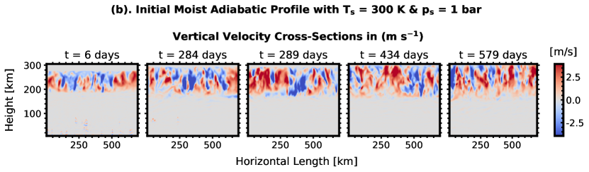
Figure 7: Vertical velocity and condensate cross-sections in (x,z) taken in the middle of the y-domain for the adiabatic simulation initialized on the moist adiabat. The top row shows the vertical velocity in [m/s] at different times throughout the CM1 simulation. The bottom row shows the condensate mixing ratio in [g/kg] at different times throughout the CM1 simulation. The vertical velocity cross-sections show clear convective inhibition in the lower atmosphere in all time steps. The corresponding condensate mixing ratio show a condensate formation nearly in the whole domain, but re-evaporation occurs at the boundary between the stable and convection regions.

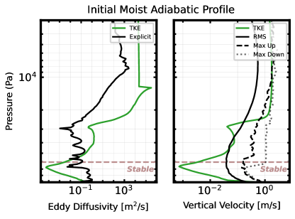
Figure 8: Eddy diffusivity (left panel) and vertical velocities (right panel) of the CM1 simulation initialized on a moist adaibat. In the left panel, the eddy diffusivity from the CM1 test case is calculated using Eqn. 16. In the right panel, the RMS velocity, maximum upward and maximum downward velocity from the CM1 simulation is shown in black, solid, dashed and dotted lines respectively. The green line plots the eddy diffusivity and vertical velocity output from the CM1 sub-grid turbulence parameterization. As before, the brown dashed lines mark the convectively stable region.

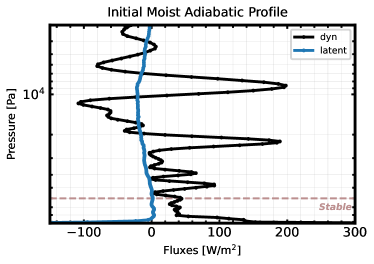
Figure 9: Sensible and latent heat fluxes for the CM1 test case initialized on a moist adiabat. The sensible flux is defined by $Q_{dyn}=C_{p}\langle\rho w^{\prime}\theta^{\prime}\rangle$ and is calculated using the vertical velocity and potential temperature perturbations from CM1. The latent heat flux is $Q_{latent}=L_{v}\langle\rho w^{\prime}q_{v}^{\prime}\rangle$ and is calculated using the vertical velocity and vapor mixing ratio perturbations from CM1.

In the CM1 simulation initialized on a moist adiabat, shown in panel (b.) of Fig. 3, the thermal profile in the upper convecting atmosphere lies between a dry and moist adiabat, while the stable region’s thermal profile is steepening over time. As in the previous case, the stable region seems to extend beyond where the Guillot criterion predicts compositional driven convective inhibition (brown line) to a pressure of about $2\times 10^{4}$ Pa. The temperature profile is steepening from the surface up to $2\times 10^{4}$ Pa, and evolving towards a radiative profile. Within the stable region, moisture is transported to the lower atmosphere towards the surface.

Fig.7 shows vertical velocity and condensate mixing ratio cross-sections for the CM1 simulation initialized on a moist adiabat. Convection is noticeably inhibited in the lower atmosphere, with suppressed vertical velocity extending above the upper boundary of the stable region to a pressure of about $2\times 10^{4}$ Pa (approximately 200 km above the surface). Unlike the previous case, the convective velocities in the upper atmosphere remain of a similar order of magnitude throughout the simulation, and we do not observe a significant weakening of moist convection in this case. Fig.8 shows the $K_{zz}$ (left) and RMS vertical velocity (right) profiles. The black line shows the $K_{zz}$ calculated using Eqn. 16 and RMS vertical velocity, while the green line plots the $K_{zz}$ and vertical velocity from CM1’s TKE sub-grid turbulence scheme, respectively. The explicit $K_{zz}$ (left) and RMS vertical velocity (right) profile in Fig.8 confirms that vertical velocities and eddy diffusivity remain suppressed throughout and beyond the inhibited layer up to about $2\times 10^{4}$ Pa, where they then begin to increase. However, sub-grid mixing increases above the brown line indicating where Guillot criterion predicts convective inhibition, suggesting mixing is not inhibited above the brown line but rather remains suppressed. As in the dry then moist adiabatic case, $K_{zz}$ and both the 1D (Fig.8) and 2D (Fig.7) velocity plots suggest that mixing seems to remain suppressed above where the Guillot criterion predicts the boundary of the stable region indicating the presence of a transition or boundary layer above the convective inhibition region.

Fig. 9 shows the dynamic and latent heat fluxes for the moist adiabatic test case. The latent heat flux is approximately -20 $\rm W/m^{2}$ in the moist convective region of the upper atmosphere due to condensation and re-evaporation, remains small in the stable region, but peaks again at the surface due to condensation and re-evaporation. The latent heat flux contributes to energy transport primarily in the moist convective region. The dynamic heat flux is constant and near zero in the stable region, supporting convective inhibition in the stable layer, but oscillates in the convective region due to small-scale mixing in the upper atmosphere. The dynamic flux remains small but does increase immediately above the stable layer supporting the argument for a boundary layer above the stable region.

As in the previous simulation, we do not observe the temperature profile adjusting to a steep radiative profile, again indicating that radiative processes are slow. Since the simulations confirm that convection is inhibited, radiative relaxation should eventually proceed to produce steep radiative layers.

4.2.3 Case III: Simulation Initialized on a Superadiabatic Profile

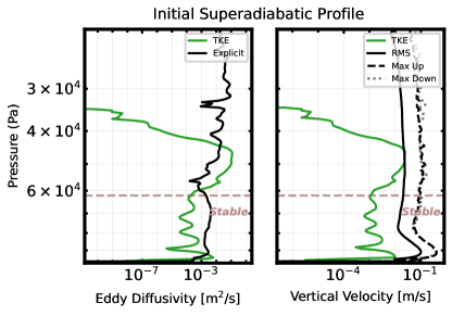
Figure 10: Eddy diffusivity (left panel) and vertical velocities (right panel) of the CM1 simulation initialized on a superadiabatic profile. In the left panel, the eddy diffusivity from the CM1 test case is calculated using Eqn. 16 and shown by the black line. In the left panel, the RMS velocity, maximum upward and maximum downward velocity from the CM1 simulation is shown in black, sold, dashed and dotted lines respectively. The green line plots the eddy diffusivity and vertical velocity output from the CM1 sub-grid turbulence parameterization. The brown dashed lines marks the convectively stable region.

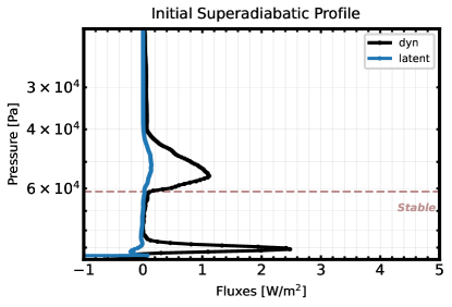
Figure 11: Sensible and latent heat fluxes for the CM1 test case initialized on a superadiabatic profile. The sensible flux is defined by $Q_{dyn}=C_{p}\langle\rho w^{\prime}\theta^{\prime}\rangle$ and is calculated using the vertical velocity and potential temperature perturbations from CM1. The latent heat flux is $Q_{latent}=L_{v}\langle\rho w^{\prime}q_{v}^{\prime}\rangle$ and is calculated using the vertical velocity and vapor mixing ratio perturbations from CM1.

The CM1 simulation initialized on a superadiabatic profile shows no convective mixing or significant vertical velocities throughout the entire simulation. Fig. 3 shows the temperature profile is steepening due to radiation. As in previous cases, moisture is transported from the upper to lower atmosphere through condensation and rain fallout. Vertical velocities are minimal and primarily driven by falling condensates. The entire domain remains near saturation, with re-evaporation occurring at the upper boundary of the stable layer. Fig. 10 shows that the eddy diffusivity is 1–2 orders of magnitude lower in the stable region compared to the rest of the domain. Notably, the eddy diffusivity is around $10^{-3},\rm m^{2}/s$ within the condensation-driven inhibition region, about $10^{-2},\rm m^{2}/s$ just above the stable layer, and approximately $10^{-1},\rm m^{2}/s$ in the upper atmosphere. The superadiabatic case clearly shows convection is inhibited when $q_{v}(p)>q_{\rm v,crit}(p)$, and a transition boundary layer forms above the stable region where velocities remain small. Lastly, Fig. 11 shows that both the dynamic and latent heat fluxes are a couple orders of magnitude smaller than in preceding cases, with peaks only in regions of condensation and re-evaporation. As with previous cases, the superadiabatic simulation has not yet reached radiative equilibrium, and the timescale for this process is discussed in the next section.

4.3 Evaluating CM1 Radiative Timescales & Convergence

Table 3: Estimation of radiative timescale from diffusive gray gas estimation given by Eqn. 17, and a time-stepping method that iteratively solves the gray gas radiative transfer equations.

	Diffusive	Time-stepping
	[yrs.]	[yrs.]
Initial Isothermal Simulations
Isothermal $q_{v}<q_{\rm crit}$	2	4
Isothermal $q_{v}\approx q_{\rm crit}$	1	4
Isothermal $q_{v}>q_{\rm crit}$	1	1
Initial Adiabatic Simulations
Dry then Moist Adiabat	1	4
Moist Adiabat	1	5
Superadiabatic	1	3

The radiative relaxation timescale for the CM1 simulations presented in this work is relatively long, preventing the simulations from converging to a statistical equilibrium state. We find in the CM1 simulations that the temperature tendency is on the order of $10^{-5}-10^{-7}~{}K~{}s^{-1}$, highlighting the extended duration of the radiative relaxation timescale across all simulations. To quantify the radiative timescale, we estimate the diffusive radiative timescale required to reach gray gas radiative equilibrium, defined as

$$\tau_{\text{rad}}\sim\frac{P}{g}\frac{C_{p}}{4\sigma T^{3}}$$ (17)

where $C_{p}$ is the heat capacity, $\kappa$ is the opacity, and $\sigma$ is the Stefan-Boltzmann constant (Showman & Guillot, 2002). Additionally, we estimate the radiative timescale by time-stepping the final CM1 profile to a state of radiative equilibrium where $I_{+}-I_{-}$ is constant with height. To determine the temperature profile in radiative equilibrium, we begin with the final CM1 profile and determine the upward and downward radiative fluxes and temperature tendency using the gray gas Schwarzschild equations. We then heat or cool the CM1 profile by,

$$T(p,t+1)=T(p,t)+\frac{dT}{dt}\cdot dt,$$ (18)

where $T(p,t+1)$ is the new temperature profile, $\frac{dT}{dt}$ is the calculated temperature tendency, and $dt$ is the time step. The new temperature profile is used to update the temperature tendency using the gray gas radiative transfer equations. This calculation is iterated until the heating rate, $\frac{dT}{dt}$, is two orders of magnitude smaller than the observed heating rate in the final state of the CM1 output. This approach offers a method to estimate the radiative relaxation time. However, it assumes that the atmosphere is entirely non-convective and neglects the interactions between convective and inhibited regions. Therefore, this calculation should be viewed as an indication of the time required for the inhibited regions to reach equilibrium. Table 3 provides the estimated radiative timescale from the two methods for all six of the CM1 simulations involving radiation. Note, that the time-stepping method provides a indication of the additional time it would take to run the CM1 simulation until the temperature tendency is two orders of magnitude less than the current final state output from CM1. Additionally, the radiative fluxes and temperature tendencies for the final CM1 state are provided in the Appendix for each simulation.

The CM1 simulation results have not yet achieved a state of statistical equilibrium, indicating that radiation could still influence the temperature profile, albeit over long timescales. The CM1 adiabatic simulations reveal the formation of convectively inhibited layers and begin to show steepening of the temperature profile in stable regions, but they have not reached a quasi-equilibrium state or developed steep radiative temperature profiles.

5 Conclusions

In this work, we use 3D convection-resolving simulations to explore compositional-driven convective inhibition in H₂-dominated atmospheres. Any atmospheric tracer has a larger mean molecular weight than H₂. Therefore, compositional gradients of tracers in H₂-rich atmospheres have the potential to strongly suppress convection or even inhibit convection if the tracer is condensing and the vapor mixing ratio exceeds a critical threshold, $q_{\rm crit}$ (Guillot, 1995). Previous 1D studies hypothesized that if a condensing tracer inhibited convection in H₂-rich atmospheres, the sole mechanism to transport heat in convectively inhibited layers is radiation. This would result in a radiative superadiabatic temperature profile forming in the stable, inhibited layers (Leconte et al., 2017).

In this work, we use 3D convection-resolving simulations with CM1 to test the hypothesis proposed by (Leconte et al., 2017). We performed two sets of simulations: first, we considered simulations initialized on saturated isothermal states, and second, we considered simulations initialized on adiabatic profiles. The isothermal simulations show that an isothermal temperature profile can be destabilized due to a compositional gradient. These simulations exhibit rapid initial convection that adjusts the atmospheric state to a convectively stable state defined by a moist adiabat when $q_{v}(p)>q_{\rm crit}$.

In the adiabatic CM1 simulations, the initial atmospheric state is convectively stable, but we observe the formation of a distinct layer where convection is inhibited. The convective inhibition layer forms where the atmosphere is saturated and $q_{v}(p)>q_{\rm crit}$. Overall, the adiabatic simulations suggest a tendency towards steepening the temperature profile beyond the adiabatic slope in the stable, convective inhibition layers. Additionally, the adiabatic simulations show the formation of a transition region above the stable layer where velocities and transport of vapor is still small. Vapor is transported from the upper to the lower atmosphere through the re-evaporation of condensates at the boundary of convective and inhibited regions. These simulations also suggest that latent heat flux does transports a small amount of energy through convectively inhibited layers. Due to the transport of vapor from the upper to the lower atmosphere, and the relatively low latent heat flux, we find in our dry then moist adiabatic simulation that moist convection in the upper atmosphere weakens over time. A caveat of this work is that all the simulations have relatively long radiative relaxation times, and the results have not converged to a statistical-equilibrium state. To confirm if saturated, superadiabatic temperature profiles are stable according to the Guillot criterion, we performed a CM1 simulation initialized on a saturated superadiabatic state and found it remains stable against convection over long timescales.

Leconte et al. (2024) conducted a similar 3D convection-resolving simulation to determine if condensation-driven convective layers form in H₂-rich atmospheres and to characterize the resulting atmospheric state. The modeling framework and simulation setup in this work differ from that used in Leconte et al. (2024). Notably, the physics parameterizations in this work and Leconte et al. (2024) vary. Leconte et al. (2024) employed a correlated-k radiation scheme, did not use any sub-grid turbulence schemes, and implemented a condensation scheme where condensation occurs when $q_{v}(p)>q{v,sat}(p)$ and re-evaporation occurs at the boiling point. Generally, both studies find that convection is effectively suppressed in saturated regions where $q_{v}(p)>q_{crit}$ in H₂-dominated atmospheres, and re-evaporation occurs at the boundary of the convectively stable region, allowing latent heat to transport energy to the stable layer. However, in this work, we find that the latent heat flux is an order of magnitude smaller than those reported in Leconte et al. (2024), resulting in weaker water vapor transport into the upper atmosphere and a weakening of the moist convective region. Conversely, Leconte et al. (2024) report that vapor diffuses upwards and sustains strong moist convection in the upper atmosphere.

Our results suggest that condensing tracers can be depleted in the upper atmosphere of planets with H₂-rich atmospheres, potentially preventing these species from being detected in sub-Neptune atmospheres. Moist convection in the upper atmosphere could be restored by a giant storm in which deep convection mixes the troposphere, as proposed by Li & Ingersoll (2015). After a giant storm, the tropospheric temperature profile would reset to an adiabatic state, and radiative cooling would then restart the process of cooling the atmosphere. While this work has focused on water vapor in H₂-rich atmospheres, condensation-driven convective inhibition can occur for any condensing tracer that is heavier than the background atmosphere. Convectively stable layers could potentially form in magma ocean planets due to the gradient of silicates in these planets Markham et al. (2022).

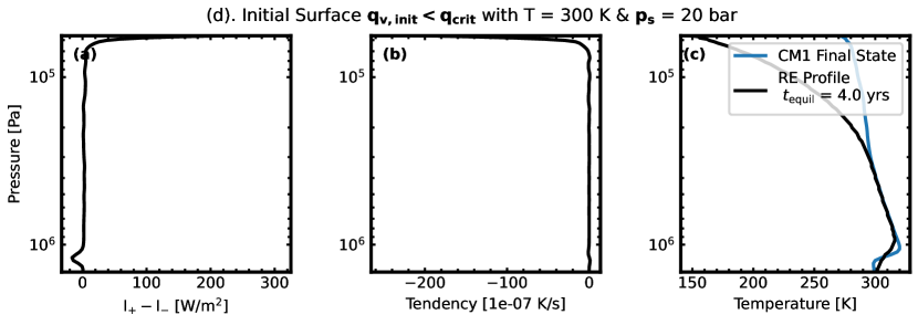
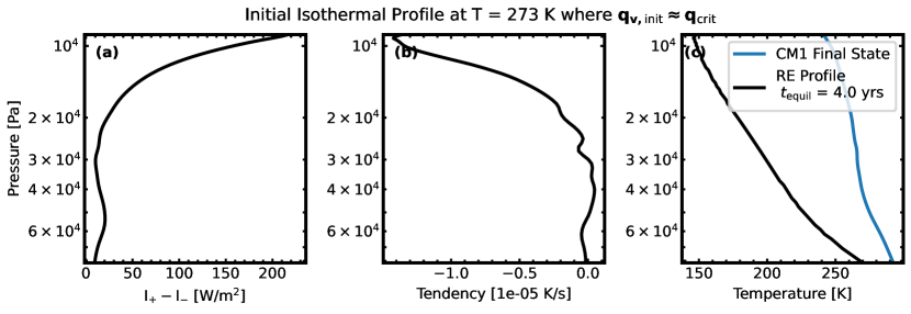
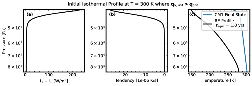
Figure 12: Radiative fluxes for the initially isothermal compositional convection CM1 simulations. Panel (a) shows the difference of the upward and downward longwave infrared flux, $I_{+}-I_{-}$ and panel (b) shows the temperature tendency, $\frac{dT}{dt}$, calculated by the TWOSTR numerical package in CM1. Panel (c) plots the final state CM1 profile in blue and the temperature profile if the CM1 final state is forced to radiative equilibrium (RE) in black.

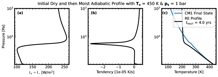
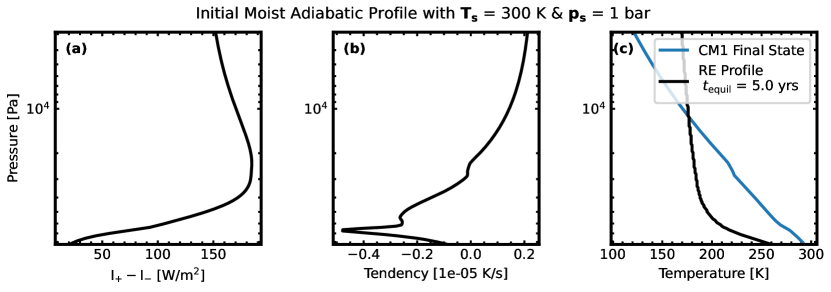
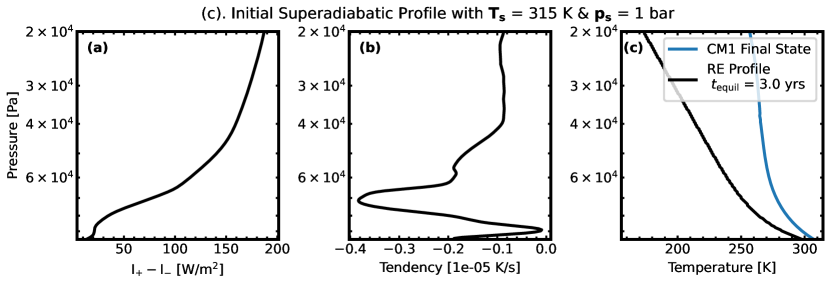
Figure 13: CM1 Radiative fluxes and estimated radiative timescale for initially adiabatic simulations. Panel (a) shows the difference of the upward and downward longwave infrared flux, $I_{+}-I_{-}$ and panel (b) shows the temperature tendency, $\frac{dT}{dt}$, calculated by the TWOSTR numerical package in CM1. Panel (c) plots the final state CM1 profile in blue and the temperature profile if the CM1 final state is forced to radiative equilibrium (RE) in black. The calculated radiative equilibrium profile provides an indication of the radiative relaxation timescale and the temperature for the layer where convection is inhibited.

We show an overview of the radiation fluxes and temperature tendency calculated by the TWOSTR numerical package in CM1 for the isothermal simulations in Fig. 12 and the adiabatic simulations in Fig. 13. In panel (a), we plot the difference of the upward and downward longwave infrared flux, $I_{+}-I_{-}$, and in panel (b) we show the temperature tendency, $\frac{dT}{dt}$. The temperature tendency is defined,

$$\frac{dT}{dt}=\frac{g}{C_{p,{\rm mix}}(p)}\frac{d(I_{+}-I_{-})}{dp},$$ (1)

where $g$ is the gravitational acceleration, $C_{p,{\rm mix}}$ is the heat capacity of the mixture of background and tracer at a given pressure. We find in our CM1 simulations that the temperature tendency is on the order of $10^{-5}-10^{-7}~{}K~{}s^{-1}$, suggesting that the radiative relaxation timescale is quite long in all of our simulations.

To quantify the radiative relaxation time, we utilized the final output profile from CM1 to estimate the time required to reach radiative equilibrium and to determine the corresponding temperature profile assuming convection is inhibited everywhere. In panel (c) of Fig. 12-13, we plot the final temperature state from CM1 in blue, alongside the temperature profile that would result if the system were forced into radiative equilibrium, meaning $I_{+}-I_{-}$ is constant with height. To determine the temperature profile in radiative equilibrium, we time-stepped the final CM1 profile using the calculated temperature tendency as described in Section 4.3. Fig. 13 and Fig. 12 demonstrates that the CM1 simulation results have not yet achieved a state of statistical equilibrium, and that radiation still has the potential to modify the temperature profile, albeit over an extremely long timescales.

References

- Benneke et al. (2024) Benneke, B., Roy, P.-A., Coulombe, L.-P., et al. 2024, JWST Reveals CH$_4$, CO$_2$, and H$_2$O in a Metal-rich Miscible Atmosphere on a Two-Earth-Radius Exoplanet, arXiv, doi: 10.48550/arXiv.2403.03325
- Bryan (2009) Bryan, G. H. 2009, The Governing Equations for Cloud Model 1. http://www.mmm.ucar.edu/people/bryan/cm1/cm1_equations.pdf
- Daley-Yates et al. (2021) Daley-Yates, S., Padioleau, T., Tremblin, P., Kestener, P., & Mancip, M. 2021, Astronomy & Astrophysics, 653, A54
- Deardorff (1980) Deardorff, J. W. 1980, Boundary-layer meteorology, 18, 495
- Emanuel (1994) Emanuel, K. A. 1994, Atmospheric Convection (Oxford University Press, USA)
- Freedman et al. (2014) Freedman, R. S., Lustig-Yaeger, J., Fortney, J. J., et al. 2014, The Astrophysical Journal Supplement Series, 214, 25
- Friedson & Gonzales (2017) Friedson, A. J., & Gonzales, E. J. 2017, Icarus, 297, 160, doi: 10.1016/j.icarus.2017.06.029
- Guillot (1995) Guillot, T. 1995, Science, 269, 1697, doi: 10.1126/science.7569896
- Habib & Pierrehumbert (2024) Habib, N., & Pierrehumbert, R. T. 2024, The Astrophysical Journal, 961, 35, doi: 10.3847/1538-4357/ad04e2
- Innes et al. (2023) Innes, H., Tsai, S.-M., & Pierrehumbert, R. T. 2023, The Astrophysical Journal, 953, 168, doi: 10.3847/1538-4357/ace346
- Irwin et al. (2022) Irwin, P. G. J., Teanby, N. A., Fletcher, L. N., et al. 2022, Journal of Geophysical Research: Planets, 127, e2022JE007189, doi: 10.1029/2022JE007189
- Kylling et al. (1995) Kylling, A., Stamnes, K., & Tsay, S. C. 1995, Journal of Atmospheric Chemistry, 21, 115, doi: 10.1007/BF00696577
- Leconte et al. (2017) Leconte, J., Selsis, F., Hersant, F., & Guillot, T. 2017, Astronomy & Astrophysics, 598, A98
- Leconte et al. (2024) Leconte, J., Spiga, A., Clément, N., et al. 2024, A 3D picture of moist-convection inhibition in hydrogen-rich atmospheres: Implications for K2-18 b, arXiv, doi: 10.48550/arXiv.2401.06608
- Ledoux (1947) Ledoux, P. 1947, Astrophysical Journal, 105, 305
- Lefèvre et al. (2022) Lefèvre, M., Tan, X., Lee, E. K. H., & Pierrehumbert, R. T. 2022, The Astrophysical Journal, 929, 153, doi: 10.3847/1538-4357/ac5e2d
- Li & Ingersoll (2015) Li, C., & Ingersoll, A. P. 2015, Nature Geoscience, 8, 398, doi: 10.1038/ngeo2405
- Luque & Pallé (2022) Luque, R., & Pallé, E. 2022, Science, 377, 1211, doi: 10.1126/science.abl7164
- Madhusudhan et al. (2021) Madhusudhan, N., Piette, A. A. A., & Constantinou, S. 2021, The Astrophysical Journal, 918, 1, doi: 10.3847/1538-4357/abfd9c
- Markham et al. (2022) Markham, S., Stevenson, D., & Guillot, T. 2022, arXiv preprint arXiv:2207.04708
- Menou (2011) Menou, K. 2011, The Astrophysical Journal Letters, 744, L16
- Misener & Schlichting (2022) Misener, W., & Schlichting, H. E. 2022, Monthly Notices of the Royal Astronomical Society, 514, 6025
- Pierrehumbert (2010) Pierrehumbert, R. T. 2010, Principles of Planetary Climate (Cambridge University Press)
- Pierrehumbert (2023) —. 2023, The Astrophysical Journal, 944, 20, doi: 10.3847/1538-4357/acafdf
- Rotunno & Emanuel (1987) Rotunno, R., & Emanuel, K. A. 1987, Journal of Atmospheric Sciences, 44, 542
- Showman & Guillot (2002) Showman, A. P., & Guillot, T. 2002, Astronomy & Astrophysics, 385, 166
- Tan et al. (2021) Tan, X., Lefèvre, M., & Pierrehumbert, R. T. 2021, The Astrophysical Journal Letters, 923, L15
- Van Eylen et al. (2018) Van Eylen, V., Agentoft, C., Lundkvist, M. S., et al. 2018, Monthly Notices of the Royal Astronomical Society, 479, 4786, doi: 10.1093/mnras/sty1783
- Yang & Seidel (2020) Yang, D., & Seidel, S. D. 2020, Journal of Climate, 33, 2841
- Yang et al. (2019) Yang, H., Komacek, T. D., & Abbot, D. S. 2019, arXiv, 876, L27, doi: 10.3847/2041-8213/ab1d60
- Young et al. (2023) Young, E. D., Shahar, A., & Schlichting, H. E. 2023, Nature, 616, 306