Acceleration deforms exponential decays into power laws

Abstract

An exponentially decaying accelerated system looks as if its decay was of a generalized power-law type, provided relativistic time dilation in the detector and retardation of the emitted signal are taken into account. The same mathematical formula is found in generalizations of the Zipf-Mandelbrot law in quantitative linguistics, and in dynamics of re-association of folded proteins.

I Watching a decay

Assume an unstable system propagating along a world-line $r\mapsto x^{\mu}(r)$ in Minkowski space decays exponentially in its own reference frame. The survival probability at proper time $r$ is given by $p(r)=e^{-r/r_{0}}$. Here, $r\geq 0$ is the proper time computed along the world-line and $r_{0}$ is the mean lifetime (we measure proper time in units of length). Now, consider another world-line, $s\mapsto y^{\mu}(s)$, describing a detector which absorbs at $y^{\mu}(s)$ the light signal emitted at $x^{\mu}(r)$. Here, $s\geq 0$ is the proper time of the detector, computed along the detector’s world-line. The difference $y^{\mu}(s)-x^{\mu}(r)$ is a future-pointing null vector. We also assume that at the moment the decay begins, at $r=s=0$, both objects are at the same point in space-time, $x^{\mu}(0)=y^{\mu}(0)$. If the decay takes place at proper time $r$, it will be detected at proper time $s=s(r)$ which depends on both world-lines (Fig. 1).

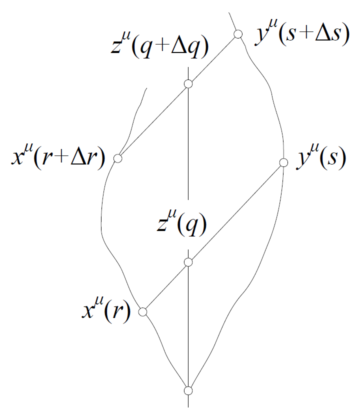
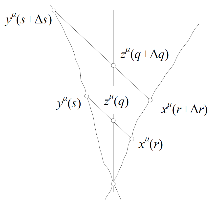
Figure 1: The geometry of the problem. We assume the world lines begin at the same point (the left picture), then cross once again and tend towards their asymptotic forms (the right picture). This type of evolution is typical of sources and detectors that move with opposite accelerations. The world-lines $r\mapsto x^{\mu}(r)$ and $s\mapsto y^{\mu}(s)$ represent, respectively, the source and the detector. The auxiliary world-line $q\mapsto z^{\mu}(q)$ represents the rest frame. The points $x^{\mu}(r)$, $z^{\mu}(q)$, and $y^{\mu}(s)$ are located on the same light cone. The same concerns their versions shifted by $\Delta r$, $\Delta q$, and $\Delta s$. In effect, the three proper-time parameters are not independent of one another. In order to find the explicit form of $s(r)$ it is simplest to split the derivation into two steps, $q(r)$ and $s(q)$.

The problem is nontrivial in that accelerated sources or detectors may lead to event horizons. In particular, a particle that decays exponentially in its rest frame may approach the event horizon of the detector in a finite time $r_{\rm max}$, but the detector will have to wait forever to see the source cross the horizon if $s(r_{\rm max})=\infty$. Accordingly, $P(s)$ cannot be exponential because $P(\infty)\neq 0$.

The probability of non-detection, $P(s)$, equals the probability of non-emission, when signal retardation and time dilation in the detector are taken into account. Hence, we assume

$$P(s(r))=p(r),\quad P(s)=p(r(s)).$$ (1)

The question is what are the forms of $s(r)$, $r(s)$ and $P(s)$?

The observed $P(s)$ cannot be exponential if an event horizon occurs. However, we will show below that $P(s)$ is never exponential when there are accelerations, regardless of the presence or absence of a horizon. We find an explicit closed-form solution for the case of sources and detectors moving with constant (but opposite) accelerations,

$$P(s) = \left\{\begin{array}[]{rl}\left(1-\frac{|a|}{|b|}c^{-2}(U_{0}-|\bm{U}|)(V_{0}-|\bm{V}|)(e^{|b|s/c^{2}}-1)\right)^{\frac{c^{2}}{|a|r_{0}}},&0\leq s\leq s_{1},\\ \left(1+\frac{|a|}{|b|}c^{-2}(U_{0}+|\bm{U}|)(V_{0}+|\bm{V}|)(1-e^{-|b|s/c^{2}})\right)^{-\frac{c^{2}}{|a|r_{0}}},&s\geq s_{1},\end{array}\right.$$ (4)

where $s_{1}=s(r_{1})$ is the value of the detector proper time corresponding to the moment the world-lines cross the second time (that is, if $x^{\mu}(r_{1})=y^{\mu}(s_{1})$ for a nonzero value $r=r_{1}>0$; the first time they cross occurs at the initial condition $r=s=0$). Parameters $a$ and $b$ are the accelerations of the source and the detector, respectively, whereas $U^{\mu}$ and $V^{\mu}$ are their initial world-velocities. For a nonzero detector acceleration, $b\neq 0$, one finds

$$P(\infty) = \left(1+\frac{|a|}{|b|}c^{-2}(U_{0}+|\bm{U}|)(V_{0}+|\bm{V}|)\right)^{-\frac{c^{2}}{|a|r_{0}}}=e^{-r_{\rm max}/r_{0}}\neq 0.$$ (5)

A finite value of $r_{\rm max}$ means that the event horizon occurs for the detector. The limit $b\to 0$ describes a detector that moves with no acceleration,

$$\lim_{b\to 0}P(s) = \left\{\begin{array}[]{rl}\left(1-|a|(U_{0}-|\bm{U}|)(V_{0}-|\bm{V}|)s/c^{3}\right)^{\frac{c^{2}}{|a|r_{0}}},&0\leq s\leq s_{1},\\ \left(1+|a|(U_{0}+|\bm{U}|)(V_{0}+|\bm{V}|)s/c^{3}\right)^{-\frac{c^{2}}{|a|r_{0}}},&s\geq s_{1}.\end{array}\right.$$ (8)

The exponential decay is then replaced by an exact power law, but the event horizon disappears.

The replacement of an exponential law by a power law is a purely relativistic effect. It should not be confused with other possible reasons for deviations from a simple exponential formula one finds in experiment. We know, for example, that the spontaneous emission of an excited atomic state is exponential only approximately, but this is not what we are concerned with here. The formula we derive below will have its analogue for any form of the decay, and the result will be again given by (1). Systems accelerating in more complicated ways will lead to more complicated forms of $s(r)$, still satisfying our differential equation for $ds(r)/dr$. Our derivation is generally valid for any motion of sources and detectors.

Somewhat unexpectedly, the probability given by (4) (especially when written as (75)) turns out to have exactly the form postulated over two decades ago by Tsallis, Bemski and Mendes [1] in their analysis of re-association of folded proteins [2, 3]. Moreover, inspired by [1], Montemurro [4] showed that the same probability function can be used to adequately model observable deviations from the Zipf-Mandelbrot law in quantitative linguistics. All these links with the problem discussed in the present paper were completely unexpected and hard to anticipate. It should be stressed, though, that neither [1] nor [4] were capable of deriving (4) and (75) from first principles — rather, it was an educated guess based on the structure of the data and an ad hoc modification of some differential equations.

A step towards a first-principles derivation of (4) and (75), although completely unrelated to what we discuss in the present paper, was made in [5]. What we showed in [5] was that probabilities of the form (75) automatically occur in thermodynamics based on Rényi’s entropy, provided one seriously treats the original Rényi’s construction. Namely, Rényi in his very first and rarely quoted paper [6] replaced the linear average $\sum_{p}p\log(1/p)$ of the Shannon random variable $\log(1/p)$ by its Kolmogorov-Nagumo average $\varphi^{-1}\Big{(}\sum_{p}p\,\varphi\big{(}\log(1/p)\big{)}\Big{)}$ [7, 8], and this led him to the well-known formula $\frac{1}{1-\alpha}\log\sum_{p}p^{\alpha}$ for the $\alpha$-entropy [9, 10]. The conclusion of [5] was that (75) is a consequence of applying the same Kolmogorov-Nagumo averaging to both $\log(1/p)$ and the constraints typical of maximum entropy principles. Although the exact form (75) occurred for the concrete choice of $\varphi$ made by Rényi, the formalism of [5] allowed for further generalizations discussed in detail by Naudts in his monograph [11]. A similar degree of generality is encountered in the formalism introduced in the present paper if one allows for more general forms of accelerated motion.

Figure 2: Probability $P(s)$ given by (4). The average lifetime parameter $r_{0}=1$ (in arbitrary units); the other parameters correspond to $P(s)$ written as in (75). The ordinary exponential decay $P(s)=e^{-s/r_{0}}$ is found for $A=B=0$, that is when both the source and the detector remain in the same inertial reference frame (actually, the dotted line shows the case of $A=B=10^{-6}$, $R=0.5$, $S=1$, which is here indistinguishable from $e^{-s}$). The short-dashed line represents the decay (8) with $A=-1$, $R=0.5$ as seen by a detector moving with constant velocity. The long-dashed line is the decay as observed by an accelerated detector, when the source moves with constant velocity, here with $A=10^{-6}$, $B=1$, $R=0.5$, $S=1$. The full line represents $P(s)$ with $A=-1$, $B=1$, $R=0.5$, $S=1$, the case of accelerated sources and detectors.

However, the methods introduced in the present article are purely relativistic and have nothing to do with thermodynamics.

We begin in Section II with determining the form of the map $r\mapsto s(r)$ which relates the proper time of emission with the one of the detection. We derive a differential equation satisfied by $s(r)$ once the explicit forms of $x^{\mu}(r)$ and $y^{\mu}(s)$ are given. In Section III we restrict our analysis to the concrete case of sources and detectors that move with constant accelerations. The two world-lines cross twice: at the initial condition and then once again, ultimately separating into their asymptotic forms at infinity. The two stages, between the crossing points and behind the second of them, are qualitatively different and have to be treated independently. Once we have obtained the explicit form of $s(r)$ we are able to write our final formula for $P(s)$, the task completed in Section IV. Finally, in Section V we briefly discuss implications of our analysis for the distinction between relativistic clocks and watches.

II Relation between proper times

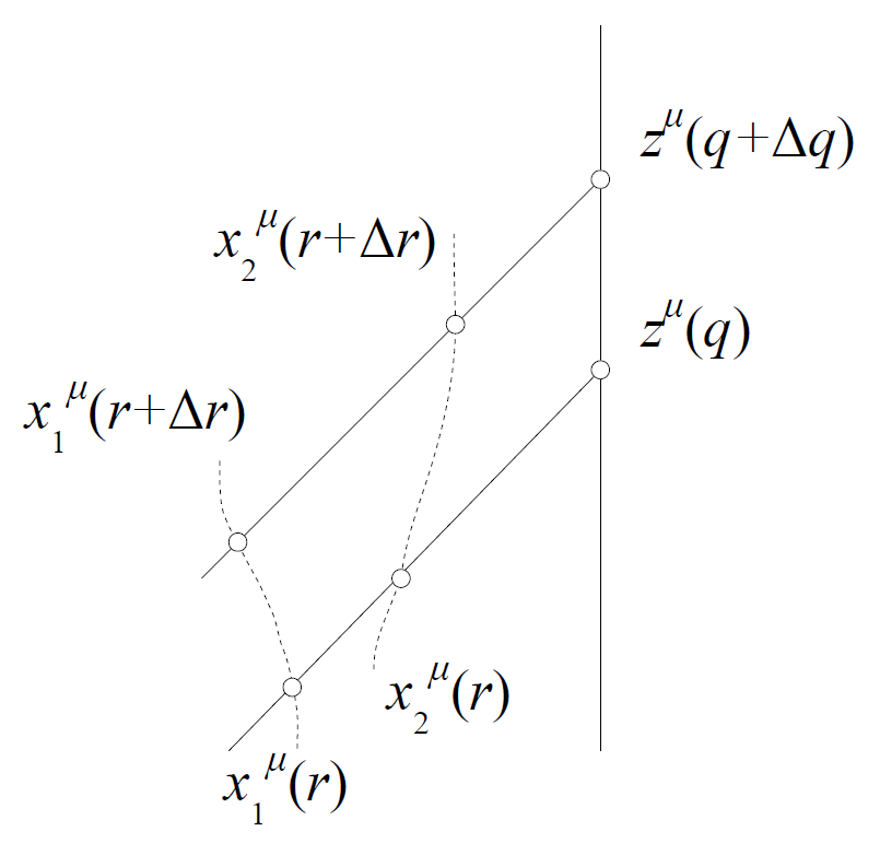
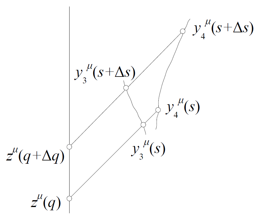
Figure 3: Splitting the source-detector relation into two steps (the stage between the two crossing points; the stage behind the second crossing point will look analogously, see Fig. 5). Left: Two types of relations between the world-lines of the source, $x_{j}^{\mu}(r)$, $j=1,2$, and those of the rest-frame detectors, $z^{\mu}(q)$ (the source either moves toward the detector or escapes from it). Right: Similar relations between the world-lines of the rest-frame source, $z^{\mu}(q)$, and those of the detectors, $y_{k}^{\mu}(s)$, $k=3,4$. Events $x_{j}^{\mu}$, $z^{\mu}$, and $y_{k}^{\mu}$ are causally related by null vectors.

Assume the three world-lines are restricted to some $t$-$z$ plane of the Minkowski space,

$$r \mapsto x^{\mu}(r)=\big{(}x^{0}(r),0,0,x^{3}(r)\big{)},$$ (9)

$$s \mapsto y^{\mu}(s)=\big{(}y^{0}(s),0,0,y^{3}(s)\big{)},$$ (10)

$$q \mapsto z^{\mu}(q)=\big{(}q,0,0,0\big{)}.$$ (11)

The metric has signature $(+,-,-,-)$ and we in general simplify notation by skipping the two vanishing components. The parametrizations are given in terms of proper times,

$$x^{\mu}(r+\Delta r) = x^{\mu}(r)+\Delta x^{\mu}(r),$$ (12)

$$y^{\mu}(s+\Delta s) = y^{\mu}(s)+\Delta y^{\mu}(s),$$ (13)

$$\dot{x}_{\mu}(r)\dot{x}^{\mu}(r) = \dot{y}_{\mu}(s)\dot{y}^{\mu}(s)=\dot{z}_{\mu}(q)\dot{z}^{\mu}(q)=1.$$ (14)

The dots represent proper-time derivatives. The world-vectors $y^{\mu}(s)-z^{\mu}(q)$, $z^{\mu}(q)-x^{\mu}(r)$, $y^{\mu}(s+\Delta s)-z^{\mu}(q+\Delta q)$, and $z^{\mu}(q+\Delta q)-x^{\mu}(r+\Delta r)$ are null.

We begin with establishing a relation between $\sigma^{2}=\Delta y_{\mu}(s)\Delta y^{\mu}(s)$, $\rho^{2}=\Delta x_{\mu}(r)\Delta x^{\mu}(r)$, and $\Delta q$. All the null vectors in Fig. 1 and Fig. 3 are parallel. In particular,

$$y^{\mu}(s+\Delta s)-z^{\mu}(q+\Delta q) = y^{\mu}(s)+\Delta y^{\mu}(s)-z^{\mu}(q)-\Delta z^{\mu}(q)\sim y^{\mu}(s)-z^{\mu}(q),$$ (15)

$$z^{\mu}(q+\Delta q)-x^{\mu}(r+\Delta r) = z^{\mu}(q)+\Delta z^{\mu}(q)-x^{\mu}(r)-\Delta x^{\mu}(r)\sim z^{\mu}(q)-x^{\mu}(r),$$ (16)

a fact implying that $\Delta y^{\mu}(s)-\Delta z^{\mu}(q)$ are $\Delta z^{\mu}(q)-\Delta x^{\mu}(r)$ are null as well. On the other hand, $\Delta x^{\mu}(r)$, $\Delta y^{\mu}(s)$, and $\Delta z^{\mu}(q)$ are timelike and future-pointing, so their relations can be parametrized by a hyperbolic coordinate,

$$\Delta z_{\mu}(q)\Delta y^{\mu}(s) = \sigma\Delta q\cosh\gamma,$$ (17)

$$\Delta z_{\mu}(q)\Delta x^{\mu}(r) = \rho\Delta q\cosh\chi.$$ (18)

Since $\Delta y^{\mu}(s)-\Delta z^{\mu}(q)$ and $\Delta z^{\mu}(q)-\Delta x^{\mu}(r)$ are null, we find

$$(\sigma/\Delta q)^{2}-2(\sigma/\Delta q)\cosh\gamma+1 = 0,$$ (19)

$$(\rho/\Delta q)^{2}-2(\rho/\Delta q)\cosh\chi+1 = 0.$$ (20)

Accordingly,

$$\sigma_{\pm}/\Delta q = \cosh\gamma\pm|\sinh\gamma|=e^{\pm|\gamma|},$$ (21)

$$\rho_{\pm}/\Delta q = \cosh\chi\pm|\sinh\chi|=e^{\pm|\chi|}.$$ (22)

Figure 4: The geometry between the two crossing points. Left: The geometry of the quadratic equation (19) and its two solutions $\sigma_{\pm}$ given by (21). The fact that $\sigma_{+}\geq\sigma_{-}$ implies $\sigma_{+}^{2}=\Delta y_{4\mu}(s)\Delta y_{4}^{\mu}(s)$, $\sigma_{-}^{2}=\Delta y_{3\mu}(s)\Delta y_{3}^{\mu}(s)$. Right: The geometry of the quadratic equation (20) and its two solutions $\rho_{\pm}$ given by (22). The fact that $\rho_{+}\geq\rho_{-}$ implies $\rho_{+}^{2}=\Delta x_{2\mu}(r)\Delta x_{2}^{\mu}(r)$, $\rho_{-}^{2}=\Delta x_{1\mu}(r)\Delta x_{1}^{\mu}(r)$.

Figure 5: Behind the second crossing point one finds $\sigma_{+}^{2}=\Delta y_{\mu}(s)\Delta y^{\mu}(s)$, $\rho_{-}^{2}=\Delta x_{\mu}(r)\Delta x^{\mu}(r)$, $\gamma(s)<0$, and $\chi(r)>0$.

In the limit $\Delta q\to 0$ we find two differential equations that link the three proper times,

$$\frac{ds(q)}{dq} = e^{\pm|\gamma(s(q))|},$$ (23)

$$\frac{dr(q)}{dq} = e^{\pm|\chi(r(q))|}.$$ (24)

Fig. 4 and Fig. 5 explain how to relate the signs in (23)–(24) with the signs of $\gamma(s(q))$ and $\chi(r(q))$. First of all, $\sigma_{+}\geq\sigma_{-}$ and $\rho_{+}\geq\rho_{-}$. For the stage between the crossing points this implies $\sigma_{+}^{2}=\Delta y_{4\mu}(s)\Delta y_{4}^{\mu}(s)$ and $\rho_{+}^{2}=\Delta x_{2\mu}(r)\Delta x_{2}^{\mu}(r)$. Secondly, the hyperbolic parameters are positive if the particle moves to the right, the case of the parts of the world-lines denoted in Fig. 4 by $\Delta y_{4}^{\mu}(s)$ and $\Delta x_{2}^{\mu}(r)$, and in Fig. 3 by $y_{4}^{\mu}(s)$ and $x_{2}^{\mu}(r)$. The same reasoning explains why the signs in $\sigma_{\pm}$ and $\rho_{\pm}$ are negative for $y_{3}^{\mu}(s)$ and $x_{1}^{\mu}(r)$, that is when the particles move to the left and thus the hyperbolic parameters are negative. Collecting all these cases we conclude that for trajectories whose shape is depicted in the left part of Fig. 1, the equations to solve are

$$\frac{ds(q)}{dq} = e^{\gamma(s(q))},$$ (25)

$$\frac{dr(q)}{dq} = e^{\chi(r(q))}.$$ (26)

The chain rule for derivatives thus implies

$$\frac{ds(q(r))}{dr} = e^{\gamma(s(q(r)))-\chi(r)}.$$ (27)

The situation changes behind the second crossing point (Fig. 5), where we find that $\gamma(s)$ is negative, $\gamma(s)=-|\gamma(s)|$ but the sign in $\sigma_{\pm}$ is positive. Hence,

$$\frac{ds(q)}{dq} = e^{|\gamma(s(q))|}=e^{-\gamma(s(q))}.$$ (28)

On the other hand, $\chi(r)$ is here positive, but the sign in $\rho_{\pm}$ is negative, hence

$$\frac{dr(q)}{dq} = e^{-|\chi(r(q))|}=e^{-\chi(r(q))}.$$ (29)

The chain rule for derivatives now implies

$$\frac{ds(q(r))}{dr} = e^{-\gamma(s(q(r)))+\chi(r)}.$$ (30)

In the next Section we restrict the analysis to the particular case of world-lines occurring for sources and detectors moving with constant accelerations.

III Uniformly accelerated sources and detectors

A particle that propagates along the world-line $t\mapsto(ct,0,0,z(t))$ with constant acceleration $a$, satisfies the Newton equation

$$\frac{d}{dt}\frac{v(t)}{\sqrt{1-\frac{v(t)^{2}}{c^{2}}}}=a,\quad v(t)=\frac{dz(t)}{dt}.$$ (31)

Its solution is given by

$$v(t) = c\frac{at+U}{\sqrt{c^{2}+(at+U)^{2}}},$$ (32)

$$z(t) = z(0)+\frac{c}{a}\sqrt{c^{2}+(at+U)^{2}}-\frac{c}{a}\sqrt{c^{2}+U^{2}}.$$ (33)

Here, $U$ is the initial world-velocity, $\bm{U}(0)=(0,0,U)$. The curve $t\mapsto\big{(}ct,z(t)\big{)}$ is a hyperbola parametrized by time $t$. The integrated proper time, $c^{2}d\tau^{2}=c^{2}dt^{2}-dz^{2}$, $\tau(0)=0$, when evaluated along the world-line, yields

$$c\tau(t) = (c^{2}/a)\arc\sinh(at/c+U/c)-(c^{2}/a)\arc\sinh(U/c).$$ (34)

Assuming $(ct(0),z(0))=(0,0)$, we find

$$\big{(}ct(\tau),z(\tau)\big{)} = \frac{c^{2}}{a}\Big{(}\sinh\big{(}a\tau/c+\arc\sinh(U/c)\big{)}-U/c,\cosh\big{(}a\tau/c+\arc\sinh(U/c)\big{)}-\sqrt{1+(U/c)^{2}}\Big{)}.$$ (35)

World-line (35) will play in our analysis the role of either $x^{\mu}(r)$ or $y^{\mu}(s)$ (we assume the source moves with positive constant acceleration, $a=\textrm{const}>0$, and initially negative world-velocity $U<0$; the detector acceleration is constant and negative, $b=\textrm{const}<0$, but its initial world-velocity is positive, $V>0$). To this end, let us write the two world-lines as follows (Fig. 6),

$$\big{(}x^{0}(r),x^{3}(r)\big{)} = \frac{1}{A}\big{(}\sinh(AR)-\sinh(-Ar+AR),\cosh(AR)-\cosh(-Ar+AR)\big{)},$$ (36)

$$\big{(}\dot{x}^{0}(r),\dot{x}^{3}(r)\big{)} = \big{(}\cosh(-Ar+AR),\sinh(-Ar+AR)\big{)}=\big{(}\cosh\chi(r),\sinh\chi(r)\big{)},$$ (37)

$$A = -a/c^{2}=-|A|,\quad a>0,$$ (38)

$$R = -(c^{2}/a)\arc\sinh(U/c)=|R|,\quad U<0,$$ (39)

$$\chi(r) = -Ar+AR=|A|r-|A|R,$$ (40)

$$\big{(}y^{0}(s),y^{3}(s)\big{)} = \frac{1}{B}\big{(}\sinh(BS)-\sinh(-Bs+BS),\cosh(BS)-\cosh(-Bs+BS)\big{)},$$ (41)

$$\big{(}\dot{y}^{0}(s),\dot{y}^{3}(s)\big{)} = \big{(}\cosh(-Bs+BS),\sinh(-Bs+BS)\big{)}=\big{(}\cosh\gamma(s),\sinh\gamma(s)\big{)},$$ (42)

$$B = -b/c^{2}=|B|,\quad b<0,$$ (43)

$$S = -(c^{2}/b)\arc\sinh(V/c)=|S|,\quad V>0,$$ (44)

$$\gamma(s) = -Bs+BS=-|B|s+|B|S.$$ (45)

Expressions such as $|A|R$ and $|B|S$ are independent of accelerations.

Figure 6: World-lines $x^{\mu}(r)$ (dashed) and $y^{\mu}(s(r))$ (full) given by (36)–(45), yet before the second crossing point, for $A=-1$, $R=0.5$, $B=1$, $S=1$, and $0\leq r\leq 1.4$ (in arbitrary units). The dotted line is on the light cone joining the endpoints of $x^{\mu}(r)$ and $y^{\mu}(s(r))$. This is the world-line of the light signal emitted at $x^{\mu}(r)$ and detected at $y^{\mu}(s(r))$.

III.1 Between the crossing points

The analysis given in the previous Section can be now directly applied to (36)–(45). Equations

$$\frac{ds(q)}{dq} = e^{\gamma(s(q))}=e^{-|B|s(q)+|B|S},\quad s(0)=0,$$ (46)

$$\frac{dr(q)}{dq} = e^{\chi(r(q))}=e^{|A|r(q)-|A|R},\quad r(0)=0,$$ (47)

imply

$$r(s) = \ln\left(1-\frac{|A|}{|B|}e^{-|A|R-|B|S}(e^{|B|s}-1)\right)^{-\frac{1}{|A|}},$$ (48)

$$s(r) = \ln\left(1+\frac{|B|}{|A|}e^{|A|R+|B|S}(1-e^{-|A|r})\right)^{\frac{1}{|B|}}.$$ (49)

The solution can be directly cross-checked by

$$\frac{ds(r)}{dr} = e^{\gamma(s(r))-\chi(r)},$$ (50)

with $\chi(r)$, $\gamma(s)$, and $s(r)$ given by (40), (45), and (49), respectively.

III.2 Behind the second crossing point

The second crossing point is determined by

$$\big{(}x^{0}(r),x^{3}(r)\big{)} = \big{(}y^{0}(s(r)),y^{3}(s(r))\big{)},\quad r>0,$$ (51)

where $s(r)$ is the solution (49). It occurs for $r=r_{1}$,

$$r_{1} = \frac{1}{|A|}\ln\frac{|A|e^{|A|R+|B|S}+|B|}{|A|e^{-|A|R-|B|S}+|B|},$$ (52)

$$s(r_{1}) = \frac{1}{|B|}\ln\frac{|A|+|B|e^{|A|R+|B|S}}{|A|+|B|e^{-|A|R-|B|S}}=s_{1},$$ (53)

and is located at

$$x^{0}(r_{1}) = y^{0}(s(r_{1}))$$ (54)

$$= 4\sinh(|A|R+|B|S)\frac{|A|\cosh{|B|S}+|B|\cosh{|A|R}}{(|A|e^{|A|R+|B|S}+|B|)(|A|e^{-|A|R-|B|S}+|B|)},$$ (55)

$$x^{1}(r_{1}) = y^{1}(s(r_{1}))$$ (56)

$$= 4\sinh(|A|R+|B|S)\frac{|A|\sinh{|B|S}-|B|\sinh{|A|R}}{(|A|e^{|A|R+|B|S}+|B|)(|A|e^{-|A|R-|B|S}+|B|)}.$$ (57)

Behind the second crossing point we have to solve

$$\frac{ds(q)}{dq} = e^{-\gamma(s(q))}=e^{|B|s(q)-|B|S},$$ (58)

$$\frac{dr(q)}{dq} = e^{-\chi(r(q))}=e^{-|A|r(q)+|A|R},$$ (59)

which is equivalent to

$$\frac{ds(r)}{dr} = e^{-\gamma(s(r))+\chi(r)}.$$ (60)

Collecting the above two cases, one finds that

$$s(r) = \left\{\begin{array}[]{rl}\frac{1}{|B|}\ln\left(1+\frac{|B|}{|A|}e^{|A|R+|B|S}(1-e^{-|A|r})\right),&0\leq r\leq r_{1},\\ -\frac{1}{|B|}\ln\left(1-\frac{|B|}{|A|}e^{-|A|R-|B|S}(e^{|A|r}-1)\right),&r_{1}\leq r<r_{\rm max},\end{array}\right.$$ (63)

is a solution to

$$\frac{ds(r)}{dr} = \left\{\begin{array}[]{rl}e^{\gamma(s(r))-\chi(r)},&0\leq r\leq r_{1},\\ e^{-\gamma(s(r))+\chi(r)},&r_{1}\leq r<r_{\rm max}.\end{array}\right.$$ (66)

In (63) the case $0\leq r\leq r_{1}$ corresponds to (49). $s(r)$ is continuous at $r_{1}$ but its derivative (66) is not. Let us note that $r$ is limited by its maximal value

$$r_{\rm max} = \frac{1}{|A|}\ln\left(1+\frac{|A|}{|B|}e^{|A|R+|B|S}\right)$$ (67)

with $s(r_{\rm max})=\infty$. At the event horizon, i.e. for $r\geq r_{\rm max}$, the source becomes invisible to the detector, but

$$\lim_{B\to 0}r_{\rm max}=\infty.$$ (68)

A detector at rest can monitor the accelerated system forever.

The inverse map, $r(s)$, reads

$$r(s) = \left\{\begin{array}[]{rl}-\frac{1}{|A|}\ln\left(1-\frac{|A|}{|B|}e^{-|A|R-|B|S}(e^{|B|s}-1)\right),&0\leq s\leq s_{1},\\ \frac{1}{|A|}\ln\left(1+\frac{|A|}{|B|}e^{|A|R+|B|S}(1-e^{-|B|s})\right),&s_{1}\leq s,\end{array}\right.$$ (71)

with $s_{1}=s(r_{1})$ given by (53). In particular, $r(\infty)=r_{\rm max}$, as expected.

Figure 7: Function $r(s)$ given by (71) for the same parameters as in Fig. 6. The point of second crossing, $s=s_{1}$, is visible as the point of non-differentiability of $r(s)$. The dotted line is the asymptotic value $r_{\rm max}=r(\infty)$ occurring at the event horizon.

IV Effective non-exponential decay

We are ready to write the final formula for the probability measured by the detector,

$$P(s) = e^{-r(s)/r_{0}}$$ (72)

$$= \left\{\begin{array}[]{rl}\left(1-\frac{|A|}{|B|}e^{-|A|R-|B|S}(e^{|B|s}-1)\right)^{\frac{1}{|A|r_{0}}},&0\leq s\leq s_{1},\\ \left(1+\frac{|A|}{|B|}e^{|A|R+|B|S}(1-e^{-|B|s})\right)^{-\frac{1}{|A|r_{0}}},&s\geq s_{1}\end{array}\right.$$ (75)

with

$$s_{1}=\frac{1}{|B|}\ln\frac{|A|+|B|e^{|A|R+|B|S}}{|A|+|B|e^{-|A|R-|B|S}},$$ (76)

and

$$P(\infty)=e^{-r_{\rm max}/r_{0}}.$$ (77)

Formulas (36)–(45) imply $|A|=|a|/c^{2}$, $|B|=|b|/c^{2}$,

$$e^{\pm|A||R|} = (U_{0}\pm|U|)/c,$$ (78)

$$e^{\pm|B||S|} = (V_{0}\pm|V|)/c,$$ (79)

where $(U_{0},0,0,U)$ and $(V_{0},0,0,V)$ are the initial world-velocities of the source and the detector, respectively. This ends the derivation of formula (4).

We can directly compare (75) with the probability postulated in [1],

$$P(s) = \left(1+\frac{\lambda}{\mu}\left(e^{(q-1)\mu s}-1\right)\right)^{-\frac{1}{q-1}},$$ (80)

in order to fit the protein folding data from [2, 3], and employed in [4] in fitting Zipf-law data from 36 plays by Shakespeare and 56 books by Dickens. Although there is no reason to believe that there are any links between the statistics of muon decays and frequencies of words used by Shakespeare, it is nevertheless intriguing that the same non-evident functional dependence on parameters is found.

In the limit $B\to 0$, corresponding to the detector moving with constant velocity, we obtain a power law,

$$\lim_{B\to 0}P(s) = \left\{\begin{array}[]{rl}\left(1-|A|e^{-|A|R}e^{-|B|S}s\right)^{\frac{1}{|A|r_{0}}},&0\leq s\leq s_{1},\\ \left(1+|A|e^{|A|R}e^{|B|S}s\right)^{-\frac{1}{|A|r_{0}}},&s\geq s_{1}\end{array}\right.$$ (83)

$$= \left\{\begin{array}[]{rl}\left(1-|a|(U_{0}-|U|)(V_{0}-|V|)s/c^{3}\right)^{\frac{c^{2}}{|a|r_{0}}},&0\leq s\leq s_{1},\\ \left(1+|a|(U_{0}+|U|)(V_{0}+|V|)s/c^{3}\right)^{-\frac{c^{2}}{|a|r_{0}}},&s\geq s_{1}.\end{array}\right.$$ (86)

with

$$s_{1}=2\frac{\sinh(|A|R+|B|S)}{|A|}=2\frac{U_{0}|V|+|U|V_{0}}{|a|}.$$ (87)

Fig. 2 shows $P(s)$ for $r_{0}=1$ and various values of the remaining parameters.

V Relativistic clocks and watches

Our result, as based on special relativity, cannot be in conflict with the standard tests of time dilation [12, 13]. The experiments were always designed to measure directly the decay, and not the decay products. Our conclusions may thus have some consequences for astrophysical or accelerator observations of atomic or particle lifetimes, but at this stage we cannot say anything more concrete.

Yet, it should be mentioned that Fig. 6 suggests another perspective on the subject of the paper. Namely, let us note that both $r$ and $s(r)$ are proper times measured by clocks propagating along the two world-lines. $s(r)$ is the proper time registered by the detector at the moment it detects (i.e. observes) the light signal emitted at proper time $r$ (as measured by the clock of the source). The clock of the source thus plays the role of a watch. An observer propagating along $s\mapsto y^{\mu}(s)$ sees at his proper time $s(r)$ the time $r$ as it appears on the clock of the source located at $x^{\mu}(r)$. The relation between the time $r$ of emission and the time $s(r)$ of observation is one-to-one. Therefore if we watch a decaying accelerating system, what we see is not the exponential decay but a generalized power law.

References

[1]Tsallis, C., Bemski, G. , and Mendes, R. S. Is re-association in folded proteins a case of nonextensivity?, Phys. Lett. A1999, 257, 93.
[2]Austin, R. H. et al., Activation energy spectrum of a biomolecule: Photodissociation of carbonmonoxy myoglobin at low temperatures, Phys. Rev. Lett.1974, 32, 403.
[3]Austin, R. H. et al., Dynamics of ligand binding to myoglobin, Biochemistry1975, 14, 5355.
[4]Montemurro, M. A. Beyond the Zipf–Mandelbrot law in quantitative linguistics, Physica A2001, 300, 567.
[5]Czachor, M. and Naudts, J. Thermostatistics based on Kolmogorov–Nagumo averages: Unifying framework for extensive and nonextensive generalizations, Phys. Lett. A2002, 298, 369.
[6]Rényi, A. Some fundamental questions of information theory, MTA III. Oszt. Közl.1960, 10, 251. Reprinted in Selected Papers of Alfréd Rényi, Turán, P. (Ed.); Akadémiai Kiadó, Budapest, 1976.
[7]Kolmogorov, A. N. Sur la notion de la moyenne, Atti. Acad. Naz. Lincei. Rend.1930, 12, 388. Reprinted in Selected Works of A. N. Kolmogorov. Vol.1. Mathematics and Mechanics, Tikhomirov, V. M. (Ed.); Kluwer, Dordrecht, 1991.
[8]Nagumo, M. Uber eine Klasse der Mittelwerte, Japan J. Math.1930, 7, 71. Reprinted in Mitio Nagumo Collected Papers, Yamaguti, M, Nirenberg, L., Mizohata, S., and Sibuya, Y. (Eds.); Springer, Tokyo, 1993.
[9]Jizba, P. and Arimitsu, T. The world according to Rényi: Thermodynamics of fractal systems,
AIP Conf. Proc.2001, 597, 341.
[10]Jizba, P. and Arimitsu, T. Observability of Rényi’s entropy, Phys. Rev. E2004, 69, 026128.
[11]Naudts, J. Generalised Thermostatistics, Springer, London, 2011.
[12]Rossi, B. and Hall, D. B. Variation of the rate of decay of mesotrons with momentum, Phys. Rev.1941, 59, 223.
[13]Frisch, D. and Smith, J. Measurement of the relativistic time dilation using mesons, Am. J. Phys.1963, 31, 342.