Covariance in Fractional Calculus

Abstract

Based on the requirement of covariance, we propose a new approach for generalizing fractional calculus in multi-dimensional space. As a first application we calculate an approximation for the ground state energy of the fractional 2-dimensional harmonic oscillator using the Ritz variational principle.

PACS numbers:

1 Introduction

The first applications of fractional calculus [Podlubny (1999), Hilfer (2000)] were developed in 1-dimensional Cartesian space, where problems were defined using a single coordinate:

As an example, Abel’s treatment of the tautochrone problem used the path-length $s$ [Abel (1823)].

In a similar way, as long as fractional calculus is understood as a framework for investigating memory effects such as investigating the influence of history on current developments, implementing causal and anti-causal properties or describing phenomena like anomalous diffusion processes [Metzler and Klafter (2000)] or causal elastic waves [Nasrolahpour (2013)] these processes are time-dependent and can be treated using a single time coordinate $t$.

While there is a long tradition in the theory of fractional calculus on $R^{n}$ [Samko (1993), Podlubny (1999)], practical interest in the multi-dimensional generalization of fractional calculus in Cartesian space, particularly for fractional wave equations, began with Raspini’s work on the fractional Dirac equation, which introduced derivatives of order $\alpha=2/3$ [Raspini (2000)], and has recently gained increasing interest [Tarasov (2021), Tarasov (2023), Kostić (2024)].

When extending fractional calculus to higher-dimensional spaces, ensuring covariance is essential. This requires that the definition of the fractional derivative and the corresponding fractional differential equations remain invariant under arbitrary coordinate transformations which is fundamental to the general validity of the results derived [Misner (1973), Lee (2018)].

2 Covariant transition from local to non-local operators

We define the requirement of covariance as form invariance under coordinate transformations, which on $R^{n}$ leave the line element $ds^{2}$ invariant [Adler (1975)]:

$$ds^{2}=g_{ij}dx^{i}dx^{j}\qquad i,j=1,...,n$$ (1)

and the components of the metric tensor $g_{\mu\nu}$ transform as a tensor of rank 2:

$$g_{kl}=\frac{\partial^{i}}{\partial^{k}}\frac{\partial^{j}}{\partial^{l}}g_{ij}\qquad\qquad i,j,k,l=1,...,n$$ (2)

In the following, we will present a covariant 2-step procedure to extend an arbitrary local operator to the fractional case by applying a convolution with a weakly singular kernel.

We compose a general covariant fractional operator $\tilde{\mathcal{O}}_{\textrm{type}}(w)$ as a combination of two covariant components, the classical local operator $\tilde{\mathcal{L}}$ and a non-localization operator $\tilde{\mathcal{G}}(w)$ with covariant kernel $w$:

• The classical local operator $\tilde{\mathcal{L}}$ is the basic constituent of almost all classical field theories of physics e.g. classical particle physics (Hamiltonian H), electro-dynamics (Maxwell equations), quantum mechanics (Schrödinger-, Klein-Gordon-, Dirac- equation), gauge theories (Yang-Mills theory) or cosmology (Einstein filed equations, string-theories) assumed to transform as a tensor of given rank.

• The non-localization operator $\tilde{\mathcal{G}}(w)$ is given as a convolution integral with a covariant kernel $w$.

Combining these two operators in a 2 step transition procedure from local to fractional operators may be realized as two different operator sequences:

A Riemann type sequence, where first the non-localization operator is applied followed by the classical operator:

$$\tilde{\mathcal{O}}_{\textrm{R}}(w)=\tilde{\mathcal{L}}\cdot\tilde{\mathcal{G}}(w)\ast$$ (3)

A Caputo type sequence with inverted operator succession, where first the classical operator is applied followed by the non-localization operator:

$$\tilde{\mathcal{O}}_{\textrm{C}}(w)=\tilde{\mathcal{G}}(w)\ast\tilde{\mathcal{L}}\cdot$$ (4)

Both types of a fractional operator will be used in the following.

The local operator $\tilde{\mathcal{L}}$ should transform as a tensor of a given rank $m$.

A classical example is the Laplace-operator contracted to a tensor of rank 0 (scalar) used in wave equations:

$$\bigtriangleup\Psi = \nabla^{j}\nabla_{j}\Psi$$ (5)

$$= g^{ij}\nabla_{i}\nabla_{j}\Psi\qquad\qquad i,j=1,...,N$$ (6)

$$= g^{ij}(\partial_{i}\partial_{j}-\left\{\begin{array}[]{c}k\\ ij\\ \end{array}\right\}\partial_{k})\Psi$$ (9)

$$= \frac{1}{\sqrt{g}}\partial_{i}\,g^{ij}\sqrt{g}\,\partial_{j}\Psi$$ (10)

where $\left\{\begin{array}[]{c}k\\ ij\\ \end{array}\right\}$ being the Christoffel symbol

$$\left\{\begin{array}[]{c}k\\ ij\\ \end{array}\right\}=\frac{1}{2}g^{kl}(\partial_{i}g_{jl}+\partial_{j}g_{il}-\partial_{l}g_{ij})$$ (11)

$g$ is the determinant of the metric tensor, $g=\det g_{ij}$ (2) and $\nabla$ is the covariant derivative [Adler (1975), Misner (1973)].

We postulate, that the fractional extension of a given local operator should not change the rank of the local operator. The fractional extension of a wave-equation should remain a wave-equation with corresponding tensor characteristics, the fractional extension of the Fokker-Planck-equation should exhibit the same tensor properties as the local one.

Therefore the non-localization operator $\tilde{\mathcal{G}}(w)$ may only transform as a tensor of rank 0 (scalar). This is realized as long as the weight is a function of the line element only.

$$w(h)\equiv w(\sqrt{ds^{2}})$$ (12)

An obvious choice is the weakly singular power law kernel used in Riesz potentials, which conserve the requirements of isotropy and homogeneity on $R^{n}$ [Tarasov (2018), Diethelm (2020)]:

$$w(h)=|h|^{-\alpha}\qquad\alpha>0$$ (13)

The covariant non-localization operator $\tilde{\mathcal{G}}(w)$ is realized as the integral on a second independently chosen coordinate space $h=\{h_{1},h_{2},...,h_{n}\}$

$$\tilde{\mathcal{G}}(w)=\frac{1}{N}\int_{R^{n}}dV\,w(h)\,$$ (14)

with the invariant volume element $dV=d^{n}h\,\sqrt{g}$ and a norm $N$.

We are free to choose two different coordinate systems for the local operator $\tilde{\mathcal{L}}$ and the convolution $\tilde{\mathcal{G}}$.

E.g. on $R^{2}$ the problem of calculating the spectrum of a rectangular membrane may be best formulated using in Cartesian coordinates $x=\{x,y\}$, but the corresponding convolution with Riesz kernel (13) may be best solved using polar coordinates $h=\{h_{r},h_{\phi}\}$.

We now have proposed the general strategy to obtain multi-dimensional covariant fractional extensions of classical tensor operators.

In the following we will give an example how to apply the presented method to obtain the fractional analogue of the classical Laplace operator.

We will derive the fractional kinetic energy operator of the classical 2-dimensional Schrödinger equation and will then give an upper limit for the ground state energy of the fractional Schrödinger equation with fractional harmonic oscillator potential using the Ritz variation principle [Ritz (1909), Gross (1988), Leissa (2005)] .

3 The Ritz variational principle and the ground state energy of the 2-dimensional fractional harmonic oscillator

The Ritz variational principle is widely used in quantum mechanics to optimize parametrized wave functions by minimizing the corresponding energy expectation value [Ritz (1909), Gross (1988), Leissa (2005)]

We will demonstrate the validity of the above proposed procedure by approximating the ground state energy $E_{0}$ for the 2-dimensional fractional Schrödinger equation.

We will first derive the fractional extension of the classical Schrödinger equation and then calculate the expectation value for a 2-dimensional Gaussian trial function.

The classical 2-dimensional Schrödinger equation in natural units ($m=c=\hbar=1$) is given in Cartesian coordinates $x=\{x,y\}$ as the sum of kinetic and potential energy operators:

$$H=T+V=\left(-{1\over 2}\Delta+V(x,y)\right)\Phi(x,y)=E\Phi(x,y)$$ (15)

with the harmonic oscillator potential ($r^{2}=x^{2}+y^{2}$)

$$V={1\over 2}(x^{2}+y^{2})={1\over 2}r^{\,2}$$ (16)

The fractional Schrödinger equation is the extended version of classical (15) and in natural units ($m=c=\hbar=D_{\alpha/2}=D_{\beta/2}=1$) given as the sum of the fractional extension of kinetic and potential energy [Herrmann (2018)] ( $D_{\alpha/2},D_{\beta/2}$ are dimensional factors to ensure correct kinetic and potential energy units in the fractional case):

$$H^{\alpha,\beta}=T^{\alpha/2}+V^{\beta/2}=\left(-{1\over 2}\Delta^{\alpha/2}+V^{\beta/2}(x,y)\right)\Phi(x,y)=E\Phi(x,y)\qquad 0\leq\alpha\leq 2$$ (17)

with the fractional harmonic oscillator potential ($r^{2}=x^{2}+y^{2}$)

$$V^{\beta/2}(x,y)={1\over 2}(x^{2}+y^{2})^{\beta/2}={1\over 2}r^{\,\beta}\qquad\qquad\qquad\qquad\qquad\qquad\beta,r\geq 0$$ (18)

Obviously (17) reduces to the classical Schrödinger equation (15) with the standard harmonic oscillator potential for the cases $\alpha=\beta=2$.

The Ritz method gives an upper limit $E$ for the ground state energy $E_{0}$ for the the fractional stationary Schrödinger equation and is given by the expectation values:

$$E_{0}\leq E={\braket{\Psi}{H^{\alpha,\beta}}{\Psi}\over\braket{\Psi}{\Psi}}={\braket{\Psi}{T^{\alpha/2}+V^{\beta/2}}{\Psi}\over\braket{\Psi}{\Psi}}$$ (19)

with a trial function $\Psi$ of the general form

$$\Psi=\sum_{i=0}^{n}c_{i}\psi_{i}$$ (20)

We will consider two coordinate systems, namely Cartesian and polar and the two possible operator sequences according to Riemann and Caputo.

First we define the covariant non-localization operators with proper normalization $N$ and will then calculate the expectation values for norm $\braket{\Psi}{\Psi}$, potential energy $\braket{\Psi}{V^{\beta/2}}{\Psi}$ and kinetic energy $\braket{\Psi}{T^{\alpha/2}}{\Psi}$ for a trial function $\ket{\Psi}$:

Using Cartesian coordinates on $R^{2}$ we obtain for the non-localization operator $\tilde{\mathcal{G}}$:

$$\tilde{\mathcal{G}}_{c}=\frac{1}{N}\int_{-\infty}^{\infty}dh_{x}\int_{-\infty}^{\infty}dh_{y}\,w(h_{x},h_{y})\qquad\qquad 0\leq\alpha\leq 2$$ (21)

Equivalently, introducing polar coordinates on $R^{2}$ and $dV=\sqrt{g}=h_{r}$:

$$\tilde{\mathcal{G}}_{p}=\frac{1}{N}\int_{0}^{\infty}dh_{r}\,h_{r}\int_{0}^{2\pi}dh_{\phi}\,w(h_{r},h_{\phi})\qquad\qquad 0\leq\alpha\leq 2$$ (22)

In both cases, we use a covariant kernel.

The norm $N$ is determined by the requirement that the eigenvalue spectrum or Fourier transform of $\tilde{\mathcal{G}}$ with the covariant Riesz kernel (13) should yield:

$$(\mathcal{F}\ast\tilde{\mathcal{G}})(k)=(\mathcal{F}\ast\tilde{\mathcal{G}}_{c})(k)=(\mathcal{F}\ast\tilde{\mathcal{G}}_{p})(k)=|k|^{\alpha-2}$$ (23)

which results in:

$$N=2^{2-\alpha}{\Gamma(1-\alpha/2)\over\Gamma(\alpha/2)}$$ (24)

We interpret the operator $\Delta^{\alpha/2}$ in (17) as a fractional extension of the classical Laplace operator (5).

With the covariant Riesz kernel (13), the fractional extension of the local Laplace operator is given using the Caputo-like sequence (4):

$$\Delta^{\alpha/2}_{C}={\Gamma(\alpha/2)\over 2^{2-\alpha}\Gamma(1-\alpha/2)}\int_{0}^{\infty}dh_{r}\,h_{r}^{1-\alpha}\int_{0}^{2\pi}dh_{\phi}\,\Delta$$ (25)

or, using the Riemann type sequence (3):

$$\Delta^{\alpha/2}_{R}={\Gamma(\alpha/2)\over 2^{2-\alpha}\Gamma(1-\alpha/2)}\,\Delta\int_{0}^{\infty}dh_{r}\,h_{r}^{1-\alpha}\int_{0}^{2\pi}dh_{\phi}$$ (26)

We will evaluate (19) with a rotationally invariant Gaussian trial function:

$$\ket{\Psi}=e^{-{1\over 2}\kappa^{2}(x^{2}+y^{2})}=e^{-{1\over 2}\kappa^{2}r^{2}}$$ (27)

where $1/\kappa$ is a measure for the width of the Gaussian.

For this trial function, we obtain for the norm

$$\braket{\Psi}{\Psi} = \pi\kappa^{-2}$$ (28)

and for the potential energy expectation value

$$\braket{\Psi}{V^{\beta/2}}{\Psi} = \braket{\Psi}{{1\over 2}(x^{2}+y^{2})^{\beta/2}}{\Psi}=\braket{\Psi}{{1\over 2}r^{\,\beta}}{\Psi}={1\over 2}\pi\kappa^{-\beta-2}\Gamma(1+\beta/2)$$ (29)

To evaluate the kinetic energy term in (19) we will discuss both, the Riemann type and the Caputo type fractional extension of the Laplace operator respectively.

Working with the Riemann type sequence (3) we first obtain for $\tilde{\mathcal{G}}\ket{\Psi}$ in Cartesian and polar coordinates respectively:

$$\tilde{\mathcal{G}}\ket{\Psi}=\tilde{\mathcal{G}}_{c}\ket{\Psi}=\tilde{\mathcal{G}}_{p}\ket{\Psi}=2^{\alpha/2-1}\kappa^{-2+\alpha}\Gamma(\alpha/2)L_{\alpha/2-1}({\kappa^{2}r^{2}\over 2})\ket{\Psi}$$ (30)

where $L_{q}(z)$ is the Laguerre polynomial of order $q$.

In a second step we apply the local Laplace operator $\Delta$, either in Cartesian $\Delta_{c}$ and polar coordinates $\Delta_{p}$ respectively, which results in:

$$\Delta^{\alpha/2}_{R}\ket{\Psi} = \Delta\tilde{\mathcal{G}}\ket{\Psi}$$ (31)

$$= \Delta_{c}\tilde{\mathcal{G}}_{p}\ket{\Psi}=\Delta_{c}\tilde{\mathcal{G}}_{c}\ket{\Psi}=\Delta_{p}\tilde{\mathcal{G}}_{p}\ket{\Psi}=\Delta_{p}\tilde{\mathcal{G}}_{c}\ket{\Psi}$$ (32)

$$= 2^{\alpha/2-1}\kappa^{\alpha}\Gamma(\alpha/2)\times$$

$$\left((k^{2}-2)L_{\alpha/2-1}({\kappa^{2}r^{2}\over 2})+(k^{2}-1)L^{1}_{\alpha/2-2}({\kappa^{2}r^{2}\over 2})\right.+$$

$$\,\,\,\,\left.(k^{2}-1)L^{1}_{\alpha/2-2}({\kappa^{2}r^{2}\over 2})+k^{2}r^{2}L^{2}_{\alpha/2-3}({\kappa^{2}r^{2}\over 2})\right)\ket{\Psi}$$

where $L_{q}^{p}(z)$ gives the generalized Laguerre polynomial order $q$.

With (3) we have applied our 2-step procedure to obtain the action of the fractional Laplace operator on the Gaussian trial function (27) according to the Riemann type sequence (3).

We may now use this result (3) to calculate the expectation value of the kinetic energy term in (19). We get the remarkably simple final result:

$$\braket{\Psi}{T^{\alpha}}{\Psi} = \braket{\Psi}{-{1\over 2}\Delta^{\alpha/2}_{R}}{\Psi}={1\over 2}\pi\kappa^{\alpha-2}\Gamma(1+\alpha/2)$$ (34)

The ground state energy follows with (34),(29),(28) as:

$$E={\braket{\Psi}{T^{\alpha/2}+V^{\beta/2}}{\Psi}\over\braket{\Psi}{\Psi}}={1\over 2}\kappa^{\alpha}\Gamma(1+\alpha/2)+{1\over 2}\kappa^{-\beta}\Gamma(1+\beta/2)$$ (35)

Minimizing the energy with respect to $\kappa$ by solving the equation

$$\frac{\partial}{\partial\kappa}E(\kappa)=0$$ (36)

yields the optimum $\kappa_{opt}$:

$$\kappa_{opt}(\alpha,\beta)=\left({\beta\over\alpha}{\Gamma(1+\beta/2)\over\Gamma(1+\alpha/2)}\right)^{1/(\alpha+\beta)}$$ (37)

and the optimum energy $E_{opt}(\kappa_{opt})$:

$$E_{opt}(\alpha,\beta)={\alpha+\beta\over 2\alpha\beta}\bigl{(}\alpha\,\Gamma(1+\alpha/2)\bigr{)}^{\beta/(\alpha+\beta)}\bigl{(}\beta\,\Gamma(1+\beta/2)\bigr{)}^{\alpha/(\alpha+\beta)}$$ (38)

with the property $E_{opt}(\alpha,\beta)=E_{opt}(\beta,\alpha)$ as a direct consequence of the particle wave dualism which holds for the fractional extension of quantum mechanics too.

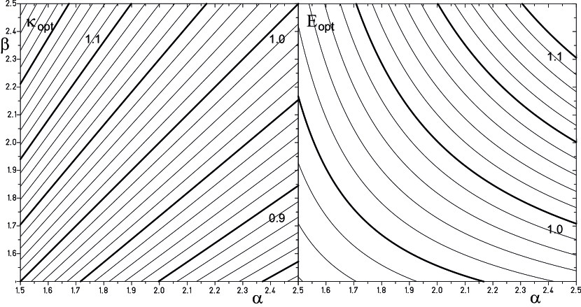
Figure 1: Left: The optimum $\kappa_{opt}$ from (37) Right:The optimum $E_{opt}$ from (38)

In Figure 1 we show the corresponding graphs of the optimum $\kappa_{opt}$ and $E_{opt}$.

Let us now compare these results with the Caputo type sequence (4) for a fractional extension of local operators for Cartesian and polar coordinates respectively for the local $\Delta=\{\Delta_{c},\Delta_{p}\}$ as well as the non-localization operator $\tilde{\mathcal{G}}=\{\tilde{\mathcal{G}}_{c},\tilde{\mathcal{G}}_{p}\}$.

With the same Gaussian trial function $\ket{\Psi}$ we evaluate:

$$\Delta^{\alpha/2}_{C}\ket{\Psi} = \tilde{\mathcal{G}}\ast\Delta\ket{\Psi}$$ (39)

$$= \tilde{\mathcal{G}}_{p}\ast\Delta_{c}\ket{\Psi}=\tilde{\mathcal{G}}_{c}\ast\Delta_{c}\ket{\Psi}=\tilde{\mathcal{G}}_{p}\ast\Delta_{p}\ket{\Psi}=\tilde{\mathcal{G}}_{c}\ast\Delta_{p}\ket{\Psi}$$ (40)

$$= \tilde{\mathcal{G}}\ast\kappa^{2}(\kappa^{2}r^{2}-2)\ket{\Psi}$$ (41)

$$= 2^{\alpha/2-1}\kappa^{\alpha}\Gamma(\alpha/2)\times$$

$$\left((\kappa^{2}-2)L_{\alpha/2-1}({\kappa^{2}r^{2}\over 2})+(\kappa^{2}-1)L^{1}_{\alpha/2-2}({\kappa^{2}r^{2}\over 2})\right.+$$

$$\,\,\,\,\left.(\kappa^{2}-1)L^{1}_{\alpha/2-2}({\kappa^{2}r^{2}\over 2})+\kappa^{2}r^{2}L^{2}_{\alpha/2-3}({\kappa^{2}r^{2}\over 2})\right)\ket{\Psi}$$

which is identical with (3) and consequently we obtain the same results for $\kappa_{opt}$ and $E_{opt}$ as before for the Riemann type fractional extension sequence for the Gaussian trial function.

We have demonstrated, that either choice of the coordinate system (Cartesian, polar) as well as either choice of the operator sequence (classical operator, non-localization convolution with the Riesz type kernel) calculating the fractional extension of the 2-dimensional Laplace operator leads to identical results.

This is a strong indication, that the proposed fractional generalization method yields reliable, valid results, which are independent of a specifically chosen coordinate set.

In addition, multi-dimensional fractional calculus provides new insights into mathematical and physical phenomena that were not evident in the 1-dimensional case. In the next section, we present some examples.

4 Multi-dimensionality, non-locality and new viewpoints

We have demonstrated that a covariant fractional extension of a standard local tensor operator can be successfully achieved through a 2-step process.

Additional intriguing aspects arise when extending fractional calculus from one-dimensional to multi-dimensional spaces.

In 1-dimensional fractional calculus, there are only a few distinct definitions of a fractional integral with a given singular kernel (see 13), which differ by setting different integral bounds.

In higher-dimensional spaces, the variety of possible region and topologies increases, as the number of degrees of freedom grows:

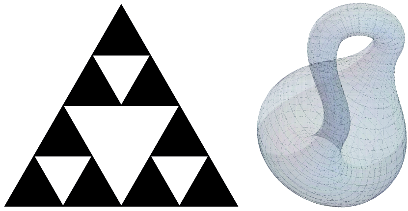
Figure 2: New regions in multi-dimensional fractional calculus include the correct treatment of new possible region types for the non-localization integral $\tilde{\mathcal{G}}$: On the left: the Sierpiński triangle (with recursion step = 3) a potential fractal region for the 2-dimensional non-localization operator and a typical example for self-similarity. On the right: the Klein bottle, an example of a volume with a non-orientable surface (modified version of [Senapon (2024)]).

Figure 2 illustrates new fascinating regions in multi-dimensional fractional calculus. On the left, we depict a Sierpiński triangle [Sierpiński (1916)] for a specific iteration step, representing one possible realization of a non-connected set of sub-regions for defining a fractional integral, and exhibiting typical fractal properties.

A notable challenge is integrating over a region like the Klein bottle (shown on the right of Figure 2), which exemplifies a volume with a non-orientable surface [Klein (1881)].

Another aspect of selecting an integration region arises with the covariant extension of the Caputo and Riemann fractional integrals, both of which are typically defined over only a portion of $R^{n}$ [Podlubny (1999), Herrmann (2018)]. Until now, the coordinate sets for the local operator and the non-local operator could be chosen independently. In the case of the Caputo and Riemann fractional integrals, these coordinate systems are already linked in the 1-dimensional case.

Another important aspect is the use of finite-range kernels. For example, in three-dimensional spherical coordinates, setting the integral bounds to $0\leq h_{r}\leq r$ instead of $0\leq h_{r}\leq\infty$ defines a spherical boundary, resulting in a finite-range potential with a sharp cut-off.

This can be viewed as an extreme case of tempered fractional calculus. In the context of nuclear physics, such a cut-off simulates a finite-range potential, akin to a generalized Yukawa-type potential, which describes the propagation of massive particles.

In one dimensional fractional calculus, a classical requirement for valid fractional convolution integrals is the restriction to weakly singular kernels [Diethelm (2020)]. In higher-dimensional spaces, however, this requirement should be interpreted more broadly.

To clarify this point:

Consider the 2-dimensional non-localization integral e.g. in Cartesian coordinates $\{p,m\}$

$$\tilde{\mathcal{G}}_{c}=\frac{1}{N}I_{2}(m)I_{1}(m,p)=\frac{1}{N}\int_{-\infty}^{\infty}dm\int_{-\infty}^{\infty}dp\,w(m,p)\qquad\qquad 0\leq\alpha\leq 2$$ (43)

This expression is a sequence of two 1-dimensional integrals, where the inner integral is given by:

$$I_{1}(m,p)=\int_{-\infty}^{\infty}dp\,w(m,p)=\int_{-\infty}^{\infty}dp\frac{1}{(p^{2}+m^{2})^{\alpha/2}}\qquad\qquad 0\leq\alpha\leq 2$$ (44)

with the covariant Riesz weight (13):

$$w(p,m)=\frac{1}{(p^{2}+m^{2})^{\alpha/2}}\qquad\qquad\qquad\qquad\qquad\qquad\qquad m^{2}\geq 0$$ (45)

which is singular only for the case $m=0$ and reduces to a non-singular but still non-local kernel for all $m^{2}>0$.

We may conclude that, in higher-dimensional fractional calculus, a non-singular kernel for all $ds>0$ is a direct consequence of the covariance requirement.

Extending the coordinate set to 4-dimensional Minkowski space-time $\{p_{x},p_{y},p_{z},t,m\}$ (45) may be interpreted as a key component in the formulation a generalized Feynman propagator for massive particles.

5 Conclusions

We have proposed a covariant transition from local to fractional operators, which is based on the requirement of covariance for the constituents involved: the local operator, the kernel and the non-localization (convolution) integral on $R^{n}$ leading to the fractional extended operator.

We have applied the proposed procedure to calculate an approximation of the ground state energy of the fractional harmonic oscillator and obtained an analytic formula using the Ritz variation principle.

The proposed non-localization procedure on an appropriately chosen metric establishes a connection between fractional calculus and generalized field theories. This will open new and promising insights and applications in e.g. cosmology or particle physics.

6 Acknowledgement

We thank A. Friedrich for useful discussions.

References

- [Abel (1823)] Abel, N. H. Solution de quelques problemes a l’aide d’integrales definies, oevres completes. Vol. 1 Grondahl, Christiana, Norway, 1823, 10,16–18
- [Adler (1975)] Adler, R., Bazin, M. and Schiffer, M., Introduction to general relativity. McGraw-Hill, New York (1975)
- [Diethelm (2020)] Diethelm, K., Garrappa, R., Giusti, A. and Stynes, M., Why fractional derivatives with nonsingular kernels should not be used. Fract. Calc. Appl. Anal., 2020, 23, 610–634,
- [Gross (1988)] Gross, E. K. U., Oliveira, L. N. and Kohn, W., Ritz variational principle for ensembles of fractionally occupied states Phys. Rev. A, 1988, 37, 2805–2808,
- [Herrmann (2018)] Herrmann, R., Fractional calculus - an introduction for physicists. 3rd ed., (2018) World Scientific Publ., Singapore
- [Hilfer (2000)] Hilfer, R., Applications of fractional calculus in physics. World Scientific Publ., Singapore (2000)
- [Klein (1881)] Klein, F. , Über Körper, welche von confocalen Flächen zweiten Grades begränzt sind. Math. Ann., 1881, 18, 410–427,
- [Kostić (2024)] Kostić, M., Multidimensional Fractional Calculus: Theory and Applications. Axioms 2024 13(9) 623,
- [Lee (2018)] Lee, J. M. , Introduction to Riemannian Manifolds. Springer, Berlin, Germany., (2018),
- [Leissa (2005)] Leissa, A. W., The historical bases of the Rayleigh and Ritz methods J. Sound and Vib. 2005 287, 961–978,
- [Metzler and Klafter (2000)] Metzler, R. and Klafter, J., The random walk’s guide to anomalous diffusion: a fractional dynamics approach. Phys. Rep. 2000 339, 1–77,
- [Misner (1973)] Misner, C. W., Thorne, K. S. and Wheeler, J. A. Gravitation. Freeman, San Francisco (1973)
- [Nasrolahpour (2013)] Nasrolahpour, H., A note on fractional electrodynamics. Commun. Nonlin. Sci. Numer. Simul. 2013, 25, 5–15,
- [Podlubny (1999)] Podlubny, I., Fractional differential equations. Academic Press, New York (1999)
- [Raspini (2000)] Raspini, A., Dirac equation with fractional derivatives of order 2/3. Fizika B, 2000, 9, 49–55,
- [Ritz (1909)] Ritz, W. , Über eine neue Methode zur Lösung gewisser Variationsprobleme der mathematischen Physik. J. für Reine u. Angew. Math., 1909, 195, 1–61
- [Samko (1993)] Samko, S. G., Kilbas, A. A. and Marichev, O. I., Fractional integrals and derivatives, Translated from the 1987 Russian original, Gordon and Breach, Yverdon (1993)
- [Sierpiński (1916)] Sierpiński, W. Sur une courbe cantorienne qui contient une image biunivoque et continue de toute courbe donnee. C. r. hebd. Seanc. Acad. Sci., 1916, 162, 629–632.
- [Senapon (2024)] Senapon, W. A., The Klein bottle, from Wolfram Demonstration Project, 2024, https://demonstrations.wolfram.com/TheKleinBottle/
- [Tarasov (2018)] Tarasov, V. E. No nonlocality. No fractional derivative. Commun. Nonlinear Sci. Numer. Simul., 2018, 62, 157–163,
- [Tarasov (2021)] Tarasov, V. E. , General fractional vector calculus. Mathematics, 2021 9, 2816
- [Tarasov (2023)] Tarasov, V. E. , General fractional calculus in multi-dimensional space: Riesz form Mathematics, 2023 11(7), 1651