Topological chiral superconductivity beyond paring in Fermi-liquid

Abstract

We investigate a mechanism to produce superconductivity by strong purely repulsive interactions, without using paring instability in Fermi-liquid. The resulting superconductors break both time-reversal and reflection symmetries in the orbital motion of electrons, and exhibit non-trivial topological order. Our findings suggest that this topological chiral superconductivity is more likely to emerge near or between fully spin-valley polarized metallic phase and Wigner crystal phase. Unlike conventional BCS superconductors in fully spin-valley polarized metals, these topological chiral superconductors are only partially spin-valley polarized, even though the neighboring normal state remains fully spin-valley polarized. The ratios of electron densities associated with different spin-valley quantum numbers are quantized as simple rational numbers. Furthermore, many of these topological chiral superconductors exhibit charge-4 or higher condensation. One of the topological chiral superconductors is in the same phase as the “spin”-triplet $p+\textrm{i}p$ BCS superconductor, while others are in different phases than any BCS superconductors. The same mechanism is also used to produce anyon superconductivity between fractional anomalous quantum Hall states in the presence of a periodic potential.

I Introduction

After the discovery of superconductivity in 1911 [1], the standard BCS mechanism for superconductivity was developed in 1957 [2], based on the electron pairing instability of Fermi liquid, caused by an effective attraction between electrons. In this paper, we explore a very different mechanism of superconductivity, which is caused by strong purely repulsive interaction. The superconductivity from our mechanism is very different from BCS superconductivity.

In fact, the mechanism based on the charged anyons in chiral spin liquid [3, 4, 5], and related models [6, 7, 8, 9, 10, 11, 12], belongs to this class of mechanism (i.e. driven by purely repulsive interactions). In this paper, we obtain superconductivity directly from electrons with repulsive interaction, without going through charged anyons and the associated anyon superconductivity. The resulting superconductivity may not be associated with electron pairing; charge-$4$ (and higher) condensation is also possible [11]. As a result, the resulting superconductivity usually carries non-trivial topological order [13, 14], which will be referred to as topological chiral superconductivity.

The idea behind this non-BCS mechanism is the following. We first assume that electron hopping amplitude is complex, due to spontaneous time reversal symmetry breaking and/or spin-orbit coupling. We also assume that electron interaction is larger than electron hopping energy. In this case, when electrons have an incommensurate density, they may not form a Fermi liquid.

Certainly, when interaction is weak, electrons will form a Fermi liquid. However, when interaction is strong, the electron motions are highly correlated. Since electron hopping is complex, the two electrons exchange their place via correlated motion, and the phase factor can be arbitrary. In this case, electrons may forget their Fermi statistics. Thus, electrons may form a superconducting state via the mechanism of anyon or boson superconductivity. The above idea is very rough, but may point to a right direction [12].

In this paper, we discuss a concrete realization of the above idea in 2-dimensional space. We argue that a strong repulsive interaction may cause a chiral superconductivity that spontaneously breaks time reversal and space reflection symmetry in orbital motion of electrons. Other sources of time-reversal symmetry breaking and/or spin-orbital coupling in orbital motion may further help this chiral superconductivity.

We will use the theory of anyon superconductivity developed in Ref. 8, 12. Since a fermion is a special case of anyon, the theory of anyon superconductivity applies to fermion superconductivity without change. We apply our theory to multi-layer graphene. We find many topological chiral superconductors driven by purely repulsive interaction, whose ground-state energies may be lower than those of fully spin-valley polarized Fermi liquid (referred to as quarter Fermi liquid) and Wigner crystal at low densities.

Quarter Fermi liquids and Wigner crystals have both been observed in experiments at low densities where the interaction effect is strong[15]. Furthermore, a strong coupling superconducting state that breaks time reversal and reflection symmetries in electron orbital motion was observed in Ref. 15 between quarter Fermi liquid and Wigner crystal, in tetralayer rhombohedral-stacked graphene without Moire pattern. Other superconductivities were also observed in bilayer [16, 17, 18, 19], trilayer [20, 21], and Moire-tetralayer [22] rhombohedral-stacked graphene systems. Some BCS-pairing mechanisms for those superconducting states were explored in Ref. 23, 24, 25, 26, 27, 28, 29, 30, 31.

If a superconducting state is observed close to a quarter Fermi liquid, as in Ref. 15, one might expect the superconducting state to be also fully spin-valley polarized. In this case, we need an effective attraction between electrons to induce the pairing instability of the Fermi liquid.

In this paper, we take a very different approach of using only strong repulsive interaction, which leads to very different chiral superconductors. The resulting chiral superconductors are not fully spin-valley polarized and are not induced by paring instability of Fermi liquid. Some of them are half spin-valley polarized (with two spin-valley components present and at equal density) while others are spin-valley un-polarized (with all four spin-valley components at equal density). We stress that, in our chiral superconductors, the ratio of different species of electrons are quantized as simple rational numbers. Thus, in contrast to BCS superconductors of quarter Fermi liquid, the transition from spin-valley partially-polarized chiral superconductors to quarter Fermi liquid cannot be continuous at zero temperature in the clean limit.

Also, as we lower the electron density, a topological chiral superconductor is likely to change into a Wigner crystal, also via a first order transition. Thus topological chiral superconductivity is more likely to appear near the transition between quarter Fermi liquid and Wigner crystal, since all those phases are driven by strong repulsive interactions. As a strong coupling superconductor, the coherence length of a chiral superconductor is about the same as the inter-electron separation.

All these chiral superconductors are topological (i.e. carry non-trivial topological order, where another example was given in Ref. 32); many of them have charge-4 or higher condensation and will break time reversal and space reflection symmetry in addition to carrying gapless chiral edge modes.

Our calculation is not reliable enough to predict if a chiral superconductor can appear or not (i.e. can have energy below both quarter Fermi liquid and Wigner crystal). However, if a chiral superconductor (i.e. a superconductor that breaks time reversal and reflection symmetry) is observed in experiments near quarter Fermi liquid and Wigner crystal as in Ref. 15, our calculation suggests that it may be a partially spin-valley polarized topological superconductor, with properties described above.

The calculated ground-state energies of these partially spin-valley polarized superconductors are lower, but still close to Hartree-Fock energy of a quarter Fermi liquid. To achieve a lower energy state than the quarter Fermi liquid, additional time-reversal symmetry breaking and/or spin-orbit interaction may be helpful. The strong geometric phase curvature near the bottom of the graphene band also contributes to breaking time-reversal symmetry through partial spin-valley polarization.

We remark that, although most topological chiral superconductors belong to different phases than BCS superconductors, one of the topological chiral superconductors (which we denote as the $K_{2a}$-chiral superconductor) belong to the same phase as the “spin”-triplet $p+\hskip 1.0pt\mathrm{i}\hskip 1.0ptp$ BCS superconductor. Here “spin” corresponds to a pair of spin-valley quantum numbers, and may not be the electron spin. Such a $K_{2a}$-chiral superconductor can be induced by a purely repulsive interaction. It can also be induced by a pairing instability of a half Fermi liquid caused by an effective attractive interaction. Here, half Fermi liquid refers to a Fermi liquid formed by two species of electrons of equal density. We note that very recently, a superconducting state has been observed next to a half Fermi liquid in rhombohedral trilayer graphene in Ref. 21. The $K_{2a}$-chiral superconductor also has similarly low energy to other chiral superconductors at lower densities. Thus, it may also appear near the quarter Fermi liquid and Wigner crystal, as in rhombohedral tetralayer graphene in Ref. 15.

In the second part of paper, we will use the same method to discuss possible anyon superconductivity between two fractional quantum anomalous Hall (FQAH) states. The periodic potential in FQAH states play a crucial role for the appearance of anyon superconductivity.

II Chiral superconductivity driven by purely repulsive interactions

To construct a topological chiral superconducting state, let us consider a simple case of spin-$\frac{1}{2}$ electrons in 2-dimension space. We view each electron as a bound state of a boson and $2\pi$-flux [33]. We then smear the $2\pi$-flux into a uniform “magnetic” field $\widetilde{b}$. In this case, the interacting spin-$\frac{1}{2}$ electrons are effectively described by interacting spin-$\frac{1}{2}$ bosons in a uniform magnetic field, with a filling fraction $\nu=1$. The interacting bosons can form various states that correspond to various states of interacting electrons.

When repulsive interaction is strong, the interacting bosons may form an incompressible fractional quantum Hall (FQH) state. In this case, the only low energy fluctuations are the co-fluctuations of the boson density and “magnetic” field $\widetilde{b}$ keeping the filling fraction $\nu=1$ fixed. Such co-fluctuations are gapless and are the only gapless modes of the system. In this case, the system is in a superconducting state (i.e. a superfluid state) [34].

We remark that this FQH state does not emerge from single-particle Landau levels produced by an external magnetic field; it has purely many-body origins. Under broken time-reversal symmetry, attaching $2\pi$ flux to the fields is an allowed operation which may lower the energy of the state. We model this with FQH wavefunctions, which are the simplest way to implement flux attachment while keeping density uniform. Indeed, the single-particle orbitals are not eigenstates of a kinetic energy operator without an external magnetic field, but they enforce 1. statistics consistent with flux attachment, 2. zeros in the wavefunction that favor repulsive interactions, and 3. uniform density apart from the superfluid mode controlled by a length scale $l_{b}$. The precise form of the many-body wavefunction may differ from the Laughlin states studied here, but we use these as representatives for phases which may arise from strong correlations.

For interacting spin-$\frac{1}{2}$ bosons with filling fraction $\nu=1$, the most natural FQH state is given by the following wave function

$$\Phi(z_{i}^{\uparrow},z_{i}^{\downarrow})=\hskip 1.0pt\mathrm{e}^{-\frac{\sum_{i}|z_{i}^{\uparrow}|^{2}+|z_{i}^{\downarrow}|^{2}}{4l_{b}^{2}}}\prod_{i<j}(z_{i}^{\uparrow}-z_{j}^{\uparrow})^{2}(z_{i}^{\downarrow}-z_{j}^{\downarrow})^{2}$$ (1)

where $z_{i}^{\uparrow},z_{i}^{\downarrow}$ are complex numbers describing the boson coordinates, and $l_{b}$ is the length scale of electron separation. Such a bosonic FQH state corresponds to the following electron wave function

$$\Psi(z_{i}^{\uparrow},z_{i}^{\downarrow}) =\hskip 1.0pt\mathrm{e}^{-\frac{\sum_{i}|z_{i}^{\uparrow}|^{2}+|z_{i}^{\downarrow}|^{2}}{4l_{b}^{2}}}\prod_{i<j}(z_{i}^{\uparrow}-z_{j}^{\uparrow})^{2}(z_{i}^{\downarrow}-z_{j}^{\downarrow})^{2}$$

$$\prod_{i<j}(z_{i}^{\uparrow*}-z_{j}^{\uparrow*})(z_{i}^{\downarrow*}-z_{j}^{\downarrow*})\prod_{i,j}(z_{i}^{\uparrow*}-z_{j}^{\downarrow*}),$$ (2)

where the factor $\prod_{i<j}(z_{i}^{\uparrow*}-z_{j}^{\uparrow*})(z_{i}^{\downarrow*}-z_{j}^{\downarrow*})\prod_{i,j}(z_{i}^{\uparrow*}-z_{j}^{\downarrow*})$ is the wave-function representation of the flux smearing operation.

The superconducting mode in this system is a co-fluctuation of up and down spins. Increasing the density of up spins in a region increases the effective magnetic field seen by the down spins, causing their density to increase to keep the filling fraction fixed. The increased down spin density in turn increases the effective magnetic field seen by the up spins, preserving their original filling fraction. These density fluctuations appear as fluctuations of $l_{b}$ in the wavefunction.

We now examine the energetics of this state. Let $N_{\uparrow}$ ($N_{\downarrow}$) be the total number of spin-$\uparrow$ (spin-$\downarrow$) electrons. The total angular momentum of the above state is

$$L_{z}^{\text{tot}} =N_{\uparrow}(N_{\uparrow}-1)+N_{\downarrow}(N_{\downarrow}-1)$$

$$\ \ \ \ -\frac{1}{2}N_{\uparrow}(N_{\uparrow}-1)-\frac{1}{2}N_{\downarrow}(N_{\downarrow}-1)-N_{\uparrow}N_{\downarrow}$$

$$=\frac{1}{2}(N_{\uparrow}-N_{\downarrow})^{2}-\frac{N_{\uparrow}+N_{\downarrow}}{2}.$$ (3)

We see that each pair of spin-$\frac{1}{2}$ electrons has an angular momentum $L_{z}=-1$, just like a spin triplet $p$-wave paired superconducting state. It is crucial that the leading $N$-contribution to the angular momentum of each electron is cancelled completely. Otherwise, the kinetic energy of the wave-function $\Psi(z_{i}^{\uparrow},z_{i}^{\downarrow})$ will be too high.

This cancellation can be seen by comparing the total angular momenta for $N_{\uparrow}=N_{\downarrow}$ system and $N_{\uparrow}=N_{\downarrow}+1$ system. We can also fix the position of all other electrons and consider the motion of, say, first spin-$\uparrow$ electron. From the wave function, we see that other spin-$\uparrow$ electrons behave like $2\pi$-flux quanta and other spin-$\downarrow$ electrons behave like $-2\pi$-flux quanta. The first spin-$\uparrow$ electron sees a zero average “magnetic” field. Thus its angular momentum does not contain a linear-$N$ term.

The electron wave-function $\Psi(z_{i}^{\uparrow},z_{i}^{\downarrow})$ has a third order zero between two spin-$\uparrow$ (spin-$\downarrow$) electrons, and has a first order zero between a spin-$\uparrow$ and a spin-$\downarrow$ electrons. So $\Psi(z_{i}^{\uparrow},z_{i}^{\downarrow})$ has a reduced interaction energy compared to Fermi liquid state. To estimate this reduction very roughly, we assume the interaction energy per electron to be

$$E_{\text{int}}=U\left\langle\frac{1}{n+1}\right\rangle$$ (4)

where $U$ is the interaction strength at distance $l_{b}$ and $\langle\frac{1}{n+1}\rangle$ is the average of inverse order of zeros (shifted by 1). For example, the wave-function $\Psi(z_{i}^{\uparrow},z_{i}^{\downarrow})$ has an interaction energy per electron

$$E_{\text{int}}=U\frac{\frac{1}{3+1}+\frac{1}{1+1}}{2}=\frac{3}{8}U.$$ (5)

In comparison, a Fermi liquid of spin-$\frac{1}{2}$ electrons has an interaction energy per electron

$$E_{\text{int}}=U\frac{\frac{1}{1+1}+\frac{1}{0+1}}{2}=\frac{3}{4}U,$$ (6)

since the order of zeros between two spin-$\uparrow$ (spin-$\downarrow$) electrons is 1 and the order of zeros between a spin-$\uparrow$ and a spin-$\downarrow$ electrons is 0, for the Fermi liquid.

The electron wave-function $\Psi(z_{i}^{\uparrow},z_{i}^{\downarrow})$ has a higher kinetic energy compared to the Fermi liquid, since each electron has a larger momentum. The typical momentum of each electron can be estimated as

$$p=(\langle n\rangle n_{e})^{1/2},$$ (7)

where $\langle n\rangle$ is the average of order of zeros and $n_{e}$ is the electron density. For $\Psi(z_{i}^{\uparrow},z_{i}^{\downarrow})$, we have

$$p=(n_{e}(3+1)/2)^{1/2}=\sqrt{2}n_{e}^{1/2},$$ (8)

while for Fermi liquid, we have

$$p=n_{e}^{1/2}((1+0)/2)^{1/2}=\frac{1}{\sqrt{2}}n_{e}^{1/2},$$ (9)

If the electron has an effective mass $m$, the chiral superconducting state will have an energy (per electron)

$$E_{\text{FQH}}=\frac{n_{e}}{m}+\frac{3}{8}U,$$ (10)

while the Fermi liquid will have an energy (per electron)

$$E_{\text{Fermi}}=\frac{n_{e}}{4m}+\frac{3}{4}U.$$ (11)

This will give us some idea when the chiral superconducting state is favored. Certainly, the above calculation is crude, but we present it here to illustrate the reasoning behind our idea. A more rigorous calculation is included in the appendix.

Our above construction of electron chiral superconducting states also applies to the situation where we have several species of electrons labeled by $I$. In the above case, $I=\uparrow,\downarrow$. We can more generally view an electron as a bound state of a boson and $2\pi k_{f}$-flux for odd $k_{f}$, or a bound state of a fermion and $2\pi k_{f}$-flux for even $k_{f}$. The chiral superconducting state, from the flux smearing, is given by

$$\Psi(z_{i}^{I}) =\hskip 1.0pt\mathrm{e}^{-\frac{\sum_{i,I}|z_{i}^{I}|^{2}}{4l_{b}^{2}}}\prod_{i<j,I}(z_{i}^{I}-z_{j}^{I})^{K^{\text{QH}}_{II}}\prod_{i,j,I<J}(z_{i}^{I}-z_{j}^{J})^{K^{\text{QH}}_{IJ}}$$

$$\ \ \ \ \prod_{i<j,I}(z_{i}^{I*}-z_{j}^{I*})^{k_{f}}\prod_{i,j,I<J}(z_{i}^{I*}-z_{j}^{J*})^{k_{f}}$$ (12)

The exponents, $K^{\text{QH}}_{IJ}$ form a $K$-matrix, which is a symmetric integral matrix, which describes a filling fraction $\nu=\frac{1}{k_{f}}$ FQH state [35]. Thus $K$ must satisfy

$$q_{I}(K^{\text{QH}})^{-1}_{IJ}q_{J}=\frac{1}{k_{f}},\ \ \ \ q_{I}=1,$$

$$f_{I}=k_{f}(K^{\text{QH}})^{-1}_{IJ}q_{J}\geq 0.$$ (13)

$f_{I}$ is the fraction of species-$I$ electrons, and so $f_{I}\geq 0$. Also the diagonal elements of the $K$-matrix are even for odd $k_{f}$, to describe a FQH state of bosons. The diagonal elements of the $K$-matrix contain odd integers for even $k_{f}$ to describe a FQH state of fermions. $K^{\text{QH}}_{IJ}$ can also be negative, in which case $(z_{i}^{I}-z_{j}^{J})^{K^{\text{QH}}_{IJ}}$ is understood as $(z_{i}^{I*}-z_{j}^{J*})^{-K^{\text{QH}}_{IJ}}$.

We can more clearly distinguish the exponents of the holomorphic and antiholomorphic components of the wavefunction by defining

$$K^{+}_{IJ} =\begin{cases}K^{\text{QH}}_{IJ}&\text{ if }K^{\text{QH}}_{IJ}>0\\ 0&\text{ if }K^{\text{QH}}_{IJ}<0\\ \end{cases},$$

$$K^{-}_{IJ} =\begin{cases}k_{f}&\text{ if }K^{\text{QH}}_{IJ}>0\\ k_{f}-K^{\text{QH}}_{IJ}&\text{ if }K^{\text{QH}}_{IJ}<0\\ \end{cases}$$ (14)

where $K^{+}$ and $K^{-}$ are non-negative integral matrices. The wave-function $\Psi$ in (II) becomes

$$\Psi(z_{i}^{I}) =\hskip 1.0pt\mathrm{e}^{-\frac{\sum_{i,I}|z_{i}^{I}|^{2}}{4l_{b}^{2}}}\prod_{i<j,I}(z_{i}^{I}-z_{j}^{I})^{K^{+}_{II}}\prod_{i,j,I<J}(z_{i}^{I}-z_{j}^{J})^{K^{+}_{IJ}}$$

$$\ \ \ \ \prod_{i<j,I}(z_{i}^{I*}-z_{j}^{I*})^{K^{-}_{II}}\prod_{i,j,I<J}(z_{i}^{I*}-z_{j}^{J*})^{K^{-}_{IJ}},$$ (15)

When both $K^{+}_{IJ}$ and $K^{-}_{IJ}$ are nonzero for a pair $IJ$, the wave-function $\Psi$ contains a factor $|z_{i}^{I}-z_{j}^{J}|^{2}$. We can modify this factor to $|z_{i}^{I}-z_{j}^{J}|^{2\alpha}$, and deform $\alpha$, trying to lower the energy of the chiral superconductor further. Since there is no phase winding protecting these zeros, we expect such a deformation to be a smooth deformation, that does not change the phase of the ground state.

We find that, at low densities, the ground state energy can be lowered if $K^{+}_{IJ}$ and $K^{-}_{IJ}$ are increased (or decreased) to sum to the maximum value of $|K^{+}_{IJ}-K^{-}_{IJ}|$, which is referred to as $K_{\text{max}}$. Thus, we will consider the following many-body wave-function for our chiral superconductors characterized by a symmetric integral $K$-matrix of odd diagonals:

$$\Psi(z_{i}^{I}) =\hskip 1.0pt\mathrm{e}^{-\sum_{i,I}\frac{|z_{i}^{I}|^{2}}{4l_{I}^{2}}}\prod_{i<j,I}(z_{i}^{I}-z_{j}^{I})^{\bar{K}^{+}_{II}}\prod_{i,j,I<J}(z_{i}^{I}-z_{j}^{J})^{\bar{K}^{+}_{IJ}}$$

$$\ \ \ \ \prod_{i<j,I}(z_{i}^{I*}-z_{j}^{I*})^{\bar{K}^{-}_{II}}\prod_{i,j,I<J}(z_{i}^{I*}-z_{j}^{J*})^{\bar{K}^{-}_{IJ}},$$ (16)

where

$$\bar{K}^{+}_{IJ}\geq 0,\ \ \bar{K}^{-}_{IJ}\geq 0,\ \ K=K^{+}-K^{-}=\bar{K}^{+}-\bar{K}^{-},$$

$$\bar{K}^{+}_{IJ}+\bar{K}^{-}_{IJ}=K_{\text{max}}.$$ (17)

Also, note that each species of electrons can have its own “magnetic length” $l_{I}$, which can be fully determined by by $\bar{K}^{\pm}$ (see Appendix). For example, after removing the “unnecessary” zeros, the wave function (II) is simplified to

$$\Psi(z_{i}^{\uparrow},z_{i}^{\downarrow}) =\hskip 1.0pt\mathrm{e}^{-\frac{\sum_{i}|z_{i}^{\uparrow}|^{2}+|z_{i}^{\downarrow}|^{2}}{4l_{b}^{2}}}\prod_{i<j}(z_{i}^{\uparrow}-z_{j}^{\uparrow})(z_{i}^{\downarrow}-z_{j}^{\downarrow})$$

$$\prod_{i,j}(z_{i}^{\uparrow*}-z_{j}^{\downarrow*}).$$ (18)

We will use (II) as a trial wave function for the associated chiral superconductor. Such a wave function is determined by $\bar{K}^{\pm}$, which must satisfy some conditions, as discussed in detail in Appendix. In the main text, we will just summarize the results. First,

$$K_{IJ}=\bar{K}^{+}_{IJ}-\bar{K}^{-}_{IJ}$$ (19)

must be a symmetric integer matrix with odd diagonal elements, so that the wave function is single-valued and anti-symmetric.

The wave function (II) has total angular momentum

$$\ \ \ \ \sum_{I}\frac{N_{I}(N_{I}-1)}{2}K_{II}+\sum_{I<J}N_{I}N_{J}K_{IJ}$$

$$=\frac{1}{2}\sum_{I,J}N_{I}K_{IJ}N_{J}-\frac{1}{2}\sum_{I}N_{I}K_{II}$$ (20)

where $N_{I}$ is the number of species-$I$ electrons. In order to describe a superconducting or superfluid state, $K$ is required to have a single zero eigenvalue so that the total angular momentum does not contain the $N^{2}$ term:

$$\sum_{J}K_{IJ}f_{J}=0$$ (21)

The corresponding eigenvector $f_{I}$ describes a gapless mode within the otherwise gapped chiral superconducting state. In order to be a superconducting state, we also require the electron density fluctuations giving rise to this mode to be net positive; otherwise, it would describe a charge neutral superfluid mode instead of a superconductor. $f_{I}$ is proportional to the density of species-$I$ electrons. Thus, we also require

$$f_{J}=\text{all positive},$$ (22)

We normalize $f_{I}$

$$\sum_{I}f_{I}=1.$$ (23)

We also note that the average angular momentum per electron is given by

$$\langle L\rangle=-\frac{1}{2}\sum_{I}f_{I}K_{II}$$ (24)

which is a topological invariant of the chiral superconductor.

If the electron dispersion has a form $\varepsilon=c_{2}k^{2}+c_{4}k^{4}$, then the kinetic energy per electron can be expressed as

$$E_{\text{kin}} =2\pi n_{e}c_{2}Z_{2}+(2\pi n_{e})^{2}c_{4}Z_{4},$$ (25)

where $n_{e}$ is the total density of the electrons. We find (see Appendix):

$$Z_{2} =\sum_{IJ}f_{I}\bar{K}_{IJ}f_{J}+\frac{2g_{2}}{\pi n_{e}},$$

$$Z_{4} =\sum_{I}2f_{I}(\sum_{J}f_{J}\bar{K}_{IJ})^{2}+\frac{16g_{4}}{\pi^{2}n_{e}^{2}},$$

$$\bar{K} \equiv\bar{K}^{+}_{IJ}+\bar{K}^{+}_{IJ}.$$ (26)

where the dimensionless ratios, $\frac{g_{2}}{n_{e}}$ and $\frac{g_{4}}{n_{e}^{2}}$, can be computed numerically via Monte Carlo method, with a current error about 10%.

If we assume the electrons interact via Coulomb interaction $\frac{e^{2}}{\epsilon r}$, then the interaction energy per electron is given by

$$E_{\text{int}} =\frac{e^{2}\sqrt{n_{e}}}{\epsilon}V,\ \ \ V\equiv\sum_{IJ}f_{I}f_{J}V_{IJ}$$ (27)

where

$$V_{IJ}\equiv\int\hskip 1.0pt\mathrm{d}^{2}z\ \frac{\sqrt{n_{e}}}{2|z|}(g_{IJ}(z)-1).$$ (28)

and $g_{IJ}(z)$ is the electron pair distribution function which needs to be computed numerically. We find the following approximate fitting for $V_{IJ}$

$$V_{IJ}=\begin{cases}\frac{1}{\sqrt{f_{I}}}(-1.830+\frac{0.408}{\bar{K}_{II}+0.433}),&I=J\\ \Theta(\bar{K}_{IJ})(-1.093+\frac{0.117}{\bar{K}_{IJ}-0.596}),&I\neq J\\ \end{cases}$$ (29)

with error $\sim 0.03$ (see Appendix), where $\Theta(0)=0$ and $\Theta(x>0)=1$. When $\bar{K}_{IJ}=K_{\text{max}}$, the energy $E_{\text{kin}}$ and $E_{\text{int}}$ happen to be the same as the one component case $\bar{K}=(K_{\text{max}})$. We will use this property to compute $E_{\text{kin}}$ and $E_{\text{int}}$ for the case $\bar{K}_{IJ}=K_{\text{max}}$.

There are many $K$-matrices that satisfy (21) and (22). To determine which $K$-matrices give rise more stable chiral superconductors, we compute $Z_{2}$, $Z_{4}$, and $V$. The total energy per electron is given by

$$E_{\text{tot}}^{K}(n_{e})=\frac{e^{2}}{\epsilon}n_{e}^{1/2}V+c_{\gamma}(2\pi n_{e})^{\gamma/2}Z_{\gamma},$$ (30)

where we have assumed the kinetic energy of an electron to be $c_{\gamma}k^{\gamma}$, $\gamma=2,4$.

For two species of electrons, we have

$$K_{2a} =\begin{pmatrix}1&-1\\ -1&1\\ \end{pmatrix},\ \ \ f_{I}=\left(\tfrac{1}{2},\tfrac{1}{2}\right),$$ (31)

$$V =-1.5705,\ \ \ Z_{2}=1+2.19,\ \ \ Z_{4}=2+1.12.$$

$$K_{2b} =\begin{pmatrix}3&-3\\ -3&3\\ \end{pmatrix},\ \ \ f_{I}=\left(\tfrac{1}{2},\tfrac{1}{2}\right),$$ (32)

$$V =-1.7116,\ \ \ Z_{2}=3+20.80,\ \ \ Z_{4}=18+10.03.$$

$$K_{2c} =\begin{pmatrix}5&-5\\ -5&5\\ \end{pmatrix},\ \ \ f_{I}=\left(\tfrac{1}{2},\tfrac{1}{2}\right),$$ (33)

$$V =-1.7553,\ \ \ Z_{2}=5+52.50,\ \ \ Z_{4}=50+24.87.$$

For three species

$$K_{3a} =\begin{pmatrix}-3&2&-1\\ 2&-1&0\\ -1&0&1\\ \end{pmatrix},\ \ f_{I}=\left(\tfrac{1}{4},\tfrac{1}{2},\tfrac{1}{4}\right),$$ (34)

$$V =-1.7116,\ \ \ Z_{2}=3+3.37,\ \ \ Z_{4}=18+1.69.$$

$$K_{3b} =\begin{pmatrix}-3&1&0\\ 1&1&-2\\ 0&-2&3\\ \end{pmatrix},\ \ f_{I}=\left(\tfrac{1}{6},\tfrac{1}{2},\tfrac{1}{3}\right),$$ (35)

$$V =-1.7116,\ \ \ Z_{2}=3+5.71,\ \ \ Z_{4}=18+2.78.$$

$$K_{3c} =\begin{pmatrix}-3&-1&5\\ -1&3&-5\\ 5&-5&5\\ \end{pmatrix},\ \ f_{I}=\left(\tfrac{1}{4},\tfrac{1}{2},\tfrac{1}{4}\right),$$ (36)

$$V =-1.7553,\ \ \ Z_{2}=5+31.32,\ \ \ Z_{4}=50+14.82.$$

For four species of electrons,

$$K_{4a} =\begin{pmatrix}-1&1&-2&2\\ 1&-1&3&-3\\ -2&3&1&-2\\ 2&-3&-2&3\\ \end{pmatrix},\ \ f_{I}=\left(\tfrac{1}{4},\tfrac{1}{4},\tfrac{1}{4},\tfrac{1}{4}\right),$$ (37)

$$V =-1.7116,\ \ \ Z_{2}=3+9.82,\ \ \ Z_{4}=18+4.65.$$

$$K_{4b} =\begin{pmatrix}-1&-1&-1&3\\ -1&1&3&-3\\ -1&3&1&-3\\ 3&-3&-3&3\\ \end{pmatrix},\ \ f_{I}=\left(\tfrac{1}{4},\tfrac{1}{4},\tfrac{1}{4},\tfrac{1}{4}\right),$$ (38)

$$V =-1.7116,\ \ \ Z_{2}=3+12.31,\ \ \ Z_{4}=18+5.75,$$

$$K_{4c} =\begin{pmatrix}-1&-1&1&1\\ -1&-1&2&0\\ 1&2&-1&-2\\ 1&0&-2&1\\ \end{pmatrix},\ \ f_{I}=\left(\tfrac{1}{4},\tfrac{1}{4},\tfrac{1}{4},\tfrac{1}{4}\right),$$ (39)

$$V =-1.6628,\ \ \ Z_{2}=2+3.01,\ \ \ Z_{4}=8+1.45.$$

In the above, the $\bar{K}$ and $g_{2,4}$ contributions to $Z_{2,4}$ was separated by the sum.

Let us now consider tetralayer rhombohedral graphene to compare the above states with competing Fermi liquid states. The electron density $n_{e}$, measured from charge neutrality, is of order $10^{12}\text{cm}^{-2}$. We will model the electron interaction by a screened Coulomb interaction. Usually, the electron dispersion has a form $\varepsilon=c_{2}k^{2}+c_{4}k^{4}\cdots$. We may use a displacement field to fine tune the dispersion to make $c_{2}=0$. So $\gamma$ in (30) can be chosen to be $\gamma=4$. We will also consider $\gamma=2$ case.

There are 4 species of electrons, carrying a spin $\alpha=\uparrow,\downarrow$ index and a valley $a=1,2$ index. Those electrons may form a so called “full” Fermi liquid, in weak interaction limit, where all four species of electrons have the same density. But we are interested in the limit of strong repulsive interaction. In this case, as indicated by experiments [36], the electrons form a so called “quarter” Fermi liquid, where only 1 species of electrons is present, or a so called “half” Fermi liquid, where only 2 species of electrons are present.

The Hartree-Fock energy for the experimentally observed quarter Fermi liquid is given by (30) with (see eqn. (13) in [37])

$$V^{\text{QFL}} =-\frac{8}{3\sqrt{\pi}}=-1.5045,$$

$$Z_{2}^{\text{QFL}} =\frac{\int_{0}^{1}\frac{2\pi k\hskip 1.0pt\mathrm{d}k}{(2\pi)^{2}}\ k^{2}}{(2\pi\int_{0}^{1}\frac{2\pi k\hskip 1.0pt\mathrm{d}k}{(2\pi)^{2}})\int_{0}^{1}\frac{2\pi k\hskip 1.0pt\mathrm{d}k}{(2\pi)^{2}}}=1$$

$$Z_{4}^{\text{QFL}} =\frac{\int_{0}^{1}\frac{2\pi k\hskip 1.0pt\mathrm{d}k}{(2\pi)^{2}}\ k^{4}}{(2\pi\int_{0}^{1}\frac{2\pi k\hskip 1.0pt\mathrm{d}k}{(2\pi)^{2}})^{2}\int_{0}^{1}\frac{2\pi k\hskip 1.0pt\mathrm{d}k}{(2\pi)^{2}}}=\frac{4}{3}$$ (40)

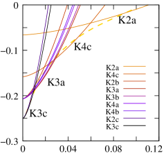
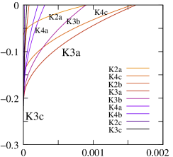
Figure 1: The normalized ground state energy $\frac{E_{\text{tot}}^{K}(n_{e})}{e^{2}\sqrt{n_{e}}/\epsilon}$, minus the normalized ground state energy of quarter Fermi liquid $\frac{E_{\text{tot}}^{\text{QFL}}(n_{e})}{e^{2}\sqrt{n_{e}}/\epsilon}$, is plotted as a function of normalized density $x=n_{e}/\bar{n}_{e}$.
Left: For dispersion $\varepsilon\sim k^{4}$ (i.e. $\gamma=4$) and $x\in[0,0.12]$. The tetralayer graphene at $\gamma=4$ has $\bar{n}_{e}=8.5\times 10^{12}$cm^-2.
Right: For dispersion $\varepsilon\sim k^{2}$ (i.e. $\gamma=2$) and $x\in[0,0.002]$, The tetralayer graphene at $\gamma=2$ has $\bar{n}_{e}=9.8\times 10^{12}$cm^-2.
We see that for $\gamma=4$ case, the chiral superconductivity appears around density $10^{12}$cm^-2 (i.e. have energies less than that of quarter Fermi liquids), while for $\gamma=2$ case, the chiral superconductivity appears around $0.02\times 10^{12}$cm^-2. The Wigner crystal was observed experimentally below $n_{e}\sim 0.5\times 10^{12}$cm^-2.

To plot the energy of the various states as a function of electron density $n_{e}$, it is helpful to measure $E_{\text{tot}}^{K}(n_{e})$ in the unit of $\frac{e^{2}\sqrt{n_{e}}}{\epsilon}$. We find the normalized energy to be

$$\frac{E_{\text{tot}}^{K}(n_{e})}{e^{2}\sqrt{n_{e}}/\epsilon} =V+\frac{\epsilon c_{\gamma}}{e^{2}}(2\pi n_{e})^{(\gamma-1)/2}Z_{\gamma}$$

$$=V+x^{(\gamma-1)/2}Z_{\gamma}$$ (41)

where $x$ describes the total electron density in unit of $\bar{n}_{e}$:

$$n_{e}=x\bar{n}_{e},\ \ \ \bar{n}_{e}=\frac{1}{2\pi}\Big{(}\frac{e^{2}}{\epsilon c_{\gamma}}\Big{)}^{2/(\gamma-1)}$$ (42)

To estimate $\bar{n}_{e}$ for the tetralayer graphene at $\gamma=4$, we use the band dispersion $10$meV $=c_{4}(0.1/a_{0})^{4}$ where $a_{0}=0.246$nm $=4.65a_{B}$, giving $\bar{n}_{e}=8.5\times 10^{12}$ cm^-2. To estimate $\bar{n}_{e}$ for the tetralayer graphene at $\gamma=2$, we use band dispertion $30$meV $=c_{2}(0.1/a_{0})^{2}$, giving $\bar{n}_{e}=9.8\times 10^{12}$ cm^-2.

In Fig. 1, we plot the normalized energy $\frac{E_{\text{tot}}^{K}(n_{e})}{e^{2}\sqrt{n_{e}}/\epsilon}$ (minus that for quarter Fermi liquid) as a function of normalized density $x=n_{e}/\bar{n}_{e}$, for $\gamma=4$ and for $\gamma=2$ cases. We find that for $\gamma=4$ case, the chiral superconductivity appears below a density $n_{e}\sim 10^{12}$cm^-2 (i.e. have energies less than that of quarter Fermi liquid). Experimentally, chiral superconductivity was observed around $n_{e}\sim 0.5\times 10^{12}$cm^-2 and a Wigner crystal was observed below $n_{e}\sim 0.5\times 10^{12}$cm^-2 [15, 38]. Our $\gamma=4$ result fits experimental result very well. For $\gamma=2$ case, the chiral superconductors has energies less than that of quarter Fermi liquid below a density $n_{e}\sim 0.02\times 10^{12}$cm^-2, which do not lead to chiral superconductivity, since at such a low density, Wigner crystal has lower energy. Thus, a flat dispersion is very helpful for chiral superconductivity.

We remark that, for $\gamma=2$ and $\gamma=4$ cases, the energy of $K_{2a}$ chiral superconductor in Fig. 1 is obtained with a fixed wave function described by

$$\bar{K}^{+}=\begin{pmatrix}1&0\\ 0&1\\ \end{pmatrix},\ \ \ \ \bar{K}^{-}=\begin{pmatrix}0&1\\ 1&0\\ \end{pmatrix}$$

At low densities, the energy of $K_{2a}$ chiral superconductor can be lowered further by increasing $\bar{K}^{\pm}$:

$$\bar{K}^{+}=\begin{pmatrix}1+\delta K&\delta K\\ \delta K&1+\delta K\\ \end{pmatrix},\ \bar{K}^{-}=\begin{pmatrix}\delta K&1+\delta K\\ 1+\delta K&\delta K\\ \end{pmatrix}$$

This further minimized energy of $K_{2a}$ chiral superconductor is given by the dashed-curve in Fig. 1. So at low densities, according to our calculation, many different chiral superconductors have similar energies including the $K_{2a}$ chiral superconductor. Further study is needed to determine which one has the lowest energy.

All the superconducting states studied in the paper, $K_{2a}$, $K_{2b}$, etc., break the time-reversal and reflection symmetry in the orbital motion of electrons, and thus carry magnetic moment. The $K_{2a}$, $K_{2b}$, and $K_{2c}$ superconducting states has two spin-valley components with a higher density, and the other two spin-valley components with a lower density. The $K_{4a}$, $K_{4b}$ and $K_{4c}$ superconducting states have all four spin-valley components at equal density. The other superconducting state has one spin-valley component with a highest density, and the other three spin-valley components with lower densities.

Because the densities in different spin-valley components have quantized ratios and is very different between those chiral superconducting states and quarter Fermi liquid, the zero-temperature transition between chiral superconducting states and quarter Fermi liquid is first order. This is a key prediction of this paper.

III Chiral superconductors with non-trivial topological orders

Table 1: Topological properties of the chiral superconductors. The table lists the number $N_{\text{top}}$ of topological excitations (with no $A_{\mu}$-flux i.e. no vorticity), the charge-$e_{SF}$ condensation (which determine the minimal electromagnetic $A_{\mu}$-flux quantum), chiral central charge $c$ (i.e. the number of chiral edge modes), the fractions for each spin-valley components $f_{I}$, the topological Hall response $\sigma=\boldsymbol{e}^{\text{top}\top}(K^{\text{top}})^{-1}\boldsymbol{e}^{\text{top}}$, the average orbital angular momentum $\langle L\rangle$ per electron, and the type of topological order in the topological chiral superconductor.

$K$-matrix	$N_{\text{top}}$	$e_{SF}$	$c$	$f_{I}$	$\sigma$	$\langle L\rangle$	type of topological order
$K_{2a}$ (31)	1	$2$	1	$\frac{1}{2},\frac{1}{2}$	$1$	$-\frac{1}{2}$	$\begin{matrix}\text{$K^{\text{top}}=(1)$},\ \boldsymbol{e}^{\text{top}}=(1)\\[-2.84526pt] \text{``spin''-triplet $p+\hskip 1.0pt\mathrm{i}\hskip 1.0ptp$ superconductor }\\ \end{matrix}$
$K_{2b}$ (32)	3	$2$	1	$\frac{1}{2},\frac{1}{2}$	$\frac{1}{3}$	$-\frac{3}{2}$	$K^{\text{top}}=(3)$, $\boldsymbol{e}^{\text{top}}=(1)$
$K_{2c}$ (33)	5	$2$	1	$\frac{1}{2},\frac{1}{2}$	$\frac{1}{5}$	$-\frac{5}{2}$	$K^{\text{top}}=(5)$, $\boldsymbol{e}^{\text{top}}=(1)$
$K_{3a}$ (34)	1	$4$	0	$\frac{1}{4},\frac{1}{2},\frac{1}{4}$	$0$	$1$	$K^{\text{top}}=\begin{pmatrix}-1&0\\ 0&1\\ \end{pmatrix}$, $\boldsymbol{e}^{\text{top}}=(1,1)$
$K_{3b}$ (35)	1	$6$	0	$\frac{1}{6},\frac{1}{2},\frac{1}{3}$	$-8$	$-1$	$K^{\text{top}}=\begin{pmatrix}-1&0\\ 0&1\\ \end{pmatrix}$, $\boldsymbol{e}^{\text{top}}=(-3,1)$
$K_{3c}$ (36)	10	$4$	0	$\frac{1}{4},\frac{1}{2},\frac{1}{4}$	$-8\frac{1}{5}$	$-1$	$K^{\text{top}}=\begin{pmatrix}-5&0\\ 0&2\\ \end{pmatrix}$, $\boldsymbol{e}^{\text{top}}=(9,4)$
$K_{4a}$ (37)	1	$4$	$-1$	$\frac{1}{4},\frac{1}{4},\frac{1}{4},\frac{1}{4}$	$-25$	$-\frac{1}{2}$	$K^{\text{top}}=\begin{pmatrix}-1&0&0\\ 0&-1&0\\ 0&0&1\\ \end{pmatrix}$, $\boldsymbol{e}^{\text{top}}=(1,7,5)$
$K_{4b}$ (38)	12	$4$	3	$\frac{1}{4},\frac{1}{4},\frac{1}{4},\frac{1}{4}$	$-1$	$-\frac{1}{2}$	$K^{\text{top}}=\begin{pmatrix}-2&0&0\\ 0&3&0\\ 0&0&-2\\ \end{pmatrix}$, $\boldsymbol{e}^{\text{top}}=(2,3,2)$
$K_{4c}$ (39)	1	$4$	-1	$\frac{1}{4},\frac{1}{4},\frac{1}{4},\frac{1}{4}$	$-1$	$\frac{1}{2}$	$K^{\text{top}}=\begin{pmatrix}-1&0&0\\ 0&-1&0\\ 0&0&1\\ \end{pmatrix}$, $\boldsymbol{e}^{\text{top}}=(3,1,3)$

The above chiral superconductors described by (II) usually have non-trivial topological orders and are beyond BCS. We now compute the topological order and other properties of such chiral superconductors. Following Ref. 33, 8, 12, we start with the effective Lagrangian for the chiral superconductor described by (II):

$${\cal L}= \frac{K_{IJ}}{4\pi}a_{I\mu}\partial_{\nu}a_{J\lambda}\epsilon^{\mu\nu\lambda}-\frac{e_{I}}{2\pi}A_{\mu}\partial_{\nu}a_{I\lambda}\epsilon^{\mu\nu\lambda}$$

$$-a_{I0}l_{I}\delta(\boldsymbol{x}),$$

$$\boldsymbol{e}^{\top} =(1,1,\cdots),$$ (43)

where

$$K=\bar{K}^{+}-\bar{K}^{-}$$ (44)

and $J_{\mu}^{I}=\frac{1}{2\pi}\partial_{\nu}a_{I\lambda}\epsilon^{\mu\nu\lambda}$ are the density and current of $I^{\text{th}}$ spin-valley component. The above effective theory is a compact $U(1)$ Chern-Simons theory with integral quantized $U(1)$ charges $l_{I}$. The $K$ has a zero eigenvalue which gives rise to the gapless superfluid mode.

It is convenient to choose an integral basis to make $K$ to have the following block form

$$\widetilde{K}=\begin{pmatrix}K^{\text{top}}&\boldsymbol{0}^{\top}\\ \boldsymbol{0}&0\\ \end{pmatrix}.$$ (45)

Such an integral basis always exists. First $K$ can be written as $K=UDW$, where $U$ and $W$ are unimodular integral matrices, and $D$ is the Smith normal form of $K$, which is a diagonal matrix. Since $K$ has an zero eigenvalue, diagonal of $D$ has a form $(D_{11},D_{22},\cdots,D_{\kappa\kappa}=0)$, where $\kappa$ is the dimension of $K$. Now we introduce $\widetilde{a}_{I\mu}$ via

$$a_{I\mu}=(W^{-1})_{IJ}\widetilde{a}_{J\mu},$$ (46)

and write the effective Lagrangian (III) in terms of $\widetilde{a}_{I\mu}$:

$${\cal L} =\frac{\widetilde{K}_{IJ}}{4\pi}\widetilde{a}_{I\mu}\partial_{\nu}\widetilde{a}_{J\lambda}\epsilon^{\mu\nu\lambda}-\frac{\widetilde{e}_{I}}{2\pi}A_{\mu}\partial_{\nu}\widetilde{a}_{I\lambda}\epsilon^{\mu\nu\lambda}-\widetilde{a}_{I0}\widetilde{l}_{I}\delta(\boldsymbol{x}),$$

$$\widetilde{K} =(W^{\top})^{-1}KW^{-1},\ \widetilde{\boldsymbol{e}}=(W^{\top})^{-1}\boldsymbol{e}=(\boldsymbol{e}^{\text{top}},e_{SF})$$ (47)

We see that

$$\widetilde{K}=(W^{\top})^{-1}UD.$$ (48)

Such a matrix is symmetric and integral. Since $D_{n\kappa}=0$, the last column of $\widetilde{K}$ is zero. The last row of $\widetilde{K}$ is also zero since $\widetilde{K}$ is symmetric.

When there is a gapless mode, we must include Maxwell terms as the new leading order contribution in the superfluid sector. This includes a term $g_{SF}\widetilde{f}_{SF,\mu\nu}\widetilde{f}_{SF}^{\mu\nu}$, where $\widetilde{f}_{SF,\mu\nu}=\partial_{\mu}\widetilde{a}_{SF,\nu}-\partial_{\nu}\widetilde{a}_{SF,\mu}$, and $g_{I}\widetilde{f}_{SF,\mu\nu}\widetilde{f}_{I}^{\mu\nu}$ where $\widetilde{f}_{I,\mu\nu}=\partial_{\mu}\widetilde{a}_{I,\nu}-\partial_{\nu}\widetilde{a}_{I,\mu}$. Writing $\hat{\partial}^{\mu\nu}=\epsilon^{\mu\nu\lambda}\partial_{\lambda}$, the effective Lagrangian (III) becomes

$${\cal L}= \;\widetilde{\boldsymbol{a}}_{\mu}\begin{pmatrix}\tfrac{1}{4\pi}K^{\text{top}}\;\hat{\partial}^{\mu\nu}&\boldsymbol{g}\;{\hat{\partial}^{\mu}}_{\sigma}\hat{\partial}^{\sigma\nu}\\ \boldsymbol{g}^{\top}\;{\hat{\partial}^{\mu}}_{\sigma}\hat{\partial}^{\sigma\nu}&g_{SF}\;{\hat{\partial}^{\mu}}_{\sigma}\hat{\partial}^{\sigma\nu}&\end{pmatrix}\widetilde{\boldsymbol{a}}_{\nu}+\frac{\widetilde{\boldsymbol{e}}}{2\pi}A_{\mu}\hat{\partial}^{\mu\nu}\widetilde{\boldsymbol{a}}_{\nu}$$

$$-\widetilde{\boldsymbol{l}}\cdot\widetilde{\boldsymbol{a}}\;\delta(\boldsymbol{x})$$ (49)

We see that the electron current is given by

$$J^{\mu} =\frac{\widetilde{\boldsymbol{e}}}{2\pi}\cdot\partial_{\nu}\widetilde{\boldsymbol{a}}_{\lambda}\epsilon^{\mu\nu\lambda}.$$ (50)

The gauge field $\widetilde{a}_{SF\mu}$ in the last component of $\widetilde{\boldsymbol{a}}$ is gapless and describes the gapless superfluid mode of the chiral superconductor. The other gauge fields $\widetilde{a}_{I\mu}$ are gapped and describe the topological sector of the chiral superconductor with topological order.

The basis of (45) is not unique, and there is an ambiguity in separating out the superfluid mode. In particular, we can add a multiple of $a_{SF}$ onto any of the topological gauge fields and preserve the form of 45. In the new basis, the $g_{I}$ have changed. Had we included Maxwell terms in the topological sector, a full matrix $g_{\text{tot}}$ would transform under this basis change, but we continue to throw out any mixing of $g_{I}$ into the purely topological sector. Any lowest order terms in our analysis will not be affected by this truncation.

The chiral superconductor behaves like a usual superconductor stacked with a topological sector that may have a non-zero Hall conductance. To understand the responses, we integrate out the dynamical gauge fields. The new Lagrangian describing a purely electromagnetic response is formally

$${\cal L}^{EM}= \;\frac{1}{4}\hat{\partial}^{\mu\lambda}A_{\lambda}\frac{\widetilde{\boldsymbol{e}}^{\top}}{2\pi}M_{\mu\nu}^{-1}\frac{\widetilde{\boldsymbol{e}}}{2\pi}\hat{\partial}^{\nu\rho}A_{\rho}$$ (51)

$$M^{\mu\nu}= \;\begin{pmatrix}\tfrac{1}{4\pi}K^{\text{top}}\;\hat{\partial}^{\mu\nu}+i\epsilon&\boldsymbol{g}\;{\hat{\partial}^{\mu}}_{\sigma}\hat{\partial}^{\sigma\nu}\\ \boldsymbol{g}^{\top}\;{\hat{\partial}^{\mu}}_{\sigma}\hat{\partial}^{\sigma\nu}&g_{SF}\;{\hat{\partial}^{\mu}}_{\sigma}\hat{\partial}^{\sigma\nu}+i\epsilon\end{pmatrix}$$ (52)

where we added an $i\epsilon$ identity term to the quadratic-in-$\widetilde{\boldsymbol{a}}$ term to make the integrals converge. The inverse of $M$ can be written in terms of $g$ and $K$ and their inverses, and these can be expanded order by order in derivatives.

The lowest order term is

$$M_{SF}^{-1}=\begin{pmatrix}0&\boldsymbol{0}^{\top}\\ \boldsymbol{0}&\left(g_{SF}\;{\hat{\partial}^{\mu}}_{\sigma}\hat{\partial}^{\sigma\nu}+i\epsilon\right)^{-1}\end{pmatrix}$$ (53)

Some care must be taken combining the two inverse derivatives with the derivatives on $A_{\mu}$. We work in Lorentz signature $(-,+,+)$, Fourier transform, and fix the gauge to $a_{0}=0$. In a basis $\{\widetilde{a}_{t},\widetilde{a}_{\ell}\}=\{(0,-p_{y},p_{x}),(0,p_{x},p_{y})\}$ labeling the transverse and longitudinal components respectively, we obtain

$$\hat{p}^{\mu\lambda}\left({\hat{p}^{\mu}}_{\sigma}\hat{p}^{\sigma\nu}+i\epsilon\right)^{-1}p^{\nu\rho}=\begin{pmatrix}\frac{\omega^{2}+p_{x}^{2}+p_{y}^{2}}{\omega^{2}+p_{x}^{2}+p_{y}^{2}+i\epsilon}&0\\ 0&\frac{\omega^{2}+p_{x}^{2}+p_{y}^{2}}{\omega^{2}-p_{x}^{2}-p_{y}^{2}+i\epsilon}\end{pmatrix}$$

The term in the transverse component has no pole, so we can take $\epsilon$ to zero and replace it by $1$. The lowest order term in the EM Lagrangian is obtained by contracting this with $A_{t}$ and $A_{\ell}$ in the same basis. Some intuition for this basis can be gained by Fourier transforming back to position space. We have $A_{t}(\boldsymbol{x})=(0,-\partial_{y}\psi_{t},\partial_{x}\psi_{t})$ and $A_{\ell}(\boldsymbol{x})=(0,\partial_{x}\psi_{\ell},\partial_{y}\psi_{\ell})$ where the $\psi$ are scalar functions of position and time. The longitudinal part describes pure electric field due to vanishing curl. The transverse part describes a nonzero background magnetic field if $\nabla^{2}\psi_{t}\neq 0$. Since we are interested in the case of zero magnetic field, we deduce that $\psi_{t}$ is a solution of the Laplace equation.

Returning to momentum space, a general vector potential $\widetilde{A}$ can be separated into longitudinal and transverse parts via the projectors

$$\widetilde{A}_{\ell}^{i}=\frac{p^{i}p_{j}}{p_{x}^{2}+p_{y}^{2}}\widetilde{A}^{j},\quad\widetilde{A}_{t}^{i}=\frac{\epsilon^{i\ell}p_{\ell}\epsilon_{jk}p^{k}}{p_{x}^{2}+p_{y}^{2}}\widetilde{A}^{j}$$ (54)

where we use Latin indices to emphasize that $A$ only has $x$ and $y$ vector potential components and $A_{0}=0$.

We can now write the lowest order part of the EM Lagrangian

$${\cal L}^{EM}_{SF}=\frac{\widetilde{e}_{SF}^{2}}{4(2\pi)^{2}g_{SF}} \left(\widetilde{A}^{\mu}_{t}\widetilde{A}_{t,\mu}+\frac{\omega^{2}+p_{x}^{2}+p_{y}^{2}}{\omega^{2}-p_{x}^{2}-p_{y}^{2}+i\epsilon}\widetilde{A}_{\ell}^{\mu}\widetilde{A}_{\ell,\mu}\right)$$ (55)

The supercurrent is

$$J_{SF}^{\mu} \;=\frac{\widetilde{e}_{SF}^{2}}{2(2\pi)^{2}g_{SF}}\left(\frac{\epsilon^{\mu i}p_{i}\epsilon_{jk}p^{k}}{p_{x}^{2}+p_{y}^{2}}\right.$$

$$+\left.\left(\frac{\omega^{2}+p_{x}^{2}+p_{y}^{2}}{\omega^{2}-p_{x}^{2}-p_{y}^{2}+i\epsilon}\right)\frac{p^{\mu}p_{j}}{p_{x}^{2}+p_{y}^{2}}\right)\widetilde{A}^{j}$$ (56)

This is the London equation for superconductors, where the gauge of $A$ has been fixed by $A_{0}=0$.

The next order contribution to $M^{-1}$ describes the Hall response of the topological sector.

$$M^{-1}_{top}=4\pi\begin{pmatrix}(K^{\text{top}}\hat{\partial}^{\mu\nu}+i\epsilon)^{-1}&\frac{-(K^{\text{top}}\hat{\partial}^{\mu\nu}+i\epsilon)^{-1}\boldsymbol{g}}{g_{SF}}\\ \frac{-\boldsymbol{g}^{\top}(K^{\text{top}}\hat{\partial}^{\mu\nu}+i\epsilon)^{-1}}{g_{SF}}&\frac{\boldsymbol{g}^{\top}(K^{\text{top}}\hat{\partial}^{\mu\nu}+i\epsilon)^{-1}\boldsymbol{g}}{g_{SF}^{2}}\end{pmatrix}$$ (57)

Contracting with $\hat{\partial}^{\mu\nu}A_{\nu}$, factors of $\hat{\partial}^{\mu\nu}$ cancel without poles, so we take $\epsilon$ to zero. We obtain the Chern-Simons factor in the EM Lagrangian

$${\cal L}^{EM}_{top}=\frac{\widetilde{\boldsymbol{e}}^{\top}}{4\pi}\begin{pmatrix}(K^{\text{top}})^{-1}&\frac{-(K^{\text{top}})^{-1}\boldsymbol{g}}{g_{SF}}\\ \frac{-\boldsymbol{g}^{\top}(K^{\text{top}})^{-1}}{g_{SF}}&\frac{\boldsymbol{g}^{\top}(K^{\text{top}})^{-1}\boldsymbol{g}}{g_{SF}^{2}}\end{pmatrix}\widetilde{\boldsymbol{e}}\;\epsilon^{\mu\nu\lambda}A_{\mu}\partial_{\nu}A_{\lambda}$$ (58)

where $\epsilon^{\prime}$ carries a factor of $\hat{p}^{-1}$. From this the Hall response can be written as

$$J_{top}^{\mu}=\frac{\widetilde{\boldsymbol{e}}^{\top}}{2\pi}\begin{pmatrix}(K^{\text{top}})^{-1}&\frac{-(K^{\text{top}})^{-1}\boldsymbol{g}}{g_{SF}}\\ \frac{-\boldsymbol{g}^{\top}(K^{\text{top}})^{-1}}{g_{SF}}&\frac{\boldsymbol{g}^{\top}(K^{\text{top}})^{-1}\boldsymbol{g}}{g_{SF}^{2}}\end{pmatrix}\widetilde{\boldsymbol{e}}\;\epsilon^{\mu\nu\lambda}\partial_{\nu}A_{\lambda}$$ (59)

This term includes $\boldsymbol{g}$, but one can check it is invariant under a basis change redefining the topological sector relative to the superfluid component. In fact, there is such a basis change in which $\boldsymbol{g}=\boldsymbol{0}$, in which case the Hall response reduces to

$$J_{top}^{\mu} =\sigma\epsilon^{\mu\nu\lambda}\partial_{\nu}A_{\lambda}$$

$$\sigma \equiv e_{I}^{\text{top}}(K^{\text{top}})^{-1}_{IJ}e_{J}^{\text{top}}$$ (60)

In this manner, the matrix $g_{\text{tot}}$ acts as a metric on the gauge fields. The basis in which the topological response separates from the superfluid response is the basis in which $\widetilde{a}_{I}g_{\text{tot}}\widetilde{a}_{SF}=0$. This basis may not preserve the vortex quantization, but it does preserve quantization of the Hall response. We can see this explicitly by noting that from a vortex-quantized basis, $\boldsymbol{g}$ becomes zero under the transformation $\widetilde{a}_{I}\rightarrow\widetilde{a}_{I}+t_{I}\widetilde{a}_{SF}$ where $t_{I}=-g_{I}/g_{SF}$. $\widetilde{\boldsymbol{e}}$ transforms as the dual, $\widetilde{e}_{I}\rightarrow\widetilde{e}_{I}$ and $\widetilde{e}_{SF}\rightarrow\widetilde{e}_{SF}+t_{I}\widetilde{e}_{I}$. Since this transformation only affects $\widetilde{e}_{SF}$, it does not change the universal Hall response in III. Thus the total response current is

$$J^{i} \;=\sigma\epsilon^{ij}\omega\widetilde{A}_{j}+\frac{\widetilde{e}_{SF}^{2}}{2(2\pi)^{2}g_{SF}}\left(\frac{\epsilon^{i\ell}p_{\ell}\epsilon_{jk}p^{k}}{p_{x}^{2}+p_{y}^{2}}\right.$$

$$+\left.\left(\frac{\omega^{2}+p_{x}^{2}+p_{y}^{2}}{\omega^{2}-p_{x}^{2}-p_{y}^{2}+i\epsilon}\right)\frac{p^{i}p_{j}}{p_{x}^{2}+p_{y}^{2}}\right)\widetilde{A}^{j}$$ (61)

where $\omega\widetilde{A}_{j}$ is the electric field, and as before we use Latin indices to indicate spatial degrees of freedom. We see that the topological electromagnetic response $\sigma\epsilon^{ij}\omega\widetilde{A}_{j}$ can be separated from other electromagnetic responses, and we can measure the topological Hall conductance $\sigma$ even in the superfluid phase.

To obtain the topological order in the chiral superconductor, we need to study its topological excitations, which are labeled by integer vectors $(\widetilde{l}_{I},\widetilde{l}_{SF})$. The term $-\widetilde{a}_{I0}\widetilde{l}_{I}\delta(\boldsymbol{x})-\widetilde{a}_{SF,0}\widetilde{l}_{SF}\delta(\boldsymbol{x})$ in the effective Lagrangian describes such a topological excitation located at $\boldsymbol{x}=0$. From the equation of motion for $\widetilde{a}_{SF,0}$,

$$-\frac{e_{SF}}{2\pi}\partial_{i}A_{j}\epsilon^{ij}=\widetilde{l}_{SF}\delta(\boldsymbol{x}),$$ (62)

we obtain

$$\frac{1}{2\pi}\partial_{i}A_{j}\epsilon^{ij}=-e_{SF}^{-1}\widetilde{l}_{SF}\delta(\boldsymbol{x}).$$ (63)

We see that if $\widetilde{l}_{SF}\neq 0$, the excitation corresponds to a vortex in the chiral superconductor [8, 12]. Such a vortex carries a $\widetilde{e}_{SF}^{-1}$ unit of $A_{\mu}$-flux:

$$A_{\mu}\text{-flux}=-2\pi e_{SF}^{-1}.$$ (64)

Thus, the chiral superconductor has a charge-$e_{SF}$ condensation.

When $\widetilde{l}_{SF}=0$, the excitations labeled by $\widetilde{\boldsymbol{l}}^{\top}=(\widetilde{l}_{I})$ are finite energy excitations in the chiral superconductor (i.e. not vortices). This kind of excitations has statistics and mutual statistics

$$s_{\widetilde{\boldsymbol{l}}}=\frac{1}{2}\widetilde{\boldsymbol{l}}^{\top}(K^{\text{top}})^{-1}\widetilde{\boldsymbol{l}},\ \ \ \ s_{\widetilde{\boldsymbol{l}},\widetilde{\boldsymbol{l}}^{\prime}}=\widetilde{\boldsymbol{l}}^{\top}(K^{\text{top}})^{-1}\widetilde{\boldsymbol{l}}^{\prime}.$$ (65)

which are fully determined by the $(K^{\text{top}})$-matrix. The $S$ and $T$ matrices are defined as

$$\mathcal{S}_{ij}=\tfrac{1}{\sqrt{N_{\mathrm{top}}}}e^{-2\pi\hskip 1.0pt\mathrm{i}\hskip 1.0pts_{ij}},\quad\mathcal{T}_{ij}=\delta_{ij}e^{\hskip 1.0pt\mathrm{i}\hskip 1.0pt2\pi s_{i}}$$ (66)

which describes the topological order in the chiral superconductors.

Beside the $\mathcal{S},\mathcal{T}$-matrices, there is another topological invariant to describe topological order, which is the chiral central charge $c$, defined as the number of positive eigenvalues minus the number of negative eigenvalues of $K^{\text{top}}$. Physically, the chiral central charge is the number of right-moving edge modes minus the number of left-moving edge modes, which can be measure via thermal Hall conductance [39].

For the $K_{2a}$ chiral superconductor (31), its topological order is described by

$$K^{\text{top}}_{2a} =\begin{pmatrix}1\\ \end{pmatrix},\ \ \text{det}(K^{\text{top}}_{2a})=1,\ \ c=1,$$

$$e_{SF} =2,\ \ \sigma=1,\ \ {\boldsymbol{e}^{\text{top}}}=(1)$$ (67)

Since $\text{det}(K^{\text{top}}_{2a})=1$ and $c=1$, the $K_{2a}$ chiral superconductor is a topological superconductor, that has no bulk anyons (since $\text{det}(K^{\text{top}}_{2a})=1$). The topological nature of the superconductor is characterized by its single chiral edge mode (since $c=1$). Such kind of topological order without non-trivial bulk anyons is called invertible topological order. Since the diagonal of $\widetilde{K}_{2a}$ contains odd integers, the invertible topological order is a fermionic invertible topological order. Such a fermionic invertible topological order is characterized by the chiral centetral charge $c=1$ plus the following $\mathcal{S},\mathcal{T}$-matrices

$$\mathcal{S}_{\text{ferm}}=\frac{1}{\sqrt{2}}\begin{pmatrix}1&1\\ 1&1\end{pmatrix},\quad\mathcal{T}_{\text{ferm}}=\begin{pmatrix}1&0\\ 0&-1\end{pmatrix}$$ (68)

We point out that chiral central charge $c=0$ plus the above $\mathcal{S},\mathcal{T}$-matrices will describe a trivial fermion product state.

$|e_{SF}|=2$ indicates that the superconductor has a charge-2 condensation. Such a chiral superconductor is a BCS “spin”-triplet $p+ip$-wave superconductor.

For the $K_{2b}$ chiral superconductor (32), its topological order is described by

$$K^{\text{top}}_{2b} =\begin{pmatrix}3\\ \end{pmatrix},\ \ \text{det}(K^{\text{top}}_{2a})=3,\ \ c=1,$$

$$e_{SF} =2,\ \ \sigma=\frac{1}{3},\ \ {\boldsymbol{e}^{\text{top}}}=(1)$$ (69)

Since $\text{det}(K^{\text{top}}_{2b})=3$ and $c=1$, the $K_{2b}$ chiral superconductor is a topological superconductor, that has non-trivial bulk anyons. Such a chiral superconductor is a beyond-BCS superconductor. The topological properties of other chiral superconductors are summaries in Table 1.

IV Anyon superconductors

Recently, fractional quantum anomalous Hall (FQAH) states were discovered in Ref. 40, 41, 42. It was usually stressed that FQAH states can appear at a zero magnetic field. Here, we stress that FQAH states are special because they are realized in a periodic potential. If we add electrons/holes to such lattice FQAH states, we will obtain an anyon gas hopping in a background triangle lattice. Such an anyon gas in triangle lattice has been studied in Ref. 12, where anyon superconductivity with intrinsic topological order was discovered. However, Ref. 12 only studied certain possible anyon superconducting states. In this section, we will explore other possible anyon superconducting states which may be simpler. We hope among those possible anyon superconducting states, some of them can be realized in neighborhood of FQAH states, when the periodic potential for anyons is strong enough. As stressed in Ref. 12, the anyon superconductivity near FQAH phases is actually induced by strong Coulomb repulsion, and is a special case of chiral superconductors discussed in the previous sections.

The doped FQAH states are also independently studied in Ref. 43 recently. There, the lattice effects are more explicitly explored, which allows some other states besides the Abelian anyon superfluids to be studied.

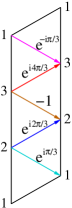
$\begin{matrix}\includegraphics[align=c,height=43.36243pt]{band6min}\\ \\ \includegraphics[align=c,height=43.36243pt]{band3min}\\ \end{matrix}$                     

Figure 2: (left) The magnetic unit cell, where anyons have lowest energy at the site of triangle lattice. The anyon hopping on a triangle lattice has hopping amplitude $-t_{ij}$ whose phase is $0$ on black links, and on colored link as indicated above. The resulting lowest band in the magnetic Brillouin zone is given by the middle-top graph, which has six minima (the black regions between three white regions). (right) The magnetic unit cell, where the anyons have lowest energy at the centers of the triangles. The resulting lowest band has three minimal points (the middle-bottom graph).

Let us consider a filling fraction $\nu=\frac{1}{3}$ FQAH state realized in a 2-dimension material with a moiré pattern. The moiré pattern usually form a triangle lattice. The FQAH state comes from a $\frac{1}{3}$ filled flat Chern band of Chern number $1$. Thus the $\nu=\frac{1}{3}$ FQAH state has an electron density of $\frac{1}{3}$ electron per moiré unit cell.

If we change the electron density, the added electrons will form an anyon gas on the triangle lattice. The fractional statistics of the anyon is $\theta_{a}=\frac{\pi}{3}$. We first assume that the anyons have lower energy at the sites of the triangle lattice and the hopping of the anyons can be described by a tight binding model on triangle lattice.

We note that an electron in the Chern band behaves like a $2\pi$ flux to the anyon. Thus, the tight binding model of anyon hopping contains $\frac{2\pi}{3}$ flux per moiré unit cell, making the hopping amplitudes complex as given by Fig. 2(left). The resulting anyon band is given by Fig. 2(right), which contain six minimal points. Therefore we have six species of anyons at low energies.

If we assume, instead, the anyons have lower energy at the centers of the triangles, we find that the resulting anyon lowest band has three minimal points. In this second case, we have three species of anyons at low energies.

IV.1 Anyon superconductivity for six species of anyons

The six-species case was discussed in Ref. 12, where $\theta_{a}=\frac{\pi}{3}$ anyon is viewed as a fermion attached to $\frac{2\pi}{3}+2\pi=\frac{8\pi}{3}$ flux. The $2\pi\frac{4}{3}$ flux per fermion was then smeared into an uniform effective “magnetic” field. This changes the anyon gas to a fermion gas of six species of fermions with a total filling fraction $\widetilde{\nu}=\frac{3}{4}$. Such a fermion gas can lead to several possible topological superconducting states.

In this paper, we will use a different mean-field approach, which leads to different possible anyon superconducting states. We view the $\theta_{a}=\frac{\pi}{3}$ anyon as a boson attached to $\frac{2\pi}{3}$ flux. We then smear the $2\pi\frac{1}{3}$ flux per boson into an uniform effective “magnetic” field. This changes the anyon gas to a boson gas of six species of bosons with a total filling fraction $\widetilde{\nu}=3$.

To obtain the above results formally, we start with the effective Lagrangian for the $\nu=\frac{1}{3}$ FQH state of electrons

$${\cal L} =\frac{3}{4\pi}\widetilde{a}_{\mu}\partial_{\nu}\widetilde{a}_{\lambda}\epsilon^{\mu\nu\lambda}-\frac{1}{2\pi}A_{\mu}\partial_{\nu}\widetilde{a}_{\lambda}\epsilon^{\mu\nu\lambda}+\hskip 1.0pt\mathrm{i}\hskip 1.0pt\phi^{\dagger}_{I}(\partial_{0}+\hskip 1.0pt\mathrm{i}\hskip 1.0pt\widetilde{a}_{0})\phi_{I}$$

$$-\frac{1}{2m}|(\partial_{i}+\hskip 1.0pt\mathrm{i}\hskip 1.0pt\widetilde{a}_{i})\phi_{I}|^{2}+\text{Coulomb interaction}$$ (70)

where $A_{\mu}$ is the external electromagnetic field, $J_{\mu}=\frac{1}{2\pi}\partial_{\nu}\widetilde{a}_{\lambda}\epsilon^{\mu\nu\lambda}$ is the electron current, and $\phi_{I}$, $I=1,\cdots,6$, are bosonic fields carrying unit of $\widetilde{a}_{\mu}$ charge. Those bosonic fields describe the six species of anyon excitations.

The six species of bosons form a FQH state described by $K$-matrix:

$$\Big{[}\prod_{I=1}^{6}\prod_{i<j}(z_{i}^{I}-z_{j}^{I})^{K_{II}}\prod_{I<J}\prod_{i,j}(z_{i}^{I}-z_{j}^{J})^{K_{IJ}}\Big{]}\hskip 1.0pt\mathrm{e}^{\frac{1}{4}\sum|z_{i}^{I}|^{2}},$$ (71)

where $I,J=1,\cdots,6$ and $K$ is a $6\times 6$ integer matrix with even diagonal elements. Such a $K$-matrix state, plus its parent electron $\nu=\frac{1}{3}$ FQH state, is described by the following total effective theory

$${\cal L}=\frac{3}{4\pi}\widetilde{a}_{\mu}\partial_{\nu}\widetilde{a}_{\lambda}\epsilon^{\mu\nu\lambda}-\frac{1}{2\pi}A_{\mu}\partial_{\nu}\widetilde{a}_{\lambda}\epsilon^{\mu\nu\lambda}-\frac{q_{I}}{2\pi}\widetilde{a}_{\mu}\partial_{\nu}a_{I\lambda}\epsilon^{\mu\nu\lambda}$$

$$+\frac{K_{IJ}}{4\pi}a_{I\mu}\partial_{\nu}a_{J\lambda}\epsilon^{\mu\nu\lambda},\ \ \ \ q_{I}=1,\ \ I,J=1,\cdots,6.$$ (72)

where $\frac{1}{2\pi}\partial_{\nu}\widetilde{a}_{I\lambda}\epsilon^{\mu\nu\lambda}$ is the current of $I^{\text{th}}$ anyons. This effective theory has been discussed before (see (III) and setting $k_{f}=3$), which is the effective theory for anyon superconductor.

There are many $K$-matrices that can give rise to anyon superconductor. To determine which $K$-matrices are more likely, we roughly estimate the energy of each $K$-matrix quantum Hall state. We note that $K_{IJ}$ is the order of zeros in the wave function as a species-$I$ anyon approach a species-$J$ anyon. For the potential energy, we do not have the potential energy fitting for the anyon-anyon interaction. However, we can make a crude ansatz based on the $b/(K_{IJ}+a)$ form we obtained for the electron-electron interactions, given as

$$V_{IJ}=\frac{1}{K_{IJ}+1}$$ (73)

such that $V_{IJ}$ represents the interaction energy between a species-$I$ anyon and a species-$J$ anyon. The core principle of higher order of zeros giving lower Coulomb energy is therefore maintained. Since $\nu_{I}=(K^{-1})_{IJ}q_{J}$ is proportional to the density of the species-$I$ anyons, we can estimate the total energy of a $K$-matrix quantum Hall state as

$$E_{\text{tot}}(K)=\nu_{I}V_{IJ}\nu_{J}$$ (74)

We remark that the kinetic energy of anyons is ignored in the above estimate.

We find a few $K$-matrices whose energies are low and close, and all the species of anyons have non-zero positive densities. The first one is

$$K_{6A} =\begin{pmatrix}0&0&0&0&1&1\\ 0&0&0&1&0&1\\ 0&0&0&1&1&0\\ 0&1&1&0&0&0\\ 1&0&1&0&0&0\\ 1&1&0&0&0&0\\ \end{pmatrix};\ \ \ \text{det}(K_{6A})=-4,$$ (75)

which in fact has the lowest energy. A similar $K$-matrix which also has the lowest energy is

$$K_{6A^{\prime}} =\begin{pmatrix}0&1&1&0&0&0\\ 1&0&1&0&0&0\\ 1&1&0&0&0&0\\ 0&0&0&0&1&1\\ 0&0&0&1&0&1\\ 0&0&0&1&1&0\\ \end{pmatrix};\ \ \ \text{det}(K_{6A^{\prime}})=4.$$ (76)

Other examples of $K$-matrices satisfying the superfluidity conditions with low energy are

$$K_{6B} =\begin{pmatrix}0&0&0&1&2&1\\ 0&0&1&0&0&0\\ 0&1&0&0&0&0\\ 1&0&0&0&2&1\\ 2&0&0&2&0&0\\ 1&0&0&1&0&2\\ \end{pmatrix};\ \ \ \text{det}(K_{6B})=-16,$$ (77)

$$K_{6C} =\begin{pmatrix}0&0&0&2&2&0\\ 0&0&1&0&0&0\\ 0&1&0&0&0&0\\ 2&0&0&0&2&0\\ 2&0&0&2&0&1\\ 0&0&0&0&1&2\\ \end{pmatrix};\ \ \ \text{det}(K_{6C})=-36,$$ (78)

$$K_{6D} =\begin{pmatrix}0&0&0&2&2&0\\ 0&0&1&0&0&0\\ 0&1&0&0&0&0\\ 2&0&0&0&2&0\\ 2&0&0&2&0&0\\ 0&0&0&0&0&4\\ \end{pmatrix};\ \ \ \text{det}(K_{6D})=-64,$$ (79)

$$K_{6E} =\begin{pmatrix}0&0&0&0&2&0\\ 0&0&1&1&0&0\\ 0&1&0&1&0&0\\ 0&1&1&0&0&0\\ 2&0&0&0&0&0\\ 0&0&0&0&0&2\\ \end{pmatrix};\ \ \ \text{det}(K_{6E})=-16.$$ (80)

The sixth $K$-matrix that describes the anyon superconductor is given by

$$K_{6F}=2\delta_{IJ},\ \ \ I,J=1,\cdots,6;\ \ \ \ \text{det}(K_{6F})=64.$$ (81)

Such a $K$-matrix quantum Hall state has a higher energy. Unlike the other anyon superconductors, the above anyon superconductor does not break the permutation symmetry of the six-species of anyons.

IV.2 Anyon superconductivity for three species of anyons

Table 2: Physical properties of the anyon superconductors for 6- and 3-species of anyons. The table lists the number $N_{\text{top}}$ of topological excitations (with no $A_{\mu}$-flux i.e. no vorticity), the minimal $A_{\mu}$-flux quantum, chiral central charge $c$ of the fermionic topological order, the $\mathcal{T}$-matrix, the $\mathcal{S}$-matrix, the anyon densities $\nu_{I}$, the total energy, the type of superconductor. Note that a quasi-particle has $Q_{\boldsymbol{l}}=0$ (i.e. has no vorticity).

$K$-matrix	$N_{\text{top}}$	$A_{\mu}$-flux	$c$	$\mathcal{T}$-matrix	$\mathcal{S}$-matrix	$\nu_{I}$	$E_{\text{tot}}$	type of superconductor
$K_{6A}$ (75)	1	$1/2$	0	1	1	$\frac{1}{2},\frac{1}{2},\frac{1}{2},\frac{1}{2},\frac{1}{2},\frac{1}{2}$	7.50	electron-pair $s$-wave
$K_{6A^{\prime}}$ (76)	1	$1/2$	$-2$	1	1	$\frac{1}{2},\frac{1}{2},\frac{1}{2},\frac{1}{2},\frac{1}{2},\frac{1}{2}$	7.50	electron-pair $g$-wave
$K_{6B}$ (77)	1	$1/4$	0	1	1	$\frac{1}{4},1,1,\frac{1}{4},\frac{1}{4},\frac{1}{4}$	7.60	4-electron condensation
$K_{6C}$ (78)	1	$1/6$	0	1	1	$\frac{1}{6},1,1,\frac{1}{6},\frac{1}{3},\frac{1}{3}$	7.63	6-electron condensation
$K_{6D}$ (79)	4	$1/2$	0	$\mathcal{T}_{\mathbb{Z}_{2}}$ (97)	$\mathcal{S}_{\mathbb{Z}_{2}}$ (97)	$\frac{1}{4},1,1,\frac{1}{4},\frac{1}{4},\frac{1}{4}$	7.70	$\mathbb{Z}_{2}$-topological order
$K_{6E}$ (80)	4	$1/2$	0	$\mathcal{T}_{\text{sem}}\otimes\mathcal{T}_{\text{sem}}$ (96)	$\mathcal{S}_{\text{sem}}\otimes\mathcal{S}_{\text{sem}}$ (96)	$\frac{1}{2},\frac{1}{2},\frac{1}{2},\frac{1}{2},\frac{1}{2},\frac{1}{2}$	7.75	double-semion top. order
$K_{6F}$ (81)	16	$1/2$	6	$\mathcal{T}_{\mathbb{Z}_{2}}\otimes\mathcal{T}_{\mathbb{Z}_{2}}$ (97)	$\mathcal{S}_{\mathbb{Z}_{2}}\otimes\mathcal{S}_{\mathbb{Z}_{2}}$ (97)	$\frac{1}{2},\frac{1}{2},\frac{1}{2},\frac{1}{2},\frac{1}{2},\frac{1}{2}$	8.00	double $\mathbb{Z}_{2}$ top. order
$K_{3A}$ (93)	1	$1/2$	1	1	1	$1,\frac{3}{2},\frac{1}{2}$	2.87	electron-pair $d$-wave
$K_{3B}$ (94)	2	$1/2$	1	$\mathcal{T}_{\text{sem}}$ (96)	$\mathcal{S}_{\text{sem}}$ (96)	$\frac{3}{2},\frac{1}{2},1$	3.33	single-semion top. order
$K_{3C}$ (95)	7	$1/2$	1	$\mathcal{T}_{7}$ (98)	$\mathcal{S}_{7}$ (98)	$\frac{1}{2},1,\frac{3}{2}$	6.34	$K=-\begin{pmatrix}4&3\\ 3&4\end{pmatrix}$

Now, let us consider the case of three species anyon. We may still view the $\frac{\pi}{3}$ anyon as a boson attached to $\frac{2\pi}{3}$ flux. We then smear the $2\pi\frac{1}{3}$ flux per boson into an uniform effective “magnetic” field. This changes the anyon gas to a boson gas of three species of bosons with a total filling fraction $\widetilde{\nu}=3$. Using $3\times 3$ $K$-matrices, we cannot find a $K$-matrix quantum Hall state with non-negative $K^{-1}\boldsymbol{q}$ and $\widetilde{\nu}=\boldsymbol{q}^{\top}K^{-1}\boldsymbol{q}=3$.

We, instead, view the $\frac{\pi}{3}$ anyon as a boson attached to $\frac{2\pi}{3}+4\pi\times\text{integer}$ flux. We then smear the flux per boson into an uniform effective “magnetic” field. This changes the anyon gas to a boson gas of three species of bosons with a total filling fraction $\widetilde{\nu}$. If the bosons form a quantum Hall state described by a $3\times 3$ $K$-matrix, such a state, plus its parent electron $\nu=\frac{1}{3}$ FQH state, is described by the following total effective theory

$${\cal L} =\frac{\widetilde{K}_{mn}}{4\pi}\widetilde{a}_{m\mu}\partial_{\nu}\widetilde{a}_{n\lambda}\epsilon^{\mu\nu\lambda}-\frac{\widetilde{q}_{m}}{2\pi}A_{\mu}\partial_{\nu}\widetilde{a}_{m\lambda}\epsilon^{\mu\nu\lambda}$$

$$\ \ \ \ -\frac{q_{mI}}{2\pi}\widetilde{a}_{m\mu}\partial_{\nu}a_{I\lambda}\epsilon^{\mu\nu\lambda}+\frac{K_{IJ}}{4\pi}a_{I\mu}\partial_{\nu}a_{J\lambda}\epsilon^{\mu\nu\lambda},$$ (82)

where $I,J=1,\cdots,3$, $m,n=1,\cdots,3$, $\frac{1}{2\pi}\partial_{\nu}a_{I\lambda}\epsilon^{\mu\nu\lambda}$ is the current of $I^{\text{th}}$ anyons. The $\widetilde{K}$ and $\widetilde{\boldsymbol{q}}$ are given by

$$\widetilde{K}=\begin{pmatrix}3&0&0\\ 0&0&1\\ 0&1&0\\ \end{pmatrix},\ \ \ \ \widetilde{\boldsymbol{q}}=\begin{pmatrix}1\\ 0\\ 0\\ \end{pmatrix}$$ (83)

that also describe the $\nu=\frac{1}{3}$ parent FQH state of electrons. $q_{mI}$ has a form

$$(q_{mI})=\begin{pmatrix}1&1&1\\ p_{1}&p_{2}&p_{3}\\ p_{4}&p_{5}&p_{6}\\ \end{pmatrix},$$ (84)

where $p_{1},\cdots,p_{6}$ are integers, describing different ways of attaching $4\pi$ flux to bosons. The total effective theory is described by a total $K$-matrix

$$K_{\text{tot}}=\begin{pmatrix}\widetilde{K}&-(q_{mI})\\ -(q_{mI})^{\top}&K\\ \end{pmatrix}.$$ (85)

From the equation of motion $\partial{\cal L}/\partial a_{m0}=\partial{\cal L}/\partial\widetilde{a}_{I0}=0$:

$$\frac{\widetilde{K}_{mn}}{2\pi}\partial_{i}\widetilde{a}_{nj}\epsilon^{ij} =\frac{\widetilde{q}_{m}}{2\pi}\partial_{i}A_{j}\epsilon^{ij}+\frac{q_{mI}}{2\pi}\partial_{i}a_{Ij}\epsilon^{ij}$$

$$\frac{q_{mI}}{2\pi}\partial_{i}\widetilde{a}_{mj}\epsilon^{ij} =\frac{K_{IJ}}{2\pi}\partial_{i}a_{Jj}\epsilon^{ij}.$$ (86)

The above two equations implies that

$$\frac{\widetilde{K}_{mn}-q_{mI}(K^{-1})_{IJ}q_{nJ}}{2\pi}\partial_{i}\widetilde{a}_{nj}\epsilon^{ij} =\frac{\widetilde{q}_{m}}{2\pi}\partial_{i}A_{j}\epsilon^{ij},$$ (87)

$$\frac{K_{IJ}-q_{mI}(\widetilde{K}^{-1})_{mn}q_{nJ}}{2\pi}\partial_{i}a_{Jj}\epsilon^{ij} =\frac{q_{mI}(\widetilde{K}^{-1}\widetilde{\boldsymbol{q}})_{m}}{2\pi}\partial_{i}A_{j}\epsilon^{ij},$$

which relates the electron density $\frac{1}{2\pi}\partial_{i}\widetilde{a}_{1j}\epsilon^{ij}$ to the magnetic field $B=\partial_{i}A_{j}\epsilon^{ij}$. If the above equation can be satisfied by a finite electron density even for zero magnetic field $B=0$, then the effective Lagrangian (IV.2) describes an anyon superconductor, i.e. an electron superconducting state. This is realized by $K$ and $q_{mI}$ such that

$$\widetilde{\Lambda}_{mn}=\widetilde{K}_{mn}-q_{mI}(K^{-1})_{IJ}q_{nJ}.$$ (88)

has a zero eigenvalue and the corresponding eigenvector $\widetilde{v}_{m}$ has a non-zero 1st component $\widetilde{v}_{1}\neq 0$, and such that

$$\Lambda_{IJ}=K_{IJ}-q_{mI}(\widetilde{K}^{-1})_{mn}q_{nJ}.$$ (89)

has a zero eigenvalue and the components of the corresponding eigenvector $f_{I}$ are all non-zero and have the same sign: $f_{I}>0$. Note that $f_{I}$ is proportional to the density of $I^{\text{th}}$ anyons. The second requirement corresponds to all three species of anyons having positive densities. Note that the electron density is given by

$$n_{e}=\frac{\partial_{i}\widetilde{a}_{1j}\epsilon^{ij}}{2\pi} =\frac{(\widetilde{K}^{-1})_{1m}q_{mI}}{2\pi}\partial_{i}a_{Ij}\epsilon^{ij}=(\widetilde{K}^{-1})_{1m}q_{mI}\rho f_{I}$$

where $\rho f_{I}$ is the density of $I^{\text{th}}$ anyons. Thus we also require that

$$\rho_{e}=(\widetilde{K}^{-1})_{1m}q_{mI}\rho f_{I}>0.$$ (90)

From the above, we find that

$$\rho=\frac{n_{e}}{(\widetilde{K}^{-1})_{1m}q_{mI}f_{I}}$$ (91)

Thus the anyon density is given by (in the unit of $n_{e}$)

$$\nu_{I}=\frac{f_{I}}{(\widetilde{K}^{-1})_{1m}q_{mI}f_{I}}>0.$$ (92)

This allows us to estimate the energy of anyon superconductor via (74).

There are many $K,\ (q_{mI})$ pairs that satisfy the above conditions. The first one with lowest energy is given by

$$K_{3A}=\begin{pmatrix}2&3&1\\ 3&2&2\\ 1&2&6\\ \end{pmatrix},\ \ \ (q_{mI})_{3A}=\begin{pmatrix}1&1&1\\ 1&1&1\\ 1&1&1\\ \end{pmatrix}$$ (93)

The above choice of $(q_{mI})_{3a}$ corresponds to viewing the $\frac{\pi}{3}$ anyon as a boson attached to $\frac{2\pi}{3}+4\pi$ flux. We then smear the flux $2\pi\frac{7}{3}$ per boson into an uniform effective “magnetic” field. This changes the anyon gas to a boson gas of three species of bosons with a total filling fraction $\widetilde{\nu}=\frac{3}{7}$. Such a boson gas can form a $\widetilde{\nu}=\frac{3}{7}$ quantum Hall state described by the above $K$-matrix.

Other examples include

$$K_{3B}=\begin{pmatrix}2&4&2\\ 4&2&0\\ 2&0&4\\ \end{pmatrix};\ \ \ (q_{mI})_{3B}=\begin{pmatrix}1&1&1\\ 1&1&1\\ 1&1&1\\ \end{pmatrix},$$ (94)

and

$$K_{3C}=\begin{pmatrix}0&6&0\\ 6&0&0\\ 0&0&4\\ \end{pmatrix};\ \ \ (q_{mI})_{3C}=\begin{pmatrix}1&1&1\\ 1&0&1\\ 1&1&1\\ \end{pmatrix}.$$ (95)

IV.3 Physical properties of anyon superconducting state

As discussed above, both six-anyon superconductors and three-anyon superconductors are described by effective theory (III), with $K_{\text{tot}}$ given in the previous two subsections. Using such an effective theory, we can calculate the topological order in the anyon superconductors.

The form of the $K$-matrix indicates that the gapped modes belong to an Abelian fermionic topological order. We extract out the intrinsic bosonic topological order by factoring out the trivial fermions so that the $S$ and $T$ matrices satisfy the modular relations $(ST)^{3}=e^{i\pi c/4}S^{2}$ obeyed by the bosonic topological orders. The 3- and 6-species $K$-matrices produce topological orders (both singly and stacked) characterized by

$$\mathcal{S}_{\text{sem}}=\frac{1}{\sqrt{2}}\begin{pmatrix}1&1\\ 1&-1\end{pmatrix},\quad\mathcal{T}_{\text{sem}}=\frac{1}{\sqrt{2}}\begin{pmatrix}1&0\\ 0&i\end{pmatrix}$$ (96)

$$\mathcal{S}_{\mathbb{Z}_{2}}=\frac{1}{2}\begin{pmatrix}1&1&1&1\\ 1&1&-1&-1\\ 1&-1&1&-1\\ 1&-1&-1&1\end{pmatrix},\quad\mathcal{T}_{\mathbb{Z}_{2}}=\begin{pmatrix}1&0&0&0\\ 0&1&0&0\\ 0&0&1&0\\ 0&0&0&-1\end{pmatrix}$$ (97)

$$\mathcal{S}_{7}=\frac{1}{\sqrt{7}}\exp\left(-8ab\pi\hskip 1.0pt\mathrm{i}\hskip 1.0pt/7\right),\ \ \ \mathcal{T}_{7}=\delta_{ab}\exp\left(4a^{2}\pi\hskip 1.0pt\mathrm{i}\hskip 1.0pt/7\right)$$ (98)

The modular relations between $S$ and $T$ matrices then gives the chiral central charge of the bosonic TO, and we have obtained the full modular data of the topological order. Note that the original fermionic TO only provides the chiral central charge to $\text{mod-}1/2$ [44], but the decomposed bosonic TO is defined $\text{mod-}8$. The above results are summarized in Table 2, along with the bosonic $K$-matrices corresponding to the $S$ and $T$ matrices given. As in the previous case in Table 1, we find possible superfluid states with $4e$ and $6e$ condensations, manifested by its vortex quantization.

V Summary

Electron gas in 2-dimension with strong Coulomb interaction will form a Wigner crystal below a critical density. In this paper, we use Laughlin-type wave functions (II) to construct many chiral superconducting states. In light of the experimental finding,[15] we find that, if the electron has a flat dispersion $\varepsilon=c_{4}k^{4}$ and only for such kinds of flat dispersion, some of the chiral superconducting states may have lower energy then Wigner crystal near the critical density.

This is because chiral superconductors have larger momentum fluctuations and larger inter-particle separation compared to the fully spin-valley polarized Fermi liquid. Thus, the topological chiral superconductors are favored when the electron band bottom is very flat. In this limit, the Wigner crystal phase may also be favored. According to our estimate, we find that chiral superconductors have energies close to that of fully spin-valley polarized Fermi liquid and Wigner crystal. Therefore, chiral superconductors, if they do appear, are more likely to appear near the transition between fully spin-valley polarized Fermi liquid and Wigner crystal. All these phases are driven by strong repulsive interaction; this is why the experimentally observed superconducting phase [15] between fully spin-valley polarized Fermi liquid phase and Wigner crystal phase may be a topological chiral superconductor discussed in this paper.

The low energy effective theory of those superconducting states is derived, which is used to compute the properties of their corresponding superconducting states. We find that chiral superconducting states carry non-trivial topological order and are usually not in the same phase with any BCS superconductors. Namely, they often have charge-4 or higher condensation and gapless chiral edge modes.

Certainly, a chiral superconductor induced by pairing instability of the quarter Fermi liquid is also possible, if there is an effective attractive interaction. The chiral superconductors induced by Coulomb repulsion have an energy scale $0.1e^{2}n_{e}^{1/2}/\epsilon$, which is about $2$meV. Compared to this, the observed superconducting state [15] has a transition temperature about $0.3$K. Such a low transition temperature may be due to the strong $U(1)$ phase fluctuations. The time reversal symmetry breaking in correlated electron orbital motion of chiral superconductors should persist beyond the superconducting transition temperature.

The topological chiral superconductors have many characters that are very different from a BCS superconductor. A beyond-BCS topological superconductor will be a very interesting discovery. The large energy scale of the Coulomb interaction $0.1e^{2}\bar{n}_{e}^{1/2}/\epsilon=0.04\Big{(}\frac{e^{2}}{\epsilon}\Big{)}^{4/3}\frac{1}{c_{4}^{1/3}}$ for such chiral superconductivity suggests a direction to obtain high temperature superconductivity.

We would like to thank Xiaodong Xu for helpful discussions last year which motivated the anyon-superconducter part of the work. This work was partially supported by NSF grant DMR-2022428 and by the Simons Collaboration on Ultra-Quantum Matter, which is a grant from the Simons Foundation (651446, XGW). LJ acknowledges the support from a Sloan Fellowship. AT was supported by NSF Graduate Research Fellowship grant number 2141064. Some of the numerical calculations were done on subMIT HPC cluster at MIT.

Appendix A Computations of kinetic and interaction energies

In this section, we calculate the kinetic energy and interaction energy of the wave function (II) of chiral superconductor. To calculate kinetic energy, we first compute the equal-time correlation function for a $I_{0}^{\text{th}}$ species of particle

$$\ \ \ \ G_{I_{0}}(z^{I_{0}},z^{I_{0}*},\widetilde{z}^{I_{0}},\widetilde{z}^{I_{0}*})$$

$$=\int\prod_{I,i}\hskip 1.0pt\mathrm{d}^{2}z_{i}^{I}\Psi^{*}(\widetilde{z}^{I_{0}},\{z_{i}^{I})\}\Psi(z^{I_{0}},\{z_{i}^{I}\})$$

$$=\int\prod_{I,i}\hskip 1.0pt\mathrm{d}^{2}z_{i}^{I}{\cal N}\hskip 1.0pt\mathrm{e}^{-\sum_{i,I}\frac{|z_{i}^{I}|^{2}}{2l_{I}^{2}}}\hskip 1.0pt\mathrm{e}^{-\frac{|z|^{2}}{4l_{I_{0}}^{2}}}\hskip 1.0pt\mathrm{e}^{-\frac{|\widetilde{z}|^{2}}{4l_{I_{0}}^{2}}}$$

$$\ \ \ \ \prod_{i<j,I}|z_{i}^{I}-z_{j}^{I}|^{2\bar{K}_{II}}\prod_{i,j,I<J}|z_{i}^{I}-z_{j}^{J}|^{2\bar{K}_{IJ}}$$

$$\ \ \ \ \prod_{i}(z^{I_{0}}-z_{i}^{I_{0}})^{\bar{K}_{I_{0}I_{0}}^{+}}\prod_{i,I}(z^{I_{0}}-z_{i}^{I})^{\bar{K}_{I_{0}I}^{+}}$$

$$\ \ \ \ \prod_{i}(z^{I_{0}*}-z_{i}^{{I_{0}}*})^{\bar{K}_{I_{0}I_{0}}^{-}}\prod_{i,I}(z^{I_{0}*}-z_{i}^{I*})^{\bar{K}_{I_{0}I}^{-}}$$

$$\ \ \ \ \prod_{i}(\widetilde{z}^{I_{0}*}-z_{i}^{{I_{0}}*})^{\bar{K}_{I_{0}I_{0}}^{+}}\prod_{i,I}(\widetilde{z}^{I_{0}*}-z_{i}^{I*})^{\bar{K}_{I_{0}I}^{+}}$$

$$\ \ \ \ \prod_{i}(\widetilde{z}^{I_{0}}-z_{i}^{{I_{0}}})^{\bar{K}_{I_{0}I_{0}}^{-}}\prod_{i,I}(\widetilde{z}^{I_{0}}-z_{i}^{I})^{\bar{K}_{I_{0}I}^{-}}$$ (99)

where ${\cal N}$ is the normalization coefficient and

$$\bar{K}_{IJ}=\bar{K}_{IJ}^{+}+\bar{K}_{IJ}^{-}$$ (100)

The above integral has sign changes, and it is hard to evaluate it via Monte Carlo method. In the following, we convert the integral into to one that has no sign changes, via holomorphic extension. Let us consider a related function

$$\ \ \ \ \widetilde{G}_{I_{0}}(z_{1},z_{2}^{*},z_{3},z_{4}^{*})$$

$$=\int\prod_{I,i}\hskip 1.0pt\mathrm{d}^{2}z_{i}^{I}\hskip 1.0pt\mathrm{e}^{-\sum_{i,I}\frac{|z_{i}^{I}|^{2}}{2l_{I}^{2}}}$$

$$\ \ \ \ \prod_{i<j,I}|z_{i}^{I}-z_{j}^{I}|^{2\bar{K}_{II}}\prod_{i,j,I<J}|z_{i}^{I}-z_{j}^{J}|^{2\bar{K}_{IJ}}$$

$$\ \ \ \ \prod_{i}(z_{1}-z_{i}^{I_{0}})^{\bar{K}_{I_{0}I_{0}}^{+}}\prod_{i,I}(z_{1}-z_{i}^{I})^{\bar{K}_{I_{0}I}^{+}}$$

$$\ \ \ \ \prod_{i}(z_{2}^{*}-z_{i}^{{I_{0}}*})^{\bar{K}_{I_{0}I_{0}}^{-}}\prod_{i,I}(z_{2}^{*}-z_{i}^{I*})^{\bar{K}_{I_{0}I}^{-}}$$

$$\ \ \ \ \prod_{i}(z_{4}^{*}-z_{i}^{{I_{0}}*})^{\bar{K}_{I_{0}I_{0}}^{+}}\prod_{i,I}(z_{4}^{*}-z_{i}^{I*})^{\bar{K}_{I_{0}I}^{+}}$$

$$\ \ \ \ \prod_{i}(z_{3}-z_{i}^{{I_{0}}})^{\bar{K}_{I_{0}I_{0}}^{-}}\prod_{i,I}(z_{3}-z_{i}^{I})^{\bar{K}_{I_{0}I}^{-}}$$ (101)

We note that $\widetilde{G}_{I_{0}}(z_{1},z_{2}^{*},z_{3},z_{4}^{*})$ is a holomorphic function of $z_{1},z_{3}$ and an anti-holomorphic function of $z_{2},z_{4}$. Such a function can be determined by its values on the subspace $z_{1}=z_{4}$ and $z_{2}=z_{3}$.

$$\ \ \ \ \widetilde{G}_{I_{0}}(z_{1},z_{2}^{*},z_{2},z_{1}^{*})$$

$$=\int\prod_{I,i}\hskip 1.0pt\mathrm{d}^{2}z_{i}^{I}\hskip 1.0pt\mathrm{e}^{-\sum_{i,I}\frac{|z_{i}^{I}|^{2}}{2l_{I}^{2}}}$$

$$\ \ \ \ \prod_{i<j,I}|z_{i}^{I}-z_{j}^{I}|^{2\bar{K}_{II}}\prod_{i,j,I<J}|z_{i}^{I}-z_{j}^{J}|^{2\bar{K}_{IJ}}$$

$$\ \ \ \ \prod_{i}|z_{1}-z_{i}^{I_{0}}|^{2\bar{K}_{I_{0}I_{0}}^{+}}\prod_{i,I}|z_{1}-z_{i}^{I}|^{2\bar{K}_{I_{0}I}^{+}}$$

$$\ \ \ \ \prod_{i}|z_{2}-z_{i}^{I_{0}}|^{2\bar{K}_{I_{0}I_{0}}^{-}}\prod_{i,I}|z_{2}-z_{i}^{I}|^{2\bar{K}_{I_{0}I}^{-}}$$

$$=\int\prod_{I,i}\hskip 1.0pt\mathrm{d}^{2}z_{i}^{I}\hskip 1.0pt\mathrm{e}^{-\sum_{i,I}\frac{|z_{i}^{I}|^{2}}{2l_{I}^{2}}}$$

$$\ \ \ \ \hskip 1.0pt\mathrm{e}^{\sum_{i<j,I}2\bar{K}_{II}\log|z_{i}^{I}-z_{j}^{I}|}\hskip 1.0pt\mathrm{e}^{\sum_{i,j,I<J}2\bar{K}_{IJ}\log|z_{i}^{I}-z_{j}^{J}|}$$

$$\ \ \ \ \hskip 1.0pt\mathrm{e}^{\sum_{i}2\bar{K}_{I_{0}I_{0}}^{+}\log|z_{1}-z_{i}^{I_{0}}|}\hskip 1.0pt\mathrm{e}^{\sum_{i,I}2\bar{K}_{I_{0}I}^{+}\log|z_{1}-z_{i}^{I}|}$$

$$\ \ \ \ \hskip 1.0pt\mathrm{e}^{\sum_{i}2\bar{K}_{I_{0}I_{0}}^{-}\log|z_{2}-z_{i}^{I_{0}}|}\hskip 1.0pt\mathrm{e}^{\sum_{i,I}2\bar{K}_{I_{0}I}^{-}\log|z_{2}-z_{i}^{I}|}$$ (102)

Since $(\bar{K}_{IJ})$ is a positive definite matrix, it can be written as

$$2\bar{K}_{IJ}=\sum_{a=1}^{\text{dim}(\bar{K})}q_{I}^{a}q_{J}^{a}$$ (103)

via Cholesky decomposition. Here we assume the $\bar{K}$ is invertible. If it is not, we can shift $\bar{K}^{+}$ $\bar{K}^{-}$ by a small positive matrix to make $\bar{K}$ invertible. Now we can rewrite

$$-2\bar{K}_{IJ}\log|z^{I}-z^{J}|=-q_{I}^{a}q_{J}^{a}\log|z^{I}-z^{J}|,$$ (104)

which can be viewed as the 2-dimensional Coulomb interaction energy between two charged particles at $z^{I}$ and $z^{J}$. Each charged particle carries $\text{dim}(\bar{K})$ types of charges, labeled by $a$. The $I$-particle carries type-$a$ charge $q_{I}^{a}$ and the $J$-particle carries type-$a$ charge $q_{J}^{a}$.

Therefore, part of $\widetilde{G}_{I_{0}}(z_{1},z_{2}^{*},z_{2},z_{1}^{*})$,

$$Z =\int\prod_{I,i}\hskip 1.0pt\mathrm{d}^{2}z_{i}^{I}\hskip 1.0pt\mathrm{e}^{-\sum_{i,I}\frac{|z_{i}^{I}|^{2}}{2l_{I}^{2}}}$$

$$\ \ \ \ \prod_{i<j,I}|z_{i}^{I}-z_{j}^{I}|^{2\bar{K}_{II}}\prod_{i,j,I<J}|z_{i}^{I}-z_{j}^{J}|^{2\bar{K}_{IJ}}$$ (105)

is the partition function of the above Coulomb gas at temperature $T=1$. The term $\frac{|z_{i}^{I}|^{2}}{2l_{I}^{2}}$ represents the potential energy of a species-$I$ particle produced by an uniform background charge. We note that a background charge density $\rho=-\frac{1}{2\pi}$ will produce a potential $\frac{|z_{i}^{I}|^{2}}{4}$. Therefore, the background charge density $\rho_{a}$ must satisfy

$$\frac{|z_{i}^{I}|^{2}}{2l_{I}^{2}}=\sum_{a}-2\pi\rho_{a}\frac{|z_{i}^{I}|^{2}}{4}q_{I}^{a}\ \ \to\ \ \rho_{a}=-\sum_{I}\widetilde{q}_{I}^{a}\frac{1}{\pi l_{I}^{2}}$$ (106)

where the matrix $(\widetilde{q}_{a}^{I})$ is the inverse of the matrix $(q^{a}_{I})$:

$$\sum_{I}q^{a}_{I}\widetilde{q}_{b}^{I}=\delta_{ab}.$$ (107)

The relative densities $n_{I}$ of species-$I$ particles are fixed by filling fractions of the effective flux via $\sum_{J}K_{IJ}n_{J}=0$. One way to see this is by requiring the kinetic energy to scale linearly in particle number in zero background magnetic field. The total angular momentum at $N^{2}$ order is given by

$$\frac{1}{2}\sum_{IJ}(N_{I}\bar{K}_{IJ}^{+}N_{J}-N_{I}\bar{K}_{IJ}^{-}N_{J})$$ (108)

If we change $N_{I}$ by 1, the change of total angular momentum is given by

$$\sum_{J}(\bar{K}_{IJ}^{+}N_{J}-\bar{K}_{IJ}^{-}N_{J})$$ (109)

Thus, we require

$$\sum_{J}(\bar{K}_{IJ}^{+}N_{J}-\bar{K}_{IJ}^{-}N_{J})=0$$ (110)

in order for the kinetic energy to be finite. This is also the species ratio of the superfluid mode, which is why it persists at zero external magnetic field.

We can now determine the background charge densities $\rho_{a}$. The charge neutrality condition of the Coulomb gas gives

$$\sum_{I}n_{I}q_{I}^{a}+\rho_{a}=0.$$ (111)

This equivalently determines the inter-particle spacing parameters $l_{J}$

$$\sum_{I,a}n_{I}q_{I}^{a}q_{J}^{a} =-\sum_{a}\rho_{a}q_{J}^{a}=\frac{1}{\pi l_{J}^{2}}$$

We see that

$$\sum_{J}\bar{K}_{IJ}n_{J}=\frac{1}{2\pi l_{J}^{2}}.$$ (112)

which is also the condition fixing the size of each species droplet. The maximal power of $|z|$ is given by $\sum_{J}\bar{K}_{IJ}N_{J}$, and the most probable radius occupied by this orbital is

$$R^{2}=2l_{I}^{2}\sum_{J}\bar{K}_{IJ}N_{J}$$

reproducing 112. If $\bar{K}$ is invertible, we can now express the densities using

$$n_{I}=\sum_{J}\frac{(\bar{K}^{-1})_{IJ}}{2\pi l_{J}^{2}}.$$ (113)

If $\bar{K}$ is non-invertible, we cannot readily express $n_{I}$ in terms of the $l_{I}^{-1}$. However, we must remember that $n_{I}$ are the parameters fixed topologically by $K$, and in contrast $l_{I}$ and $\bar{K}$ adjust to minimize energy while keeping these densities fixed. Since $\bar{K}_{IJ}$ controls the order of zero between species, we expect the value which minimizes energy to depend on $n_{I}$ and $n_{J}$, so $\bar{K}_{IJ}=g(n_{I},n_{J})$. If $\bar{K}$ is non-invertible, this means that one row of $\bar{K}$ is linearly dependent on the other rows. We have

$$g(n_{I},n_{J})=\sum_{K}c_{K}g(n_{K},n_{J})$$

Further assuming $g$ is separable into $g(n_{I})g(n_{J})$, we can then extract a relation $n_{I}=g^{-1}\left(\sum_{K}c_{K}g(n_{K})\right)$. This is to say that a density may usually be determined from the others if an inter-particle distance can be determined from the others, and therefore a pseudo-inverse of $\bar{K}$ may be defined. In many cases, $\bar{K}$ fails to be invertible because all densities are the same, and therefore all entries $\bar{K}_{IJ}$ are the same and all $l_{I}$ are also the same. In this case, we can use a matrix proportional to the identity to relate $n_{I}$ and $l_{J}^{-1}$

The term $-2\bar{K}_{I_{0}I}^{+}\log|z_{1}-z_{i}^{I}|$ can also be viewed as a Coulomb energy between the $z_{1}$-particle and a species-$I$ particle if we assume the $z_{1}$-particle carries charge $q_{+}^{a}$, which satisfies

$$2\bar{K}_{I_{0}I}^{+}=\sum_{a}q_{+}^{a}q_{I}^{a}\ \ \to\ \ q_{+}^{a}=\sum_{I}2\bar{K}_{I_{0}I}^{+}\widetilde{q}^{I}_{a}.$$ (114)

Similarly, the term $-2\bar{K}_{I_{0}I}^{-}\log|z_{2}-z_{i}^{I}|$ can be viewed as a Coulomb energy between $z_{2}$-particle and a species-$I$ particle if we assume the $z_{2}$-particle carries charge $q_{-}^{a}$, which satisfies

$$2\bar{K}_{I_{0}I}^{-}=\sum_{a}q_{-}^{a}q_{I}^{a}\ \ \to\ \ q_{-}^{a}=\sum_{I}2\bar{K}_{I_{0}I}^{-}\widetilde{q}^{I}_{a}.$$ (115)

Therefore, the following is the partition function of the Coulomb gas with two extra charged particles, $z_{1}$ and $z_{2}$, present:

$$\ \ \ \ \widetilde{G}_{I_{0}}(z_{1},z_{2}^{*},z_{2},z_{1}^{*})\hskip 1.0pt\mathrm{e}^{-\frac{|z_{1}|^{2}}{4}\sum_{a}-2\pi\rho_{a}q_{+}^{a}-\frac{|z_{2}|^{2}}{4}\sum_{a}-2\pi\rho_{a}q_{-}^{a}}$$

$$=\int\prod_{I,i}\hskip 1.0pt\mathrm{d}^{2}z_{i}^{I}\hskip 1.0pt\mathrm{e}^{-\sum_{i,I}\frac{|z_{i}^{I}|^{2}}{2l_{I}^{2}}}\hskip 1.0pt\mathrm{e}^{\frac{\pi|z_{1}|^{2}}{2}\sum_{a}\rho_{a}q_{+}^{a}+\frac{\pi|z_{2}|^{2}}{2}\sum_{a}\rho_{a}q_{-}^{a}}$$

$$\ \ \ \ \hskip 1.0pt\mathrm{e}^{\sum_{i<j,I}2\bar{K}_{II}\log|z_{i}^{I}-z_{j}^{I}|}\hskip 1.0pt\mathrm{e}^{\sum_{i,j,I<J}2\bar{K}_{IJ}\log|z_{i}^{I}-z_{j}^{J}|}$$

$$\ \ \ \ \hskip 1.0pt\mathrm{e}^{\sum_{i}2\bar{K}_{I_{0}I_{0}}^{+}\log|z_{1}-z_{i}^{I_{0}}|}\hskip 1.0pt\mathrm{e}^{\sum_{i,I}2\bar{K}_{I_{0}I}^{+}\log|z_{1}-z_{i}^{I}|}$$

$$\ \ \ \ \hskip 1.0pt\mathrm{e}^{\sum_{i}2\bar{K}_{I_{0}I_{0}}^{-}\log|z_{2}-z_{i}^{I_{0}}|}\hskip 1.0pt\mathrm{e}^{\sum_{i,I}2\bar{K}_{I_{0}I}^{-}\log|z_{2}-z_{i}^{I}|}.$$ (116)

the term

$$\ \ \ \ -\frac{\pi|z_{1}|^{2}}{2}\sum_{a}\rho_{a}q_{+}^{a}-\frac{\pi|z_{2}|^{2}}{2}\sum_{a}\rho_{a}q_{-}^{a}$$

$$=|z_{1}|^{2}\sum_{I,J}\frac{1}{2l_{I}^{2}}(\bar{K}^{-1})_{IJ}\bar{K}_{I_{0}J}^{+}+|z_{2}|^{2}\sum_{I,J}\frac{1}{2l_{I}^{2}}(\bar{K}^{-1})_{IJ}\bar{K}_{I_{0}J}^{-}$$

$$=|z_{1}|^{2}\sum_{J}\pi n_{J}\bar{K}_{I_{0}J}^{+}+|z_{2}|^{2}\sum_{J}\pi n_{J}\bar{K}_{I_{0}J}^{-}$$ (117)

is the interaction energy between $z_{1,2}$-particle and the background charge. In the above we have used

$$\sum_{a}-\rho_{a}q_{+}^{a} =\sum_{a,I,J}\widetilde{q}_{a}^{I}\frac{1}{\pi l_{I}^{2}}2\bar{K}_{I_{0}J}^{+}\widetilde{q}^{J}_{a}=\sum_{I,J}\frac{1}{\pi l_{I}^{2}}(\bar{K}^{-1})_{IJ}\bar{K}_{I_{0}J}^{+}$$ (118)

We remark that the direct interaction energy between $z_{1}$- and $z_{2}$-particles,

$$-\sum_{a}q_{+}^{a}q_{-}^{a}\log|z_{2}-z_{1}|,$$ (119)

is not included.

If $\bar{K}_{IJ}$ is not too large, the Coulomb gas is in the plasma phase. Due to the perfect screening of the plasma phase, the partition function $\widetilde{G}_{I_{0}}(z_{1},z_{2}^{*},z_{2},z_{1}^{*})\hskip 1.0pt\mathrm{e}^{-\frac{|z_{1}|^{2}}{4}\sum_{a}-2\pi\rho_{a}q_{+}^{a}-\frac{|z_{2}|^{2}}{4}\sum_{a}-2\pi\rho_{a}q_{-}^{a}}$ only depend on the difference of the positions $z_{1}-z_{2}$ of the added charges, if $z_{1},z_{2}$ are in the plasma droplet of radius $R$. Therefore

$$\widetilde{G}_{I_{0}}(z_{1},z_{2}^{*},z_{2},z_{1}^{*}) =g(|z_{1}-z_{2}|)$$

$$\ \ \ \ \hskip 1.0pt\mathrm{e}^{\frac{|z_{1}|^{2}}{4}\sum_{a}-2\pi\rho_{a}q_{+}^{a}+\frac{|z_{2}|^{2}}{4}\sum_{a}-2\pi\rho_{a}q_{-}^{a}}$$

When $|z_{2}-z_{1}|$ is small, $\widetilde{G}_{I_{0}}(z_{1},z_{2}^{*},z_{2},z_{1}^{*})$ has a form

$$\widetilde{G}_{I_{0}}(z_{1},z_{2}^{*},z_{2},z_{1}^{*}) =C(1+g_{2}|z_{1}-z_{2}|^{2}+g_{4}|z_{1}-z_{2}|^{4})$$

$$\ \ \ \ \hskip 1.0pt\mathrm{e}^{\frac{|z_{1}|^{2}}{4}\sum_{a}-2\pi\rho_{a}q_{+}^{a}+\frac{|z_{2}|^{2}}{4}\sum_{a}-2\pi\rho_{a}q_{-}^{a}},$$

where $C=$ constant. This implies that

$$\ \ \ \ \widetilde{G}_{I_{0}}(z_{1},z_{2}^{*},z_{3},z_{4}^{*})$$

$$=C\big{(}1+g_{2}(z_{4}^{*}-z_{2}^{*})(z_{1}-z_{3})+g_{4}(z_{4}^{*}-z_{2}^{*})^{2}(z_{1}-z_{3})^{2}\big{)}$$

$$\ \ \ \ \hskip 1.0pt\mathrm{e}^{\frac{z_{1}z_{4}^{*}}{4}\sum_{a}-2\pi\rho_{a}q_{+}^{a}+\frac{z_{3}z_{2}^{*}}{4}\sum_{a}-2\pi\rho_{a}q_{-}^{a}}$$

Finally, we find

$$\ \ \ \ G_{I_{0}}(z,z^{*},\widetilde{z},\widetilde{z}^{*})$$ (120)

$$=C\big{(}1+g_{2}(\widetilde{z}^{*}-z^{*})(z-\widetilde{z})+g_{4}(\widetilde{z}^{*}-z^{*})^{2}(z-\widetilde{z})^{2}\big{)}$$

$$\ \ \ \ \hskip 1.0pt\mathrm{e}^{\sum_{IJ}\pi n_{J}\bar{K}_{I_{0}J}^{+}z\widetilde{z}^{*}-\frac{|z|^{2}}{4l_{I_{0}}^{2}}}\hskip 1.0pt\mathrm{e}^{\sum_{IJ}\pi n_{J}\bar{K}_{I_{0}J}^{-}\widetilde{z}z^{*}-\frac{|\widetilde{z}|^{2}}{4l_{I_{0}}^{2}}}$$

We note that $G_{I_{0}}(z,z^{*},z,z^{*})=\rho_{I_{0}}(z)$ is the density profile of a species-$I_{0}$ particle. $\rho_{I_{0}}(z)$ should be a constant $1/\pi R^{2}$ in a disk of radius $R$, and should become zero outside the disk. Indeed, we find that $G_{I_{0}}(z,z^{*},z,z^{*})$ is independent of $z$, and thus $C=\frac{1}{\pi R^{2}}$.

If the species-$I_{0}$ particle has a kinetic energy operator $-\partial_{x}^{2}-\partial_{y}^{2}=-4\partial_{z^{*}}\partial_{z}$, then the average kinetic energy is given by

$$\ \ \ \ -4\int_{\pi R^{2}}\hskip 1.0pt\mathrm{d}^{2}z\;\partial_{z^{*}}\partial_{z}G_{I_{0}}(z,z^{*},\widetilde{z},\widetilde{z}^{*})\mid_{z=\widetilde{z}}$$

$$=-4\int_{\pi R^{2}}\frac{\hskip 1.0pt\mathrm{d}^{2}z}{\pi R^{2}}\ |z|^{2}\Big{(}\sum_{IJ}\pi n_{J}\bar{K}_{I_{0}J}^{+}-\frac{1}{4l_{I_{0}}^{2}}\Big{)}$$

$$\ \ \ \ \ \ \ \ \ \ \ \ \ \Big{(}\sum_{IJ}\pi n_{J}\bar{K}_{I_{0}J}^{-}-\frac{1}{4l_{I_{0}}^{2}}\Big{)}-\frac{1}{4l_{I_{0}}^{2}}-g_{2}$$

$$=\frac{1}{l_{I_{0}}^{2}}+4g_{2}=\sum_{I}2\pi n_{I}\bar{K}_{II_{0}}+4g_{2}$$ (121)

In the above calculation, we have required $\frac{1}{l_{I}^{2}}$ to satisfy

$$\sum_{IJ}\bar{K}_{I_{0}J}^{+}\pi n_{J}=\frac{1}{4}\frac{1}{l_{I_{0}}^{2}}$$ (122)

which implies that

$$\sum_{IJ}\bar{K}_{I_{0}J}^{-}\pi n_{J}=\frac{1}{4}\frac{1}{l_{I_{0}}^{2}}.$$ (123)

If such a condition is not satisfied, the average kinetic energy of the single particle will be of order $R^{2}/l_{I}^{4}$, which approaches $\infty$ as $R\to\infty$. This is equivalent to the condition we found earlier based on angular momentum.

If the species-$I_{0}$ particle has a kinetic energy operator $(\partial_{x}^{2}+\partial_{y}^{2})^{2}=16\partial_{z^{*}}^{2}\partial_{z}^{2}$, then the average kinetic energy is given by

$$\ \ \ \ 16\int_{\pi R^{2}}\hskip 1.0pt\mathrm{d}^{2}z\;\partial_{z^{*}}^{2}\partial_{z}^{2}G_{I_{0}}(z,z^{*},\widetilde{z},\widetilde{z}^{*})\mid_{z=\widetilde{z}}$$

$$=16\int_{\pi R^{2}}\frac{\hskip 1.0pt\mathrm{d}^{2}z}{\pi R^{2}}\ \frac{1}{8l_{I_{0}}^{4}}+4g_{4}=\frac{2}{l_{I_{0}}^{4}}+64g_{4}$$

$$=2(\sum_{I}2\pi n_{I}\bar{K}_{II_{0}})^{2}+64g_{4}$$ (124)

assuming $\frac{1}{l_{I}^{2}}$ satisfy (122) and (123).

The conditions (122) and (123) imply that

$$\sum_{J}K_{IJ}n_{J}=0,\ \ \ \text{where}\ \ K=\bar{K}^{+}-\bar{K}^{-}.$$ (125)

So $n_{J}$ is an eigenvector of $K$ with zero eigenvalue. They also imply

$$\sum_{J}\bar{K}_{IJ}n_{J}=\frac{1}{2\pi l_{I}^{2}},$$ (126)

which determines $\frac{1}{2\pi l_{I}^{2}}$, that are always all positive as long as $n_{I}$ are all positive.

Since $\bar{K}=2\bar{K}^{+}-K$, the condition $\sum_{IJ}\bar{K}_{IJ}^{+}n_{J}=\frac{1}{2}\bar{K}_{IJ}n_{J}$ becomes

$$\sum_{IJ}\bar{K}_{IJ}^{+}n_{J}=\frac{1}{2}(2\bar{K}^{+}_{IJ}-K_{IJ})n_{J}$$ (127)

which is valid for any choices of $\bar{K}_{IJ}^{+}$, as long as $n_{J}$ is an eigenvector of $K$ with zero eigenvalue.

Therefore, to obtain a wave function for a chiral superconductor, we first choose an integral symmetric matrix $K$ with odd diagonal elements, such that it has a single zero eigenvalue with eigenvector $n_{I}$ satisfying

$$n_{I}=\text{all positive}.$$ (128)

Then we choose a $\bar{K}_{IJ}^{+}$ to satisfy

$$\bar{K}_{IJ}^{+}\geq 0,\ \ \ \ \bar{K}_{IJ}^{-}=\bar{K}_{IJ}^{+}-K_{IJ}\geq 0.$$ (129)

One choice of $\bar{K}_{IJ}^{+}$ and $\bar{K}_{IJ}^{-}$ is given by

$$\bar{K}_{IJ}^{+} =\begin{cases}K_{IJ},&\text{ if }K_{IJ}>0\\ 0,&\text{ otherwise}\\ \end{cases}$$

$$\bar{K}_{IJ}^{-} =\begin{cases}-K_{IJ},&\text{ if }-K_{IJ}>0\\ 0,&\text{ otherwise}\\ \end{cases}$$ (130)

Such a choice gives rise to a wave function with all “unnecessary zeros” removed. The other choice satisfies

$$\bar{K}_{IJ}^{+}+\bar{K}_{IJ}^{-}=\bar{K}_{IJ}=\text{max}(|K_{IJ}|).$$ (131)

The second choice has lower energies at low densities. Our results are valid for any choices of $\bar{K}_{IJ}^{+}$ and $\bar{K}_{IJ}^{-}$.

To summarize, if species-$I$ particle has a kinetic energy operator $c_{2}(\partial_{x}^{2}+\partial_{y}^{2})+c_{4}(\partial_{x}^{2}+\partial_{y}^{2})^{2}$, the kinetic energy per particle is given by

$$E_{\text{kin}} =\sum_{I}c_{2}\frac{N_{I}}{N}\left(\sum_{J}2\pi n_{J}\bar{K}_{IJ}+4g_{2}\right)$$

$$\ \ \ \ +\sum_{I}c_{4}\frac{N_{I}}{N}\left(2(\sum_{J}2\pi n_{J}\bar{K}_{IJ})^{2}+64g_{4}\right)$$

$$=2\pi n_{e}c_{2}\left(\sum_{IJ}f_{I}\bar{K}_{IJ}f_{J}+\frac{2g_{2}}{\pi n_{e}}\right)$$

$$\ \ \ \ +(2\pi n_{e})^{2}c_{4}\left(\sum_{I}2f_{I}(\sum_{J}f_{J}\bar{K}_{IJ})^{2}+\frac{16g_{4}}{\pi^{2}n_{e}^{2}}\right)$$

$$=2\pi n_{e}c_{2}Z_{2}+(2\pi n_{e})^{2}c_{4}Z_{4},$$ (132)

where,

$$Z_{2} \equiv\sum_{IJ}f_{I}\bar{K}_{IJ}f_{J}+\frac{2g_{2}}{\pi n_{e}}$$ (133)

$$Z_{4} \equiv\sum_{I}2f_{I}(\sum_{J}f_{J}\bar{K}_{IJ})^{2}+\frac{16g_{4}}{\pi^{2}n_{e}^{2}}.$$

Now let us compute the interaction energy between a species-$I_{0}$ particle and a species-$J_{0}$ particle:

$$U_{I_{0}J_{0}}=\int\prod_{I,i}\hskip 1.0pt\mathrm{d}^{2}z_{i}^{I}V(z^{I_{0}}-z^{J_{0}})|\Psi(z^{I_{0}},z^{J_{0}},\{z_{i}^{I}\})|^{2}$$ (134)

Let us introduce the density correlation function

$$\frac{g_{I_{0}J_{0}}(z^{I_{0}}-z^{J_{0}})}{(\pi R^{2})^{2}}=\int\prod_{I,i}\hskip 1.0pt\mathrm{d}^{2}z_{i}^{I}|\Psi(z^{I_{0}},z^{J_{0}},\{z_{i}^{I}\})|^{2}$$ (135)

Since $g_{I_{0}J_{0}}(z^{I_{0}}-z^{J_{0}})$ becomes a constant when $|z^{I_{0}}-z^{J_{0}}|$ is larger than a finite correlation length, and since

$$\int_{\pi R^{2}}\hskip 1.0pt\mathrm{d}^{2}z^{I_{0}}\hskip 1.0pt\mathrm{d}^{2}z^{J_{0}}\ \frac{g_{I_{0}J_{0}}(z^{I_{0}}-z^{J_{0}})}{(\pi R^{2})^{2}}=1,$$ (136)

we see that $g_{I_{0}J_{0}}(z^{I_{0}}-z^{J_{0}})=1$ when $|z^{I_{0}}-z^{J_{0}}|$ is larger than the correlation length. We find

$$U_{I_{0}J_{0}}=\int_{\pi R^{2}}\hskip 1.0pt\mathrm{d}^{2}z^{I_{0}}\hskip 1.0pt\mathrm{d}^{2}z^{J_{0}}\ V(z^{I_{0}}-z^{J_{0}})\frac{g_{I_{0}J_{0}}(z^{I_{0}}-z^{J_{0}})}{(\pi R^{2})^{2}}$$ (137)

For Coulomb interaction, we also need include background charge:

$$U_{I_{0}J_{0}} =\int_{\pi R^{2}}\hskip 1.0pt\mathrm{d}^{2}z^{I_{0}}\hskip 1.0pt\mathrm{d}^{2}z^{J_{0}}\ V(z^{I_{0}}-z^{J_{0}})\frac{g_{I_{0}J_{0}}(z^{I_{0}}-z^{J_{0}})-1}{(\pi R^{2})^{2}}$$

$$=\int\hskip 1.0pt\mathrm{d}^{2}z\ \frac{e^{2}}{\epsilon|z|}\frac{g_{I_{0}J_{0}}(z)-1}{\pi R^{2}}$$ (138)

The interaction energy per particle is

$$E_{\text{int}} =\frac{1}{2N}\sum_{IJ}U_{IJ}N_{I}N_{J}$$

$$=\frac{1}{2}\sum_{IJ}f_{I}f_{J}n_{e}\int\hskip 1.0pt\mathrm{d}^{2}z\ \frac{e^{2}}{\epsilon|z|}(g_{IJ}(z)-1)$$ (139)

The typical separation between particles is $n_{e}^{-1/2}$. Thus, we rewrite the above as

$$E_{\text{int}} =\sum_{IJ}f_{I}f_{J}\frac{e^{2}\sqrt{n_{e}}}{2\epsilon}\int\hskip 1.0pt\mathrm{d}^{2}z\ \frac{\sqrt{n_{e}}}{|z|}(g_{IJ}(z)-1)$$

$$=\frac{e^{2}\sqrt{n_{e}}}{\epsilon}\sum_{IJ}f_{I}f_{J}V_{IJ}=\frac{e^{2}\sqrt{n_{e}}}{\epsilon}V$$ (140)

where

$$V_{IJ} \equiv\int\hskip 1.0pt\mathrm{d}^{2}z\ \frac{\sqrt{n_{e}}}{2|z|}(g_{IJ}(z)-1).$$

$$V \equiv\sum_{IJ}f_{I}f_{J}V_{IJ}.$$ (141)

Let us consider the Coulomb energy for a species-$I$ electron

$$E_{\text{int},I}=\frac{e^{2}\sqrt{n_{e}}}{\epsilon}\sum_{J}V_{IJ}f_{J}.$$ (142)

To estimate such a Coulomb energy, we note that a species-$I_{0}$ electron behave like a charge $q_{I_{0}}^{a}$ particle in the Coulomb gas model of the many-body wave function. Such a particle will create a hole of area $A_{J}$ for the species-${I_{0}}$ electrons due to the charge-neutral condition of the plasma phase of the Coulomb gas. $A_{J}$ satisfies

$$\sum_{J}A_{J}n_{J}q_{J}^{a}=q_{I_{0}}^{a},$$ (143)

Since $q_{J}^{a}$ is an invertible matrix, We find that, on averge,

$$A_{I}n_{I}=\delta_{II_{0}}.$$ (144)

So the species-$I_{0}$ electron density has a hole of size $\sqrt{1/n_{I}}$, while the average density of other electrons is not changed. This allows us to estimate

$$E_{\text{int},I}=\frac{e^{2}\sqrt{n_{e}}}{\epsilon}\sum_{J}V_{IJ}f_{J}\approx-\frac{e^{2}}{\epsilon\sqrt{1/n_{I}}}$$ (145)

or

$$V_{IJ}\approx-\frac{1}{\sqrt{f_{I}}}\delta_{IJ}$$ (146)

In fact, even though the average density of other electrons is not changed, the density of other species electrons should also has a hole of size $\sim\sqrt{1/n_{e}}$, if $K_{II_{0}}\neq 0$ due to the repulsive interaction in the Coulomb gas model. Including such an interaction effect, we have an improved estimate

$$V_{IJ}\approx\begin{cases}\frac{1}{\sqrt{f_{I}}}(a_{1}+\frac{a_{2}}{\bar{K}_{II}+a_{3}}),&I=J\\ \Theta(\bar{K}_{IJ})(a_{4}+\frac{a_{5}}{\bar{K}_{IJ}+a_{6}}),&I\neq J\\ \end{cases}$$ (147)

where $\Theta(0)=0$, $\Theta(x>0)=1$, and we have included parameters $a_{1},\cdots,a_{6}$ to fit numerical calculations. We find

$$V_{IJ}=\begin{cases}\frac{1}{\sqrt{f_{I}}}(-1.830+\frac{0.408}{\bar{K}_{II}+0.433}),&I=J\\ \Theta(\bar{K}_{IJ})(-1.093+\frac{0.117}{\bar{K}_{IJ}-0.596}),&I\neq J\\ \end{cases}$$ (148)

with error $\sim 0.03$.

Table 3: $V_{IJ}$ for various single- and double-species $\bar{K}$, alongside their per electron correlation energy (in unit $\frac{e^{2}}{l_{B}}$).

$\bar{K}$	$f_{I}$	$E_{int}$	$\langle K_{IJ}\rangle$	$V_{11}$	$V_{22}$	$V_{12}$	$V$
$\begin{pmatrix}1\end{pmatrix}$	$(1)$	-0.617	1	-1.545
$\begin{pmatrix}2\end{pmatrix}$	$(1)$	-0.472	2	-1.671
$\begin{pmatrix}3\end{pmatrix}$	$(1)$	-0.400	3	-1.737
$\begin{pmatrix}4\end{pmatrix}$	$(1)$	-0.351	4	-1.758
$\begin{pmatrix}5\end{pmatrix}$	$(1)$	-0.319	5	-1.788
$\begin{pmatrix}6\end{pmatrix}$	$(1)$	-0.293	6	-1.801
$\begin{pmatrix}1&0\\ 0&1\end{pmatrix}$	$(\frac{1}{2},\frac{1}{2})$	-0.617	0.5	-2.185		0	-1.093
$\begin{pmatrix}2&0\\ 0&2\end{pmatrix}$	$(\frac{1}{2},\frac{1}{2})$	-0.472	1	-2.362		0	-1.181
$\begin{pmatrix}2&1\\ 1&2\end{pmatrix}$	$(\frac{1}{2},\frac{1}{2})$	-0.519	1.5	-2.334		-0.854	-1.594
$\begin{pmatrix}3&0\\ 0&3\end{pmatrix}$	$(\frac{1}{2},\frac{1}{2})$	-0.400	1.5	-2.457		0	-1.229
$\begin{pmatrix}3&1\\ 1&3\end{pmatrix}$	$(\frac{1}{2},\frac{1}{2})$	-0.446	2	-2.405		-0.755	-1.580
$\begin{pmatrix}3&2\\ 2&3\end{pmatrix}$	$(\frac{1}{2},\frac{1}{2})$	-0.426	2.5	-2.346		-1.028	-1.687
$\begin{pmatrix}4&0\\ 0&4\end{pmatrix}$	$(\frac{1}{2},\frac{1}{2})$	-0.351	2	-2.486		0	-1.243
$\begin{pmatrix}4&1\\ 1&4\end{pmatrix}$	$(\frac{1}{2},\frac{1}{2})$	-0.402	2.5	-2.474		-0.715	-1.594
$\begin{pmatrix}4&2\\ 2&4\end{pmatrix}$	$(\frac{1}{2},\frac{1}{2})$	-0.385	3	-2.412		-0.926	-1.669
$\begin{pmatrix}4&3\\ 3&4\end{pmatrix}$	$(\frac{1}{2},\frac{1}{2})$	-0.359	1.67	-2.325		-1.044	-1.684
$\begin{pmatrix}1&0\\ 0&2\end{pmatrix}$	$(\frac{2}{3},\frac{1}{3})$	-0.568	0.67	-1.893	-2.893	0	-1.163
$\begin{pmatrix}1&0\\ 0&3\end{pmatrix}$	$(\frac{3}{4},\frac{1}{4})$	-0.562	0.75	-1.784	-3.475	0	-1.221
$\begin{pmatrix}1&0\\ 0&4\end{pmatrix}$	$(\frac{4}{5},\frac{1}{5})$	-0.563	0.8	-1.728	-3.931	0	-1.263
$\begin{pmatrix}2&0\\ 0&3\end{pmatrix}$	$(\frac{3}{5},\frac{2}{5})$	-0.443	1.2	-2.157	-2.747	0	-1.216
$\begin{pmatrix}2&1\\ 1&3\end{pmatrix}$	$(\frac{2}{3},\frac{1}{3})$	-0.496	2.55	-1.997	-2.963	-0.876	-1.606
$\begin{pmatrix}2&0\\ 0&4\end{pmatrix}$	$(\frac{2}{3},\frac{1}{3})$	-0.431	1.33	-2.046	-3.045	0	-1.248
$\begin{pmatrix}2&1\\ 1&4\end{pmatrix}$	$(\frac{3}{4},\frac{1}{4})$	-0.482	1.75	-1.893	-3.435	-0.852	-1.599
$\begin{pmatrix}3&0\\ 0&4\end{pmatrix}$	$(\frac{3}{5},\frac{2}{5})$	-0.379	1.714	-2.298	-2.685	0	-1.244
$\begin{pmatrix}3&1\\ 1&4\end{pmatrix}$	$(\frac{3}{5},\frac{2}{5})$	-0.433	2.2	-2.215	-2.771	-0.767	-1.609
$\begin{pmatrix}3&2\\ 2&4\end{pmatrix}$	$(\frac{2}{3},\frac{1}{3})$	-0.419	2.67	-2.038	-2.977	-1.074	-1.714

A single MC step constitutes of selecting one electron, and moving its position randomly. The update probability ratio is given by the probability densities of the wavefunction at that configuration, namely

$$\log\frac{\lvert\psi(z_{1},z_{2},\cdots,z_{i}^{new},\cdots,z_{N}\rvert^{2}}{\lvert\psi(z_{1},z_{2},\cdots,z_{i}^{old},\cdots,z_{N}\rvert^{2}}$$ (149)

$$= 2\sum_{j\neq i}K_{IJ}(\lvert z_{i}^{new}-z_{j}\rvert-\lvert z_{i}^{old}-z_{j}\rvert)-\frac{\lvert z_{i}^{new}\rvert^{2}-\lvert z_{i}^{old}\rvert^{2}}{2l_{IB}^{2}}.$$

When the probability ratio is higher than $1$ (or if the $\log$ value is positive), we accept the change. If the ratio is lower than $1$, then we accept the change with a probability of $\frac{\lvert\psi(z_{1},z_{2},\cdots,z_{i}^{new},\cdots,z_{N})\rvert^{2}}{\lvert\psi(z_{1},z_{2},\cdots,z_{i}^{old},\cdots,z_{N})\rvert^{2}}$.

For the pair distribution function, we only want to extract the bulk properties of the wavefunction. Therefore, we first pick electrons sufficiently inside the liquid, chosen to be within $R/5$ from the origin where $R$ is the radius of the FQH droplet. We then sample the distances between these electrons and all electrons, making sure that for the electron pair in question at least one electron is close to the origin.

We ignore the first $2\times 10^{5}$ MC steps for the system to equilibrate, and sample until $3\times 10^{6}$ steps for a MC configuration. We have sampled from 128 independent MC configuations.

To verify our potential energy ansatz, we run our Monte Carlo routine for single-species K-matrices from $K=1$ to $K=6$ and for two-species K-matrices $K=\begin{pmatrix}a&c\\ c&b\end{pmatrix}$ for $a=1,\cdots,4$ and $b=1,\cdots,a$ and $c=1,\cdots,\text{min}(a,b)$ for 200 electrons.

Looking at the single-species case first, $V_{II}$ can be written as

$$V_{II}(\bar{K}=m) =\frac{\pi}{\sqrt{m}}\int_{0}^{\infty}dr\sqrt{\frac{1}{2\pi l_{b}^{2}}}\big{(}g(r)-1\big{)}.$$ (150)

For $\bar{K}=1$ the analytical form of the pair distribution function is known:

$$g(r)=1-\hskip 1.0pt\mathrm{e}^{-\frac{r^{2}}{2l_{b}^{2}}}$$ (151)

We find

$$V_{II}(\bar{K}=1) =-\sqrt{\frac{\pi}{2l_{b}^{2}}}\int_{0}^{\infty}dr\ \hskip 1.0pt\mathrm{e}^{-\frac{r^{2}}{2l_{b}^{2}}}=-\frac{\pi}{2}=-1.5707$$ (152)

Our Monte Carlo simulation gave the result $-1.55$, where the small deviation of around 1% comes comes from the finite-size effects. For the sake of uniformity, we will keep $N=200$ for all $K$-matrices. $V_{IJ}$ values and the electron correlation energies for the $K$-matrices considered are given in Table. 3.

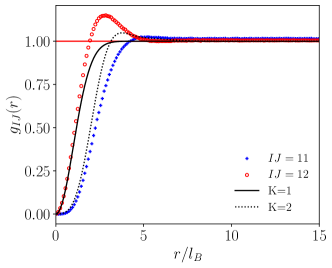
Figure 3: Pair correlation function for intra- and inter-species of $\begin{pmatrix}2&1\\ 1&2\end{pmatrix}$. The black lines are the pair correlation functions for single-species $K$-matrix $K=1$ (solid) and $K=2$ (dotted).

Next, we describe our computation of $V_{IJ}$. For single-species FQH state

$$\Psi(z_{i})=\hskip 1.0pt\mathrm{e}^{-\frac{\sum_{i}|z_{i}|^{2}}{4l_{b}^{2}}}\prod_{i<j}(z_{i}-z_{j})^{\bar{K}}$$ (153)

the electron density is given by $n_{e}=\frac{1}{2\pi l_{b}^{2}\bar{K}}$. Using the Metropolis Monte Carlo method, we can numerically estimate the pair distribution function $g(r)$. For this, we first place the electrons randomly, and follow the Metropolis-Hastings algorithm. We extend this to 2-species $K$-matrix. The general 2-species $K$-matrix is given as $K=\begin{pmatrix}a&c\\ c&b\end{pmatrix}$. For simplicity we maintain the same $l_{B}$ values, meaning that the $f_{I}$ may not be equal to each other. We maintain the condition that $\nu_{I}>0$ for all species. In this case, the filling fraction is $\nu=\frac{a+b-2c}{ab-c^{2}}$, giving $n_{e}=\frac{\nu}{2\pi l_{B}^{2}}$. For example, Fig. 3 denotes the pair correlation function for the $K$-matrix $\begin{pmatrix}2&1\\ 1&2\end{pmatrix}$, with the black lines being the pair correlation function for $K=1$ and $K=2$ respectively. We observe that there is higher inter-species electron pair density and lower intra-species electron pair density.

The reason for this deviation is that as intra-species electrons are more strongly repelled compared to inter-species electrons, compared to the default case the intra-species electrons can spread further from each other due to the lower repulsion with the inter-species electrons, and vice versa. Therefore, intra-species electrons contribute to lower Coulomb energy compared to the default one-species case as they are more further apart whereas the intra-species are more close to each other and contribute more Coulomb energy compared to the single-species case. Our numerical results are summarized in Table 3.

References

Onnes [1911]H. K. Onnes, The superconductivity of
mercury, Comm.
Phys. Lab. Univ. Leiden, Nos 119 120, 122 (1911).
Bardeen et al. [1957]J. Bardeen, L. N. Cooper, and J. R. Schrieffer, Theory of
superconductivity, Phys. Rev. 108, 1175 (1957).
Kalmeyer and Laughlin [1987]V. Kalmeyer and R. B. Laughlin, Equivalence of the
resonating-valence-bond and fractional quantum Hall states, Physical Review Letter 59, 2095 (1987).
Laughlin [1988]R. B. Laughlin, Physical Review Letter 60, 1057 (1988).
Wen et al. [1989]X.-G. Wen, F. Wilczek, and A. Zee, Chiral spin states and superconductivity, Phys. Rev. B 39, 11413 (1989).
Chen et al. [1989]Y. H. Chen, F. Wilczek,
E. Witten, and B. Halperin, J. Mod. Phys. B 3, 1001 (1989).
Wen and Zee [1991]X.-G. Wen and A. Zee, Topological structures, universality
classes, and statistics screening in the anyon superfluid, Phys. Rev. B 44, 274 (1991).
Tang and Wen [2013]E. Tang and X.-G. Wen, Superconductivity with intrinsic
topological order induced by pure coulomb interaction and time-reversal
symmetry breaking, Phys. Rev. B 88, 195117 (2013), arXiv:1306.1528 .
Wen [1989]X.-G. Wen, Vacuum degeneracy of chiral
spin states in compactified space, Phys. Rev. B 40, 7387 (1989).
Han et al. [2024]T. Han, Z. Lu,
Y. Yao, L. Shi, J. Yang, J. Seo, S. Ye, Z. Wu, M. Zhou,
H. Liu, G. Shi, Z. Hua, K. Watanabe, T. Taniguchi, P. Xiong, L. Fu, and L. Ju, Signatures of Chiral Superconductivity in Rhombohedral Graphene 10.48550/arXiv.2408.15233
(2024), arXiv:2408.15233 .
Cao et al. [2018]Y. Cao, V. Fatemi,
S. Fang, K. Watanabe, T. Taniguchi, E. Kaxiras, and P. Jarillo-Herrero, Unconventional superconductivity in magic-angle graphene
superlattices, Nature (London) 556, 43 (2018), arXiv:1803.02342 .
Zhang et al. [2023]Y. Zhang, R. Polski,
A. Thomson, É. Lantagne-Hurtubise,
C. Lewandowski, H. Zhou, K. Watanabe, T. Taniguchi, J. Alicea, and S. Nadj-Perge, Enhanced superconductivity in spin-orbit proximitized
bilayer graphene, Nature (London) 613, 268 (2023), arXiv:2205.05087 .
Holleis et al. [2023]L. Holleis, C. L. Patterson, Y. Zhang, Y. Vituri,
H. M. Yoo, H. Zhou, T. Taniguchi, K. Watanabe, E. Berg, S. Nadj-Perge, and A. F. Young, Nematicity and Orbital Depairing in Superconducting Bernal Bilayer Graphene
with Strong Spin Orbit Coupling 10.48550/arXiv.2303.00742
(2023), arXiv:2303.00742 .
Li et al. [2024]C. Li, F. Xu, B. Li, J. Li, G. Li, K. Watanabe, T. Taniguchi, B. Tong,
J. Shen, L. Lu, J. Jia, F. Wu, X. Liu, and T. Li, Tunable superconductivity in
electron- and hole-doped Bernal bilayer graphene, Nature (London) 631, 300
(2024), arXiv:2405.04479 .
Patterson et al. [2024]C. L. Patterson, O. I. Sheekey, T. B. Arp, L. F. W. Holleis, J. M. Koh, Y. Choi,
T. Xie, S. Xu, E. Redekop, G. Babikyan, H. Zhou, X. Cheng, T. Taniguchi, K. Watanabe, C. Jin, E. Lantagne-Hurtubise, J. Alicea, and A. F. Young, Superconductivity and spin canting in spin-orbit proximitized rhombohedral
trilayer graphene 10.48550/arXiv.2408.10190 (2024), arXiv:2408.10190 .
Choi et al. [2024]Y. Choi, Y. Choi,
M. Valentini, C. L. Patterson, L. F. W. Holleis, O. I. Sheekey, H. Stoyanov, X. Cheng, T. Taniguchi, K. Watanabe, and A. F. Young, Electric field control of superconductivity and quantized anomalous Hall
effects in rhombohedral tetralayer graphene 10.48550/arXiv.2408.12584
(2024), arXiv:2408.12584 [cond-mat.mes-hall] .
Dong et al. [2024]Z. Dong, É. Lantagne-Hurtubise, and J. Alicea, Superconductivity from spin-canting fluctuations in rhombohedral
graphene 10.48550/arXiv.2406.17036 (2024), arXiv:2406.17036 .
Chou et al. [2022]Y.-Z. Chou, F. Wu, and S. Das Sarma, Enhanced superconductivity through
virtual tunneling in Bernal bilayer graphene coupled to WSe2, Phys. Rev. B 106, L180502 (2022), arXiv:2206.09922 .
Jimeno-Pozo et al. [2023]A. Jimeno-Pozo, H. Sainz-Cruz, T. Cea,
P. A. Pantaleón, and F. Guinea, Superconductivity from electronic
interactions and spin-orbit enhancement in bilayer and trilayer graphene, Phys. Rev. B 107, L161106 (2023), arXiv:2210.02915 .
Wagner et al. [2023]G. Wagner, Y. H. Kwan, N. Bultinck,
S. H. Simon, and S. A. Parameswaran, Superconductivity from repulsive
interactions in Bernal-stacked bilayer graphene, arXiv e-prints 10.48550/arXiv.2302.00682
(2023), arXiv:2302.00682 .
Dong et al. [2023b]Z. Dong, A. V. Chubukov, and L. Levitov, Transformer
spin-triplet superconductivity at the onset of isospin order in bilayer
graphene, Phys. Rev. B 107, 174512 (2023b), arXiv:2205.13353 .
Chau et al. [2024]C. W. Chau, S. A. Chen, and K. T. Law, Origin of Superconductivity in
Rhombohedral Trilayer Graphene: Quasiparticle Pairing within the Inter-Valley
Coherent Phase 10.48550/arXiv.2404.19237 (2024), arXiv:2404.19237 .
Chou et al. [2024]Y.-Z. Chou, J. Zhu, and S. D. Sarma, Intravalley spin-polarized superconductivity in
rhombohedral tetralayer graphene (2024), arXiv:2409.06701 .
Geier et al. [2024]M. Geier, M. Davydova, and L. Fu, Chiral and topological superconductivity in isospin
polarized multilayer graphene (2024), arXiv:2409.13829 .
Zhang et al. [1989]S. C. Zhang, T. H. Hansson, and S. Kivelson, Effective-field-theory model for the
fractional quantum Hall effect, Physical Review Letter 62, 82 (1989).
Wen and Zee [1990]X.-G. Wen and A. Zee, Compressibility and superfluidity in
the fractional-statistics liquid, Phys. Rev. B 41, 240 (1990).
Wen and Zee [1992]X.-G. Wen and A. Zee, Classification of Abelian quantum
Hall states and matrix formulation of topological fluids, Phys. Rev. B 46, 2290 (1992).
Han et al. [2023]T. Han, Z. Lu,
G. Scuri, J. Sung, J. Wang, T. Han, K. Watanabe, T. Taniguchi, H. Park, and L. Ju, Correlated Insulator and Chern Insulators in Pentalayer Rhombohedral
Stacked Graphene 10.48550/arXiv.2305.03151 (2023), arXiv:2305.03151 .
Tanatar and Ceperley [1989]B. Tanatar and D. M. Ceperley, Ground state of the
two-dimensional electron gas, Phys. Rev. B 39, 5005 (1989).
Lu et al. [2023]Z. Lu, T. Han,
Y. Yao, A. P. Reddy, J. Yang, J. Seo, K. Watanabe, T. Taniguchi, L. Fu, and L. Ju, Fractional Quantum Anomalous Hall Effect in a Graphene Moire
Superlattice 10.48550/arXiv.2309.17436 (2023), arXiv:2309.17436 .
Cai et al. [2023]J. Cai, E. Anderson,
C. Wang, X. Zhang, X. Liu, W. Holtzmann, Y. Zhang, F. Fan, T. Taniguchi, K. Watanabe, Y. Ran, T. Cao, L. Fu, D. Xiao, W. Yao, and X. Xu, Signatures of Fractional Quantum Anomalous Hall
States in Twisted MoTe2 Bilayer 10.48550/arXiv.2304.08470
(2023), arXiv:2304.08470 .
Park et al. [2023]H. Park, J. Cai,
E. Anderson, Y. Zhang, J. Zhu, X. Liu, C. Wang, W. Holtzmann, C. Hu, Z. Liu, T. Taniguchi,
K. Watanabe, J.-h. Chu, T. Cao, L. Fu, W. Yao, C.-Z. Chang,
D. Cobden, D. Xiao, and X. Xu, Observation of Fractionally Quantized Anomalous Hall Effect 10.48550/arXiv.2308.02657 (2023), arXiv:2308.02657 .
Xu et al. [2023]F. Xu, Z. Sun,
T. Jia, C. Liu, C. Xu, C. Li, Y. Gu, K. Watanabe,
T. Taniguchi, B. Tong, J. Jia, Z. Shi, S. Jiang, Y. Zhang, X. Liu, and T. Li, Observation of integer and fractional quantum anomalous Hall effects in
twisted bilayer MoTe2 10.48550/arXiv.2308.06177 (2023), arXiv:2308.06177 .
Shi and Senthil [2024]Z. D. Shi and T. Senthil, Doping a fractional quantum anomalous hall
insulator (2024), arXiv:2409.20567 .
Lan et al. [2016]T. Lan, L. Kong, and X.-G. Wen, Theory of (2+1)-dimensional fermionic topological
orders and fermionic/bosonic topological orders with symmetries, Phys. Rev. B 94, 155113 (2016), arXiv:1507.04673 .