Magnetohydrodynamic simulations of A-type stars:
Long-term evolution of core dynamo cycles

Abstract

Context. Early-type stars have convective cores due to a steep temperature gradient produced by the CNO cycle. These cores can host dynamos, and the generated magnetic fields can be relevant to explain the magnetism observed in Ap/Bp stars.

Aims. Our main objective is to characterise the convective core dynamos and differential rotation, and to do the first quantitative analysis of the relation between magnetic activity cycle and rotation period.

Methods. We use numerical 3D star-in-a-box simulations of a $2.2\leavevmode\nobreak\ M_{\odot}$ A-type star with a convective core of roughly 20% of the stellar radius surrounded by a radiative envelope. Rotation rates from 8 to 20 days are explored. We use two models of the entire star, and an additional zoom set, where 50% of the radius is retained.

Results. The simulations produce hemispheric core dynamos with cycles and typical magnetic field strengths around $60$ kG. However, only a very small fraction of the magnetic energy is able to reach the surface. The cores have solar-like differential rotation, and a substantial part of the radiative envelope has quasi-rigid rotation. In the most rapidly rotating cases the magnetic energy in the core is roughly 40% of the kinetic energy. Finally, we find that the magnetic cycle period $P_{\mathrm{cyc}}$ increases with decreasing the rotation period $P_{\mathrm{rot}}$ which is also observed in many simulations of solar-type stars.

Conclusions. Our simulations indicate that a strong hemispherical core dynamo arises routinely, but that it is not enough the explain the surface magnetism of Ap/Bp stars. Nevertheless, as the core dynamo produces dynamically relevant magnetic fields it should not be neglected when other mechanisms are explored.

1 Introduction

Magnetic fields can be found in a wide variety of stars, and there is a general consensus that most of them are amplified and maintained via self-excited dynamos. In this context, these processes typically require rotation and fluid motions, and therefore are most likely to occur inside convection zones (see Brandenburg & Subramanian 2005; Brun & Browning 2017). The most obvious example is the Sun, which has a cyclic large-scale magnetic field driven by a self-excited dynamo operating in its convective envelope (see e.g. Charbonneau 2020). Like the Sun, other late-type stars (M, K, F) have convective envelopes, and the observed magnetic fields in these stars have also very likely a convective origin. Numerical simulations targeting a wide variety of rotating fully or partially convective stars yield dynamos of various sorts (see, e.g. Käpylä et al., 2023, and references therein).

Early-type main-sequence stars have masses $M>1.5\leavevmode\nobreak\ M_{\odot}$ and effective temperatures $T_{\rm eff}\gtrsim 10^{4}$ K. Roughly $10\%$ of early-type stars are magnetic (see e.g. Kochukhov & Bagnulo, 2006; Landstreet et al., 2007, 2008; Grunhut et al., 2017; Shultz et al., 2019). According to our understanding of stellar evolution, these stars have radiative, and therefore stably stratified, envelopes. This might explain why a dynamo cannot usually operate near the surfaces of these stars, since vigorous fluid motions are absent. However, some stars in the range $1.5\leavevmode\nobreak\ M_{\odot}$ to $6\leavevmode\nobreak\ M_{\odot}$ host observable large-scale magnetic fields. The best example is the subgroup of chemically peculiar main-sequence stars, classified as Ap/Bp. These stars host magnetic fields with mean field strengths ranging from $200\leavevmode\nobreak\ \mathrm{G}$ to $30\leavevmode\nobreak\ \mathrm{kG}$ (Aurière et al., 2007), the strongest field being $34\leavevmode\nobreak\ \mathrm{kG}$ in HD 215441 (Babcock, 1960). Roughly $10\%$ of A-type stars belong to the sub-classification Ap and have detectable strong magnetic fields (Moss, 2001). The non-magnetised population (“normal” A-type stars) usually have very weak fields below the detection limit. Nevertheless, weak magnetic fields have been detected in the normal population, for example in Sirius and Vega. In the case of Vega, Zeeman polarimetry gives a magnetic field strength of $0.6\pm 0.3$ G (Lignières et al., 2009; Petit et al., 2010, 2022), and $0.2\pm 0.1$ G for Sirius (Petit et al., 2011). Normal A stars are typically rapid rotators (Royer et al., 2007), whereas Ap stars are slower rotators than their non-magnetic counterparts (Abt & Morrell, 1995). Indeed, Mathys (2008) have shown that non-magnetic A stars have rotation periods ranging from a few hours to a day, while most Ap stars have periods between one and ten days. This could be an indication of magnetic braking, although there is no clear correlation between rotation and magnetic fields (Kochukhov & Bagnulo, 2006).

The origin of the large-scale magnetic fields in Ap/Bp stars remains uncertain, although several theories have been proposed. The fossil field theory suggests that these magnetic fields originate from the protostellar phase of the star. The Ohmic diffusion time in radiative zones is very long (e.g. $10^{10}$ years in the context of the Sun, Cowling 1945), and therefore, a magnetic field in equilibrium in a radiative zone could survive the whole main-sequence life of the star. Stable magnetic configurations in fully radiative A-type stars have been reported in numerical simulations (Braithwaite & Spruit, 2004; Braithwaite & Nordlund, 2006; Braithwaite, 2008; Becerra et al., 2022). In principle, the fossil magnetic field has to survive the convective protostellar phase as the star descends the Hayashi track (Hayashi et al., 1962; Siess et al., 2000). This appears to be very unlikely assuming a fully convective evolution, but a transition to a radiative phase could counterbalance this problem and preserve a significant part of the initial magnetic flux (Schleicher et al., 2023). Such protostellar models were proposed e.g. by Palla & Stahler (1992, 1993).

Alternatively, it has been proposed that radiative envelopes can host dynamos, as a result of the interaction between a magnetic instability (e.g. Tayler, 1973) and differential rotation. This is the Tayler-Spruit dynamo scenario (Spruit, 2002). Recently, Petitdemange et al. (2023, 2024) performed global simulations of a magnetised stably stratified fluid with differential rotation in a spherical shell, reporting the first numerical demonstration of the Tayler-Spruit dynamo.

Another alternative is a strong core dynamo. Early-type stars have convective cores due to the temperature sensitivity of the dominant nuclear reaction (CNO cycle) such that energy production is highly concentrated in the centre of the star, leading to a steep temperature gradient that drives convection. It was long suspected that the convective cores in A stars host dynamos (Krause & Oetken, 1976). Simulations by Browning et al. (2004) showed that such convective cores have differential rotation that is beneficial for dynamo action. This was reported by Brun et al. (2005), who performed numerical simulations of the inner $30\%$ by radius (half of which was convective) of a $2\leavevmode\nobreak\ M_{\odot}$ A-type star, obtaining magnetic fields with typical strengths around equipartition with kinetic energy. Interestingly, the inclusion of a fossil field in the radiative envelope might affect the nature of the core dynamo (see, e.g. Boyer & Levy, 1984, in the context of the Sun). Featherstone et al. (2009) performed simulations of the core dynamo from a $2\leavevmode\nobreak\ M_{\odot}$ A-type star, reporting an equipartition magnetic field. However, the inclusion of a twisted toroidal fossil field can lead to a superequipartition state in the core, where the magnetic energy is roughly 10 times stronger than the kinetic energy. In B-type stars, dynamos have been found as well. Simulations by Augustson et al. (2016) of the core of a $10\leavevmode\nobreak\ M_{\odot}$ B-type star, showed vigorous dynamo action, and generated superequipartition magnetic fields with peak values exceeding a megagauss in the rapid rotators. However, although these studies show that a convective core can lead to strong dynamo action, the nature of these dynamos has not been explored in detail. For example, no cyclic solutions or a relation between the magnetic cycle period to rotation period of the core dynamo have been reported.

A natural question is whether the magnetic fields generated in the core can reach the surface of the star. This could happen under the action of buoyancy. Stellar structure models predict convection zones close to the surface of early-type stars (Richard et al., 2001; Cantiello et al., 2009) due to bumps in the stellar opacities from iron (Iglesias et al., 1992), hydrogen and helium ionisation. These layers can host dynamos and the resulting magnetic field, could easily rise to the surface due to magnetic buoyancy, creating surface magnetic fields of order a few Gauss (Cantiello & Braithwaite, 2019). In principle, the same could happen in the context of a core dynamo. However, the timescale of this process has been estimated to be longer than the main-sequence lifetime of these stars (Schuessler & Paehler, 1978; Parker, 1979; Moss, 1989), unless the magnetic structures are very small. This was reported by MacGregor & Cassinelli (2003), who modelled a buoyant magnetic flux ring in the radiative interior of an early-type star (with $M<10\leavevmode\nobreak\ M_{\odot}$), and found transport timescales that were shorter than the main-sequence lifetime of the star. Nonetheless, MacDonald & Mullan (2004) re-examined the conclusions of MacGregor & Cassinelli (2003) with more realistic models including differential rotation and realistic strong compositional gradients in the radiative layers. This slows down the buoyancy process considerably, and magnetic fields higher than the equipartition values are required to make this process feasible. One mechanism that could counter this situation is convective overshooting. This could allow mixing in the stably stratified zone above the convective core, reducing the compositional gradient. Also, the field that penetrates the radiative envelope might be strengthened by the shearing produced by the differential rotation, making it strong enough to reach the surface due to buoyancy.

Core dynamo simulations often include the convective core and only a part of the radiative envelope of the star (e.g. Brun et al., 2005; Augustson et al., 2016). In the current study, we perform simulations of a main-sequence A-type star using the star-in-a-box model. This setup allows us to explore dynamo action generated by convection in the core of the star (including $r=0$), and study the resulting magnetic field not only in the core but also on the stellar surface, modelling the entire star for the first time in 3D numerical simulations. Another point of interest is to study magnetic cycles and their relation to the rotation period. The relation between these quantities has been studied before in simulations of other types of stars (see e.g. Warnecke, 2018; Strugarek et al., 2018, for solar-like stars), but such relation has not been presented before in the context of A-type stars. The models as well as the methods are described in Section 2. The analysis and results of the simulations are provided in Section 3. Discussion and conclusions of this study are presented in Section 4.

2 Numerical models and methods

2.1 Full star setup

The model used here is based on the star-in-a-box setup presented by Käpylä (2021), which is based on the setup by Dobler et al. (2006). The computational domain corresponds to a box of side $l=2.2R$, where $R$ is the stellar radius and all coordinates $(x,y,z)$ range from $-l/2$ to $l/2$. The following non-ideal fully compressible MHD equation set is solved:

$$\frac{\partial\bm{A}}{\partial t} =\bm{U}\times\bm{B}-\eta\mu_{0}\bm{J},$$ (1)

$$\frac{D\ln\rho}{Dt} =-\bm{\nabla}\bm{\cdot}\bm{U},$$ (2)

$$\frac{D\bm{U}}{Dt} =-\bm{\nabla}\Phi-\frac{1}{\rho}\left(\bm{\nabla}p-\bm{\nabla}\bm{\cdot}2\nu\rho\bm{\mathsf{S}}+\bm{J}\times\bm{B}\right)-2\bm{\Omega}\times\bm{U}+\bm{f}_{d},$$ (3)

$$T\frac{Ds}{Dt} =-\frac{1}{\rho}\left[\bm{\nabla}\bm{\cdot}(\bm{F}_{\text{rad}}+\bm{F}_{\text{SGS}})+\mathcal{H}-\mathcal{C}+\mu_{0}\eta\bm{J}^{2}\right]+2\nu\bm{\mathsf{S}}^{2},$$ (4)

where $\bm{A}$ is the magnetic vector potential, $\bm{U}$ is the flow velocity, $\bm{B}=\bm{\nabla}\times\bm{A}$ is the magnetic field, $\eta$ is the magnetic diffusivity, $\mu_{0}$ is the magnetic permeability of vacuum, $\bm{J}=\bm{\nabla}\times\bm{B}/\mu_{0}$ is the current density given by Ampère’s law, $D/Dt=\partial/\partial t+\bm{U}\bm{\cdot}\bm{\nabla}$ is the advective (or material) derivative, $\rho$ is the mass density, $p$ is the pressure, $\Phi$ is the fixed gravitational potential, given by the Padé approximation obtained from 1D stellar structure model:

$$\Phi(r^{\prime})=-\frac{GM}{R}\frac{a_{0}+a_{2}r^{\prime 2}+a_{3}r^{\prime 3}}{1+b_{2}r^{\prime 2}+b_{3}r^{\prime 3}+a_{3}r^{\prime 4}},$$ (5)

where $r^{\prime}=r/R$ is the fractional radius, $G$ is the gravitational constant, $M$ is the mass of the star. For an A0-type star the coefficients are given by $a_{0}=4.3641$, $a_{2}=-1.5612$, $a_{3}=0.4841$, $b_{2}=4.0678$, and $b_{3}=1.2548$. $\nu$ is the kinematic viscosity, $\bm{\mathsf{S}}$ is the traceless rate-of-strain tensor, given by

$$\mathsf{S}_{ij}=\frac{1}{2}(\partial_{j}U_{i}+\partial_{i}U_{j})-\frac{1}{3}\delta_{ij}\bm{\nabla}\bm{\cdot}\bm{U},$$ (6)

where $\delta_{ij}$ is the Kronecker delta. $\bm{\Omega}=(0,0,\Omega_{0})$ is the rotation vector and $\bm{f}_{\mathrm{d}}$ describes damping of flows exterior to the star, given by

$$\bm{f}_{d}=-\frac{\bm{U}}{\tau_{\text{damp}}}f_{e}(r),$$ (7)

where $\tau_{\text{damp}}=0.2\tau_{\mathrm{ff}}\approx 1.5\leavevmode\nobreak\ \mathrm{days}$ is the damping timescale and $\tau_{\mathrm{ff}}=\sqrt{R^{3}/GM}$ is the freefall time. The function $f_{e}(r)$ is defined as

$$f_{e}(r)=\frac{1}{2}\left(1+\tanh\frac{r-r_{\text{damp}}}{w_{\text{damp}}}\right),$$ (8)

where $r_{\text{damp}}=1.03R$ is the damping radius and $w_{\text{damp}}=0.02R$ is its width. $T$ is the temperature, $s$ is the specific entropy, $\bm{F}_{\mathrm{rad}}$ is the radiative flux and $\bm{F}_{\mathrm{SGS}}$ is the subgrid-scale (SGS) entropy flux. Radiation inside the star is approximated as a diffusion process. Therefore, the radiative flux is given by

$$\bm{F}_{\mathrm{rad}}=-K\bm{\nabla}T,$$ (9)

where $K$ is the radiative heat conductivity, a quantity that is assumed to be constant. In addition, it is convenient to introduce a SGS entropy diffusion that does not contribute to the net energy transport, but damps fluctuations near the grid scale. This is given by the SGS entropy flux

$$\bm{F}_{\mathrm{SGS}}=-\chi_{\mathrm{SGS}}\rho\bm{\nabla}s^{\prime},$$ (10)

where $\chi_{\mathrm{SGS}}$ is the SGS diffusion coefficient, and

$$s^{\prime}=s-\langle s\rangle_{t}$$ (11)

is the fluctuating entropy, where $\langle s\rangle_{t}(\bm{x})$ is a running temporal mean of the specific entropy. $\mathcal{H}$ and $\mathcal{C}$ describe additional heating and cooling, respectively, and we adopted similar expressions as in Dobler et al. (2006) and Käpylä (2021), where

$$\mathcal{H}(r)=\frac{L_{\text{sim}}}{(2\pi w_{L}^{2})^{3/2}}\exp\left(-\frac{r^{2}}{2w_{L}^{2}}\right),$$ (12)

is a normalised Gaussian profile that parameterises the nuclear energy production inside the core of the star, where $L_{\text{sim}}$ is the luminosity in the simulation, and $w_{L}=0.1R$ is the width of the Gaussian. Furthermore, $\mathcal{C}(\bm{x})$ models the radiative losses above the stellar surface, and it is given by

$$\mathcal{C}(\bm{x})=\rho c_{\text{P}}\frac{T(\bm{x})-T_{\text{surf}}}{\tau_{\text{cool}}}f_{e}(r),$$ (13)

where $c_{\rm P}$ is the heat capacity at constant pressure, $T_{\text{surf}}=T(R)$ is the temperature at the surface of the star, $\tau_{\text{cool}}=\tau_{\text{damp}}$ is a cooling timescale, and $f_{e}(r)$ is given by Eq. (8), with the same parameters, $r_{\text{cool}}=r_{\text{damp}}$ and $w_{\text{cool}}=w_{\text{damp}}$. The ideal gas equation of state $p=\mathcal{R}\rho T$ is assumed, where $\mathcal{R}=c_{\rm P}-c_{\rm V}$ is the ideal gas constant, and $c_{\rm V}$ is the heat capacity at constant volume.

To avoid diffusive spreading of magnetic fields and flows from the core to the envelope we follow Käpylä (2022), and use radial profiles for the diffusivities $\nu$ and $\eta$, where the radiative layers have values $10^{2}$ times smaller than the core. The magnetic diffusivity has to be already rather low in the core to excite a dynamo; see Sect. 3. Therefore the diffusivities in the radiative envelope are even lower making it hard to resolve the flows and magnetic fields there. To cope with this issue, we add artificial sixth-order hyperdiffusivity terms in the dynamical equations. The hyperdiffusive terms smooth small scale oscillation to avoid numerical instabilities near grid scale (see e.g. Brandenburg & Sarson, 2002; Johansen & Klahr, 2005). Here we use the resolution-independent mesh hyper-Reynolds number method described in the Appendix A of Lyra et al. (2017) for $\nu$ and $\eta$, in all the sets of simulations. Furthermore, the advective terms of Eqs. (1) to (4) are written in terms of fifth-order upwinding derivatives with a sixth-order hyperdiffusive correction with a flow dependent diffusion coefficient; see Appendix B of Dobler et al. (2006).

2.2 Zoom setup

Modelling the whole star allows us to study the convective core all the way to the surface of the star. However, this also reduces the number of grid points available to resolve convection inside the core. To test the robustness of the results and to increase the spatial resolution in the core, we run a few simulations using a zoom model, which is otherwise the same as the full star model, but the box has a side of $l=1.1R$. Therefore, we exclude the surface of the star and focus exclusively in the convective core with higher resolution.

The flow damping radius was changed to $r_{\mathrm{damp}}=0.45R$ with $\tau_{\mathrm{damp}}=0.02\tau_{\mathrm{ff}}\approx 0.15$ days, and $w_{\mathrm{damp}}=0.01R$, and the cooling now starts at $r_{\mathrm{cool}}=0.52R$, with $w_{\mathrm{cool}}=0.02R$ and $\tau_{\mathrm{cool}}=0.2\tau_{\mathrm{ff}}\approx 1.5\leavevmode\nobreak\ \mathrm{days}$. These choices were made more out of numerical convenience rather than physical arguments. However, as will be shown in Sect. 3 the main results remain unaffected.

2.3 Physical units, initial and boundary conditions

The stellar parameters are extracted from a $2.2\leavevmode\nobreak\ M_{\odot}$ main-sequence one dimensional stellar model. This model was obtained using the MESA code (see Paxton et al., 2019, and the references therein). The radius, mass density and temperature of the stellar centre, and luminosity averaged from $t=2.5\cdot 10^{6}$ years to $t=4.5\cdot 10^{8}$ years are given by $R_{*}=2.1\leavevmode\nobreak\ R_{\odot}$, $\rho_{0}=5.5\cdot 10^{4}\leavevmode\nobreak\ \mathrm{kg}\,\mathrm{m^{-3}}$, $T_{0}=2.3\cdot 10^{7}\leavevmode\nobreak\ \mathrm{K}$ and $L_{*}=23.5\leavevmode\nobreak\ L_{\odot}$, where $L_{\odot}=3.83\cdot 10^{26}$ W is the solar luminosity, respectively. Furthermore, the surface gravity is:

$$g_{*}=\frac{GM_{*}}{R_{*}^{2}}\approx\frac{2.2}{2.1^{2}}\frac{GM_{\odot}}{R_{\odot}^{2}}\approx 0.5g_{\odot}=137\leavevmode\nobreak\ \frac{\mathrm{m}}{\mathrm{s^{2}}},$$ (14)

where $g_{\odot}=274\leavevmode\nobreak\ \mathrm{m\,s^{-2}}$. Using realistic parameters in fully compressible simulations of stars is infeasible due to the huge gap between the acoustic (dynamic) and Kelvin-Helmholtz (thermal) timescales. A solution to this problem was originally pointed out by Chan & Sofia (1986), and it consists of exaggerating the luminosity in numerical simulations. Here we follow the notation of Dobler et al. (2006) and define a dimensionless luminosity

$$\mathcal{L}=\frac{L}{\sqrt{G^{3}M^{5}/R^{5}}},$$ (15)

with which we define the luminosity ratio between the simulation and the target star:

$$L_{\mathrm{ratio}}=\frac{\mathcal{L}_{\mathrm{sim}}}{\mathcal{L}_{\mathrm{star}}}.$$ (16)

Now, the gap between acoustic and Kelvin-Helmholtz timescales is reduced by a cumulative factor of $L_{\mathrm{ratio}}^{4/3}$ (see Käpylä, 2021, for a detailed discussion).

The units of length and time are given by the radius of the star $[x]=R$ and the free-fall time $[t]=\tau_{\mathrm{ff}}$ respectively. Furthermore, the unit of magnetic field is obtained from the equipartition field strength as $[B]=\sqrt{\mu_{0}\rho_{0}}[x]/[t]$, and the unit of entropy is $[s]=c_{\rm P}$. The conversion factors between simulation and physical units are (for example, $x=x_{\mathrm{fac}}x_{\mathrm{sim}}$, see Käpylä et al., 2020)

$$x_{\mathrm{fac}}=\frac{R_{*}}{R_{\mathrm{sim}}},\hskip 14.22636ptt_{\mathrm{fac}}=\frac{\Omega_{\mathrm{sim}}}{\Omega_{*}},\hskip 14.22636ptU_{\mathrm{fac}}=\frac{R_{*}\Omega_{*}}{R_{\mathrm{sim}}\Omega_{\mathrm{sim}}},$$ (17)

$$\rho_{\mathrm{fac}}=\frac{\rho_{0}}{\rho_{\mathrm{0,sim}}},\hskip 14.22636ptB_{\mathrm{fac}}=\left[\frac{\mu_{0}\rho_{0}(\Omega_{*}R_{*})^{2}}{\mu_{\mathrm{0,sim}}\rho_{\mathrm{0,sim}}(\Omega_{\mathrm{sim}}R_{\mathrm{sim}})^{2}}\right]^{1/2},$$ (18)

where the subscript “sim” represents the quantity in simulation units. Furthermore, since the convective velocity scales with luminosity as $u_{\mathrm{conv}}\propto L^{1/3}$ (Jones et al., 2017; Käpylä et al., 2020; Baraffe et al., 2023; Käpylä, 2024), the rotation rate needs to be enhanced by the same factor ($L_{\mathrm{ratio}}^{1/3}$) to have a consistent rotational influence on the flow. Following Appendix A of Käpylä et al. (2020), we obtain

$$\Omega_{\mathrm{sim}}=L_{\mathrm{ratio}}^{1/3}\left(\frac{g_{\mathrm{sim}}}{g_{*}}\frac{R_{*}}{R_{\mathrm{sim}}}\right)^{1/2}\Omega_{*}.$$ (19)

The convective core is assumed to encompass $20\%$ of the stellar radius. To set such configuration we assume a piecewise polytropic initial state. A polytrope is defined by

$$p(\rho)=K_{0}\rho^{\gamma},$$ (20)

where $K_{0}$ is a constant, and

$$\gamma=\frac{d\ln p}{d\ln\rho}=1+\frac{1}{n}$$ (21)

is the adiabatic index written in terms of the polytropic index $n$. We choose $n=n_{\rm ad}=1.5$ in the convectively unstable layer ($r<0.2R$), and $n=n_{\rm rad}=3.25$ in the stable layer ($r>0.2R$) with a smooth transition between them. Here $n_{\rm ad}$ corresponds to a marginally stable stratification whereas $n_{\rm rad}$ arises in a hydrostatic solution of a radiative atmosphere with Kramers opacity law (e.g. Barekat & Brandenburg, 2014).

The boundary conditions are impenetrable and stress-free conditions for flow and the magnetic field is assumed to be perpendicular to the boundary. We further assume a vanishing second derivative for $\ln\rho$, and vanishing temperature gradient across the exterior boundaries of the box. For the initial conditions of the flow and magnetic field, we considered low amplitude Gaussian noise with initial amplitudes of $2\cdot 10^{-3}$ m/s and $1$ G respectively.

The simulations were run with the Pencil Code (Brandenburg & Dobler, 2002; Pencil Code Collaboration et al., 2021), which is a highly modular high-order finite-difference code for solving partial differential equations.

2.4 Dimensionless parameters

To characterise our simulations, the following dimensionless numbers are computed. The effect of rotation relative to viscous forces is measured by the Taylor number

$$\mathrm{Ta}=\frac{4\Omega_{0}^{2}\Delta r^{4}}{\nu^{2}},$$ (22)

where $\Delta r=0.2R$ is the depth of the convective zone. The magnetic and SGS Prandtl numbers are

$$\mathrm{Pr}_{\mathrm{M}}=\frac{\nu}{\eta},\hskip 14.22636pt\mathrm{Pr}_{\mathrm{SGS}}=\frac{\nu}{\chi_{\mathrm{SGS}}}.$$

The influence of rotation on the flow is measured by the Coriolis number

$$\mathrm{Co}=\frac{2\Omega_{0}}{u_{\mathrm{rms}}k_{R}},$$ (23)

where $u_{\mathrm{rms}}$ is the root-mean-square (rms) velocity averaged over the convective zone ($r<\Delta r$) and $k_{R}=2\pi/\Delta r$ is the scale of the largest convective eddies. The fluid and magnetic Reynolds numbers are defined as

$$\mathrm{Re}=\frac{u_{\mathrm{rms}}}{\nu k_{R}},\hskip 14.22636pt\mathrm{Re_{M}}=\frac{u_{\mathrm{rms}}}{\eta k_{R}},$$ (24)

and the SGS Péclet number is

$$\mathrm{Pe}=\frac{u_{\mathrm{rms}}}{\chi_{\mathrm{SGS}}k_{R}}.$$ (25)

Furthermore, the Brunt-Väisälä (or buoyancy) frequency and the Richardson number related to rotation in the radiative zone are defined as

$$N=\sqrt{\frac{g}{c_{\mathrm{P}}}\frac{ds}{dr}},\hskip 14.22636pt\mathrm{Ri}_{\Omega}=\frac{N^{2}}{\Omega_{0}^{2}},$$ (26)

respectively. If $N^{2}>0$, then the layer will be stable against buoyancy fluctuations.

3 Results

Table 1: Summary of the simulations.

Run	$P_{\mathrm{rot}}$ [days]	$u_{\mathrm{rms}}$ [m/s]	$B_{\mathrm{rms}}$ [kG]	Co	Ta[$10^{8}$]	Pe	Re	$\mathrm{Re}_{\mathrm{M}}$	$\mathrm{Ri}_{\Omega}[10^{-2}]$	$P_{\mathrm{cyc}}$ [years]
MHDr1	20	99	no dynamo	5.0	1.10	11	52	36	16.0	-
MHDr2	15	51	60	10.1	1.95	7	35	24	9.2	$1.81\pm 0.10$
MHDr2*	15	52	57	9.9	1.95	7	35	25	9.2	$2.14\pm 0.13$
MHDr3	10	39	65	19.2	4.38	5	27	19	4.1	$2.50\pm 0.11$
MHDr3*	10	39	62	18.8	4.38	5	28	19	3.9	$2.62\pm 0.14$
MHDr4	8	35	60	26.9	6.84	5	24	17	2.6	$3.14\pm 0.05$
MHDr4*	8	35	57	26.2	6.84	5	25	17	2.5	$3.37\pm 0.08$
zMHDr1	20	95	not saturated	4.9	1.10	11	53	37	16.8	-
zMHDr2	15	55	49	9.6	1.95	7	36	25	9.6	$1.95\pm 0.03$
zMHDr3	10	39	53	18.9	4.38	5	28	19	4.3	$2.60\pm 0.03$
zMHDr4	8	36	46	26.9	6.84	5	24	17	2.7	$2.50\pm 0.02$

We present three sets of simulations exploring rotation periods from 8 to 20 days. All simulations have $\nu=5.45\cdot 10^{7}\leavevmode\nobreak\ \mathrm{m^{2}/s}$, $\eta=7.78\cdot 10^{7}\leavevmode\nobreak\ \mathrm{m^{2}/s}$, and $\chi_{\mathrm{SGS}}=2.61\cdot 10^{8}\leavevmode\nobreak\ \mathrm{m^{2}/s}$ in the core, and therefore $\mathrm{Pr}_{\mathrm{M}}=0.7$ and $\mathrm{Pr}_{\mathrm{SGS}}\approx 0.21$. In the first set of simulations (group MHD), $\nu$ and $\eta$ have radial jumps around $0.35R$, with a smooth transition over a width of $0.06R$. Above the jump, diffusivities are $10^{2}$ times smaller. In the second set (group MHD*) the jump is at $0.3R$ and its width is $0.03R$. Simulations in this group start from already saturated snapshots of the respective simulation with the same rotation rate in the MHD group. The third set corresponds to the zoom setup (group zMHD) described in Section 2.2. The radial profiles are the same as those in group MHD. The runs, as well as the diagnostic quantities are listed in Table 2. All simulations were run on a grid of $200^{3}$ uniformly distributed grid points.

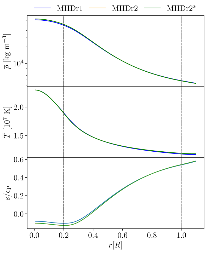
Figure 1: Top panel: Density profiles as functions of radius from MHDr1, MHDr2, and MHDr2*. Middle panel: Temperature profiles for the same runs. Bottom panel: Specific entropy profiles from the same runs. The black dashed line indicates the surface of the convective core ($r=0.2R$) and the grey dashed line the stellar surface ($r=R$). The quantities are time-averaged over the thermally relaxed phase.

Figure 1 shows the radial profiles of density, temperature, and specific entropy from representative runs, where the overlines denote horizontal ($\phi\theta$) averaging. The density stratification between the centre and the surface of the star ($r=R$) is $\overline{\rho}_{\mathrm{centre}}/\overline{\rho}_{\mathrm{surface}}\approx 13$ in the full star runs. Furthermore, the stratification between the centre and the surface of the convective core ($r=0.2R$) is $\overline{\rho}_{\mathrm{centre}}/\overline{\rho}_{\mathrm{surfcore}}\approx 1.27$, which is close to that from the MESA model $\overline{\rho}_{\mathrm{centre}}/\overline{\rho}_{\mathrm{surfcore}}\approx 1.5$. The same ratios for the temperature are $\overline{T}_{\mathrm{centre}}/\overline{T}_{\mathrm{surface}}\approx 2$ and $\overline{T}_{\mathrm{centre}}/\overline{T}_{\mathrm{surfcore}}\approx 1.23$. From the lower panel of Figure 1, we can infer a negative entropy gradient in the convective core and a positive gradient at the rest of the star, which is the expected configuration for a A-type main-sequence star. The surface cooling becomes effective above $r_{\rm cool}$ and relaxes the regions exterior to the star toward a constant temperature $T_{\rm surf}$. Therefore the density drops nearly exponentially above $r=r_{\rm cool}$. Radiation transports all of the energy in the stellar envelope all the way to the surface; see Sect. 3.3.2. This means that the photosphere at the stellar surface is modelled in a very simplistic way where the energy transport mechanism switches from radiative diffusion to the cooling flux which mimics radiative losses in the optically thin exterior. This approach avoids detailed physics leading to, for example, thin convection zones near the surface. Since the focus in the current study is in the core dynamo, this simplification is justified.

Finally, the stratification in the cores of the simulations in group zMHD is similar to those in the full star models, and the density and temperature ratios between the centre of the star and the outer edge of the radiative zone ($r=0.55R$) are $\overline{\rho}_{\mathrm{centre}}/\overline{\rho}_{\mathrm{edge}}\approx 4.15$, and $\overline{T}_{\mathrm{centre}}/\overline{T}_{\mathrm{edge}}\approx 1.6$.

3.1 Dynamo solutions

All of our runs, except for MHDr1, host a dynamo. In the corresponding Run zMHDr1 the magnetic field grows but the dynamo is very close to marginal, and it is impractical to run it to saturation.

3.1.1 Core dynamos

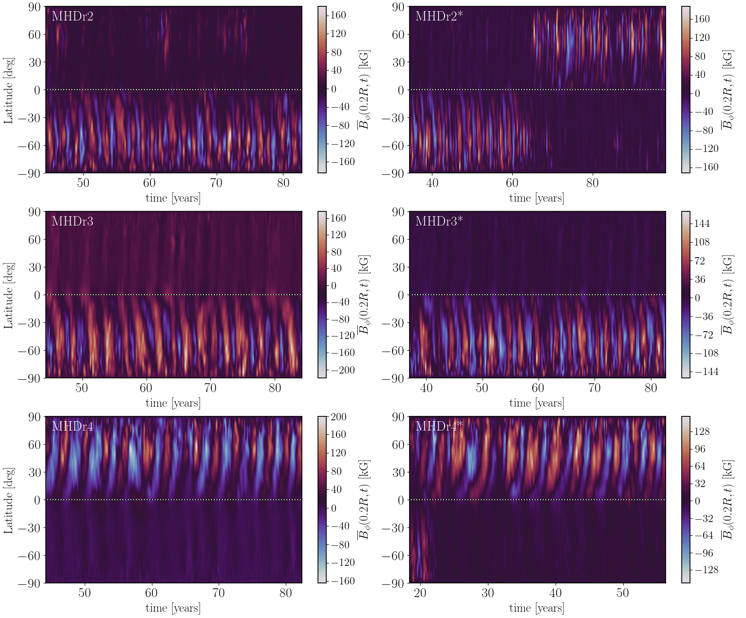
Figure 2: Time-latitude diagrams of the azimuthally averaged toroidal magnetic field $\overline{B}_{\phi}(r=0.2R,\theta,t)$ of the full star models. The run is indicated in the upper left corner of each panel.

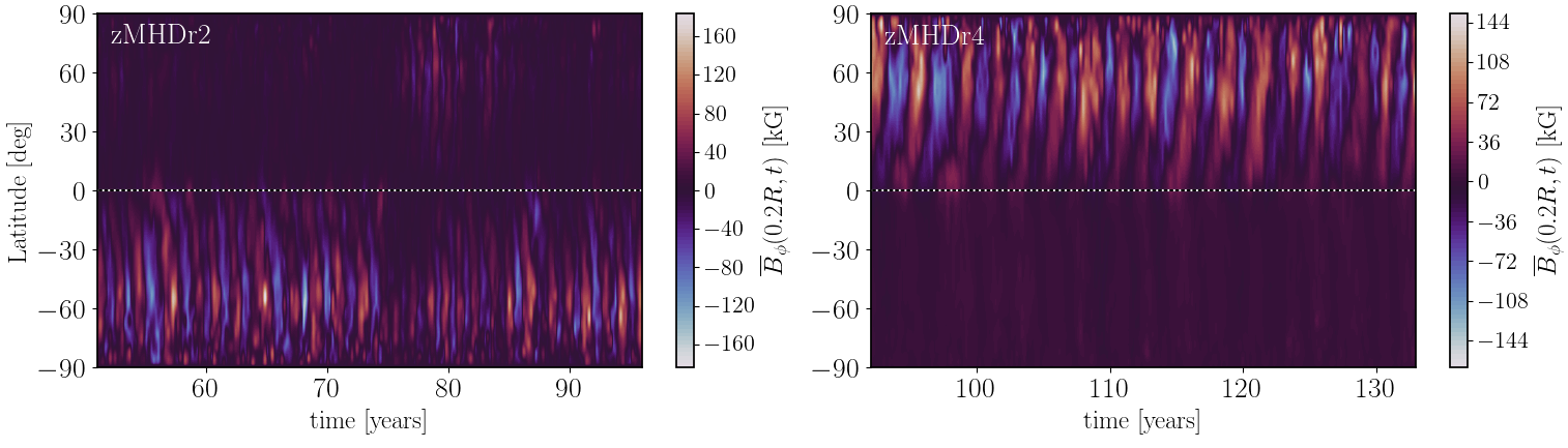
Figure 3: Same as Figure 2 but for the zoom models zMHDr2 and zMHDr4.

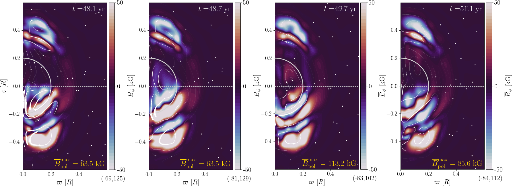
Figure 4: Azimuthally averaged toroidal magnetic field $\overline{B}_{\phi}(\varpi,z)$ from one cycle ($\sim$ 3 years) of MHDr3*. The poloidal magnetic field is represented with arrows, where the width is proportional to the strength of the field. The values of $\overline{B}_{\phi}$ are clipped to $\pm 50$ kG, and the maximum and minimum values $(\overline{B}_{\phi}^{\mathrm{min}},\overline{B}_{\phi}^{\mathrm{max}})$ are indicated below the colorbar. The dashed line at $z=0$ represents the equator.

The azimuthally averaged toroidal magnetic fields at $r=0.2R$ as functions of time and latitude of the full star simulations are shown in Figure 2. All of the magnetic field solutions are cyclic and hemispheric. These are the first cyclic solutions reported from core dynamos of early-type stars. Cyclic solutions have been reported in simulations of fully convective stars where the geometry of the dynamo region is similar to that of the current models with similar Coriolis number, $\mathrm{Co\approx 9}$ (Käpylä, 2021; Ortiz-Rodríguez et al., 2023). The main difference is the hemispheric nature of the current simulations, although during limited periods a run in Käpylä (2021) shows a predominantly hemispheric magnetic field as well (see their Fig. 10). Here, all the simulations show hemispheric fields most of the running time, with equally strong fields on both hemispheres only rarely (in particular Runs MHDr2, MHDr4* and zMHDr2). Hemispheric dynamo solutions have been also found in Boussinesq Landeau & Aubert (2011); Simitev & Busse (2012) and anelastic spherical shells models Raynaud et al. (2014); Raynaud & Tobias (2016). In Runs MHDr2 and MHDr3 the magnetic field is concentrated in the southern hemisphere, while in MHDr4 the magnetic activity is located in the northern hemisphere. In MHDr2*, the magnetic field starts in the southern hemisphere, same as in MHDr2, but then it moves to the northern hemisphere. This is a unique behaviour in this run and it is unclear why it happens. Similar behaviour was also found by Brown et al. (2020) in spherical simulations of fully convective M dwarfs, with no conclusive explanation either. The rest of the MHD* runs are very similar to their MHD counterparts, as shown in Figure 2. The dynamo of MHDr3* is essentially the same as that of MHDr3. MHDr4* has a cyclic dynamo on both hemispheres in the early part of the simulation, but the activity in the southern hemisphere vanishes after $\sim 23$ years, and the resulting magnetic field is similar to MHDr4. Something similar was found by Brown et al. (2020), where their hemispheric dynamos are initially symmetric on both hemispheres, but after some time strong southern-hemisphere fields replace the original symmetric configuration. The rms-magnetic fields from group MHD* are somewhat weaker than in group MHD; see Table 2.

Figure 3 shows $\overline{B}_{\phi}(r=0.2R,\theta,t)$ for two of the zMHD runs. These dynamos are also very similar to their MHD group counterparts. zMHDr2 shows a dynamo in the southern hemisphere. However, roughly between 75 and 85 years, it exhibits some activity in the northern hemisphere as well, which slightly reduces the activity in the southern hemisphere. This behaviour is also somewhat more frequently visible in MHDr2, and it is possibly related with the switch of active hemisphere seen in MHDr2*. The activity is almost completely hemispherical in all of the other simulations in the zMHD group. The toroidal magnetic field of zMHDr3 is not shown because it is almost identical to its full star counterparts, although, the mean intensity is somewhat weaker. Fourth column of Table 2 shows that a similar trend is present in all of the zMHD runs, so that $B_{\mathrm{rms}}$ is about $10$ kG weaker than in the full star MHD counterparts. As mentioned, the dynamo from zMHDr4 is very similar to that of MHDr4. However, their magnetic cycles does not seem to match and $P_{\mathrm{cyc}}$ from zMHDr4 is significantly shorter (2.50 yr) than that of MHDr4 (3.14 yr). The strengths of the toroidal and radial magnetic fields at the surface of the convective core ($r=0.2R$) for the full star runs are $\overline{B}_{\phi}^{\mathrm{rms}}=30-37$ kG and $\overline{B}_{r}^{\mathrm{rms}}=16-19$ kG, while the zoom have $\overline{B}_{\phi}^{\mathrm{rms}}=18-24$ kG and $\overline{B}_{r}^{\mathrm{rms}}=9-13$ kG, respectively.

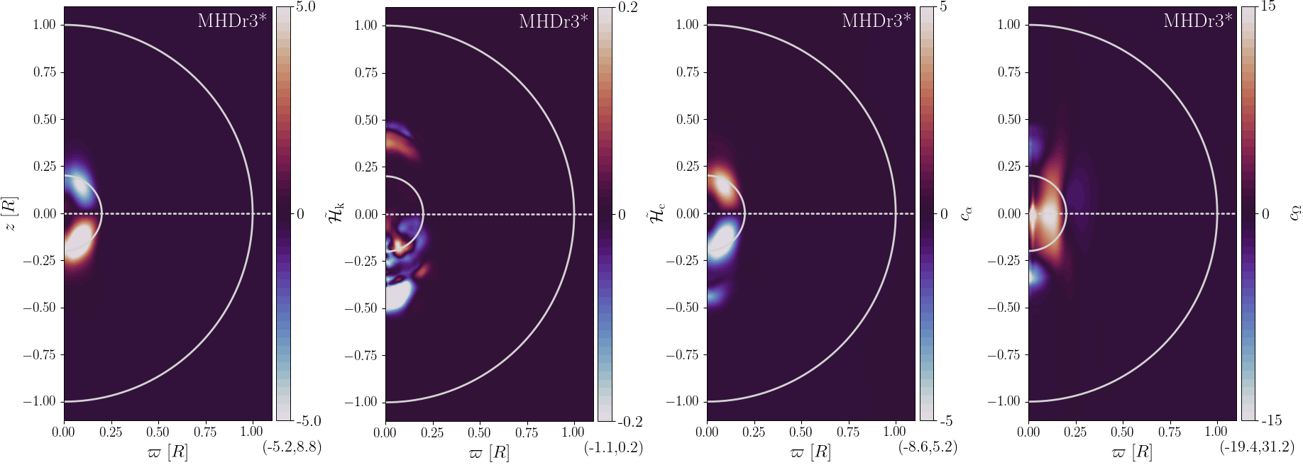
Figure 5: Time-averaged helicities and dynamo parameters from MHDr3*. From left to right the panels correspond to the normalised fluctuating kinetic helicity $\tilde{\mathcal{H}}_{\mathrm{k}}=\mathcal{H}_{\mathrm{k}}/(u_{\rm rms}^{2}/\Delta r)$, current helicity $\tilde{\mathcal{H}}_{\mathrm{c}}=\mathcal{H}_{\mathrm{c}}/(\rho_{0}u_{\rm rms}^{2}/\Delta r)$ helicities, and the dynamo parameters $c_{\alpha}=\alpha\Delta r/\eta_{\mathrm{t}}$ and $c_{\Omega}=\partial\overline{\Omega}/\partial r(\Delta r)^{3}/\eta_{\mathrm{t}}$. All the panels are clipped for better legibility.

The meridional distribution of the azimuthally averaged magnetic field of MHDr3* is shown in Figure 4. The amplitude of the mean toroidal component is typically larger than that of the mean poloidal component. In the core the full star runs have rms values of $\overline{B}_{\rm rms}^{\rm tor}$ = 20-25 kG and $\overline{B}_{\rm rms}^{\rm pol}$ = 18-22 kG, while the zoom models have $\overline{B}_{\rm rms}^{\rm tor}$ = 17-20 kG and $\overline{B}_{\rm rms}^{\rm pol}$ = 15-17 kG. Although the magnetic activity in the core is hemispheric, there is still some magnetic field in the radiative zone above the non-active hemisphere of the core. From Fig. 4, it is visible that this magnetic field might be coming from the core dynamo. At the beginning of the cycle ($t=48.1$ yr), the northern hemisphere of the core is almost free of magnetic activity. Briefly after, at $t=48.7$ yr, some of the magnetism from the core dynamo migrates through the northern hemisphere. This magnetism reaches the lower part of the radiative envelope while the core dynamo changes its polarity. Once the cycle finishes, the northern hemisphere of the core gets almost devoid of magnetic activity again. The zone where the magnetic field is concentrated in the radiative zone starts around $r\approx 0.6R$, which is roughly the radius where the radial jumps of the diffusivities occur in the MHD* group. Therefore, due to the low diffusivities in these layers, the magnetic field can stay and evolve in long timescales compared to the period of the core dynamo. These magnetic fields might be transported from the core to the bottom of the radiative envelope by the columnar flows produced by the Taylor-Proudman theorem, due to the high Coriolis numbers in our simulations (see Section 3.2). The reason of why these vertical flows can penetrate the stable stratification of the radiative envelope could be the unrealistically low Richardson number computed in such layers (see Table 2). These low values are a direct consequence of the low Brunt-Väisälä frequencies achieved by our simulations, as in real stars these values are expected to be several of orders of magnitudes higher. In the southern hemisphere the situation is similar, but the magnetic field has a different polarity than in the north.

To understand the origin of the dynamos in the simulations we make estimates of commonly used dynamo numbers in mean-field dynamo theory (e.g. Krause & Rädler, 1980). This involves computing the $\alpha$ effect which is proportional to the kinetic helicity of the flow (Steenbeck et al., 1966). The fluctuating kinetic and current helicities are

$$\mathcal{H}_{\mathrm{k}} =\overline{\bm{U}\bm{\cdot}\bm{\omega}}-\overline{\bm{U}}\bm{\cdot}\overline{\bm{\omega}}, \mathcal{H}_{\mathrm{c}} =\overline{\bm{J}\bm{\cdot}\bm{B}}-\overline{\bm{J}}\bm{\cdot}\overline{\bm{B}},$$ (27)

respectively, where $\bm{\omega}=\bm{\nabla}\times\bm{U}$ is the vorticity. Furthermore, to quantify the $\alpha$ and the $\Omega$ effects, it is convenient to introduce the following dynamo parameters (Käpylä et al., 2013)

$$c_{\alpha}=\frac{\alpha\Delta r}{\eta_{\mathrm{t}}},\hskip 14.22636ptc_{\Omega}=\frac{\partial\overline{\Omega}/\partial r(\Delta r)^{3}}{\eta_{\mathrm{t}}},$$ (28)

where $\eta_{\mathrm{t}}=\tau u^{2}_{\mathrm{rms}}/3$ is an estimate of the turbulent diffusivity and $\tau=\Delta r/u_{\mathrm{rms}}$ is the convective turnover time. Furthermore, the non-linear $\alpha$ effect is given by (Pouquet et al., 1976)

$$\alpha=-\frac{\tau}{3}\left({\cal H}_{k}-{\cal H}_{c}/\overline{\rho}\right).$$ (29)

Finally, $\overline{\Omega}$ is the time- and azimuthally-averaged rotation rate.

The normalized fluctuating kinetic helicity $\tilde{\mathcal{H}}_{\mathrm{k}}=\mathcal{H}_{\mathrm{k}}/(u_{\rm rms}^{2}/\Delta r)$ and current helicity $\tilde{\mathcal{H}}_{\mathrm{c}}=\mathcal{H}_{\mathrm{c}}/(\rho_{0}u_{\rm rms}^{2}/\Delta r)$ of MHDr3*, as well as the dynamo parameters (28) are shown in Figure 4. The kinetic helicity is negative (positive) in the northern (southern) hemisphere. The current helicity has a less well defined large-scale structure and a much lower amplitude. Along with the solar-like differential rotation of the core, which is discussed in Section 3.2, poleward propagation of dynamo waves is expected in the $\alpha\Omega$ dynamo approximation (e.g. Parker, 1955; Yoshimura, 1975). This is consistent with Figures 2 and 4. Furthermore, as shown in the rightmost panels of Figure 5, the values of $c_{\Omega}$ inside the core, are larger than those of $c_{\alpha}$. Although the difference between $\overline{B}_{\rm rms}^{\rm tor}$ and $\overline{B}_{\rm rms}^{\rm pol}$ is not very large, we nevertheless interpret the dynamos in our simulations to be of some $\alpha\Omega$ or $\alpha^{2}\Omega$ flavour. We note that $c_{\alpha}$ is close to zero at the base of the radiative zone between $z=0.25R$ and $z=0.5R$, which suggests lack of dynamo action there. In the southern hemisphere between $z=-0.5R$ and $z=-0.25R$, $c_{\alpha}$ has non-zero values, but these do not overlap significantly with the non-zero values of $c_{\Omega}$, suggesting dynamo action unlikely as well. Therefore, the interpretation that the magnetic field in the radiation zone, as seen in Figure 4, is transported there from the core dynamo remains plausible. The rest of the simulations have very similar kinetic helicity and dynamo coefficient profiles regardless of the location of the core dynamo.

Magnetic helicity conservation has profound consequences for large-scale dynamos. If magnetic helicity cannot exit the system, the $\alpha$ effect can be catastrophically quenched leading to resistively slow large-scale magnetic field growth (e.g. Brandenburg, 2001). In solar-like stars the dynamo-active region can shed magnetic helicity to the surrounding interstellar space via coronal mass ejections and other eruptive events. No such possibility exists for massive stars where the core dynamo is isolated from the stellar surface. A plausible possibility in this case is a diffusive magnetic helicity flux toward the equator where oppositely signed helicity can cancel. Such scenario has been demonstrated in simpler forced turbulence simulations where the kinetic helicity changes sign at the equator similarly as in the current models (e.g. Mitra et al., 2010). However, we postpone further investigation of this issue to future studies.

3.1.2 Surface magnetic fields

Figure 6: Time averaged rms magnetic field at the surface of the star $r=R$ as a function of latitude from the runs in groups MHD and MHD*.

Figure 6 shows the rms magnetic field $B_{\mathrm{rms}}$ at the surface of the star for the MHD and MHD* simulations. As expected, the magnetic field generated by the core dynamo is unable to create strong large-scale magnetic structures at the surface of the star. In all simulations the magnetic field is nearly zero on almost the whole surface of the star, except at the poles. The $B_{\mathrm{rms}}$ from latitudes between $-90$ and $-75$ degrees and from $75$ to $90$ degrees, that is near the poles, have the order of $0.1$ kG in the MHD group, and $10^{-3}$ kG in the MHD* group. While the magnetic fields from the rest of latitudes in both groups have values of the order of $10^{-5}$ kG. Additionally, there does not seem to be any correlation between the amount of magnetic flux that reaches the surface and the rotation period of the star. The highest rms value averaged over the poles in the MHD group comes from MHDr3 with $0.47\leavevmode\nobreak\ \mathrm{kG}$, and in the MHD* group from MHDr3*, with $6.8\cdot 10^{-3}\leavevmode\nobreak\ \mathrm{kG}$. Similarly to what happens in the bottom radiative envelope, the magnetic field are probably transported from the core to the surface near the poles by the combination of unrealistic Richardson numbers and axially aligned flows due to the high rotation of the simulations.

Although the radial profiles of the diffusivities in the MHD* group reduce the intensity of these flows and therefore, the magnetic field in the poles, they are still two orders of magnitude stronger than the magnetic fields in the rest of the stellar surface. In principle, increasing the Brunt-Väisälä frequency closer to realistic values should reduce the spreading of flows from the core to the envelope (see e.g. Korre & Featherstone, 2024). However, increasing this frequency is numerically very expensive, therefore with the current resolution of our simulations these results at the stellar surface should be taken with caution.

Finally, the magnetic field that reaches the poles is not only located at the pole corresponding to the active hemisphere despite the hemispheric nature of the core dynamo. This can be a consequence of the distribution seen in Fig. 4, as the flows might be transporting a fraction of the magnetic flux from the base of the bottom radiative envelope. The local rms velocity $u_{\mathrm{rms}}(\varpi,z)$ averaged from $\varpi=0$ to $\varpi=0.2R$, that is, close to the axis of rotation, has comparable values from $z=0.2R$ to $z=R$ and from $z=-0.2R$ to $z=-R$. Therefore a fraction of the magnetic field in the radiative zone seen in Fig. 4 is transported to the corresponding pole. From Fig. 6 is visible that the pole over the inactive hemisphere has a $B_{\mathrm{rms}}$ typically an order of magnitude weaker than that of the other pole, but it is still significantly higher than the rest of latitudes. The relatively high values of $u_{\mathrm{rms}}(\varpi,z)$ close to the axis of rotation are likely due to the combination of much higher diffusion coefficients and lower Richardson number in our simulations than in real stars. The advection timescales of the vertical flows are estimated to be around 100 yrs in the MHD group and 300 yrs in the MHD* group, while diffusion timescales are around $20$ yrs in both groups. Therefore, the magnetic field is transported to the surface most likely due to turbulent diffusion.

3.2 Large-scale flows

The time- and azimuthally-averaged rotation rate is given by:

$$\overline{\Omega}(\varpi,z)=\Omega_{0}+\overline{U}_{\phi}(\varpi,z)/\varpi,$$ (30)

where $\varpi=r\sin\theta$ is the cylindrical radius. Furthermore, the averaged meridional flow is:

$$\overline{\bm{U}}_{\mathrm{mer}}(\varpi,z)=(\overline{U}_{\varpi},0,\overline{U}_{z}).$$ (31)

We use the same parameters as in Käpylä et al. (2013), Käpylä (2021), and Ortiz-Rodríguez et al. (2023) to quantify the amplitude of the radial and latitudinal differential rotation. These are given by:

$$\Delta_{\Omega}^{(r)} =\frac{\overline{\Omega}(r_{\mathrm{top}},\theta_{\mathrm{eq}})-\overline{\Omega}(r_{\mathrm{bot}},\theta_{\mathrm{eq}})}{\overline{\Omega}(r_{\mathrm{top}},\theta_{\mathrm{eq}})},$$ (32)

$$\Delta_{\Omega}^{(\overline{\theta})} =\frac{\overline{\Omega}(r_{\mathrm{top}},\theta_{\mathrm{eq}})-\overline{\Omega}(r_{\mathrm{top}},\overline{\theta})}{\overline{\Omega}(r_{\mathrm{top}},\theta_{\mathrm{eq}})},$$ (33)

where $r_{\mathrm{top}}=0.9R$ and $r_{\mathrm{bot}}=0.1R$ are the radius near the surface and centre of the star, respectively. $\theta_{\mathrm{eq}}$ corresponds to the latitude at the equator, and $\overline{\theta}$ is an average of $\overline{\Omega}$ between latitudes $-\theta$ and $\theta$. Additionally, it is relevant to also analyse the differential rotation of the convective core. Therefore, we introduce $\Delta_{\Omega}^{\mathrm{CZ}(r)}$ and $\Delta_{\Omega}^{\mathrm{CZ}(\overline{\theta})}$, which are the same as (32) and (33), but with $r_{\mathrm{top}}=0.2R$ and $r_{\mathrm{bot}}=0.05R$.

Table 2: Differential rotation parameters and the maximum meridional flow $\overline{U}_{\mathrm{mer}}^{\mathrm{max}}$ from all simulations.

Run	$\Delta_{\Omega}^{(r)}$	$\Delta_{\Omega}^{(\overline{\theta})}(60^{\circ})$	$\Delta_{\Omega}^{(\overline{\theta})}(75^{\circ})$	$\Delta_{\Omega}^{\mathrm{CZ}(r)}$	$\Delta_{\Omega}^{\mathrm{CZ}(\overline{\theta})}(60^{\circ})$	$\Delta_{\Omega}^{\mathrm{CZ}(\overline{\theta})}(75^{\circ})$	$\overline{U}_{\mathrm{mer}}^{\mathrm{max}}\leavevmode\nobreak\ \mathrm{[m/s]}$
MHDr1	0.1579	-0.0001	-0.0011	0.3801	0.2650	0.4073	7.7
MHDr2	0.0505	-0.0001	-0.0006	0.1131	0.0699	0.1142	6.0
MHDr2*I	0.0405	-0.0001	-0.0007	0.0941	0.0607	0.0937	3.2
MHDr2*II	0.0538	-0.0000	-0.0006	0.1209	0.0734	0.1265	3.3
MHDr3	0.0251	-0.0000	-0.0004	0.0538	0.0295	0.0484	3.2
MHDr3*	0.0224	-0.0001	-0.0006	0.0489	0.0283	0.0438	2.1
MHDr4	0.0197	-0.0000	-0.0003	0.0405	0.0213	0.0350	2.5
MHDr4*	0.0169	-0.0001	-0.0006	0.0387	0.0208	0.0333	2.3
zMHDr1	-	-	-	0.3742	0.2442	0.3729	7.8
zMHDr2	-	-	-	0.1290	0.0739	0.1294	6.4
zMHDr3	-	-	-	0.0511	0.0282	0.0440	4.4
zMHDr4	-	-	-	0.0434	0.0214	0.0377	2.7

The differential rotation parameters are summarised in Table 2. From columns two to four of Table 2, we can conclude that the stellar surface rotates nearly rigidly, because $|\Delta_{\Omega}^{\overline{\theta}}|$ is $\sim 10^{-4}$ for $\theta=60^{\circ}$ and $\theta=70^{\circ}$. This implies negligible difference between the averaged rotation at the chosen latitudes and the equator. Figure 7 shows that in run MHDr3*, rigid rotation extends from the surface to a significant part of the radiative envelope between $r\approx 0.5R$ and $r=R$. This is similar to the radiative interior of the Sun, which has approximately rigid rotation (see Howe 2009). This behaviour is present in all the simulations from this study. Unlike the simulations by Augustson et al. (2016) whose radiative envelopes are almost completely rigid (see their Fig. 7), the current runs show a stronger differential rotation in the regions closest to the core.

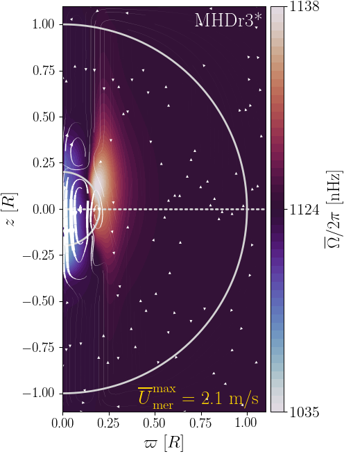
Figure 7: Profile of the temporally and azimuthally averaged rotation rate $\overline{\Omega}(\varpi,z)$ for MHDr3*. The streamlines indicate the mass flux due to meridional circulation and the maximum averaged meridional flow is indicated in the lower right side of the plot. The dashed line represents the equator.

All runs have positive $\Delta_{\Omega}^{(r)}$ because the innermost part of the core is rotating slower than the stellar surface, as shown in Figure 7. In Figure 8 the rotation profiles of other representative simulations are shown. The radial extent is now limited to $0.5R$, allowing a better display of the flows from the core and the portion of the radiative envelope with non-rigid rotation. The convective cores from all the runs have solar-like differential rotation, similar to the solar-like state reported by Brown et al. (2020), and the hydrodynamic case H4 of Augustson et al. (2016). This is also shown by the positive values of $\Delta_{\Omega}^{\mathrm{CZ}(\overline{\theta})}$ in Table 2, which indicate that the convective core is rotating faster at the equator than at other latitudes. Furthermore, we can see vertical structures that are parallel to the axis of rotation due to the Taylor-Proudman theorem. This is similar to the fast rotator from Brun et al. 2005 (see their Fig. 9). As mentioned in Section 3.1.2, these flows penetrate the radiative zone probably as a consequence of the low Brunt-Väisälä frequencies in our simulations. We estimate that ${\rm Ri}_{\Omega}$ in a real A0 star is of the order of $10^{4}$ which is five to six orders of magnitude higher than in the current simulations (see the tenth column in Table 2). Higher values of $N$ would also increase the ratio between the Eddington-Sweet and viscous timescales (e.g. Wood & Brummell, 2012), and the mean flows would only penetrate a small distance outside the core (see, e.g. Fig. 5 of Korre & Featherstone, 2024). Therefore, although high rotation rates influence the efficiency of angular momentum transport in massive stars (Aerts et al., 2019), we would not expect differential rotation to spread in such a significant part of the radiative envelope if realistic stellar parameters were used.

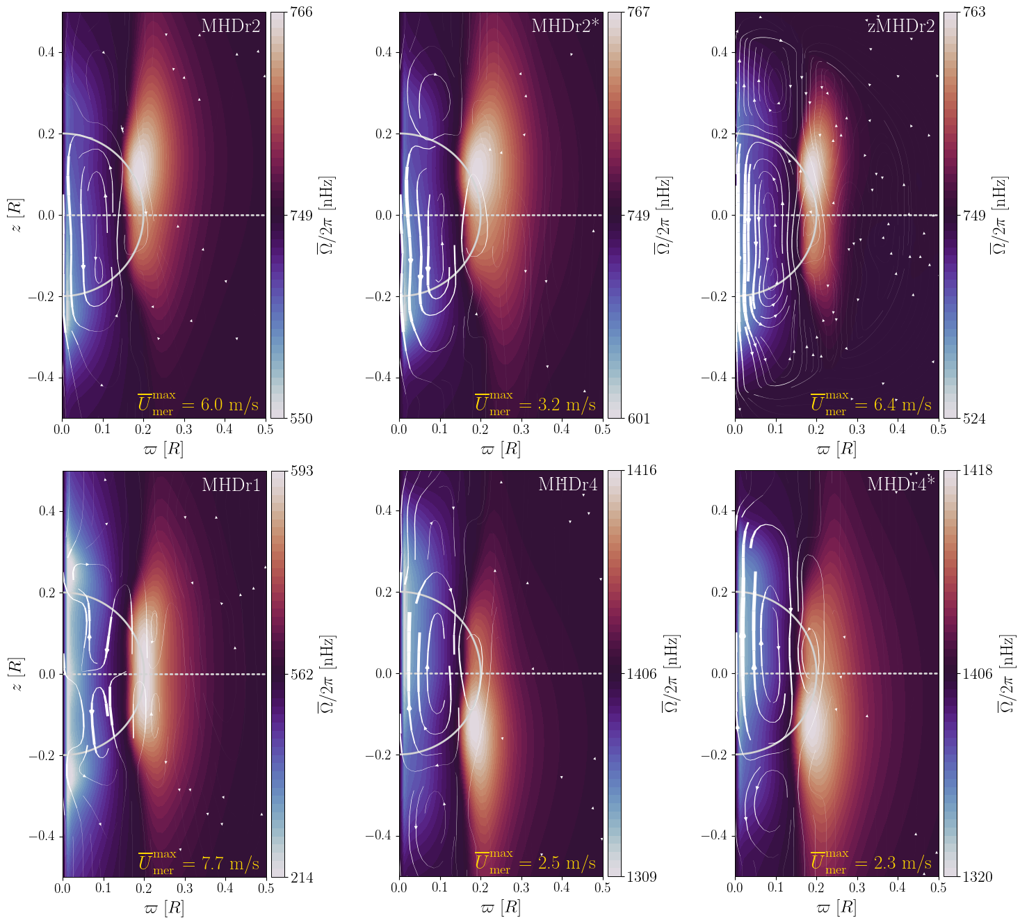
Figure 8: Profiles of the temporally and azimuthally averaged rotation rate $\overline{\Omega}(\varpi,z)$ of selected runs from all sets (clipped at $r=0.5R$). The upper panels show all the runs with $P_{\mathrm{rot}}=15\leavevmode\nobreak\ \mathrm{days}$ (MHDr2, MHDr2* and zMHDr2). The lower panels shows the run with no dynamo (MHDr1), and two simulations with $P_{\mathrm{rot}}=8\leavevmode\nobreak\ \mathrm{days}$ (MHDr4 and MHDr4*).

The Run MHDr1 without a dynamo has the largest differential rotation in the core; see columns five to seven in Table 2. The rotation profile is symmetric with respect to the equator; see the left lower panel of Figure 8. On the other hand, MHDr2 and MHDr4 are asymmetric with respect to the equator. This is due to the presence of strong hemispheric dynamos, which quench the differential rotation where the magnetic fields are strong. Magnetic quenching of differential rotation has been reported by various other numerical simulations (e.g. Brun et al., 2004; Käpylä et al., 2017; Bice & Toomre, 2023). Run MHDr3 behaves similarly to MHDr2. MHD* group shows similar behaviour. The rotation profile of MHDr2* shown in Figure 8 is averaged between 13 and 60 years, that is, before the dynamo moves from the southern to the northern hemisphere. As a consequence, the rotation profile is asymmetric with respect to the equator and very similar to that of MHDr2. After the dynamo migration ($t>60$ yrs) the rotation profile is inverted with respect to the equator and resembles that of MHDr4. The rest of the runs in the MHD* group are almost identical to their MHD counterparts, which is shown for Runs MHDr4* and MHDr4 in the lower panels of Figure 8. We note that the maximum meridional velocities $\overline{U}_{\mathrm{mer}}^{\mathrm{max}}$ are always smaller in the MHD* group (see last column of Table 2). Here the meridional flow amplitude is not monotonic in the rotation rate as the value of MHDr4* is slightly higher than that of MHDr3*, whereas in the MHD group the meridional flow amplitude decreases with increasing rotation rate.

The rotation profiles from group zMHD are very similar to their MHD counterparts, with similar maximum and minimum values of $\overline{\Omega}/2\pi$, and slightly higher maximum values of the averaged meridional flow, as shown for zMHDr2 in the upper right panel of Figure 8. zMHDr1 has $\overline{U}_{\mathrm{mer}}^{\mathrm{max}}=7.8\leavevmode\nobreak\ \mathrm{m/s}$ being the highest value of the simulations. In the rotation profile of zMHDr2, we can clearly distinguish more structures than in that of MHDr2. This is due to the increase of grid points inside the convective core, allowing to resolve flows on smaller scales. The same happens with all the runs from the zMHD group, but the main results remain the same, and therefore they are not included in the plot. In this set of simulations $\overline{U}_{\mathrm{mer}}^{\mathrm{max}}$ decreases with increasing $\Omega_{0}$, similar to the MHD group.

3.3 Energy analysis

3.3.1 Global and core energies

The total kinetic and magnetic energies, respectively, are given by

$$E_{\mathrm{kin}} =\frac{1}{2}\int\rho\bm{U}^{2}dV, E_{\mathrm{mag}} =\frac{1}{2\mu_{0}}\int\bm{B}^{2}dV.$$ (34)

The energies for the differential rotation (DR) and meridional circulation (MC), are

$$E_{\mathrm{kin}}^{\mathrm{DR}} =\frac{1}{2}\int\rho\overline{U}_{\phi}^{2}dV, E_{\mathrm{kin}}^{\mathrm{MC}} =\frac{1}{2}\int\rho(\overline{U}_{\varpi}^{2}+\overline{U}_{z}^{2})dV.$$ (35)

Furthermore, the toroidal and poloidal magnetic energies are defined as

$$E_{\mathrm{mag}}^{\mathrm{tor}} =\frac{1}{2\mu_{0}}\int\overline{B}_{\phi}^{2}dV, E_{\mathrm{mag}}^{\mathrm{pol}} =\int\frac{1}{2\mu_{0}}(\overline{B}_{\varpi}^{2}+\overline{B}_{z}^{2})dV.$$ (36)

These expressions (34-36) were integrated over the volume of the star ($r<R$), or over the convective core ($r<\Delta r$), to study the energies in the entire star and in core, respectively. The obtained values are listed in Table 3.

Table 3: Kinetic and magnetic energies.

Run	$E_{\mathrm{kin}}\leavevmode\nobreak\ [10^{33}\mathrm{J}]$	$E_{\mathrm{kin}}^{\mathrm{DR}}/E_{\mathrm{kin}}$	$E_{\mathrm{kin}}^{\mathrm{MC}}/E_{\mathrm{kin}}$	$E_{\mathrm{mag}}\leavevmode\nobreak\ [10^{33}\mathrm{J}]$	$E_{\mathrm{mag}}/E_{\mathrm{kin}}$	$E_{\mathrm{mag}}^{\mathrm{tor}}/E_{\mathrm{mag}}$	$E_{\mathrm{mag}}^{\mathrm{pol}}/E_{\mathrm{mag}}$
Full star
MHDr1	296.78	0.631	0.017	-	-	-	-
MHDr2	74.50	0.398	0.017	24.00	0.322	0.294	0.061
MHDr2*	74.70	0.391	0.018	24.71	0.331	0.277	0.059
MHDr3	42.57	0.319	0.011	23.99	0.563	0.229	0.079
MHDr3*	43.81	0.315	0.010	30.52	0.697	0.264	0.074
MHDr4	34.86	0.323	0.008	23.79	0.682	0.300	0.086
MHDr4*	35.84	0.317	0.006	26.58	0.742	0.266	0.069
Core
MHDr1	32.64	0.576	0.025	-	-	-	-
MHDr2	8.88	0.346	0.026	1.74	0.196	0.140	0.097
MHDr2*	8.95	0.341	0.027	1.56	0.174	0.132	0.098
MHDr3	5.10	0.286	0.016	2.06	0.403	0.151	0.112
MHDr3*	4.91	0.247	0.016	1.86	0.379	0.139	0.102
MHDr4	4.19	0.309	0.011	1.74	0.415	0.189	0.118
MHDr4*	3.96	0.259	0.009	1.58	0.399	0.172	0.108
zMHDr1	27.47	0.537	0.032	-	-	-	-
zMHDr2	9.00	0.371	0.035	1.20	0.133	0.133	0.091
zMHDr3	4.61	0.275	0.021	1.40	0.304	0.152	0.102
zMHDr4	3.83	0.331	0.014	1.06	0.277	0.186	0.104

The slowest rotators have the highest kinetic energies and $E_{\rm kin}$ decreases with $\Omega_{0}$. This is a consequence of high rotation rates reducing the intensity of the flows, as visible from $u_{\mathrm{rms}}$ in Table 2 and the differential rotation parameters in Table 2. We note that MHDr1 has a significantly higher value of $E_{\mathrm{kin}}$ than the rest of the simulations, which is a consequence of the absence of dynamo in this run. Earlier simulations (e.g. Brown et al., 2008; Viviani et al., 2018) and theoretical considerations (e.g. Kitchatinov & Rüdiger, 1999) suggest that differential rotation and meridional circulation decrease when the rotation rate increases. Our results are mostly in agreement with these results, although the most rapidly rotating runs in each group deviate from this trend. A possible explanation is that the flows penetrate deeper in the radiative layer in these simulations due to the higher rotation rate and smaller Richardson numbers.

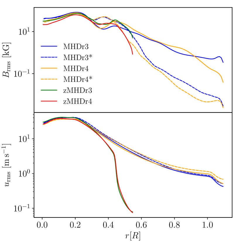
Figure 9: Radial profiles of the horizontally averaged $B_{\mathrm{rms}}$ (top panel) and $u_{\mathrm{rms}}$ (bottom panel) from representative runs.

The magnetic and kinetic energies of the entire star are always larger in the group MHD* than in group MHD. This is because of the different diffusivity profiles between groups. In Figure 9 is visible from the $B_{\mathrm{rms}}$ profile that runs from group MHD* have a secondary maxima closer to the core than those of group MHD. These maxima above the core envelope interface around $0.36R$ lead to higher overall values of $B_{\mathrm{rms}}$ in the MHD* group even though the fields in the radiative envelope are weaker in these cases. However, this behavior disappears in the core, as shown in the last rows of Table 3. With $r<\Delta r$ the values of the magnetic energy in group MHD* are smaller than in group MHD, while the values of the kinetic energy, although quite close, do not seem to show any tendency between groups. Similarly to the differential rotation energies, the toroidal magnetic energies are very similar, with values of $E_{\mathrm{mag}}^{\mathrm{tor}}/E_{\mathrm{mag}}$ between 0.229 and 0.3 for $r<R$, and between 0.132 and 0.189 for $r<\Delta r$. In both cases, the highest value occurs in MHDr4, same as with the poloidal magnetic energy. However, the maximum $E_{\mathrm{mag}}$ occurs in MHDr3* for the entire star, and in MHDr3 for the core. This is consistent with Table 2, as these runs show the highest $B_{\mathrm{rms}}$. In the core, toroidal magnetic energies are somewhat larger than the poloidal energies, with typically $E_{\mathrm{mag}}^{\rm tor}\approx 1.5E_{\mathrm{mag}}^{\rm pol}$. This is consistent with the discussion about the nature of the core dynamo; see Section 3.1.1.

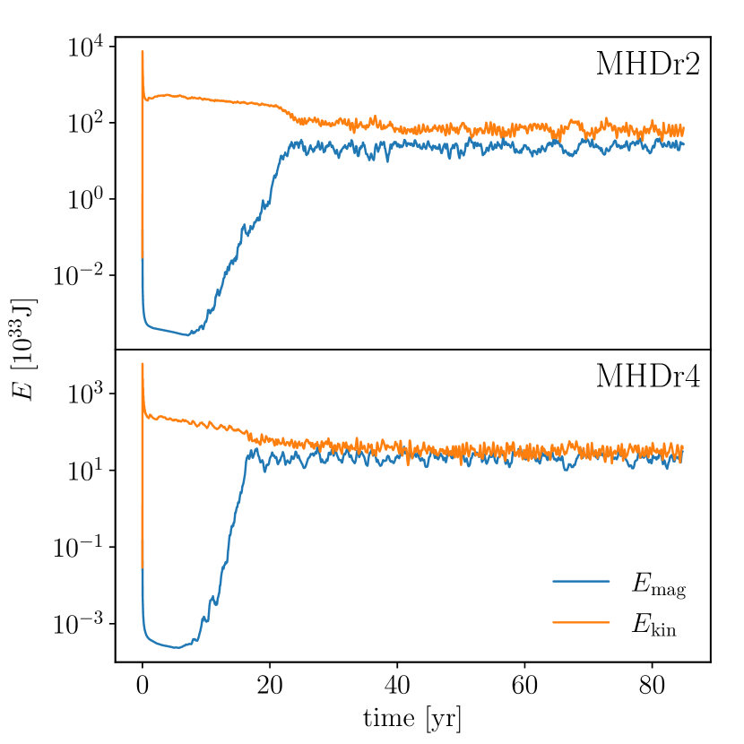
Figure 10: Temporal evolution of the magnetic (blue) and kinetic (orange) energies in the full star of the runs MHDr2 (top panel) and MHDr4 (bottom panel).

The magnetic energies in all of the current simulations are below equipartition even in the most rapidly rotating cases, typically with $E_{\mathrm{mag}}/E_{\mathrm{kin}}\approx 0.4$, and only when considering the energies in the whole star the magnetic energy is near or at equipartition; see Fig. 10. We therefore do not reach the near equipartition regime in the dynamo region that was found by Brun et al. (2005). This is likely because of the relatively laminar parameter regime explored in the current study. The kinetic energies in the zMHD group are comparable to the corresponding full star runs. However, as with $B_{\mathrm{rms}}$, the total magnetic energy in the zMHD runs are lower than in the rest of simulations.

3.3.2 Energy fluxes and luminosities

The luminosities related to the radiative, enthalpy, kinetic energy, and viscous fluxes, and the additional cooling and heating, are defined as (Käpylä, 2021):

$$\mathscr{L}_{\mathrm{rad}} =-4\pi r^{2}\langle K\rangle_{\theta\phi t}\frac{\partial\langle T\rangle_{\theta\phi t}}{\partial r}, \mathscr{L}_{\mathrm{enth}} =4\pi r^{2}c_{\mathrm{P}}\langle(\rho U_{r})^{\prime}T^{\prime}\rangle_{\theta\phi t},$$ (37)

$$\mathscr{L}_{\mathrm{kin}} =2\pi r^{2}\langle\rho\bm{U}^{2}U_{r}\rangle_{\theta\phi t}, \mathscr{L}_{\mathrm{visc}} =-8\pi r^{2}\nu\langle\rho U_{i}\mathsf{S}_{ir}\rangle_{\theta\phi t},$$ (38)

$$\mathscr{L}_{\mathrm{cool}} =-\int_{0}^{r}4\pi r^{2}\langle\mathcal{C}\rangle_{\theta\phi t}dr, \mathscr{L}_{\mathrm{heat}} =\int_{0}^{r}4\pi r^{2}\langle\mathcal{H}\rangle_{\theta\phi t}dr,$$ (39)

where primes indicates fluctuations from the horizontal ($\theta\phi$) average, $r$ denotes the radial component in spherical coordinates, and $\langle.\rangle_{\theta\phi t}$ horizontal and temporal averaging.

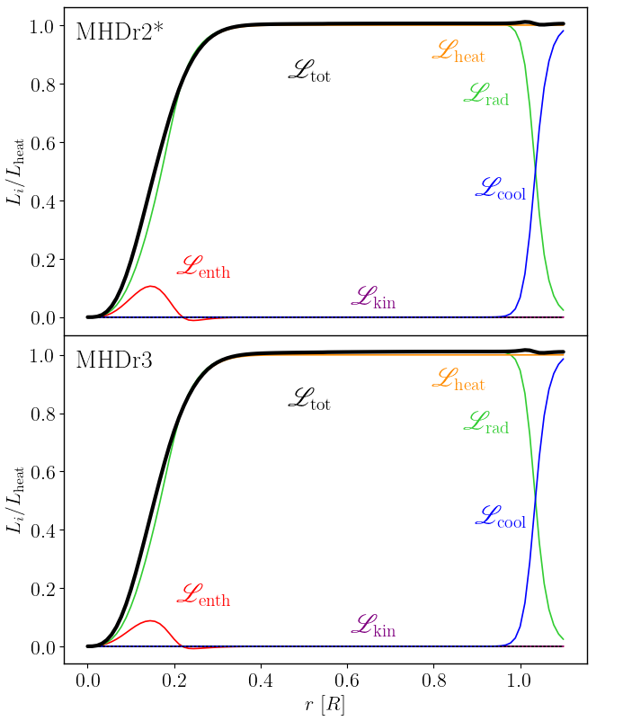
Figure 11: Luminosity contributions from kinetic energy, enthalpy, radiative, cooling and heating fluxes from MHDr2* (top panel) and MHDr3 (bottom panel).

The contributions to the total luminosity from runs MHDr3 and MHDr2* are shown in Figure 11. $\mathscr{L}_{\mathrm{visc}}$ is not shown because it is negligible, reaching maximally $0.02\%$ of the total flux at $r\approx 0.22R$. The convective luminosity $\mathscr{L}_{\mathrm{conv}}=\mathscr{L}_{\mathrm{kin}}+\mathscr{L}_{\mathrm{enth}}$ is dominated by a positive $\mathscr{L}_{\mathrm{enth}}$ in the convection zone ($0<r\leq 0.2R$). The kinetic energy flux is negligible which is expected in the rapid rotation regime; see, for example Käpylä (2024). In the majority of the star, the contribution due to the radiative energy flux dominates. This is due to the internal structure of the star, where the main energy transfer mechanism is radiation (the radiative zone is roughly $80\%$ of the radial extent). Near the surface of the star the cooling becomes effective and it dominates the total luminosity. The rest of the runs from groups MHD and MHD* have almost identical luminosity profiles. These profiles are similar to those of Augustson et al. (2016) and Brun et al. (2005), see their Figs. 3 and 13, respectively. The contribution of $\mathscr{L}_{\mathrm{enth}}$ in the core is about $10\%$ which is somewhat smaller than in Brun et al. (2005) ($\approx 25\%$), and in Augustson et al. (2016) ($\approx 40\%$). In the zMHD group the luminosity profiles are very similar to those shown in Figure 11, with the obvious differences that these profiles extend only to $r=0.55R$ and the cooling becomes effective around $r=0.5R$.

3.4 Rotational scaling of magnetic cycles

Table 4: Comparison of values of $\beta$.

Data	Sample	$\beta$	References
Late-type stars observations	Active branch	$0.48$	Brandenburg et al. (1998)
	Inactive branch	$0.46$
	S branch	-0.43	Saar & Brandenburg (1999)
	45 FGK stars	$<0$	Boro Saikia et al. (2018)
	15 M dwarfs	$-1.02\pm 0.06$	Irving et al. (2023)
	40 FGK stars	$-0.81\pm 0.17$
Solar-like stars simulations	Slow rotators	$-0.73$	Viviani et al. (2018)
	Fast rotators	$-0.50$
	Global fit	$-0.99\pm 0.05$	Warnecke (2018)
	Global fit	$-1.58\pm 0.11$	Strugarek et al. (2018)
	Slow rotators	$-0.47\pm 0.15$	Guerrero et al. (2019)
	Fast rotators	$1.17\pm 0.05$
	Surface cycles	$-0.03\pm 0.12$	Käpylä (2022)
	Deep cycles	$-0.11\pm 0.17$
M dwarf simulations	Global fit	$-1.30\pm 0.26$	Ortiz-Rodríguez et al. (2023)
A-type star simulations	MHD group	$-1.22\pm 0.05$	Present work
	MHD* group	$-1.13\pm 0.11$
	zMHD group	$-0.83\pm 0.16$

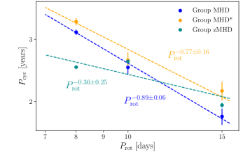
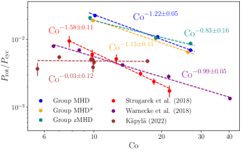
Figure 12: Left panel: The magnetic cycle period $P_{\mathrm{cyc}}$ as a function of the rotation period $P_{\mathrm{rot}}$. Right panel: Ratios of rotation to cycle period as a function of the Coriolis number. Additional data are from Strugarek et al. (2018, red), Warnecke (2018, purple) and Käpylä (2022, brown). The dashed lines are the best power-law fits to the data.

As discussed in Section 3.1.1, the averaged toroidal magnetic fields in the core show clear cycles. To estimate the magnetic cycle period $P_{\mathrm{cyc}}$ of the core dynamo we computed the spectral density of the magnetic field at different latitudes from the active hemisphere using Welch’s method (Welch, 1967). The peak value of the power spectrum corresponds to the frequency of the magnetic cycle, and its inverse gives the cycle period. The mean value of $P_{\mathrm{cyc}}$ obtained from the considered latitudes with the respective standard error is listed in the last column of Table 2. In the full star models there is a clear trend that $P_{\mathrm{cyc}}$ increases with decreasing $P_{\mathrm{rot}}$. This is visible in left panel of Figure 12. Furthermore, our best power-law fit shows $P_{\mathrm{cyc}}\propto P_{\mathrm{rot}}^{-0.89\pm 0.06}$ in the MHD group, and $P_{\mathrm{cyc}}\propto P_{\mathrm{rot}}^{-0.77\pm 0.16}$ in the MHD* group. The relation between the magnetic cycle of the core dynamo and rotation has not been studied before. However, simulations of solar-like stars have shown similar results. Data from Warnecke (2018) indicate $P_{\mathrm{cyc}}\propto P_{\mathrm{rot}}^{-1.06}$, which is a relation steeper than those found in our simulations. In the zMHD group the magnetic cycle period seems to be less sensitive to rotation. Our best fit shows $P_{\mathrm{cyc}}\propto P_{\mathrm{rot}}^{-0.36\pm 0.25}$, which is less steep than in the full star models. This relation is similar to the $P_{\mathrm{cyc}}\propto P_{\mathrm{rot}}^{-0.33\pm 0.05}$ reported in Strugarek et al. (2017).

Observations of chromospheric activity suggest that the stellar magnetic activity cycles are distributed in active and inactive branches (see e.g. Brandenburg et al., 1998; Böhm-Vitense, 2007). These studies suggest a relation $P_{\mathrm{rot}}/P_{\mathrm{cyc}}\propto\mathrm{Co}^{\beta}$ with $\beta>0$. However, the exact nature of these branches and the relation between stellar cycles and rotation are still under debate (e.g. Brandenburg et al., 2017; Boro Saikia et al., 2018; Bonanno & Corsaro, 2022). We present this relation in the core dynamo of an A-type star for the first time, with $\beta\approx-1$ in all the sets. Our results are shown in the right panel of Figure 12. Furthermore, our best power law fits are summarised in Table 4. Data from other authors from observations and numerical simulations is also added for comparison purposes. From Table 4 it is visible that our results are usually in agreement with solar-like simulations. However, as discussed in Section 3.1.1, the expulsion of the magnetic helicity has direct consequences in the cycle period, and the mechanism responsible is expected to differ between core and envelope dynamos. One possible explanation of why the scaling laws seem to agree, is that all the solar-like simulations reported in Table 3.1.1 have been done at relatively modest magnetic Reynolds numbers, therefore, the direct effects of the magnetic helicity conservation might not be immediately visible.

4 Summary and conclusions

We present results from star-in-a-box simulations (see Dobler et al., 2006; Käpylä, 2021) of a $2.2\leavevmode\nobreak\ M_{\odot}$ A-type star with a convective core of roughly $20\%$ of the stellar radius. We explore rotation periods from 8 to 20 days in three sets of simulations. The full star sets MHD and MHD* have somewhat different radial profiles of the kinematic viscosity and the magnetic diffusivity. The third set (zMHD) consists of zoom-in versions of the MHD group, where we model the convective core and a part of the radiative envelope at higher resolution. All of the core dynamos are hemispheric and cyclic with rms values of around 60 kG. Observational constrains of the internal magnetic field strength of early-type stars can be obtained via asteroseismology. Lecoanet et al. (2022) estimated an upper limit of $B_{r}\approx 500\leavevmode\nobreak\ \mathrm{kG}$ at $r=0.18R$ for the B star HD 43317, based on the g-mode frequencies from Buysschaert et al. (2018). Our results are one order of magnitude lower than this (at $r=0.20R$ we find $\overline{B}_{r}^{\mathrm{rms}}\approx 20$ kG). However, in B-type stars the convective velocities in the core are expected to be roughly ten times higher than in A-type stars (Browning et al., 2004). Therefore we would expect correspondingly stronger magnetic fields in the former; see, for example Augustson et al. (2016). The dynamos in our simulations remain hemispheric throughout the simulation time, except in MHDr2* where the magnetic activity migrated from the southern to the northern hemisphere. Similar behaviour was reported by Brown et al. (2020) in fully convective M drawfs but the reason behind it is not clear. Some magnetic fields reach the surface of the star in our simulations. However, these fields are very weak everywhere except at the poles, where the maximum rms value averaged over the poles ($-90^{\circ}>\theta>-75^{\circ}$, and $75^{\circ}<\theta<90^{\circ}$) is in run MHDr3 with $\sim 0.47$ kG. In the group MHD* the surface magnetic fields are significantly weaker due to the different radial profiles of diffusivities, with maximum values around $10^{-4}$ kG. These weak surface magnetic fields might be a consequence of the flows aligned with the rotation axis because of the Taylor-Proudman theorem, due to the high Coriolis numbers in our simulations. Such flows could penetrate the radiative layers due to the unrealistically low Richardson number there.

All the simulations have approximately rigid rotation in a significant part of their radiative envelope, and a solar-like differential rotation in the convective core. On average, the core is rotating slightly slower than the envelope. Run MHDr1 has $\overline{\Omega}(r=0.2R)/\overline{\Omega}(r=R)\approx 0.8$, while the runs with dynamos have ratios very close to unity. Differential rotation has been observed in early-type stars via asteroseismology (see Bowman, 2021, 2023, and the references therein). Kurtz et al. (2014) reported the surface-to-core rotation of the main-sequence A-type star KIC 11145123, finding that the star is almost a rigid rotator, but the surface rotates slightly faster than the core in agreement with our simulations. Furthermore, most of the observed intermediate-mass main-sequence stars have nearly rigid rotation, based on the average near-core and envelope rotation rates (see Fig. 4 of Bowman, 2023). In massive stars ($M>9M_{\odot}$), the near-core rotation rate is typically larger than that of the envelope. For example, recently, Burssens et al. (2023) deduced the core-to-surface radial rotation profile of the B star HD 192575, finding that the convective core is rotating between 1.4 and 6.3 times faster than the radiative envelope.

The hemispheric dynamos imprint an asymmetry also on the rotation profile via magnetic quenching of the the differential rotation. There is no clear difference between groups in their rotation profiles. As we increase the rotation rate, the magnetic energy gets closer to the equipartition values with the kinetic energy. The magnetic energy inside the core reaches $E_{\mathrm{mag}}\approx 0.4E_{\mathrm{kin}}$ in the fast rotators MHDr4 and MHDr4*, while in the full star both energies are comparable. None of our runs reached super-equipartition values like the fast rotators in Augustson et al. (2016). This might be a consequence of the different values of the dimensionless diagnostic parameters in their simulations, for example, the fluid Reynolds number (computed as $\mathrm{Re}^{\prime}/2\pi$ for a proper comparison, see Appendix A of Käpylä et al., 2017) are in the range of 81-132, while those in our study range between 25 and 52. Furthermore, $\mathrm{Re}_{\mathrm{M}}$ ($\mathrm{Rm^{\prime}}/2\pi$) in their work ranges from 324 to 490, being significantly higher than those in the current study (17-36).

All groups have very similar luminosity profiles, which are also similar to those in Brun et al. (2005) and Augustson et al. (2016). In general, the zoom models show very similar results compared to the full star models. However, in the zoom models the magnetic fields are slightly weaker (see Tables 2 and 3). This is possibly a resolution effect. Nevertheless, the changes are not drastic and the large-scale structures are very similar giving us confidence in the robustness of the results.

We find a relation $P_{\mathrm{cyc}}\propto P_{\mathrm{rot}}^{\alpha}$ with $\alpha=-0.89\pm 0.06$, $\alpha=-0.77\pm 0.16$ and $\alpha=-0.36\pm 0.25$ in the groups MHD, MHD* and zMHD, respectively. Furthermore, we present a scaling of $P_{\mathrm{rot}}/P_{\mathrm{cyc}}\propto\mathrm{Co}^{\beta}$, with $\beta=-1.22\pm 0.05$ in the MHD group, $\beta=-1.13\pm 0.11$ in the MHD* group and $\beta=-0.83\pm 0.16$ in the zMHD group, being the first time that this has been done with the core dynamo cycle of an A-type star. Similar results with $\beta\approx-1$ were recently reported by Irving et al. (2023) and have been found in data from simulations of other types of stars (e.g. Warnecke, 2018; Strugarek et al., 2018; Viviani et al., 2018; Ortiz-Rodríguez et al., 2023). Furthermore, Bonanno & Corsaro (2022) reported a dichotomy in the relation $P_{\mathrm{cyc}}\propto P_{\mathrm{rot}}^{\alpha}$, in terms of $\omega_{\mathrm{cyc}}=2\pi/P_{\mathrm{cyc}}$ and $\Omega=2\pi/P_{\mathrm{rot}}$, where our results ($\alpha<0$) agree with one of the reported branches (Group 2 in their Fig. 1). This branch is attributed to having older stars with higher metallicities than the other. The reason of why our simulations fit with this group is currently unclear. However, there is considerable debate regarding the scaling of stellar cycles as a function of rotation both from observations as well as simulations (see, e.g. Käpylä et al., 2023, and references therein).

Our simulations indicate that the magnetic field created by a core dynamo is not enough to explain the large-scale structures observed at the surface of Ap/Bp stars, in accordance with earlier analytical studies (e.g. MacGregor & Cassinelli, 2003). This makes sense considering the wide range of magnetic field strengths observed at the surfaces of stars whose convective cores are predicted to be of similar size. Moreover, the surface magnetic fields of Ap/Bp stars often have simple geometries, for example, dipoles with a magnetic axis misaligned with the rotational axis, supporting the fossil field theory (see Keszthelyi, 2023, and the references therein). Interesting, the internal magnetic field inferred by Lecoanet et al. (2022) seems to be unlikely to reach exclusively with fossil fields, supporting the evidence of a strong core dynamo inside early-type stars. In future studies, different mechanisms (for example, fossil fields, Tayler-Spruit dynamo) should be included while the strong core dynamo is present. A logical step to follow in the future is to add a fossil field into our model, and to study how these magnetic configurations affect the nature of the hemispheric dynamo that was obtained in all the magnetic runs. Different initial configurations can be implemented as a way to test their stability and how they interact with an existing core dynamo, similarly to Featherstone et al. (2009) but also modelling the entire star and seeing how the resulting magnetic field behaves at the stellar surface. Furthermore, more rotation rates can be explored, although it is true that Ap stars can rotate very slowly ($P_{\mathrm{rot}}=300$ years), most of them have rotation periods between 1 and 10 days (Braithwaite & Spruit, 2017), so the “fast rotator regime”, from 1 to 8 days, remains unexplored.