Finite-size effects in two-photon correlations of exciton Bose-Einstein condensates

Abstract

Accessing two-photon statistics via Hunbary Brown and Twiss (HBT)-type measurements is essential for investigations of excitonic Bose-condensates. In this paper we make use of quantum hydrodynamics in order to study the finite-size impact on the two-photon emission intensity of a 2D condensate of excitons. We use the developed approach to calculate the two-photon decay time of exciton condensate in GaAs quantum wells and MoS₂ bilayers. We demonstrate that the registered signal scales on the sample size in a qualitatively different manner than the Bogoliubov theory predicts.

I Introduction

Among the accessible experimental platforms for exploring Bose-condensation, excitons and excitonic polaritonic are, perhaps, the most attractive ones due to their strong interaction with light. This both facilitates their experimental investigations via spectroscopic measurements and implies promising applications of excitonic, polaritonic or even purely photonic condensates as coherent light sourcesByrnes et al. (2013); J.Klaers et al. (2010); Maximov et al. (2023a).

With optical measurements being the main experimental tool for identifying condensation and quantifying coherence of the emitted light, the key signature of condensate emergence is the multimode character of luminescence, manifested in nontrivial two-photon correlations. As implied by the classical Hanbury Brown and Twiss (HBT) experiment BROWN and TWISS (1956), photons demonstrate no bunching when being emitted from a single-mode light source (with Bose-Einstein condensate being an example) as opposed to the case of a chaotic (thermal) one.

Indeed, two-photon spectroscopy clearly distinguishes the condensed and the thermal states for both polaritonic Kasprzak et al. (2008); Tempel et al. (2012) and pure excitonic Gorbunov et al. (2009) gases, allowing experimental investigation of their phase diagrams. The increasing time resolution of two-photon spectroscopy made it possible to study dynamics of condensates. In particular, with the use of streak-cameras as photodetectors, which decreased the time-resolution up to a few ps Aßmann et al. (2010); Takemura et al. (2012), condensation kinetics became directly observable. Such a resolution is enough to study condensate decoherence Love et al. (2008) and even to access the relaxation dynamics of the polaritonic gas towards the BEC state Adiyatullin et al. (2015). In addition, among the novel techniques which provide both high time resolution and high sensitivity are the ones based on frequency upconversion in a nonlinear waveguide Delteil et al. (2019).

To describe the results of intensity correlation measurements, one has to study population build-up in a single mode, which may be qualitatively described even by the ideal Bose gas model. However, the quantitative differences due to particle interaction are significant Perrin et al. (2012). Moreover, especially in two dimensions, where thermal fluctuations are known to spoil long-range order Hohenberg (1967); Mermin and Wagner (1966), one has to carefully consider finite-size effects. In a finite two-dimensional semiconductor sample with polariton or exciton gas, one deals with a system with potentially highly depleted condensate due to both strong interactions Lozovik et al. (2007a) and diverging thermal fluctuations owing to reduced dimensionalityKane and Kadanoff (1967). In this regime the standard Bogoliubov theory (hereafter BT) is not applicable, which motivates the current work. The aim of our study is to utilize the quantum hydrodynamic approach unified with the BT Kane and Kadanoff (1967); Voronova et al. (2018); Grudinina et al. (2021) to evaluate the intensity of the two-photon radiation and to study its dependence on the system size.

The approach developed in this paper is quite general and may be applied to a variety of 2D systems, namely excitons and exciton polaritons in quantum wells as well as the ones in novel 2D materials, among which TMDCs attract much interest in the context of exciton coherence in recent yearsBrem et al. (2020); Brunetti et al. (2018); Wang et al. (2014); Tang et al. (2024).

In the following chapters we investigate the two-photon signal emitted by a BEC of excitons in a semiconductor microcavity. We start by describing a model experimental setup to detect the two-photon signal in Section II. Then follows the Section III with a detailed microscopic description of the excitonic system coupled to photonic modes of the environment. In Section IV we use techniques of many body physics in order to deduce an expression for the two-photon signal. Finally, we discuss the results with special emphasis on size-dependent features in Section V. We perform numerical calculations for excitons in a GaAs/AlGaAs/GaAs quantum wells and spatially indirect ones in MoS₂ bilayer. Moreover, we demonstrate how to apply our results to polaritonic condensates. Conclusions follow in Section VI.

II Experimental setup

For excitons in a 2D semiconductor sample of size $L\times L$, the two-photon emission intensity from unit area is as follows :

$$P_{\rm total}=\frac{\braket{N_{1}N_{2}}}{L^{2}t_{0}},$$

where $N_{1}$ and $N_{2}$ are the total number of photons emitted in two directions in a finite time interval $t_{0}$. The bracket $\braket{...}$ denotes the ensemble average:

$$\braket{N_{1}N_{2}} =\sum\limits_{\bm{p}\bm{p}^{\prime}}\operatorname{Tr}\left[\rho(t)\widehat{N}_{\bm{p}}\widehat{N}_{\bm{p}^{\prime}}\right].$$ (1)

Here the sum is over 3D momenta of emitted photons, $\rho(t)$ is the density matrix of the system under consideration (2D excitons (polaritons) + 3D environmental photons).

The presence of condensate manifests itself in a contribution to this sum of a sharp angularity. Namely, the one with opposite in-plane components of the emitted photons (for details see Appendix A). Using a decomposition $\bm{p}=\bm{q}+p_{z}\bm{e}_{z}$ with the two terms being the in-plane and out-of-plane components of the photon momentum respectively, we may isolate this contribution:

$$P_{\rm total}=\underbrace{\sum_{\bm{q}=\bm{q}^{\prime}}p_{\bm{q},\bm{q}^{\prime}}\delta(\bm{q}+\bm{q}^{\prime})}_{P_{\rm angled}}+\underbrace{\sum_{\bm{q}\neq\bm{q}^{\prime}}P_{\bm{q},\bm{q}^{\prime}}}_{P_{\rm background}}.$$ (2)

For detection of the angled contribution, we consider an experimental setup with two photon detectors $D_{1}$ and $D_{2}$ placed above the sample as depicted on Figure 1. They are in the same plane, which ensures $\bm{q}_{1}=-\bm{q}_{2}$.

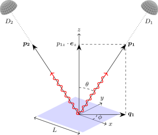
Figure 1: A sketch of the measurement scheme for investigating the two-photon signal. Both detectors are in the same vertical plane (at angle $\phi$ in the scheme). The semiconductor sample is pictured in blue, red wavy lines denote the emitted photons.

Each detector measures the number of photons emitted at a specific direction. To account for the background contribution, one may perform an additional ”out of plane” measurement with a slight shift of detector positions to violate the $\bm{q}_{1}=-\bm{q}_{2}$ condition and then subtract the results of the ”the same plane” measurement.

In order to subtract the background contribution in this manner, the detectors should be small and far enough to measure the far-field emission. This is essential for distinguishing a pure condensate (with macroscopic occupation of a single mode) from a quasicondensate (a bunch of low-lying states having macroscopically high occupations).

With fixed detector positions, the central quantity of our interest is the angled emission intensity from unit area in unit detector solid angle:

$$P(\theta,\phi)\equiv\dfrac{\Delta{P_{\rm angled}}}{\Delta{\Omega}}$$ (3)

and the corresponding two-photon decay time, given by

$$\tau_{2}(\theta,\phi)=\frac{n}{P(\theta,\phi)},$$ (4)

where $n$ is the exciton density.

III The microscopic model

The two-dimensional excitonic system is described by the following Hamiltonian:

$$\hat{H}\!=\!\sum\limits_{\bm{q}}T_{\bm{q}}\hat{Q}^{\dagger}_{\bm{q}}\hat{Q}_{\bm{q}}{+}\frac{1}{2L^{2}}\!\!\!\!\sum_{\bm{q},\bm{q}^{\prime},\Delta\bm{q}}\!\!\!U_{0}\left(\Delta\bm{q}\right)\hat{Q}_{\bm{q}}^{\dagger}\hat{Q}_{\bm{q}^{\prime}}^{\dagger}\hat{Q}_{\bm{q}^{\prime}{+}\Delta\bm{q}}\hat{Q}_{\bm{q}{-}\Delta\bm{q}},$$ (5)

where $\hat{Q}_{\bm{q}\lambda}$($\hat{Q}^{\dagger}_{\bm{q}\lambda}$) are the annihilation (creation) operators for excitons of momentum $\bm{q}$, $T_{\bm{q}}=E_{g}+q^{2}/2m_{\text{ex}}$ with $E_{g}$ and $m_{\rm ex}$ being the semiconductor exciton bandgap and the exciton mass respectively.

The operator $\hat{U}_{0}$ in (5) stands for exciton-exciton interaction. To deal with singular behavior of the potential we make use of a dressed interaction potential following Maximov et al. (2023b):

$$\begin{split}&\hat{U}=\hat{E}+\hat{U}_{1},\ \ \ \ \hat{E}=\int{e}_{0}(\hat{Q}^{\dagger}(\bm{r})\hat{Q}(\bm{r}))d\textbf{r},\\ \hat{U}_{1}=\dfrac{1}{2}\int&(U_{0}(\bm{r}{-}\bm{s}){-}g_{0}\delta(\bm{r}{-}\bm{s}))\hat{Q}^{\dagger}(\bm{r})\hat{Q}^{\dagger}(\bm{s})\hat{Q}(\bm{s})\hat{Q}(\bm{r})d\bm{r}d\bm{s}.\end{split}$$ (6)

Here we explicitly extracted the short-range contribution $g_{0}\delta(\bm{r}-\bm{s})$ out of the bare dipole-dipole interaction term $U_{0}(\bm{r})$ with $g_{0}={\int}U_{0}(\bm{r})d\bm{r}$ and replaced it by the short-range contribution with many-body effects taken into account in the local density approximation. Than, the remaining part is added in first Born approximation (see Appendix D) We use $e_{0}(n)$ for the free energy density component accounting for the many-body interactions, which is extracted from the results of an ab initio numerical simulation of the 2D system of dipoles at $T=0$Lozovik et al. (2007a). Thus, the dressed interaction is given by

$$U(\bm{r}-\bm{s})=U_{0}(\bm{r}-\bm{s})+\left[\frac{{\rm d}^{2}e_{0}(n)}{{\rm d}n^{2}}-g_{0}\right]\delta(\bm{r}-\bm{s}).$$ (7)

To model exciton recombination, we consider a bath of 3D photons:

$$\widehat{H}_{\text{3D}}=\sum\limits_{\bm{p}\lambda}\hbar\omega_{\bm{p}}\hat{c}_{\bm{p}\lambda}^{\dagger}\hat{c}_{\bm{p}\lambda},$$ (8)

with $\hat{c}_{\bm{p}\lambda}$ and $\hat{c}_{\bm{p}\lambda}^{\dagger}$ being the annihilation (creation) operators for a 3D photon with momentum $\bm{p}$ and polarization $\lambda$.

The exciton-photon coupling term is given as

$$\widehat{H}_{\rm int}={\sum\limits_{\bm{p},\lambda}}\bigg{(}L_{\bm{p}}^{\lambda}\widehat{Q}_{\bm{q}}\widehat{c}_{\bm{p}\lambda}^{+}+L_{\bm{p}}^{\lambda*}\widehat{Q}^{\dagger}_{\bm{q}}\widehat{c}_{\bm{p}\lambda}\bigg{)}.$$ (9)

Here $\bm{q}$ is the in-plane component of $\bm{p}$ in the same fashion as in Figure 1.

The coupling constant is expressed as follows Piermarocchi et al. (1996):

$$|L_{\bm{p}}^{\lambda}|^{2}=\dfrac{L^{2}}{V}\dfrac{\hbar^{2}c}{\tau_{\bm{p}}^{\lambda}\sqrt{\varepsilon}},$$ (10)

where $V$ is the quantization volume of the photonic bath, $\varepsilon$ is the dielectric constant of the environment and $\tau_{\bm{p}}^{\lambda}$ is the radiative exciton lifetime with respect to emission of a photon into the mode $\bm{p}\lambda$. Considering small $\bm{q}$, we omit the dependence of $\tau_{\bm{p}}^{\lambda}$ on polarisation and fix $p_{z}\approx E_{g}\sqrt{\varepsilon}/c\hbar$. Thus, the transverse momentum dependence is also further suppressed, $\tau_{\bm{p}}^{\lambda}\approx\tau_{r}$ Citrin (1993).

IV Two-photon emission intensity

Using the introduced microscopic Hamiltonian, one may express the desired two-photon signal in terms of the excitonic anomalous Green’s function ${F}_{\bm{q}}(t)=-i\braket{\mathcal{T}[\widehat{Q}_{\bm{q}}(t)\widehat{Q}_{-\bm{q}}(0)]}$ (see Appendix A for details):

$$P(\theta,\phi)=\bigg{(}\dfrac{p_{0}}{2\pi\hbar\tau_{\rm r}}\bigg{)}^{2}\dfrac{1}{\cos\theta}\int\limits_{-\infty}^{\infty}{dt}|F_{q_{0}}(t)|^{2}.$$ (11)

Here we took into account energy conservation which only allows photon emission with momentum $p_{0}=\mu\sqrt{\varepsilon}/c$ ($\mu\approx E_{g}$ is the condensate chemical potential). Its in-plane component magnitude is given by $q_{0}=p_{0}\sin(\theta)$. Remarkably, the anomalous Green’s function is nonzero only in the presence of a Bose condensate in the system. Thus, observation of the signal given by (11) unambiguously infers the presence of excitonic BEC.

In the scope of the standard BT, the anomalous Green’s function is given by the following expression (a decay term is introduced, see Appendix C):

$$\begin{split}iF(\bm{r},t)&=n_{0}-\frac{1}{L^{2}}\sum_{\bm{q}\neq 0}u_{\bm{q}}v_{\bm{q}}e^{i\bm{q}\bm{r}/\hbar}\times\\ &\times\bigg{(}(2n_{\bm{q}}+1)\cos\left(\dfrac{\varepsilon_{\bm{q}}t}{\hbar}\right)-i\sin\left(\dfrac{\varepsilon_{\bm{q}}|t|}{\hbar}\right)\bigg{)}e^{-|t|/2\tau_{\bm{q}}}\end{split}$$ (12)

with its Fourier image having the form

$$\begin{split}i&F_{\bm{q}}(t)=\int{e}^{-i\bm{q}\bm{r}/\hbar}iF(\bm{r},t)d\bm{r}=n_{0}\delta^{2}(\bm{q})-\\ &-u_{\bm{q}}v_{\bm{q}}\left[(1+2n_{\bm{q}})\cos\left(\frac{\varepsilon_{\bm{q}}t}{\hbar}\right)-i\sin\left(\frac{\varepsilon_{\bm{q}}t}{\hbar}\right)\right].\end{split}$$ (13)

The condensate density $n_{0}$ in the same framework is given as follows:

$$n_{0}=n-\frac{1}{L^{2}}\sum_{\bm{q}\neq 0}n_{\bm{q}}-\frac{1}{L^{2}}\sum_{\bm{q}\neq 0}v_{\bm{q}}^{2}\left(1+2n_{\bm{q}}\right).$$ (14)

Here $n_{Q}=n-L^{-2}\sum_{\bm{p}\neq 0}n_{\bm{p}}$ is the quasicondensate density, which insignificantly differs from the total density for excitonic systems under consideration, thus we neglect that difference further.

In the expressions above we used

$$u_{\bf q}=\frac{\varepsilon_{\bf q}+T_{\bf q}}{2\sqrt{\varepsilon_{\bf q}T_{\bf q}}},\ v_{\bf q}=\frac{\varepsilon_{\bf q}-T_{\bf q}}{2\sqrt{\varepsilon_{\bf q}T_{\bf q}}}$$ (15)

as the standard Bogoliubov coefficients, where $\varepsilon_{\bf q}=\sqrt{T_{\bf q}(T_{\bf q}+2n_{Q}U(\bf q))}$ is the excitation spectrum, $n_{\bm{q}}=1/(e^{\varepsilon_{\bm{q}}/T}-1)$ — excitation occupation number, $U(\bf q)$ is the Fourier transform of (7)).

With the help of the hydrodynamic approach along with the long-wavelength approximation, we derive a modified expression for the anomalous Green’s function and the condensate fraction (see Appendix C for an explanation of how the decay term is introduced in the first expression):

$$iF(\bm{r},t)=n_{0}\exp\bigg{\{}-\dfrac{1}{N}\sum\limits_{\bm{q}\neq{0}}u_{\bm{q}}v_{\bm{q}}e^{i\bm{q}\bm{r}/\hbar}$$ (16)

$${\times}\bigg{[}(2n_{\bm{q}}{+}1)\cos\left(\dfrac{\varepsilon_{\bm{q}}t}{\hbar}\right){-}i\sin\left(\!\dfrac{\varepsilon_{\bm{q}}|t|}{\hbar}\!\right)\bigg{]}e^{-|t|/2\tau_{\bm{q}}}\bigg{\}},$$

$$\frac{n_{0}}{n} =\exp\left(-\frac{1}{N}\sum_{\bm{q}\neq 0}v_{\bm{q}}^{2}\left(1+2n_{\bm{q}}\right)\right),$$ (17)

where $N$ is the number of particles in the system. We also introduced here $\tau_{\bm{q}}$ – the lifetime of excitation with momentum $\bm{q}$ (not to be confused with previously introduced $\tau_{\rm r}$, which is the exciton radiative lifetime). We used here the same technique as the one utilized in Voronova et al. (2018) for the normal Green’s function, see also Kane and Kadanoff (1967).

Note that the terms of both the sums in (12) and (16) are infrared divergent as $1/q^{2}$. For large enough $q$, the divergent terms do not contribute to the Fourier transform in (13), which is, however, not the case for (16). To deal with the divergence we regularize the sum utilizing a Lorentzian cutoff function as follows (here we take into account that in BEC regime one has $\tau_{c}=\tau_{\bm{q}}\big{|}_{\bm{q}=0}$), where $\tau_{\rm c}$ is the exciton system lifetime):

$$\ln \left(\frac{n_{0}}{iF(\bm{r},t)}\right)=\frac{1}{N}\sum_{\bm{q}\neq 0}\frac{mT}{q^{2}}\frac{1}{1+\beta^{2}\frac{q^{2}L^{2}}{(2\pi\hbar)^{2}}}e^{-|t|/2\tau_{c}}+$$

$$+ \int\frac{d^{2}\bm{q}}{(2\pi\hbar)^{2}n}\left\{u_{\bm{q}}v_{\bm{q}}e^{i\bm{q}\bm{r}/\hbar}\bigg{[}(2n_{\bm{q}}+1)\cos\left(\dfrac{\varepsilon_{\bm{q}}t}{\hbar}\right)-i\sin\left(\dfrac{\varepsilon_{\bm{q}}|t|}{\hbar}\right)\bigg{]}e^{-|t|/2\tau_{\bm{q}}}-\frac{mT}{q^{2}}\frac{1}{1+\beta^{2}\frac{q^{2}L^{2}}{(2\pi\hbar)^{2}}}e^{-|t|/2\tau_{c}}\right\}$$ (18)

with small dimensionless $\beta$. The first term in 2D has logarithmic dependence on $\beta$:

$$\frac{1}{N}\sum_{\bm{q}\neq 0}\frac{mT}{q^{2}}\frac{1}{1{+}\varepsilon^{2}\frac{q^{2}L^{2}}{(2\pi\hbar)^{2}}}=\frac{\alpha}{2\pi}\sum_{\bm{n}\neq 0}\frac{1}{|\bm{n}|^{2}}\frac{1}{1{+}\beta^{2}|\bm{n}|^{2}}=\alpha\ln\left(\frac{C_{1}}{\beta}\right)$$ (19)

where $\bm{q}=2\pi\hbar\bm{n}/L$ is the quantised momentum with the sum being over all 2D vectors $\bm{n}$ with integer coordinates. The dimensionless $\alpha$ is defined as $\alpha=T/T_{0}$ with $T_{0}=2\pi\hbar^{2}n/m_{\rm ex}$ being the degeneracy temperature of ideal 2D Bose gas. The coefficient $C_{1}$ is a shape factor of the semiconductor sample. Namely, considering a square of size $L\times L$ with periodic boundary conditions being imposed, numerical calculation leads to $C_{1}\approx 1.511$.

Clearly, the second term above has a logarithmic contribution due to $1/q^{2}$ behaviour of the integrand at small momenta, which may be cancelled by a proper choice of $\beta$ and, consequently, a cutoff momentum $q_{c}=\frac{2\pi\hbar}{L\beta}$. The value of $q_{c}$ is of the order of the smallest of momenta $\hbar/r$, $\hbar/c_{s}t$ and $T/c_{s}$, after which one of the factors $e^{i\bm{q}\bm{r}/\hbar}$, $cos(\varepsilon_{\bm{q}}t/\hbar)$ and $n_{\bm{q}}$ (correspondingly) deviates from its low-momentum behaviour. For excitonic systems under consideration (namely, in GaAs quantum wells and TMDC bilayers), the smallest momentum scale is set by $\hbar/(c_{s}t)$ for system size $L$ in range $\approx\left[c_{s}\tau_{\bm{q}};c_{s}\tau_{c}\right]$. Thus, we denote $q_{c}=C_{0}\hbar/(c_{s}t)$. That is why

$$iF(\bm{r} ,t)=n_{0}\exp\Bigg{(}\alpha\ln\left(\frac{C_{0}C_{1}L}{2\pi c_{s}t}\right)e^{-|t|/2\tau_{c}}+$$

$$+\int\frac{d^{2}\bm{q}}{(2\pi\hbar)^{2}n}\left\{u_{\bm{q}}v_{\bm{q}}e^{i\bm{q}\bm{r}/\hbar}\bigg{[}(2n_{\bm{q}}+1)\cos\left(\dfrac{\varepsilon_{\bm{q}}t}{\hbar}\right)-i\sin\left(\dfrac{\varepsilon_{\bm{q}}|t|}{\hbar}\right)\bigg{]}e^{-|t|/2\tau_{\bm{q}}}-\frac{mT}{q^{2}}\frac{1}{1+\frac{q^{2}c_{s}^{2}t^{2}}{C_{0}^{2}\hbar^{2}}}e^{-|t|/2\tau_{c}}\right\}\Bigg{)}.$$ (20)

The exact value of $C_{0}$ is obtained by numerically integrating the second term in (IV) and fitting logarithmic asymptotic behavior for $\ln(q_{c})\to\pm\infty$, which results in $C_{0}\approx 0.59\pm 0.02$ (see Appendix B).

After choosing a proper cutoff momentum, the second term has no logarithmic contribution. In addition, note that $\alpha$ should be a small quantity not to approach the BKT transition point, which corresponds to $\alpha_{\rm crit}\approx 0.2$ (in Nelson and Kosterlitz (1977) $\alpha=0.25$, however, in Lozovik et al. (2007b) it is demonstrated that finite-size effects on the BKT crossover as well as vortices, reduce it). Thus, one may expand up to the first order in $\alpha$ and consider the Fourier transform:

$$iF_{\bm{q}\neq\bm{0}} (t){=}{-}\frac{n_{0}}{n}\left(\frac{2\pi c_{s}t}{C_{0}C_{1}L}\right)^{\alpha e^{-|t|/2\tau_{c}}}$$ (21)

$${\times}{u_{\bm{q}}v_{\bm{q}}\!\bigg{[}(2n_{\bm{q}}+1)\cos\!\left(\!\dfrac{\varepsilon_{\bm{q}}t}{\hbar}\!\right){-}i\sin\!\left(\!\dfrac{\varepsilon_{\bm{q}}|t|}{\hbar}\!\right)\bigg{]}e^{-{|t|}/{2\tau_{\bm{q}}}}}.$$

The regularizing term in the integrand of (IV) does not contribute to the $F_{\bm{q}}(t)$ for finite $\bm{q}\neq 0$ due to independence of $r$. The zeroth order term of exponent expansion is omitted for the same reason.

Compared to the BT result (12), this expression has a size-dependent factor, which properly describes vanishing long-range order in a uniform 2D system of infinite size.

V Discussion

V.1 Numerical calculations for excitons

With the anomalous Green’s function being evaluated, we have the following expression for the two-photon radiation intensity:

$$P(\theta,\phi) =\!\bigg{(}\dfrac{q_{0}}{2\pi\hbar\tau_{\rm r}}\bigg{)}^{2}\!\dfrac{1}{\cos\theta}\left(\dfrac{n_{0}}{n}\right)^{2}\dfrac{(n{U}(\bm{q}))^{2}}{\varepsilon_{\bm{q}}^{2}}\!\left(\dfrac{1}{2}+n_{\bm{q}}+n_{\bm{q}}^{2}\right)$$

$$\times\int\limits^{\infty}_{0}\left(\dfrac{2{\pi}c_{s}t}{C_{0}C_{1}L}\right)^{2\alpha\exp(-t/2\tau_{c})}e^{-t/\tau_{\bm{q}}}dt.$$ (22)

This is the main result of the current study. We evaluate numerically the condensate fraction $n_{0}/n$ and investigate the dependence of the emission intensity on the size of the system, detection angle, etc. For further investigations, one needs the form of the excitation decay time $\tau_{q}$ dependence on the momentum $\bm{q}$. We use a model expression as explained in Appendix E.

Two physical realisations are considered simultaneously: excitonic gas in a GaAs/AlGaAs/GaAs quantum well and a one in a TMDC bilayer such as MoS₂/hBN/MoS₂.

The GaAs electron-hole separation is considered to be $D=12$ nm wide with dielectric constant $\varepsilon=12.5$, $m_{\rm ex}=0.22$ (in terms of the free electron mass)High et al. (2012). We use exciton radiative decay time $\tau_{\rm r}=20$ ns and the system decay time $\tau_{\rm{c}}=50$ ns.

For the MoS₂/hBN/MoS₂ structure, we use $D=1$ nm as the distance between TMDC layers (single hBN layer is considered as a spacer), $\varepsilon=7$, $m=0.88$ Fogler et al. (2014). For this system $\tau_{\rm r}=2$ ns and $\tau_{\rm{c}}=5$ ns.

As one would expect, for increasing detection angle $\theta$ we observe a sharp decrease of emission intensity. That is to say, the two-photon decay time $\tau_{2}(\theta,\phi)$ increases, as depicted in Figure 2.

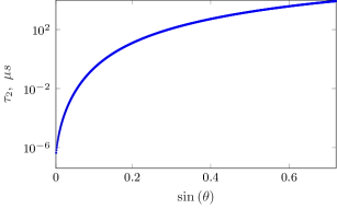
Figure 2: Angular dependence of two-photon decay time $\tau_{2}(\theta,\phi)$ for exciton gas in GaAs quantum well for $n=2\cdot 10^{10}$ cm^-2, $T=1$ K.

This graph does not demonstrate any qualitative deviation from the BT predictions, as well as no significant difference for TMDC excitons and quantum well excitons is revealed.

In contrast, we observe remarkable dependence on the system size for the two-photon decay time $\tau_{2}(\theta,\phi)$ (see Figure 3).

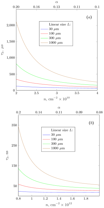
Figure 3: The two-photon decay time $\tau_{2}(\theta,\phi)$ as a function of particle surface density for (a) GaAs quantum well excitons at $T=1K$; (b) MoS₂ bilayer excitons at $T=10K$; for observation angle $\theta=\pi/6$

To reveal the deviations from the BT predictions, one may also consider the ratio (note that, for condensate fraction, we use (17) even for Bogoliubov expression since expression (12) becomes negative for the densities of interest):

$$\frac{P(\theta,\phi)}{P_{B}(\theta,\phi)}=\frac{1}{\tau_{\bm{q}}}\int\limits^{\infty}_{0}\left(\dfrac{2{\pi}c_{s}t}{C_{0}C_{1}L}\right)^{2\alpha\exp(-t/2\tau_{c})}e^{-t/\tau_{\bm{q}}}dt.$$ (23)

For $\tau_{\bm{q}}\ll\tau$, which appears to be the case for GaAs excitons observed at large enough angle $\theta$, the ratio scales as $L^{2\alpha}$, as demonstrated in Figure 3 (a). That is clearly exlained by replacing $\exp(-t/2\tau_{c})$ by unity in (23).

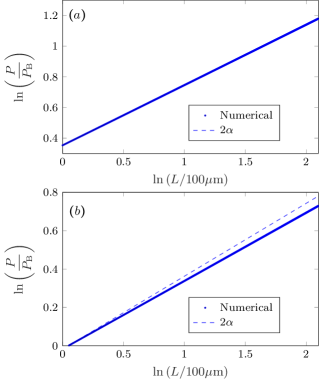
Figure 4: Dependence of the ratio $P/P_{B}$ on the sample linear size $L$ for (a) GaAs quantum well excitons of $n=2\cdot 10^{10}$ cm^-2; (b) TMDC monolayer excitons of $n=1\cdot 10^{12}$ cm^-2; for $\theta=\pi/6$. For both the plots $\alpha=0.19$.

For MoS₂ excitons, the ratio also scales approximately with the same exponent, as shown in Figure 4 (b).

V.2 Application to polaritonic condensates

The formalism we use in this study for excitonic systems is well-applicable for exciton-polaritons also, albeit with several modifications. Namely, instead of (24), one should use

$$\widehat{L}={\sum\limits_{\bm{p},\lambda}}\bigg{(}L_{\bm{p}}^{\lambda}\widehat{c}_{\bm{q}\lambda}\widehat{c}_{\bm{p}\lambda}^{+}+L_{\bm{p}}^{*\lambda}\widehat{c}^{\dagger}_{\bm{q}\lambda}\widehat{c}_{\bm{p}\lambda}\bigg{)}$$ (24)

where $\hat{P}_{\bm{q},\lambda}$ is the annihilation operator for a lower polariton, $\hat{c}_{\bm{q},\lambda}=(1-X^{2}_{\bm{q},\lambda})\hat{P}_{\bm{q},\lambda}$ stands for the annihilation operator of a two-dimensional photon in the absence of upper polaritons Grudinina et al. (2021) and $X^{2}_{\bm{q},\lambda}$ is the Hopfield coefficient.

In addition, one should replace the exciton lifetime $\tau_{\rm{r}}$ in the definition of $L_{\bm{p}}^{\lambda}$ by the polariton lifetime with respect to photon leakage out of the microcavity:

$$\tau_{\bm{q}}^{\rm pol}=\frac{1-X^{2}_{q}}{\tau_{\rm phot}}$$ (25)

with $\tau_{\rm phot}$ being the photon lifetime in the cavity. Clearly, one should also use the proper interaction potential when obtaining the condensate fraction.

However, we performed calculations for polaritons and observed only minor deviations from the BT results. This is due to small effective mass, which elevates the degeneracy temperature $T_{0}$, thus decreases $\alpha$, which makes the additional size scale factor negligibly different from zero. The only exception to consider is the case of extreme positive values of energy offset of the photonic spectrum with respect to excitonic one.

VI Conclusion

In this article we present an approach to calculating the two-photon emission intensity, which properly accounts for finite-size effects. It may be used to describe the results of HBT-type measurements for condensates of excitons and exciton-polaritons in both quantum wells and novel setups with 2D materials (e.g. TMDC layers).

By utilizing the hydrodynamic approach to the Bogoliubov theory, we considered the two-photon radiation intensity for a 2D Bose-condensate. Our results demonstrate that the standard Bogoliubov theory does not adequately predict the dependence of the radiation intensity on the size of the semiconductor sample. We claim that the modified expression we derive is the one that does.

VII Acknowledgements

I.L. Kurbakov acknowledges the support by the Russian Science Foundation grant No. 23-42-10010, https://rscf.ru/en/project/23-42-10010/ and the project FFUU-2024-0003. N.A. Asriyan acknowledges the support by the Russian Science Foundation grant No. 23-12-00115, https://rscf.ru/en/project/23-12-00115/.

Appendix A Emission intensity

We start from evaluating $P_{\rm total}$, introduced in Sec. II, thus we consider the density matrix evolution:

$$\rho(t)=\widehat{S}(t,-\infty)\rho_{0}\widehat{S}(-\infty,t)$$ (26)

with the $S$-matrix being given by a time-ordered exponent:

$$\widehat{S}_{t_{0}}(t_{2},t_{1}){=}\mathcal{T}\exp\bigg{(}{-}\dfrac{i}{\hbar}\int\limits_{t_{1}}^{t_{2}}(e^{{-}\delta|t|}\widehat{U}(t){+}\theta(t)\theta(t_{0}{-}t)\widehat{L}(t))dt\bigg{)}.$$ (27)

Here $\hat{U}$ and $\hat{H}_{\rm int}$ are expressed in the interaction representation with respect to the unperturbed Hamiltonian $\widehat{H}_{0}=\widehat{T}-\mu\widehat{N}+\widehat{H}_{3D}$ ($\hat{T}$ is the kinetic term). Namely,

$$\widehat{L}(t)={\sum\limits_{\bm{p},\lambda}}\bigg{(}L_{\bm{p}}^{\lambda}\widehat{Q}_{\bm{q}\lambda}(t)\widehat{c}_{\bm{p}\lambda}^{\dagger}(t)+h.c.\bigg{)}.$$ (28)

Here $\hat{c}_{\bm{p}\lambda}^{\dagger}(t)=e^{i\left[\omega_{\bm{p}}-\mu/\hbar\right]t}\widehat{c}_{\bm{p}\lambda}^{\dagger}$. As in the standard diagram technique, we consider adiabatic switching of the interaction term with $t_{0}\delta\ll 1$, while coupling to the 3D bath is present for the time of measurement only.

The unperturbed density matrix describes the exciton and photon subsystems separately:

$$\hat{\rho}_{0}\equiv\hat{\rho}(-\infty)=\hat{\rho}^{\text{exc}}{\times}\hat{\rho}^{\text{3D}}_{0}=\frac{e^{-(\widehat{T}-\mu\widehat{N})/T}}{\operatorname{Tr}\left[e^{-(\widehat{T}-\mu\widehat{N})/T}\right]}{\times}\ket{0}\!\bra{0}_{\text{3D}},$$ (29)

with $\ket{0}_{\rm 3D}$ being the photonic vacuum.

By decomposition of the S-matrix as a product $\widehat{S}_{t_{0}}=\mathcal{T}\widehat{S}_{U}\widehat{S}_{Lt_{0}}$ with

$$\widehat{S}_{U}(t_{2},t_{1})=\mathcal{T}\exp\left(-\dfrac{i}{\hbar}\int\limits_{t_{1}}^{t_{2}}\widehat{U}(t)e^{-\delta|t|}dt\right)$$ (30)

and

$$\widehat{S}_{Lt_{0}}=\mathcal{T}\exp\bigg{(}-\dfrac{i}{\hbar}\int\limits_{0}^{t_{0}}\widehat{L}(t)dt\bigg{)},$$ (31)

one may derive the following expression for the two-photon radiation intensity:

$$P_{\rm total}=\dfrac{1}{L^{2}t_{0}}\sum\limits_{\bm{p}\bm{p}^{\prime}}\braket{\widehat{S}_{Lt_{0}}^{U\dagger}\widehat{c}_{\bm{p}}^{\dagger}\widehat{c}_{\bm{p}^{\prime}}^{\dagger}\widehat{c}_{\bm{p}^{\prime}}\widehat{c}_{\bm{p}}\widehat{S}^{U}_{L\tau}}.$$ (32)

Here

$$\widehat{S}^{U}_{Lt_{0}}=\mathcal{T}\exp\bigg{(}-\dfrac{i}{\hbar}\int\limits_{0}^{t_{0}}\widehat{S}_{U}(0,t)\widehat{L}(t)\widehat{S}_{U}(t,0)dt\bigg{)}$$ (33)

is the interaction-renormalized $S$-matrix, the average in (32) is taken over the dressed density matrix

$$\rho_{H}\equiv\rho(0)=\widehat{S}_{U}(0,-\infty)\rho_{0}\widehat{S}_{U}(-\infty,0).$$ (34)

After expansion up to second order in $\widehat{L}$, we express the emission intensity

$$\begin{split}&P_{\rm total}{=}\dfrac{\braket{N_{1}N_{2}}}{L^{2}t_{0}}{=}\dfrac{1}{L^{2}t_{0}}\!\sum\limits_{\bm{p},\bm{p}^{\prime}}\!\dfrac{|L^{\lambda}_{\bm{p}}L^{\lambda}_{\bm{p}^{\prime}}|^{2}}{\hbar^{4}}\!\!\int\limits_{0}^{t_{0}}{d}t_{1}dt_{1}^{\prime}dt_{2}dt_{2}^{\prime}\\ &\times e^{-i(\hbar\omega_{\bm{p}}-\mu)(t_{1}-t_{2})/\hbar}e^{-i(\hbar\omega_{\bm{p}^{\prime}}-\mu)(t_{1}^{\prime}-t_{2}^{\prime})/\hbar}A,\end{split}$$ (35)

in terms of a Keldysh contour ordered product

$$A=\braket{\mathcal{T}_{C}[\widehat{Q}_{\bm{q}}^{U\dagger}(t_{1}^{\dagger})\widehat{Q}^{U\dagger}_{\bm{q}^{\prime}}(t^{\prime{+}}_{1})\widehat{Q}^{U}_{\bm{q}}(t_{2}^{-})\widehat{Q}^{U}_{\bm{q}^{\prime}}(t_{2}^{\prime{-}})]}.$$ (36)

The fact, that this is a time-ordered product on the Keldysh contour, is clear from the form of $\rho_{H}$ in (34). Symbols $\pm$ stand for the forward/backward branches.

Applying Wick’s theorem results in four terms (subscript _c stands for all connected diagrams):

$$A= \braket{\widehat{Q}^{U\dagger}_{\bm{q}}(t_{1})\widehat{Q}^{U}_{\bm{q}}(t_{2})}\braket{\widehat{Q}_{\bm{q}^{\prime}}^{U\dagger}(t_{1}^{\prime})\widehat{Q}^{U}_{\bm{q}^{\prime}}(t_{2}^{\prime})}+$$

$$\braket{\widetilde{\mathcal{T}}[\widehat{Q}^{U\dagger}_{\bm{q}}(t_{1})\widehat{Q}^{U\dagger}_{\bm{q}^{\prime}}(t_{1}^{\prime})]\mathcal{T}[\widehat{Q}^{U}_{\bm{q}}(t_{2})\widehat{Q}^{U}_{\bm{q}^{\prime}}(t_{2}^{\prime})]}_{c}+$$

$$\braket{\widehat{Q}^{U\dagger}_{\bm{q}}(t_{1})\widehat{Q}^{U}_{\bm{q}^{\prime}}(t_{2}^{\prime})}\braket{\widehat{Q}_{\bm{q}^{\prime}}^{U\dagger}(t_{1}^{\prime})\widehat{Q}^{U}_{\bm{q}}(t_{2})}+$$

$$\braket{\widetilde{\mathcal{T}}[\widehat{Q}^{U\dagger}_{\bm{q}}(t_{1})\widehat{Q}^{U\dagger}_{\bm{q}^{\prime}}(t_{1}^{\prime})]}\braket{\mathcal{T}[\widehat{Q}^{U}_{\bm{q}}(t_{2})\widehat{Q}^{U}_{\bm{q}^{\prime}}(t_{2}^{\prime})]}.$$ (37)

here we used $\widetilde{\mathcal{T}}$ as a antiordering operator. Operators with superscript ^U are defined in the same fashion as $\widehat{S}^{U}_{L\tau}$ in (33).

Of all the terms present here, only the fourth one has the desired sharp angularity as described in Section II due to a factor $\delta_{{\bm{q}},-{\bm{q}}}$. Indeed, the third term is proportional to $\delta(\bm{q},\bm{q}^{\prime})$, thus it vanishes for spatially separated detectors as depicted in Figure 1. The first and the second terms have smooth angular dependence (due to the assumption $\tau^{\lambda}_{\bm{p}}\approx\tau_{\rm r}$), thus, they contribute to background emission that is subtracted.

Substituting the fourth term from (A) into (35), we take the Fourier image of the anomalous Green’s function $F_{\bm{q}}(t)=-i\braket{\mathcal{T}[\widehat{Q}^{U}_{\bm{q}}(t)\widehat{Q}^{U}_{-\bm{q}}(0)]}$ and consider the integrals over times $t_{1},t_{1}^{\prime},t_{2},t_{2}^{\prime}$ :

$$P_{\rm angled}= \dfrac{1}{t_{0}S}\sum\limits_{\bm{p},\bm{p}^{\prime}}\dfrac{|L^{\lambda}_{\bm{p}}L^{\lambda}_{\bm{p}^{\prime}}|^{2}}{\hbar^{4}}\bigg{|}\int\limits_{-\infty}^{\infty}\dfrac{d\omega}{2\pi}F_{\bm{q}}(\omega)\int\limits_{0}^{t_{0}}dt\int\limits_{0}^{t_{0}}dt^{\prime}e^{i(\hbar\omega_{\bm{p}}{-}\mu{-}\hbar\omega)t/\hbar}e^{i(\hbar\omega_{\bm{p}^{\prime}}-\mu+\hbar\omega)t^{\prime}/\hbar}\bigg{|}^{2}=$$

$$= \dfrac{1}{t_{0}S}\sum\limits_{\bm{p},\bm{p}^{\prime}}\dfrac{|L^{\lambda}_{\bm{p}}L^{\lambda}_{\bm{p}^{\prime}}|^{2}}{\hbar^{4}}\bigg{|}\int\limits_{-\infty}^{\infty}\dfrac{d\omega}{2\pi}F_{\bm{q}}(\omega)e^{i(\hbar\omega_{\bm{p}}{-}\mu)t_{0}/2\hbar}2\pi\delta(\omega_{\bm{p}}{-}\mu/\hbar{-}\omega)e^{i(\hbar\omega_{\bm{p}^{\prime}}-\mu)t_{0}/2\hbar}t_{0}\rm{sinc}\left(\dfrac{(\hbar\omega_{\textbf{p}^{\prime}}{-}\mu{+}\hbar\omega)t_{0}}{2\hbar}\right)\bigg{|}^{2},$$ (38)

where $\bm{p}=\{\bm{q},p_{z}\}$, $\bm{p}^{\prime}=\{\bm{q},p_{z}^{\prime}\}$. Hereinafter, we assume that $t_{0}$ sets the largest timescale of the problem.

Integrating over frequency $\omega$, we obtain

$$P_{\rm angled}=\dfrac{1}{t_{0}S}\sum\limits_{\bm{p},\bm{p}^{\prime}}\dfrac{|L^{\lambda}_{\bm{p}}L^{\lambda}_{\bm{p}^{\prime}}|^{2}}{\hbar^{4}}|F_{\bm{q}}(\omega_{\bm{p}}-\mu/\hbar)|^{2}t_{0}{\rm sinc}\left(\dfrac{\hbar\omega_{\bm{p}}+\hbar\omega_{\bm{p}^{\prime}}-2\mu}{2\hbar}\right)2\pi\delta\left(\dfrac{\hbar\omega_{\bm{p}}+\hbar\omega_{\bm{p}^{\prime}}-2\mu}{\hbar}\right).$$ (39)

Given that $F_{\bm{q}}(\omega)$ decays rapidly at $\hbar\omega>mc_{s}^{2}(\sim 1\text{meV}$ in both GaAs and MoS₂), and $\mu\approx{E}_{g}\gg{m}c_{s}^{2}$, where $E_{g}$ is the semiconductor bandgap ($\sim{1}\text{eV}$ in both GaAs and MoS₂), in the sums over momenta $\bm{p}$ and $\bm{p}^{\prime}$ we can consider that $\omega_{\bm{p}}\approx\omega_{\bm{p}^{\prime}}\approx\mu/\hbar$.

Thus, going from the sum over $\bm{p}$ and $\bm{p}^{\prime}$ to the integrals, given $\delta_{\bm{q},-\bm{q}^{\prime}}$, using the substitution $\omega_{1,2}=c/(\hbar\sqrt{\varepsilon})\sqrt{q^{2}+p_{z1,2}^{2}}-\mu/\hbar$ ($p_{z1,2}>0$, the system is bounded from below by a mirror), considering $\omega_{1,2}\ll\mu$, we get

$$\begin{split}P_{\rm angled}=\int\dfrac{d^{2}\bm{q}}{(2\pi\hbar)^{2}}\dfrac{1}{2\pi\tau_{r}^{2}}\int{\dfrac{d\omega_{1}d\omega_{2}}{1-q^{2}/p_{0}^{2}}}|F_{\bm{q}}(\omega_{1})|^{2}\delta(\omega_{1}{+}\omega_{2}),\end{split}$$ (40)

where the expression for the matrix element (10) was substituted and $p_{0}=\mu\sqrt{\varepsilon}/c$. Integrating over $\omega_{2}$ with $d\bm{q}=p_{0}^{2}\cos\theta{d}\Omega$, we obtain the expression for the two-photon signal in angular variables:

$$\dfrac{\Delta{P}}{\Delta\Omega}=\left(\dfrac{p_{0}}{2\pi\hbar\tau_{r}}\right)^{2}\dfrac{1}{\cos\theta}\int\limits_{-\infty}^{+\infty}\dfrac{d\omega}{2\pi}|F_{{q_{0}}}(\omega)|^{2}.$$ (41)

Appendix B Anomalous Green’s function calculation

As described in the main text, the expression for the anomalous Green’s function (IV) has a contribution, which is logarithmically dependent on the system size. To properly extract it, we evaluate numerically the second term in the exponent, which is as follows:

$$I(q_{c})=\!\int\!\!\frac{d^{2}\bm{q}}{(2\pi\hbar)^{2}n}\left\{{-}\frac{mT}{q^{2}}\frac{1}{1{+}\frac{q^{2}}{q_{c}^{2}}}e^{{-}|t|/2\tau_{c}}\right.$$

$$\left.+u_{\bm{q}}v_{\bm{q}}e^{i\bm{q}\bm{r}/\hbar}\bigg{[}(2n_{\bm{q}}{+}1)\!\cos\!\left(\!\dfrac{\varepsilon_{\bm{q}}t}{\hbar}\!\right){-}i\!\sin\!\left(\!\dfrac{\varepsilon_{\bm{q}}|t|}{\hbar}\!\right)\bigg{]}e^{{-}|t|/2\tau_{\bm{q}}}\right\}=$$

$$=\alpha\ln\left(\frac{q^{*}_{c}}{q_{c}}\right)e^{-|t|/2\tau_{c}}+\Delta I(q_{c}),$$ (42)

for different values of $q_{c}$. Then, we fit asymptotic behavior of $I(q_{c})$ at $q_{c}\to\pm,\infty$, where logarithmic contribution is dominant with a function $f(q_{c})=\alpha\ln\left(q^{*}_{c}/q_{c}\right)\exp(-|t|/2\tau_{q})$. From the fitting, we derive the value of cutoff momentum $q_{c}^{*}$, which cancels the logarithmic contribution. This procedure is implemented for various values of $t$ for fixed $r$ and below we present the results in Figure 5, namely the fitted value $rq^{*}_{c}/\hbar$ as a function of $r/c_{s}t$.

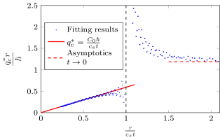
Figure 5: The dimensionless cutoff momentum $rq^{*}_{c}/\hbar$ as a function of the ratio $r/c_{s}t$. The linear part of the graph is utilized to derive the slope $C_{0}=0.59\pm 0.02$.

From the linear region of the graph, we derive the desired value of the slope $C_{0}=0.59\pm 0.02$.

Appendix C Introducing damping into the anomalous Green’s function

Considering the number of excitons $N$ to be finite and their decay to be weak ($\tau_{c}\gg L/c_{s}$, Wouters and Carusotto (2007)), one may neglect the difference between the superfluid $n_{s}$, the locally superfluid $n_{l}$, the quasi-condensate $n_{Q}$ (see Sec. IV) density and the total density $n$ in a sufficiently pure spatially homogeneous strongly correlated Lozovik et al. (2007a) exciton system at $\alpha\lesssim 0.2$. Thus, we apply the formalism developed in Voronova et al. (2018) for normal correlators to the calculation of the anomalous Green’s function:

$$iF({\bf r},t) =n\exp(-\langle\mathcal{T}[(\hat{\varphi}({\bf r},t)+\hat{\varphi}(0,0))^{2}/2]\rangle)=$$

$$=n_{0}\exp(-\langle\mathcal{T}[\hat{\varphi}({\bf r},t)\hat{\varphi}(0,0)]\rangle).$$ (43)

Here $n_{0}=n\exp\left(-\braket{\hat{\varphi}^{2}(0,0)}\right)$ is the density of the condensate (17) and

$$\hat{\varphi}({\bf r},t)=\frac{i}{\sqrt{N}}\sum_{{\bf q}\neq 0}\sqrt{\frac{\varepsilon_{\bf q}}{4T_{\bf q}}}(\hat{\alpha}_{\bf q}(t)-\hat{\alpha}^{+}_{\bf-q}(t))e^{i{\bf qr}/\hbar}$$ (44)

is the Heisenberg phase operator with $\hat{\alpha}_{\bf q}(t)$ being the bosonic excitation annihilation operator with momentum ${\bf q}$.

Substituting (44) into (C) and taking into account the absence of anomalous averages for the excitations, i.e. $\langle\hat{\alpha}_{\bf q}(t)\hat{\alpha}_{\bf q^{\prime}}(t^{\prime})\rangle=0$, we deduce

$$iF({\bf r},t) =n_{0}\exp\!\Big{[}-\!\sum_{{\bf q}\neq 0}\!\frac{e^{i{\bf qr}/\hbar}}{N}u_{\bf q}v_{\bf q}$$

$$\times\langle\mathcal{T}[\hat{\alpha}_{\bf q}(t)\hat{\alpha}^{+}_{\bf q}(0){+}\hat{\alpha}^{+}_{\bf q}(t)\hat{\alpha}_{\bf q}(0)]\rangle\!\Big{]}\!,$$ (45)

where we used $u_{\bf q}v_{\bf q}=n{U}(\bm{q})/2\varepsilon_{\bm{q}}$ (see (15)). We further substitute an ultraviolet cutoff factor $\varkappa_{\bf q}=1-T_{\bf q}^{2}/\varepsilon_{\bf q}^{2}$ in (C), following Voronova et al. (2018). This specific form ensures a proper unification of the quantum-field hydrodynamics with Bogoliubov’s theory for anomalous correlators.

The sum of time correlators in (C) in the inner brackets of the excitation operators can be expressed through their retarded $\mathcal{G}^{R}_{\bf q}(\omega)$ and the advanced $\mathcal{G}^{A}_{\bf q}(\omega)$ Green’s functions as

$$\langle{\mathcal{T}}[ \hat{\alpha}_{\bf q}(t)\hat{\alpha}^{+}_{\bf q}(0){+}\hat{\alpha}^{+}_{\bf q}(t)\hat{\alpha}_{\bf q}(0)]\rangle=$$ (46)

$$= \int_{-\infty}^{\infty}\frac{d\omega}{2\pi}[i\mathcal{G}_{\bf q}(\omega){+}i\mathcal{G}_{\bf q}(-\omega)]e^{-i\omega t},\vspace{-0mm}$$ (47)

where the causal excitation Green’s function is Abrikosov et al. (1963)

$$\mathcal{G}_{\bf q}(\omega)=(1+N(\omega))\mathcal{G}_{\bf q}^{R}(\omega)-N(\omega)\mathcal{G}_{\bf q}^{A}(\omega),\vspace{-2mm}$$ (48)

with $N(\omega)=1/(e^{\hbar\omega/T}-1)$.

In turn, the retarded (advanced) Green’s function is given by the analytic continuation of the Matsubara Green’s function $\mathcal{G}_{\bf q}^{M}(\omega_{s})$ to the upper (lower) half-plane Abrikosov et al. (1963)

$$\mathcal{G}_{\bf q}^{R(A)}(i\omega_{s})=\mathcal{G}_{\bf q}^{M}(\omega_{s}),\;\;\;\;\;\omega_{s}>0\;(<0).\vspace{-2mm}$$ (49)

Here $\omega_{s}=(2\pi T/\hbar)s$ is the Matsubara frequency and $s$ is an integer.

In a system with damping, the Matsubara Green’s function has the standard form Mahan (2000)

$$\mathcal{G}_{\bf q}^{M}(\omega_{s})=\frac{1}{i\omega_{s}-\varepsilon_{\bf q}/\hbar+i\rm{sign}(\omega_{s})/(2\tau_{\bf q})},\;\;\;\;\omega_{s}\neq 0.\vspace{-2mm}$$ (50)

Sequentially substituting (50) into (49), (49) into (48), (48) into (46), and the latter into (C), we obtain the final expression (16) for the anomalous Green’s function.

A similar calculation in the framework of the standard Bogoliubov theory is based on the expressions (48)-(50) and leads to (12).

Appendix D Dressed interaction

Here, we specify the form of ${U}({\bf q})$ (7) that is used in our calculations. We proceed in the same fashion as in our previous study Lozovik et al. (2017). Namely, as explained in the main text, the dressed coupling constant $g$ is extracted from the results of an ab initio simulation Lozovik et al. (2007a):

$$g\equiv U(0)=\frac{{\rm d}^{2}e_{0}(n)}{{\rm d}n^{2}}$$ (51)

with

$$e_{0}(n)\!=\!\frac{d^{2}}{\varepsilon r_{D}^{5}}a_{1}\exp[(1+a_{2})\ln u+a_{3}ln^{2}u+a_{4}ln^{3}u+a_{5}ln^{4}u].$$ (52)

Here $r_{D}=m_{\rm ex}d^{2}/\hbar^{2}\varepsilon$ and $u=nr_{D}^{2}$ is the dimensionless density, $d$ is the dipole moment of the exciton, $\varepsilon$ stands for the dielectric constant of the surrounding medium, and the analytical fit to the numerical simulation results is for $0.004\leq u\leq 8$ with coefficients being $a_{1}=9.218$, $a_{2}=1.35999$, $a_{3}=0.011225$, $a_{4}=-0.00036$, and $a_{5}=-0.0000281$.

We compose the dressed interaction of the dressed coupling constant $g$ and the bare remnant:

$$U(\bm{r})=g\delta(\bm{r})+\left[U_{0}(\bm{r})-\delta(\bm{r})\int{\rm d}^{2}\bm{r}U_{0}(\bm{r})\right].$$ (53)

For the latter we utilize the interaction potential for ”separated dipoles” , which is as follows:

$$U_{0}(r)=\frac{2e^{2}}{\varepsilon}\left(\frac{1}{r}-\frac{1}{\sqrt{r^{2}+D^{2}}}\right),$$ (54)

where $e$ is the elementary charge and $D=d/e$ is the electron-hole separation.

Appendix E Introducing the excitation lifetime

Calculating the excitation decay times for excitons is a complex problem due to multiple contributing decay channels: scattering on lattice phonons, free carriers, disorder potential, etc.

Not to deal with all these details, which do not affect the qualitative predictions of our study, we use the following model expression for the excitation decay rate:

$$\frac{\hbar}{\tau_{\bf q}}=\frac{\hbar}{\tau_{c}}+\Gamma_{\bf q},\;\;\;\;\Gamma_{\bf q}=\gamma_{0}T_{\bf q}\exp(-T_{\bf q}/gn).$$ (55)

Such a choice is motivated by the following simplistic considerations:

1. The damping $\hbar/\tau_{c}$ associated with the decay of the system is added to the $\Gamma_{\bf q}$ additively.

2. The contribution of $\Gamma_{\bf q}$ at small momenta is quadratic. Omission of the linear term is motivated by the fact that the thermal channel Popov (1983) contribution to the damping $\Gamma_{\bf q}$ is linearly dependent on $q$ and scales as a high power of $T$. The latter is low ($T\ll gn,T_{0}$), so this channel is weak.

   Other damping channels contribute with terms scaling as a power of momentum, which is higher than unity, e.g. the white-noise disorder contribution, as demonstrated in Giorgini et al. (1994).

3. For high momenta, $\Gamma_{\bf q}$ is a decreasing function.

In numerical calculations we use $\gamma_{0}=0.1$, which is to set the contribution of $\Gamma_{\bf q}$ to the order of a tenth of the value of the excitation spectrum itself for moderate momenta (one could choose any small value for which condensate still exists, this choice does not affect the results qualitatively).

References

- Byrnes et al. (2013) T. Byrnes, Y. Yamamoto, and P. van Loock, Phys. Rev. B 87, 201301 (2013), URL https://link.aps.org/doi/10.1103/PhysRevB.87.201301.
- J.Klaers et al. (2010) J.Klaers, J.Schmitt, F.Vewinger, and M.Weitz, Nature 468, 545 (2010).
- Maximov et al. (2023a) T. V. Maximov, I. V. Bondarev, I. L. Kurbakov, and Y. E. Lozovik (2023a), eprint 2304.02174, URL https://arxiv.org/abs/2304.02174.
- BROWN and TWISS (1956) R. H. BROWN and R. Q. TWISS, Nature 177, 27 (1956), ISSN 1476-4687, URL https://doi.org/10.1038/177027a0.
- Kasprzak et al. (2008) J. Kasprzak, M. Richard, A. Baas, B. Deveaud, R. André, J.-P. Poizat, and L. S. Dang, Phys. Rev. Lett. 100, 067402 (2008), URL https://link.aps.org/doi/10.1103/PhysRevLett.100.067402.
- Tempel et al. (2012) J.-S. Tempel, F. Veit, M. Aßmann, L. E. Kreilkamp, A. Rahimi-Iman, A. Löffler, S. Höfling, S. Reitzenstein, L. Worschech, A. Forchel, et al., Phys. Rev. B 85, 075318 (2012), URL https://link.aps.org/doi/10.1103/PhysRevB.85.075318.
- Gorbunov et al. (2009) A. V. Gorbunov, V. B. Timofeev, D. A. Demin, and A. A. Dremin, JETP Letters 90, 146 (2009), ISSN 1090-6487, URL https://doi.org/10.1134/S0021364009140148.
- Aßmann et al. (2010) M. Aßmann, F. Veit, J.-S. Tempel, T. Berstermann, H. Stolz, M. van der Poel, J. M. Hvam, and M. Bayer, Opt. Express 18, 20229 (2010), URL https://opg.optica.org/oe/abstract.cfm?URI=oe-18-19-20229.
- Takemura et al. (2012) N. Takemura, J. Omachi, and M. Kuwata-Gonokami, Phys. Rev. A 85, 053811 (2012), URL https://link.aps.org/doi/10.1103/PhysRevA.85.053811.
- Love et al. (2008) A. P. D. Love, D. N. Krizhanovskii, D. M. Whittaker, R. Bouchekioua, D. Sanvitto, S. A. Rizeiqi, R. Bradley, M. S. Skolnick, P. R. Eastham, R. André, et al., Phys. Rev. Lett. 101, 067404 (2008), URL https://link.aps.org/doi/10.1103/PhysRevLett.101.067404.
- Adiyatullin et al. (2015) A. F. Adiyatullin, M. D. Anderson, P. V. Busi, H. Abbaspour, R. André, M. T. Portella-Oberli, and B. Deveaud, Applied Physics Letters 107, 221107 (2015), ISSN 0003-6951, eprint https://pubs.aip.org/aip/apl/article-pdf/doi/10.1063/1.4936889/14471340/221107_1_online.pdf, URL https://doi.org/10.1063/1.4936889.
- Delteil et al. (2019) A. Delteil, C. T. Ngai, T. Fink, and A. İmamoğlu, Opt. Lett. 44, 3877 (2019), URL https://opg.optica.org/ol/abstract.cfm?URI=ol-44-15-3877.
- Perrin et al. (2012) A. Perrin, R. Bücker, S. Manz, T. Betz, C. Koller, T. Plisson, T. Schumm, and J. Schmiedmayer, Nature Physics 8, 195 (2012), ISSN 1745-2481, URL https://www.nature.com/articles/nphys2212.
- Hohenberg (1967) P. C. Hohenberg, Phys. Rev. 158, 383 (1967), URL https://link.aps.org/doi/10.1103/PhysRev.158.383.
- Mermin and Wagner (1966) N. D. Mermin and H. Wagner, Phys. Rev. Lett. 17, 1133 (1966), URL https://link.aps.org/doi/10.1103/PhysRevLett.17.1133.
- Lozovik et al. (2007a) Y. E. Lozovik, I. Kurbakov, G. Astrakharchik, J. Boronat, and M. Willander, Solid State Communications 144, 399 (2007a), ISSN 0038-1098, spontaneous coherence in exciton systems, URL https://www.sciencedirect.com/science/article/pii/S0038109807005790.
- Kane and Kadanoff (1967) J. W. Kane and L. P. Kadanoff, Physical Review 155, 80 (1967), URL https://link.aps.org/doi/10.1103/PhysRev.155.80.
- Voronova et al. (2018) N. S. Voronova, I. L. Kurbakov, and Y. E. Lozovik, Phys Rev Lett 121, 235702 (2018).
- Grudinina et al. (2021) A. M. Grudinina, I. L. Kurbakov, Y. E. Lozovik, and N. S. Voronova, Phys. Rev. B 104, 125301 (2021), URL https://link.aps.org/doi/10.1103/PhysRevB.104.125301.
- Brem et al. (2020) S. Brem, A. Ekman, D. Christiansen, F. Katsch, M. Selig, C. Robert, X. Marie, B. Urbaszek, A. Knorr, and E. Malic, Nano Letters 20, 2849 (2020), pMID: 32084315, eprint https://doi.org/10.1021/acs.nanolett.0c00633, URL https://doi.org/10.1021/acs.nanolett.0c00633.
- Brunetti et al. (2018) M. N. Brunetti, O. L. Berman, and R. Y. Kezerashvili, Journal of Physics: Condensed Matter 30, 225001 (2018), URL https://dx.doi.org/10.1088/1361-648X/aabe53.
- Wang et al. (2014) G. Wang, X. Marie, L. Bouet, M. Vidal, A. Balocchi, T. Amand, D. Lagarde, and B. Urbaszek, Applied Physics Letters 105, 182105 (2014), ISSN 0003-6951, eprint https://pubs.aip.org/aip/apl/article-pdf/doi/10.1063/1.4900945/14306079/182105_1_online.pdf, URL https://doi.org/10.1063/1.4900945.
- Tang et al. (2024) J. Tang, Y. Zheng, K. Jiang, Q. You, Z. Yin, Z. Xie, H. Li, C. Han, X. Zhang, and Y. Shi, Nano Research 17, 4555 (2024), ISSN 1998-0000, URL https://doi.org/10.1007/s12274-023-6325-3.
- Maximov et al. (2023b) T. V. Maximov, I. L. Kurbakov, N. S. Voronova, and Y. E. Lozovik, Phys. Rev. B 108, 195304 (2023b), URL https://link.aps.org/doi/10.1103/PhysRevB.108.195304.
- Piermarocchi et al. (1996) C. Piermarocchi, F. Tassone, V. Savona, A. Quattropani, and P. Schwendimann, Phys. Rev. B 53, 15834 (1996), URL https://link.aps.org/doi/10.1103/PhysRevB.53.15834.
- Citrin (1993) D. S. Citrin, Phys. Rev. B 47, 3832 (1993), URL https://link.aps.org/doi/10.1103/PhysRevB.47.3832.
- Nelson and Kosterlitz (1977) D. R. Nelson and J. M. Kosterlitz, Phys. Rev. Lett. 39, 1201 (1977), URL https://link.aps.org/doi/10.1103/PhysRevLett.39.1201.
- Lozovik et al. (2007b) Y. E. Lozovik, I. Kurbakov, and M. Willander, Physics Letters A 366, 487 (2007b), ISSN 0375-9601, URL https://www.sciencedirect.com/science/article/pii/S0375960107002812.
- High et al. (2012) A. A. High, J. R. Leonard, A. T. Hammack, M. M. Fogler, L. V. Butov, A. V. Kavokin, K. L. Campman, and A. C. Gossard, Nature 483, 584 (2012), ISSN 0028-0836, 1476-4687, URL https://www.nature.com/articles/nature10903.
- Fogler et al. (2014) M. M. Fogler, L. V. Butov, and K. S. Novoselov, Nature Communications 5, 4555 (2014), ISSN 2041-1723, URL https://www.nature.com/articles/ncomms5555.
- Wouters and Carusotto (2007) M. Wouters and I. Carusotto, Phys. Rev. Lett. 99 (2007).
- Abrikosov et al. (1963) A. Abrikosov, L. Gorkov, and I. Dzyaloshinski, Methods of Quantum Field Theory in Statistical Physics (Prentice-Hall, inc., Englewood Cliffs, New Jersey, 1963).
- Mahan (2000) G. D. Mahan, Many-particle physics, Physics of solids and liquids (Springer Science + Business Media, LLC, New York, 2000), 3rd ed., ISBN 978-1-4757-5714-9 978-1-4419-3339-3.
- Lozovik et al. (2017) Y. E. Lozovik, I. L. Kurbakov, and P. A. Volkov, Phys. Rev. B 95, 245430 (2017), URL https://link.aps.org/doi/10.1103/PhysRevB.95.245430.
- Popov (1983) V. N. Popov, Functional integrals in quantum field theory and statistical physics, no. v. 8 in Mathematical physics and applied mathematics (D. Reidel Pub. Co. ; Sold and distributed in the U.S.A. and Canada by Kluwer Academic Publishers, Dordrecht ; Boston : Hingham, MA, 1983), ISBN 9789027714718.
- Giorgini et al. (1994) S. Giorgini, L. Pitaevskii, and S. Stringari, Physical Review B 49, 12938 (1994), ISSN 0163-1829, 1095-3795, URL https://link.aps.org/doi/10.1103/PhysRevB.49.12938.