Actinide signatures in low electron fraction kilonova ejecta

Abstract

Neutron star (NS) mergers are known to produce heavy elements through rapid neutron capture (r-process) nucleosynthesis. Actinides are expected to be created solely by the r-process in the most neutron rich environments. Confirming if NS mergers provide the requisite conditions for actinide creation is therefore central to determining their origin in the Universe. Actinide signatures in kilonova (KN) spectra may yield an answer, provided adequate models are available in order to interpret observational data. In this study, we investigate actinide signatures in neutron rich merger ejecta. We use three ejecta models with different compositions and radioactive power, generated by nucleosynthesis calculations using the same initial electron fraction ($Y_{e}=0.15$) but with different nuclear physics inputs and thermodynamic expansion history. These are evolved from 10 - 100 days after merger using the sumo non-local thermodynamic equilibrium (NLTE) radiative transfer code. We highlight how uncertainties in nuclear properties, as well as choices in thermodynamic trajectory, may yield entirely different outputs for equal values of $Y_{e}$. We consider an actinide-free model and two actinide-rich models, and find that the emergent spectra and lightcurve evolution are significantly different depending on the amount of actinides present, and the overall decay properties of the models. We also present potential key actinide spectral signatures, of which doubly ionized ₈₉Ac and ₉₀Th may be particularly interesting as spectral indicators of actinide presence in KN ejecta.

1 Introduction

Compact object mergers involving at least one neutron star (NS), either with a second NS in a binary system (BNS) or with a black hole (BHNS), are broadly accepted to be sites of rapid neutron capture (r-process) nucleosynthesis (Lattimer & Schramm, 1974, 1976; Symbalisty & Schramm, 1982; Eichler et al., 1989; Rosswog et al., 1999; Freiburghaus et al., 1999), with observations of the kilonova (KN) AT2017gfo confirming that the electromagnetic (EM), radioactively powered counterparts to these events broadly follow theoretical predictions (e.g. Abbott et al., 2017; Cowperthwaite et al., 2017; Kasen et al., 2017; Smartt et al., 2017; Villar et al., 2017). AT2017gfo has been investigated in great detail, with both lightcurve (LC) (e.g. Tanaka et al., 2018; Wollaeger et al., 2018; Bulla et al., 2019; Kawaguchi et al., 2021) and spectral modelling indicating the presence of a broad range of r-process elements (e.g. Watson et al., 2019; Domoto et al., 2021; Gillanders et al., 2021; Domoto et al., 2022; Gillanders et al., 2022; Hotokezaka et al., 2023; Sneppen & Watson, 2023; Tarumi et al., 2023). Since AT2017gfo, two further KN candidates have been observed following the detection of long gamma-ray burst (lGRB) afterglows: GRB 211211A (Rastinejad et al., 2022) and GRB 230307A (Levan et al., 2024), though these lack the complete broadband observations of AT2017gfo, and only the latter has spectral data.

Through the study of NS mergers and subsequent KNe, the origin of r-process elements in the Universe may be investigated. Of particular interest is the creation of the heaviest known elements within the third r-process peak ($Z\geq 72$) and beyond to the actinides. These require extremely neutron rich conditions (electron fractions $Y_{e}\lesssim 0.2$) within the ejecta in order to be synthesised (e.g. Goriely et al., 2011; Korobkin et al., 2012; Wanajo et al., 2014; Wu et al., 2016; Nedora et al., 2021; Wu & Banerjee, 2022; Holmbeck et al., 2023). This criterion is broadly expected to be met in part of the dynamic ejecta of NS mergers, depending on the impact of weak interactions (e.g. Wanajo et al., 2014; Goriely et al., 2015; Fujibayashi et al., 2020; Nedora et al., 2021; Kullmann et al., 2022; Fujibayashi et al., 2023). Based on the nature of the central remnant, e.g. a promptly collapsed BH or short-lived (10s of ms) NS remnant, the requisite ejecta conditions may also be produced by accretion disc outflows (see e.g. Shibata & Hotokezaka, 2019; Wanajo et al., 2022; Kawaguchi et al., 2024). In order to fully determine the origin of actinides, and to answer the question of whether NS mergers are the sole astrophysical sites providing sufficiently neutron-rich conditions to create them, it is necessary to understand their observational signatures in KNe.

While observational data are relatively lacking, theoretical models predict a significant diversity in NS mergers and their associated KNe. Notably, LCs and emergent spectra are expected to vary depending on merger properties, such as component masses, spins, inclination to the observer. In addition, modelling depends on the nuclear equation of state (EoS), as well as diverse nuclear quantities related to the r-process nucleosynthesis occurring within the ejecta (e.g. Barnes et al., 2021; Zhu et al., 2021; Bulla, 2023; Kullmann et al., 2023; Sarin & Rosswog, 2024). The models produced for the analysis of KNe are therefore equally varied, with their intrinsic accuracy depending on the uncertainty in the aforementioned quantities, as well as the physics included in the modelling.

Of critical importance for KN modelling are the elemental composition and radioactive power of the merger ejecta, which arise from the initial r-process nucleosynthesis, and subsequent radioactive decay of unstable isotopes. As these decays power the KN, the details pertaining to specific interactions of various decay products within the ejecta directly affect the emergent LC and spectra, and thus have powerful diagnostic potential if properly understood. The radioactive power and composition are often related to the neutron abundance of the ejecta by the electron fraction $Y_{e}$, with lower values signifying a more neutron rich environment (see e.g. Cowan et al., 2021, for a review on r-process nucleosynthesis).

The parametrization of power and composition by $Y_{e}$ can be extended to calculations of expansion opacities, which are then used to constrain groups of elements present in KN ejecta following the evolution of broadband LCs (e.g. Kasen et al., 2017; Tanvir et al., 2017; Villar et al., 2017; Tanaka et al., 2020; Domoto et al., 2021, 2022). The identification of individual elements and species requires detailed spectral analysis (e.g. Watson et al., 2019; Domoto et al., 2021; Gillanders et al., 2021; Domoto et al., 2022; Gillanders et al., 2022; Sneppen & Watson, 2023; Tarumi et al., 2023). In both cases, models making use of atomic data (e.g. at least energy levels and radiative transitions), as well as ejecta compositions and power, typically from a general formula or taken from nuclear network outputs, are required in order to interpret observational data.

The case of low $Y_{e}$, actinide bearing ejecta is particularly challenging due to the large degree of uncertainty associated with such neutron rich conditions. From the nuclear perspective, many studies have shown that synthesised abundances of actinide species are poorly constrained due to unknown nuclear quantities such as nuclear masses, $\beta$-decay rates, decay channel branching ratios, and nuclear fission rates (e.g. Mendoza-Temis et al., 2015; Wu et al., 2019; Giuliani et al., 2020; Lemaître et al., 2021; Zhu et al., 2021; Wu & Banerjee, 2022). This leads to large variations in predicted abundances, as well as radioactive power, both of which are key ingredients in the modelling of KNe. Furthermore, the atomic structure of actinide species is typically poorly known, due to a lack of experimental atomic data, and the complexity of actinide species with partially filled, open f-shell configurations (e.g. Even et al., 2020; Tanaka et al., 2020; Flörs et al., 2023; Fontes et al., 2023).

In this work, we build on previous studies highlighting the observational impacts of uncertainties in the aforementioned quantities. We approach this issue from both a LC and spectral modelling perspective, making use of non-local thermodynamic equilibrium (NLTE) radiative transfer simulations in order to investigate potential actinide signatures from $\sim 10-100$ days after merger. We employ three models that have identical ejecta profiles and electron fractions of $Y_{e}=0.15$, but whose compositions and radioactive power are taken from different nuclear network calculations. The usage of NLTE radiative transfer simulations allows us to highlight potential actinide signatures in low $Y_{e}$ ejecta to late times in a self-consistent manner.

In Section 2 we present the models used in this study, as well as the radiative transfer simulation. We continue in Section 3 by presenting the temperature and ionization structure evolution of these models, highlighting the differences which lead to to spectral and LC variations as discussed in Section 4. Finally, we summarise our findings and present future directions in Section 5.

2 Models

We adopt three different models of nuclear composition and associated radioactive power from Barnes et al. (2016) and Wanajo et al. (2014). The calculations were computed using different thermodynamic trajectories and nuclear inputs, such as mass models and decay rates, but with the same electron fraction value of $Y_{e}=0.15$. The first two models, named ‘B16A’ and ‘B16B’, correspond to those computed using the same nuclear reaction network, employing different sets of nuclear ground-state masses from the Duflo-Zuker (DZ31 Duflo & Zuker, 1995) and the Finite Range Droplet Model (FRDM Möller et al., 1995) respectively. The underlying thermodynamic trajectory and all other nuclear reaction rates are the same for these two models. The third model named ‘W14’ used a different nuclear reaction network supplied with reaction rates that are all different from those used in the B16A/B inputs (see Wanajo et al., 2014; Barnes et al., 2016, for details pertaining to these calculations).

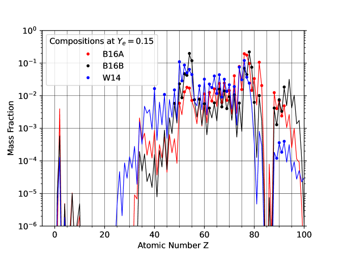
Figure 1: Compositions of the three models at 25 days (B16B, W14) and 27 days (B16A). Elements that are actively modelled in the radiative transfer simulation are marked by points (see text for explanation).

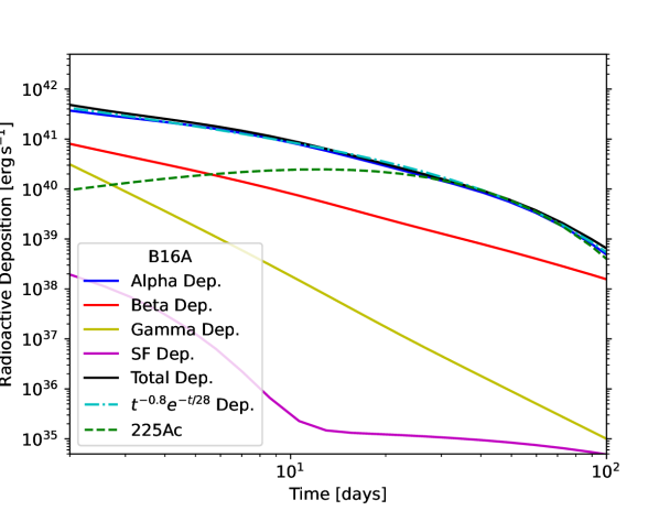
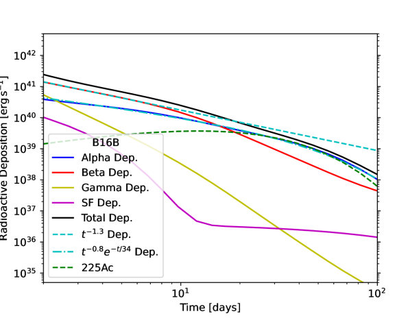
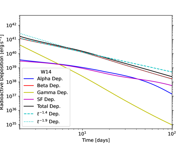
Figure 2: Energy depositions, including thermalization, by decay product for each model. Fits to the dominant sources of energy deposition in the models are shown in cyan. The green dashed line in the top and middle panels shows the deposition arising from the decay chain of ²²⁵Ac. Note that the simulation range is from 10 - 100 days.

Table 1: Model compositions by mass fractions. B16B and W14 are at 25 days, while B16A is at 27 days.

Element	B16A	B16B	W14
40Zr	-	-	0.0165
44Ru	-	-	0.0109
48Cd	-	0.0058	0.0151
50Sn	0.0059	0.0231	0.1101
51Sb	-	0.0087	0.0285
52Te	0.0131	0.0475	0.0871
53I	0.0181	0.0423	0.0502
54Xe	0.0171	0.1978	0.0642
55Cs	0.0072	0.1186	0.0445
56Ba	-	0.0075	-
58Ce	0.0079	0.0077	0.0201
60Nd	0.0113	0.0057	0.0321
62Sm	0.0126	0.0042	0.0228
63Eu	0.0069	-	0.0178
64Gd	0.0162	0.0060	0.0402
65Tb	-	-	0.0117
66Dy	0.0239	0.0159	0.0440
67Ho	0.0062	0.0045	0.0091
68Er	0.0244	0.0140	0.0319
69Tm	0.0072	0.0040	0.0135
70Yb	0.0144	0.0093	0.0216
72Hf	0.0408	0.0107	0.0190
74W	0.0785	0.0059	0.0753
75Re	0.0155	-	0.0310
76Os	0.1941	0.0700	0.1204
77Ir	0.1759	0.0445	0.0371
78Pt	0.0975	0.2205	0.0243
79Au	0.0146	0.0746	-
80Hg	0.0335	0.0062	-
82Pb	0.1060	0.0101	-
83Bi	0.0205	-	-
88Ra	0.0124	0.0042	-
89Ac	0.0040	0.0013	0.0001
90Th	0.0070	0.0075	0.0004
91Pa	0.0024	0.0033	0.0002
92U	0.0049	0.0185	0.0004

The ejecta models used in this study are all single-dimensional, composed of 5 radial velocity zones spanning $v_{\rm{ej}}=0.05c-0.30c$, increasing in steps of $0.05c$. The total ejecta mass is $M_{\rm{ej}}=0.05M_{\odot}$, and follows a density profile of $\rho\propto v^{-4}$. The models are all placed at 40 Mpc from the observer, similar to the distance inferred for AT2017gfo (e.g. Abbott et al., 2017). The compositions of each model are tabulated in Table 1. These compositions can be viewed graphically in Fig. 1, and the corresponding energy depositions in Fig. 2.

The compositions are limited to 30 elements, each with ion stages from neutral to triply ionized, due to memory constraints. The actinide species for which atomic data are available, ₈₉Ac - ₉₂U, are always selected, and the next 26 most abundant elements are then chosen. These abundances are taken at a fixed epoch for each model: 25 days for B16B and W14, and 27 days for B16A. This is done in order to avoid changing the model composition for each epoch, which would increase runtime and computational costs. The aforementioned epochs are chosen such that the composition reflects a rough average of the overall composition over the timespan of interest, $\sim 10-100$ days. From the nucleosynthesis calculations, we find that the maximal mass-fraction change in this time range occurs for ₈₉Ac in the B16A model, which has a fraction of $\sim 0.016$ at 11 days, $\sim 0.009$ at 109 days, and $\sim 0.012$ at our chosen epoch of 27 days. Note that these values are lower than those in Table 1, as they are relative to all elements from $\rm{Z}=1-105$, whereas the former are relative to the 30 chosen elements. While this does introduce a small level of inconsistency between the radioactive power and composition, the inaccuracy induced by this choice is believed to be far inferior to the intrinsic uncertainty from nuclear network inputs at this low $Y_{e}$, as well as the thermalization formulae used to calculate the final energy deposition (see below).

It should also be noted that the atomic mass of the elements is taken to be that of the most stable isotope, as the radiative transfer simulations do not distinguish between different isotopes of a given element. This will introduce some inconsistency in the number fractions derived from the mass fractions, as there will be variations in which isotopes are present at a given time, for a given species, due to the decay of unstable isotopes. However, as the models presented here are not sensitive enough to be greatly affected by the relatively small variations in number fractions introduced by this inconsistency, we expect the uncertainty arising from taking a constant atomic mass for each element to have a negligible impact on the emergent spectra.

From Figs. 1 and 2, the different outputs of the three models for an identical electron fraction are apparent. Considering first the B16B and B16A models which only differ by ground-state nuclear masses, we find significant variations in actinide production. Notably, the B16B model predicts peak actinide abundance for ₉₄Pu, as well as significant abundances of ₉₆Cm and ₉₈Cf, whereas the B16A values are markedly lower (red and black curves in Fig. 1). Unfortunately, atomic data for such heavy species are lacking, such that their spectral signatures cannot be modelled directly in the radiative transfer simulation. However, these species are important starting points for energetic spontaneous fission (SF) and $\alpha$-decay channels that may dominate power production should they be present in sufficient amounts (e.g. Barnes et al., 2016; Rosswog et al., 2017; Zhu et al., 2018; Wanajo, 2018; Wu et al., 2019; Giuliani et al., 2020; Holmbeck et al., 2023).

Indeed, looking at Fig. 2, we see that the B16A model has an energy deposition that is dominated by $\alpha$-decay across the entire 1 – 100 day timespan. There are several key differences between $\alpha$ and $\beta$-decay that must be taken into account in order to understand the impact on energy deposition. For similar lifetimes, $\alpha$-decays are typically stronger energy sources than $\beta$-decays, as they usually involve chains of several $\alpha$-decays (e.g. 4 for ²²⁵Ac) that produce $\alpha$-particles with kinetic energies significantly higher than $\beta$-decay electrons, $\sim 6$ MeV cf. $\sim 0.5$ MeV. From this, the raw radioactive power of $\alpha$-decay is greater than that of $\beta$-decay. The energy deposition is then further augmented by the efficient thermalization of $\alpha$-particles arising from their greater energy and higher charges (e.g. Barnes et al., 2016; Kasen & Barnes, 2019; Wu et al., 2019).

The $\alpha$-decay energy deposition in the two B16A/B models initially follows a power law, succeeded by an exponential decay. This is consistent with many nuclei undergoing $\alpha$-decay at early times and therefore yielding a power law relation, much like the canonical $t^{-1.4}$ power law for ensemble $\beta$-decay. At late times, we recover the specific decay chain of $\beta$-decay of ²²⁵Ra followed by $\alpha$-decay of ²²⁵Ac, as found previously in Wu et al. (2019). The B16B model has some additional late time contribution from the $\alpha$-decay of ²⁵³Es. The fact that the deposition follows the radioactive power so closely highlights how well $\alpha$-particles continue to thermalize in the bulk of the ejecta across the timespan considered here. It is also notable that the B16A model is much more energetic than the B16B model over the entirety of the 1 - 100 day range, which is expected to lead to brighter emergent luminosities.

In comparison to the B16A/B models, the W14 model produces a markedly different abundance pattern, particularly for the actinides. A very low actinide mass-fraction of $X_{\rm{Ac}}\sim 10^{-3}$ is yielded, approximately an order of magnitude less than the B16A and B16B calculations. Conversely, a higher lanthanide mass fraction is obtained ($X_{\rm{La}}\sim 0.26$ cf. $\sim 0.13$ for B16A), as well as significantly higher abundances of elements ranging from ₃₆Kr to ₅₀Sn, thus covering parts of the first and second r-process peaks.

The difference in heavy element production and their subsequent decay is also reflected in the energy deposition of this model, which is entirely dominated by $\beta$-decay, as shown in the bottom panel of Fig. 2. The early deposition follows the canonical $\dot{q}_{\rm{tot}}\sim t^{-1.4}$ power law, and drops to $\sim t^{-1.9}$ at later times. This contrasts with the predicted $t^{-2.8}$ post-thermalization break scaling (Kasen & Barnes, 2019; Waxman et al., 2019; Hotokezaka & Nakar, 2020). This is likely due to the layered nature of the ejecta, such that the inner layers are still thermalizing efficiently at late times, while the outer layers are not. This leads to an overall deposition that follows a power law steeper than the radioactive power generation at $t^{-1.4}$, but shallower than the complete post-thermalization break deposition at $t^{-2.8}$.

The W14 model also has a small spontaneous fission contribution at $\gtrsim 70$ days, which yet remains subdominant with respect to $\beta$-decay. A consequence of this, is that the W14 model has the lowest overall energy deposition for most of the epochs considered here, only becoming slightly more energetic than the B16B model at late times when the fission contribution comes in. The B16A model remains by far the most energetic over the whole period by a factor of $\sim 5$ more so than the other two models.

The above discussion highlights the importance of using time-dependent, radioactive energy deposition rates with consideration of the distribution of the various decay products as determined from network outputs, in order to fully capture the dependence on nuclear properties (e.g. Barnes et al., 2021). These effects are difficult to capture by analytical heating formulae despite the inclusion of multiple terms (e.g. Rosswog & Korobkin, 2022). In addition, the thermalization of decay products plays a fundamental role in the energy deposition, a subject which has been greatly studied (Barnes et al., 2016; Wollaeger et al., 2018; Kasen & Barnes, 2019; Waxman et al., 2019; Hotokezaka & Nakar, 2020; Zhu et al., 2021). In this work, the analytical thermalization equations from Kasen & Barnes (2019) are used for $\alpha$-decay particles, $\beta$-decay electrons/positrons, and $\gamma$-rays, with an additional input to the $\alpha$ and $\beta$-decay treatments from Waxman et al. (2019), while the prescription from Barnes et al. (2016) is employed for fission products, regardless of initial injection energy (see Appendix A of Pognan et al., 2023, for a detailed description of the employed formulae). While this treatment may not be the most advanced, the focus of this work is not the uncertainty present within thermalization physics, but rather the impact of uncertainties in the nuclear network inputs, i.e. the raw radioactive power, on potential actinide signatures in KNe. As such, an equal application of a relatively simple thermalization prescription is deemed to be satisfactory for the goals of this study.

2.1 Radiative transfer simulation

The radiative transfer simulations employ the spectral synthesis code sumo (Jerkstrand et al., 2011, 2012). sumo is a NLTE Monte Carlo code originally designed for nebular phase supernovae and adapted to model KNe, with the most recent updates for KN modelling described in Pognan et al. (2023). The three models are evolved over a timespan of $\sim 10-100$ days, in time-dependent NLTE mode (as initially described in Pognan et al., 2022a).

Compared to previous work, thermal collision strengths have been updated based on the work of Bromley et al. (2023), which found that the van Regemorter (van Regemorter, 1962, for allowed transitions) and Axelrod (Axelrod, 1980, for forbidden transitions) prescriptions systematically underestimate collision strengths for neutral to doubly ionized ₇₈Pt. Though this study was for a single r-process element, we take it as indicative of collision strength underestimation for all our r-process species, as other works for specific transitions have also found similar results (e.g. the Te iii 2.1$\mu$m line Madonna et al., 2018; Hotokezaka et al., 2023). In order to broadly correct for this effect, we apply a simple scaling factor to our calculations using the van Regemorter and Axelrod prescriptions, the exact value of which depends on ionization stage and temperature solution, but lying in the range of $1.5-10$ (see Appendix A for precise values). While this may lead to overestimation of collision strengths for certain transitions, it is impossible to quantify this effect, or even identify for which transitions this will occur until more atomic data for this process are available. Generally, increased collision strengths may lead to enhanced cooling as thermal collisions become more efficient.

Radiative transfer simulations of KNe must in general make use of atomic data, particularly atomic energy levels and transitions (wavelengths and A-values) in order to model the r-process species interacting in the ejecta. It is well known that the sparsity of atomic data for the majority of r-process species poses a particular challenge to KN modelling, which is found to be greater when addressing complex, line-rich species such as lanthanides and actinides (e.g. Even et al., 2020; Tanaka et al., 2020; Flörs et al., 2023; Fontes et al., 2023). Due to the lack of experimental atomic data, theoretical data sets calculated by atomic physics codes are often used.

The atomic data used in this study comes from calculations done using the Flexible Atomic Code (fac Gu, 2008, version from April 21st, 2021), and are identical to those used in Pognan et al. (2023), the purpose of which was completeness rather than detailed accuracy for key species. The configurations used for the fac calculations can be found in the appendix of Pognan et al. (2023), however the full configuration set for U iv was accidentally truncated. The ground state configuration remains [$\rm{5f^{3}}$], while the full list of additional configurations considered is [$\rm{5f^{2}\,6d^{1}}$,$\rm{5f^{2}\,7s^{1}}$,$\rm{5f^{2}\,7p^{1}}$,$\rm{5f^{1}\,6d^{2}}$,$\rm{5f^{1}\,6d^{1}\,7s^{1}}$,$\rm{5f^{1}\,6d^{1}\,7p^{1}}$]. More generally, it should be noted that the development of the methods implemented in fac has caused smaller variations in the resultant atomic data over the years from seemingly similar models. This should be considered when making detailed comparisons between data sets computed with different versions.

The NLTE radiative transfer simulations also make use of diverse cross-sections and rates (e.g. photoionization, recombination etc.) for the various processes included in the modelling. For r-process elements, data relating to these quantities are similarly lacking, such that fitting formulae or estimations are used instead. The details of the values used to model these diverse processes are described in Pognan et al. (2023), with only the aforementioned treatment of thermal collision strengths having been modified for this study.

3 Thermodynamic Evolution

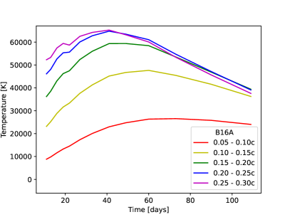
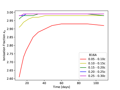
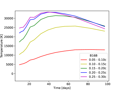
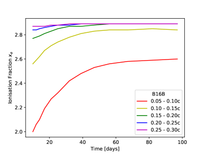
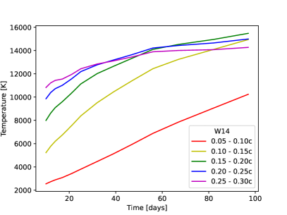
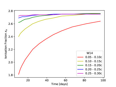
Figure 3: Temperature (left-hand panels) and ionization structure (right-hand panels) evolution of the three models, for each model zone. The ionization structure is characterized by electron fraction $x_{e}$, representing the number of free electrons per ion. Note that this is different from the compositional electron fraction $Y_{e}$.

We consider first the temperature and ionization structure evolution of the three models, which can be viewed in Fig. 3. Considering first the ionization structures shown in the right-hand panels, we see that all models exhibit remarkably similar evolution and structure, where the degree of ionization follows the overall energy deposition of the model, i.e. B16A is the most ionized, and W14 the least. A stratification is broadly found in every model, where the inner layers are typically less ionized than the outer layers, though some minor inversions do occur (e.g. in the W14 model at very late times). The low density in these outer layers inhibits both recombination and ionization processes, with recombination being more affected (see Pognan et al., 2023, for an analysis of ionization and recombination rates), thus usually leading to greater degrees of ionization.

In every model, the outermost three layers have an exceptionally flat ionization evolution, which is the result of time-dependent effects in the low density regime (Pognan et al., 2022a, 2023). In this regime, the efficiency of ionization and recombination is so low that a structure freeze-out is rapidly experienced, as the time-scales associated to these processes are comparable to, or even longer than the evolutionary time.

Considering now the temperature evolution, it is immediately noticeable that the B16A/B models are broadly similar, though the former is approximately twice as hot as a result of the greater energy deposition. Both models show an initially increasing temperature, which experiences a downturn and then begins to cool. The exact time at which this happens is density dependent, with the lower density, outer layers experiencing the downturn first around 40 days, while the innermost zone has a slower transition, around 60 days for B16A, and cooling has yet to fully begin in the innermost layer of the B16B model. It is also noteworthy that the slope of the temperature drop is greater for the outer layers, such that the outermost layer is no longer the hottest at 100 days. The slope of the outermost layer of the B16A model is also greater than that of the B16B model, which follows from enhanced line-cooling and adiabatic cooling at hotter temperatures.

In contrast, the W14 model follows more closely the evolution predicted by Hotokezaka et al. (2021); Pognan et al. (2022a), that is, a monotonically increasing temperature with time. It should be noted however, that the overall energy deposition does not follow the predicted post-thermalization break relation of $t^{-2.8}$, as explained in Section 2. As such, the exact temperature evolution for each zone does not necessarily follow the predicted $T\sim t^{0.2}$ relation (Hotokezaka et al., 2021), and it is clearly seen that the temperature for the innermost zone is still rising significantly faster than the outer zones which are inefficiently thermalizing $\beta$-decay electrons. The outermost layers of the W14 model also exhibit a temperature flattening due to time-dependent effects. Notably, adiabatic cooling plays a significant role at these late times, contributing a maximum of $\sim 30$ per cent to the overall cooling in the outermost layer.

The adiabatic cooling contribution is comparatively smaller for the B16A model, only reaching $\sim 11$ per cent, whereas it is much more significant in the B16B model at $\sim 47$ per cent. It should be noted however, that these values represent the contribution to total cooling; the adiabatic cooling in the B16A model is still physically greater than in the B16B model as the total cooling is greater, driven by hotter temperatures. Despite its notable contribution to the total cooling, adiabatic cooling is not the sole driving factor behind the temperature downturn. Indeed, the prediction of a monotonically increasing temperature assumes that $\beta$-decay dominates, and that the deposited energy from this decay follows a temporal evolution of $E_{\rm{dep}}\propto t^{-2.8}$ after the thermalization efficiency break. However, these two models are not $\beta$-decay dominated at these late times, but instead $\alpha$-decay dominated (see Fig. 2).

As described previously in Section 2, the late-time $\alpha$-decay energy comes mostly from the $\alpha$-decay of ²²⁵Ac, and follows more closely an exponential decay law given by the lifetime of ²²⁵Ra (21.5 days) that $\beta$-decays to ²²⁵Ac, as opposed to the ensemble decay power law seen for $\beta$-decay. Considering the heating rate per volume, we have (see equation (7) of Pognan et al., 2022a):

$$h(t)=M_{\rm{ej}}\dot{q}_{\rm{tot}}/\left(\frac{4\pi}{3}v_{\rm{ej}}^{3}t^{3}\right)\>\rm{erg\,s^{-1}\,cm^{-3}}$$ (1)

where $M_{\rm{ej}}$ is the ejecta mass (or zone mass for a given ejecta layer), $\dot{q}_{\rm{tot}}$ is the energy deposition including thermalization factor, $v_{\rm{ej}}$ the outer ejecta velocity (or outer zone velocity for a given ejecta layer), and $t$ is time. Assuming that $\alpha$-particles are thermalizing efficiently in bulk ejecta for the epochs of interest here, and therefore taking $\dot{q}_{\rm{tot}}\propto\rm{e}^{-t/\tau}$, we obtain a heating rate per volume scaling as $h(t)\propto t^{-3}\rm{e}^{-t/\tau}$. In the present case, we have $\tau\approx 21$ days, which is shorter than the evolutionary time-scales considered.

Conversely, the cooling rate per volume, which remains dominated by line cooling, is given by (see equation (13) of Pognan et al., 2022a):

$$c_{\rm{line}}(t)=\sum_{i}\Lambda^{i}(T,n_{e},n_{i})n_{e}n_{i}\>\rm{erg\,s^{-1}\,cm^{-3}}$$ (2)

where $\Lambda^{i}$ is the line cooling function for a given ion species, dependent on temperature $T$, ion density $n_{i}$ and electron density $n_{e}$, in complex and non-linear ways originating from the atomic structure of the species. Taking the line cooling function to be approximately independent of electron and ion density in low enough density regimes, such as those studied here, we find a cooling per volume of $c_{\rm{line}}(t)\propto t^{-6}$.

From the above equations, we find that the temporal evolution of the cooling at the late epochs studied here is shallower than that of the heating, once $\alpha$-decay following an exponential decay law dominates energy deposition. This is even more so when $\alpha$-decay thermalization begins to become inefficient, multiplying in a factor of $t^{-1.5}$ into the heating rate per volume, while cooling is further enhanced by adiabatic cooling scaling as $t^{-1}$ (see equation (8) of Pognan et al., 2023). Therefore, late-time cooling in $\alpha$-decay dominated regimes following an exponential decay law is expected, even without consideration of time-dependent effects such as adiabatic cooling.

The exact time at which the temperature downturn occurs however, will depend on the half-life, or half-lives, of the dominating $\alpha$-decay species. Notably, a shorter half-life will lead to an earlier temperature downturn, and vice-versa for a longer half-life. As such, the details of the transition from heating to cooling dominated regimes will depend on the outputs of the nuclear networks, notably the relative abundance of $\alpha$-decaying species with respect to each other.

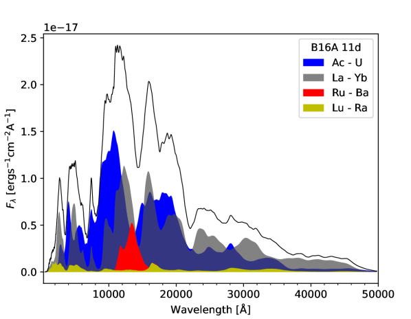
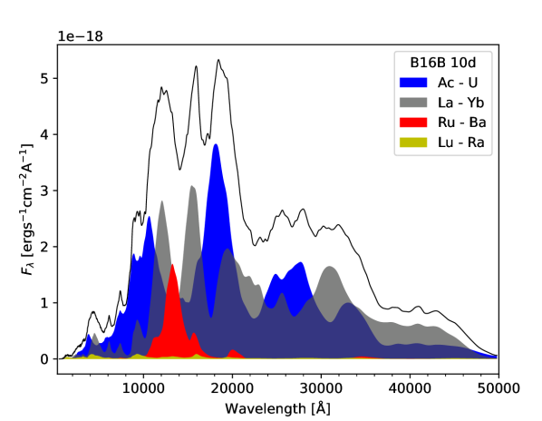
Figure 4: Contribution of element groups to the emergent spectra of the models at 11 days for B16A (top panel) and 10 days for B16B and W14 (middle and bottom panel respectively). Note the different flux levels, where the more energetic models are brighter.

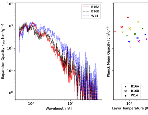
Figure 5: Expansion opacities averaged over zone mass for each model (left panel) and Planck mean opacities for each layer (right panel) at 11 days for B16A, and 10 days for B16B and W14. The color scheme of the markers in the right panel follows the same convention as in Fig. 3, i.e. red corresponds to the innermost layer and magenta to the outermost.

4 Spectra

4.1 Actinide-rich and actinide-free spectra

We first compare the emergent spectra of the actinide-rich B16A and B16B models, to the actinide-free spectrum of the W14 model at the earliest epochs studied here. The overall contributions of the various r-process element groups for each model spectra at $\sim 10$ days can be seen in Fig. 4. There is a striking lack of actinide features in the W14 model, arising from the small mass-fraction of these elements in the composition ($X_{\rm{Ac}}\sim 10^{-3}$, see Table 1). Instead, as the most lanthanide-rich model with $X_{\rm{La}}\sim 0.26$, the emergent spectrum is entirely dominated by lanthanide species, with this dominance remaining throughout all epochs studied here (see Appendix B). The W14 model also has a much lower emergent luminosity, following directly from the lower energy input (see Fig. 2).

It is interesting to find that even with relatively small actinide mass fractions of $X_{\rm{Ac}}\sim 0.018-0.030$ in the two B16A/B models, we recover significant actinide emission in the overall spectrum. As open f-shell species, actinides have a large energy level count and correspondingly numerous transitions. This allows them to efficiently absorb blue optical photons and produce redder photons through fluorescence cascades, even more effectively than the lanthanides (Flörs et al., 2023; Pognan et al., 2023). Several low lying transitions from actinide ions that are no longer open f-shell species, such as Ac iii and U iv described in the next subsection, also produce significant flux by direct emission, as opposed to fluorescence. These factors combined likely lead to the actinides providing anywhere from $\sim$ 40 – 80 per cent of the emergent model fluxes, despite their small mass fractions. There is naturally a limit however, and we see that the very low actinide mass fraction of $X_{\rm{Ac}}\sim 10^{-3}$ in the W14 model is insufficient to provide significant actinide emission in the emergent spectra.

The variations between the three models highlight the importance of a proper accounting of effects arising from choices of thermodynamic expansion history, as well as uncertainties in nuclear network inputs, on ejecta composition and emergent KN spectra. Notably, techniques making use of quantities such as expansion opacities and heating-rates parametrized by $Y_{e}$ in order to broadly infer ejecta properties are particularly susceptible. As is shown here, for a given $Y_{e}$, composition, radioactive power, and emergent spectra may be entirely different depending on which nuclear inputs are used, which for the low $Y_{e}$ ejecta considered here, are mostly based on theory as opposed to experimental measurement. This remains true when comparing models that have relatively similar total-heating rates, but distributed over different decay products, such as the B16B and W14 models in this case.

This impact is portrayed in Fig. 5, which shows the different expansion opacities and Planck mean opacities for the three models at the same epochs. These are found to be significantly distinct, following the aforementioned differences. Thus, expansion opacity calculations binned by $Y_{e}$ that are broadly used in radiative transfer simulations, or in the analysis of observations, must be well aware of the underlying nuclear physics being employed to yield the inputs to the opacity calculations, particularly when dealing with low $Y_{e}$ ejecta most susceptible to these uncertainties.

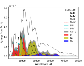
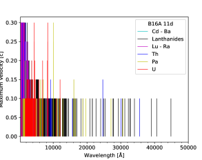
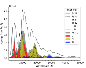
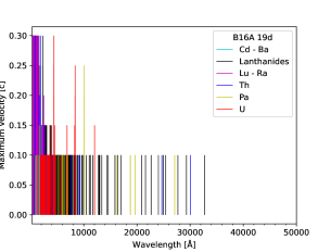
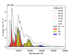
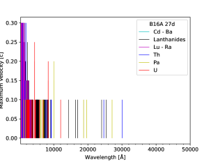
Figure 6: The B16A model spectra with actinide contributions marked out (left-hand panels) and corresponding optically thick lines ($\tau\geq 1$) at rest wavelength (right-hand panels), at 11, 19 and 27 days respectively.

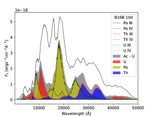
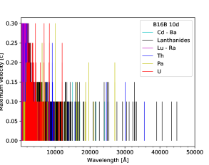
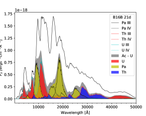
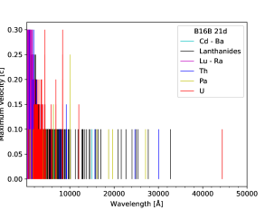
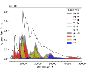
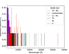
Figure 7: The B16B model spectra with actinide contributions marked out (left-hand panels) and corresponding optically thick lines ($\tau\geq 1$) at rest wavelength (right-hand panels), at 11, 21 and 32 days respectively.

4.2 Actinide contributions to the emergent spectra

The contribution of individual actinide species, as well as the optically thick lines present in the models, at selected epochs can be viewed in Figs. 6 to 9. Since the W14 model does not exhibit marked actinide features, we focus here on the B16A and B16B models, while the spectral evolution of the W14 model can be viewed in Appendix B.

Considering first Fig. 6, we have the B16A model spectra in the left-hand panels, and the corresponding optically thick lines in the right-hand panels, from 11 to 27 days. The optically thick line plots show optically thick ($\tau\geq 1$) transitions in the 5 model zones from velocity coordinates $v_{\rm{inner}}=0.05$c to $v_{\rm{outer}}=0.3$c, in steps of 0.05c. The height of the markers in the plot shows to which point in the ejecta the transition is optically thick e.g. if the marker reaches 0.2c, the transition is optically thick out until the third ejecta layer. In the analysis of the spectra below, we use the optically thick line plots to understand where absorption troughs in the spectra originate from.

Looking at the 11 days epoch in the top panels, the most active actinide species in spectral formation are found to be doubly and triply ionized ₉₁Pa and ₉₂U, with some weaker contributions from ₉₀Th. The main actinide-dominated features here are the ₉₂U P-Cygni like features at $\sim 4000$ and $\sim 8000\textup{\AA}$ respectively, and the blended ₉₁Pa and ₉₂U feature at 1 micron. The double feature from Pa iii and Pa iv at 1.7 micron contributes significantly to the emergent spectral shape at this wavelength, but does not entirely dominate, being heavily blended with lanthanide contributions (see Fig. 4). The U iv transitions, as well as the Pa iv transition at 1 micron, are found to be strong ($A\gtrsim 10^{5}\,\rm{s^{-1}}$) allowed transitions to the ground state. Conversely, the blended ₉₁Pa feature at 1.7 micron results from the contribution of many diverse allowed transitions with smaller radiative transition rates of $A\lesssim 10^{4}\,\rm{s^{-1}}$, typically seen in fluorescence cascades.

From the right-hand side of the top panels, we see that ₉₁Pa and ₉₂U have a few lines that are optically thick throughout the whole ejecta, and which line up with P-Cygni like features below 1 micron. We also note that the majority of the ejecta are optically thin beyond the innermost layer from about 1.8 micron and redwards, with the innermost layer only having a few optically thick lanthanide, ₉₀Th, and ₉₁Pa lines. At shorter wavelengths $\lambda\lesssim 6000\textup{\AA}$, we find a blend of many diverse optically thick lines, with important contributions from both the lanthanide species, as well as third r-process peak species.

Looking now at the middle and bottom panels of Fig. 6, we can see how the spectra and actinide signatures evolve with time in the B16A model. The spectral energy distribution (SED) follows the general evolution first seen in Pognan et al. (2023), with the spectra gradually becoming more blue with time. From the right-hand panels, we find that the ejecta begins to become entirely optically thin at redder wavelengths past $\sim 3$ micron, with the outermost layer also becoming optically thin below 1 micron down to 2000 Å. The aforementioned actinide-dominated spectral features evolve in relatively minor ways in this 10 - 30 day timespan, with red features generally fading more than the bluer features.

Fig. 7 shows the same plots as those described above, but for the B16B model. In the top panels, we see that the B16B model has actinide features dominated by the same species and ionization states as the B16A model, albeit with different relative contributions. For instance, more emission from Th iii at 2.8 and 3.4 micron features is found, which are low lying allowed E1 transitions with $\lambda_{0}=30096\,\textup{\AA}$, $\rm{A}\sim 10^{4}\,\rm{s^{-1}}$, and $\lambda_{0}=35551\,\textup{\AA}$, $\rm{A}\sim 10^{3}\,\rm{s^{-1}}$ respectively. In terms of optically thick lines, the B16A/B models are broadly similar, with the B16B model having somewhat more optical depth at redder wavelengths, and further out into the ejecta.

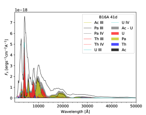
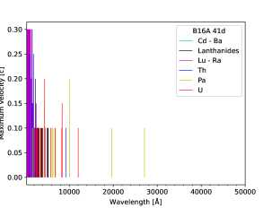
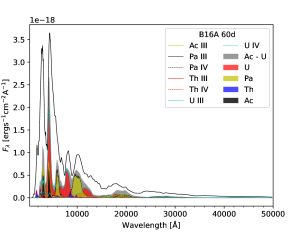
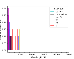
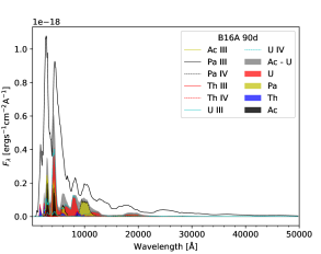
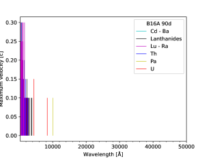
Figure 8: The B16A model spectra with actinide contributions marked out (left-hand panels) and corresponding optically thick lines ($\tau\geq 1$) at rest wavelength (right-hand panels), at 41, 60 and 90 days respectively.

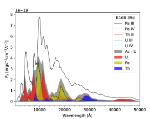
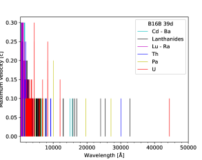
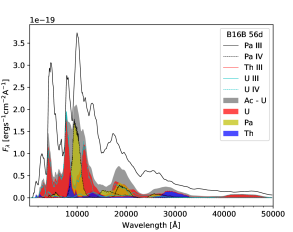
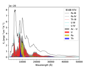
Figure 9: The B16B model spectra with actinide contributions marked out (right-hand panels) and corresponding optically thick lines ($\tau\geq 1$) at rest wavelength (left-hand panels), at 39, 56 and 97 days respectively.

Considering the evolution of the B16B model by looking at the middle and bottom panels of Fig. 7, we find that U iv begins to dominate the spectrum past 4 $\mu$m. The contribution of the Pa iii emission at 1.8 micron is greatly reduced with time, which is somewhat opposite of the behaviour seen in the B16A model, where the feature becomes dominant at that wavelength. Similarly to the B16A model, the B16B model becomes almost entirely optically thin past 3 micron, with a single optically thick U iv line in the innermost layer at 4.4 micron, the main contributor to U iv emission at that same wavelength. This transition is found to be an E1 dipole transition with a radiative transition rate of $A\sim 10^{3}\,\rm{s^{-1}}$.

The U iv emission at 4.4 micron in the B16B model, which dominates flux contribution there past $\sim 30$ days is somewhat reminiscent of the 4.5 micron Spitzer detection at 43 and 74 days for AT2017gfo (Kasliwal et al., 2022), which has been tentatively attributed to either Se iii or W iii by also taking into account the lack of detection at 3.6 micron (Hotokezaka et al., 2022). Looking at Table 1, we see that our models include ₇₄W, and in significant abundances for the B16A and W14 models. The relevant transitions of W iii for 4.5 micron emission are the $n=3\rightarrow 2$ and $n=2\rightarrow 1$ forbidden transitions with $\lambda=4.535\mu$m and $\lambda=4.432\mu$m respectively, following data available from the National Institute of Standards and Technology (NIST) Atomic Spectral Database (Kramida et al., 2020). The fac data for W iii have not been calibrated for this study however, and have these transitions at $\lambda=4.75\mu$m and $5.22\mu$m respectively. The former lies within the spectral range, and therefore may be expected to produce noticeable emission in the emergent spectra. Looking at the W14 model spectra in Appendix B, we see some W iii emission at $\sim 4.5$ micron appearing, though it remains largely subdominant compared to lanthanide emission at the same wavelength. In the B16A/B models however, no significant W iii emission is obtained.

This may be so for a variety of reasons. For forbidden transitions to be prominent, we require a significant abundance of the species, i.e. by elemental abundance and ion fraction, as well as the collisional de-excitation time-scale to be longer than the radiative transition lifetime, which is found to be on the order of $\sim 5$ s in our data. Considering first the B16A model at 41 days, we find that W iii is present mostly in the innermost ejecta layer with, but a relatively low ion fraction of $\sim 0.07$. Conversely, the B16B model at 47 days has a larger W iii ion fraction of $\sim 0.27$, but a much lower ₇₄W abundance in the model composition to begin with (see Table 1). As such, the W iii emission in both these models may be quite low in comparison to other species. It is also possible that the conditions for W iii forbidden emission are simply not met in the B16A/B models, requiring a balance between low density for inefficient collisions, but also a degree of ionization that favours W iii over W iv. Models with lower energy depositions than those yielded by dominant $\alpha$-decay, and therefore yielding significant ion fractions of W iii in low density ejecta, may be required in order for strong emission from this species to be produced.

Table 2: The U iv levels and associated transitions of interest in our model. The upper $\rm{5f^{2}6d^{1}}$ levels are compared to those in Seijo & Barandiarán (2003), while the lower $\rm{5f^{3}}$ levels to those from Carnall & Crosswhite (1985); Andres et al. (1996) (experimental measurements) and Ruipérez et al. (2007); Roy & Prasad (2020) (theoretical calculations).

Upper level ($\rm{5f^{2}\,6d^{1}}$)		Lower level ($\rm{5f^{3}}$)		Wavelength (Å)
$jj$-scheme $J^{\pi}_{n}$	$LS$ main componentsa	$jj$-scheme $J^{\pi}_{n}$	$LS$ main components b	FAC	Exp.c	Ab initiod
$(\nicefrac{{7}}{{2}})^{+}_{3}$	-	$(\nicefrac{{9}}{{2}})^{-}_{1}$	4I, 2H	4401	–	–
$(\nicefrac{{9}}{{2}})^{+}_{1}$	4I, 2H	$(\nicefrac{{9}}{{2}})^{-}_{1}$	4I, 2H	8366	3405	3405
$(\nicefrac{{5}}{{2}})^{+}_{1}$	4G, 2F	$(\nicefrac{{3}}{{2}})^{-}_{1}$	4F, 2D	44410	4295–4309	4407 - 6519

• Leading terms for $5f^{2}6d^{1}$ levels from Seijo & Barandiarán (2003).

• Leading terms for $5f^{3}$ levels from Roy & Prasad (2020).

• Experimental values from Carnall & Crosswhite (1985); Andres et al. (1996).

• Ab initio calculations from Ruipérez et al. (2007); Roy & Prasad (2020).

The later evolution of actinide features up to $\sim 90$ days are shown in Figs. 8 and 9 for the B16A and B16B models respectively. It is worth initially drawing attention to how slow the spectral evolution becomes at these late times. We note that the spectral shapes remain remarkably similar, aside from dropping flux levels and minor feature changes. The different model temperatures at these later epochs have a significant effect on the emergent spectra, as we see that the B16A model produces notably bluer features, with a smooth, featureless NIR continuum. In both models, we see that the entire ejecta becomes optically thin past 1 micron at later times, around 40 days for the B16A model, and closer to 60 days for the B16B model. Conversely, significant optical depth remains at the bluest wavelengths $\lambda\lesssim 4000$ Å in both models, for the entire duration of the timespan studied here.

The differences in emergent features between the B16A and B16B models are likely due more to the different temperature and ionization structure solutions, as opposed to differing abundances of actinide species. Notably, the B16B model is cooler and less ionized, such that features arising from doubly ionized species are typically stronger. Conversely, the B16A model has more important contributions from triply ionized species. This is well visualized by the relative Pa iii and Pa iv contributions to the emission at $\sim 1.8$ $\mu$m, where we see roughly equal contributions from these two species in the B16A model, but domination of Pa iii in the B16B model.

Of the various actinide features described above, some have a notable impact on the overall spectral shape, which may be detectable in observations. As described in Section 2, the atomic data underlying the emergent spectra come from theoretical calculations using the fac software, and are not calibrated to existing data, where such data exist. As such, it is important to verify whether the transitions giving rise to important spectral features are accurate and realistic when possible. Unfortunately, no existing literature data for the energy levels of Pa iii and Pa iv were found, and so we cannot verify the accuracy of the prominent ₉₁Pa features in our models.

The Th iii emission in our models may be checked by comparing our energy level structure to data available from NIST. In doing so, we find that the wavelengths of our prominent Th iii transitions are quite inaccurate, e.g. the emission at $\lambda_{0}=3.55\mu$m is in reality found to be at $13.0\mu$m, while the $\lambda_{0}=3.01\mu$m emission is at $22.3\mu$m. By also considering the change in radiative transition rate (A-value) arising from shifted energy levels, $A\propto\left(\Delta E_{\rm{NIST}}/\Delta E_{\rm{FAC}}\right)^{3}$ for dipole transitions (see e.g. Mulholland et al., 2024), we find A-values for the transitions at their correct wavelengths of $A_{13.0\mu m}\sim 1.7\times 10^{2}\,\rm{s^{-1}}$ and $A_{22.3\mu m}\sim 2.9\times 10^{1}\,\rm{s^{-1}}$ respectively. While this does mean that the Th iii emission in our model spectra cannot be taken directly as potentially observable actinide signatures, these results suggest that Th iii may produce significant mid-IR emission, should the temperature and ionization structure of the ejecta be comparable to those of the B16B model found here. The $22.3~{}\mu$m transition is particularly interesting, as it corresponds to the $n=3\rightarrow 2$ transition from the lowest lying $\rm{5f^{1}6d^{1}}$ state to the lowest lying $\rm{6d^{2}}$ state, and may therefore be a good candidate for late-time, nebular phase observations with JWST, given the relatively high A-value and low excitation energies of the involved levels.

At later times $\gtrsim 60$ days, the B16A model develops two Ac iii features at $\sim 3200,4400\textup{\AA}$ respectively, which blend with the U iii and U iv features, as well as emission from Tm iii and Eu iii, and Sm iii respectively. However, the $4400~{}\textup{\AA}$ emission from Ac iii provides approximately half of the actinide flux within the $\sim 5000\textup{\AA}$ emission feature. These Ac iii emission features are worthy of note, as the atomic data underlying them have wavelengths accurate to within 2 per cent, and A-values within a factor of 2, of data available from NIST. As such, these features are robust predictions that may remain important even if the other features in that area, of which the accuracy is difficult to verify, are corrected to other wavelengths or flux levels. However, it is difficult to predict whether they will become more or less dominant in that regime if the calibration of other atomic species yields a greater number of important transitions in the same wavelength range.

The verification of the features arising from U iv is more complicated, as no level data is readily available from NIST. The three features that are found to be significant in our model spectra arise from transitions between low-lying even parity $\rm{5f^{2}6d^{1}}$ states, to odd parity $\rm{5f^{3}}$ states. Several experimental measurements (Carnall & Crosswhite, 1985; Andres et al., 1996) and Ab initio theoretical calculations (Ruipérez et al., 2007; Roy & Prasad, 2020) of low-lying $\rm{5f^{3}}$ levels in U iv are available, while only a single theoretical calculation for $\rm{5f^{2}6d^{1}}$ levels was found (Seijo & Barandiarán, 2003).

One caveat of matching energy levels across different works is that it is often difficult to identify exactly which level corresponds to which due to differences in term labelling. The LSJ term notation is more commonly used in databases and in literature, particularly for low-energy structures which are easier to compute (Kramida et al., 2020). While fac, like other relativistic atomic codes, proceeds with calculations under a jj-coupling scheme, contrary to other codes fac uniquely lacks an internal mechanism for converting to LSJ notation. To address this, we employ the jj2lsj module (Gaigalas et al., 2017) from the grasp2018 software package (Froese Fischer et al., 2019). This module transforms atomic state functions from a jj-coupled configuration state function (CSF) basis to an LSJ-coupled CSF basis.

We use this program to extract LS leading terms from our theoretical data, and find the closest matching levels from literature. Of relevance to the transitions of interest in our model, our calculations show leading terms ${}^{4}\text{I}$ and ${}^{4}\text{F}$ for levels $(\nicefrac{{9}}{{2}})^{-}_{1}$ and $(\nicefrac{{3}}{{2}})^{-}_{1}$ respectively, associated with the odd $\rm{5f^{3}}$ configuration, and ${}^{2}\text{G}$, ${}^{4}\text{G}$ and ${}^{4}\text{I}$ for levels $(\nicefrac{{7}}{{2}})^{+}_{3}$, $(\nicefrac{{5}}{{2}})^{+}_{1}$, and $(\nicefrac{{9}}{{2}})^{+}_{1}$, associated with the even $\rm{5f^{2}\,6d^{1}}$ configuration. For most levels of interest, the labels we find seem to be reliable, with the contribution of the leading CSF being greater than 64 per cent, except for level $(\nicefrac{{7}}{{2}})^{+}_{3}$ where we see high mixing with first and second components of the wave-function, with contributions of 20 per cent (term ${}^{2}\text{G}$) and 18 per cent (term ${}^{2}\text{F}$) respectively. The wavelengths of our key transitions compared to those found using the energy levels in literature are shown in Table 2.

From this analysis, we see that the U iv feature at 4401 Å cannot be verified as no clear matching upper level is found in literature. For the other two transitions, energy levels in literature predict much bluer wavelengths than those found in the fac data. By following the dipole transition A-value scaling as described above, we also find that the radiative transition rates of the transitions initially at 8366 and 44410 Å will be greatly enhanced, which suggests that U iv should be playing a larger role in the absorption of blue photons in our model. Experimental measurements of the absorption spectra of U iv for $\rm{5f^{3}}$ to $\rm{5f^{2}6d^{1}}$ transitions have also found significant transitions in wavelengths ranging from 2500 – 6700 Å (Karbowiak, 2005). This implies that the main impact of U iv on KN spectra may actually be strong suppression of blue photons, with potentially enhanced fluorescence to redder wavelengths.

In general, the above analysis highlights the difficulty of robustly establishing spectral actinide signatures due to the sparsity of accurate available data. Comparison to such data when possible reveals that Ab initio calculations from theoretical atomic physics codes that focus on completeness rather than accuracy, as is the case for the fac dataset used here, may lead to highly inaccurate transition wavelengths. This effect is particularly important for IR transitions, where very slight deviations in energy level structure leads to large variations in transition wavelength. However, even literature values may find significantly different energy level values depending on the calculation (see e.g. Ruipérez et al., 2007; Roy & Prasad, 2020, for the $\rm{5f^{3}}$ levels of U iv). In order to provide better constraints on the spectral signatures of actinides in KN ejecta, higher accuracy atomic data is required, whether by experimental measurement or more detailed, targeted Ab initio theoretical calculations.

4.3 Broadband lightcurves

In general, the B16A and B16B models predict several key actinide features that produce significant impacts on the emergent spectra. As previously noted however, the accuracy of these features is for the most part difficult to verify, with the exception of the late time Ac iii emission. Therefore, a complementary approach to the identification of actinide signatures in KNe may be taken by studying the broadband LCs of the models, which are less susceptible to the exact wavelengths of key features, and generally more representative of the overall SED shape and evolution.

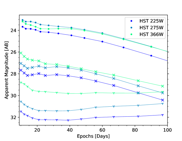
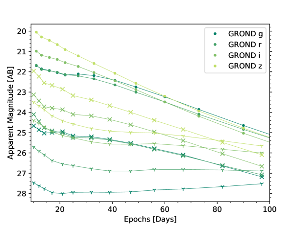
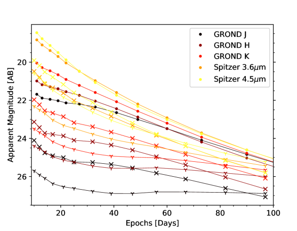
Figure 10: Broadband lightcurves of the models in the UV (top panel), optical (middle panel) and IR (bottom panel). The points correspond to the B16A model, the crosses to the B16B model, and the ‘Y’-shaped markers to the W14 model.

We conduct synthetic photometry on the emergent spectral series from near UV wavelengths to the MIR, the results of which are shown in Fig. 10. The top panel shows the near UV bands, for which we have used the Hubble Space Telescope (HST) wide-field camera’s F225W, F275W and F336W filters. The middle panel shows optical bands, where we have used the g,r,i,z bands of the Gamma-Ray Burst Optical/Near-Infrared Detector (GROND) instrument, mounted on the MPI/ESO 2.2m telescope at La Silla in Chile. Finally, the bottom panel shows IR bands, where the NIR is covered using the GROND instrument’s J,H,K bands, and we also include the 3.6 and 4.5$\mu$m bands from the Infra-Red Array Camera (IRAC) instrument on the Spitzer space telescope.

These choices are motivated by the spectral range of our radiative transfer simulations, which have been set to 5 micron in order to include the 3.6 and 4.5 micron bands of IRAC, of relevance to late time observations of AT2017gfo (Kasliwal et al., 2022). While many facilities observed AT2017gfo across other wavelengths, we have chosen the HST for the UV, and GROND for the optical/NIR in order to minimize the number of different instruments considered.

Analysing first the overall trends in each waveband, we find that the actinide-free model of W14 evolves qualitatively differently to the actinide-rich models. This model shows an initial decline in every waveband, followed by a relatively flat evolution, or even a slight increase in apparent magnitude for optical and UV wavebands. This is most noticeable for bluer wavebands, and corresponds to the spectra becoming progressively bluer with time due to rising temperatures and decreasing optical depths in homogeneous composition models (Pognan et al., 2023). The two Spitzer MIR bands however, show a continuous decrease in magnitude.

In contrast, the actinide-rich B16A and B16B models show a relatively different evolution. After an initial decrease, the UV and bluer optical bands tend to show a slight bump, or at least a plateau, between 20 - 40 days. Following this, a steady decrease in magnitude is found across all wavebands, the exact rate varying from band to band. This bump or plateau found in some of the broadband LCs of the actinide-rich models likely arises from flux moving bluewards as time progresses. However, in contrast to the W14 model which prolongs this plateau, or even yields a brightening in bluer wavebands, the actinide-rich models fade in every waveband past the $\sim 40$ day mark.

In both the B16A and B16B cases, this rate of decline is greater than that of the W14 model, such that the latter appears brighter than the B16B model in certain wavebands at the end of the timespan studied here (e.g. z-band from 80 days onwards). The B16A model typically remains brighter in every waveband however, likely due to the overall greater power output of the nuclear network. The generally hotter temperatures from greater radioactive power of the actinide-rich models leads them to be comparatively more blue than the W14 model. This effect is somewhat opposite of that expected by consideration of expansion opacities (e.g. Flörs et al., 2023; Fontes et al., 2023), however it is not fully clear how the red-to-blue evolution will present itself in cases of inhomogeneous composition, 3D models. As such, we present this comparison fully in the context of the models studied here.

The key differences in the evolution of the broadband LCs between the actinide-rich and free models is likely linked not only to the different model compositions, but also to the different temperature evolutions. Looking at Fig. 3, we see that the actinide-rich models start to cool around 40 - 60 days, whereas the W14 model continues to become hotter with time. The combination of this temperature increase with the dropping optical depth at bluer wavelengths allows the actinide-free model to efficiently transfer flux bluewards. In the actinide-rich models however, the dropping temperatures work against this process, such that it is less efficient. This factor, combined with the overall decreasing luminosity as nuclear energy input drops, leads to the steady fading of the B16A/B models across every waveband.

These results indicate that actinide-rich and actinide-free models may be distinguished by the evolving shape of their broadband LCs, not only arising from different compositions, but perhaps mainly from different resultant nuclear power and therefore corresponding temperature evolution.

5 Discussion and Conclusion

In this study, we have confirmed that uncertainties in nuclear physics inputs, such as mass models and nuclear decay rates, as well as choice of thermodynamic expansion history for nucleosynthesis, play important roles in the final composition and radioactive power of KNe, as has been shown in diverse prior studies (e.g. Barnes et al., 2021; Zhu et al., 2021; Kullmann et al., 2023). Using trajectories with $Y_{e}=0.15$ obtained from merger simulations, and based on the radioactive power and decay products predicted by full nuclear network calculations, we have evolved three different models over a timespan of 10–100 days, producing spectra and LCs using the sumo NLTE radiative transfer code.

From the emergent spectra and LCs, we find markedly different evolutions between the two actinide-rich B16A/B models, and the actinide-free W14 model. We find that the difference in radioactive power between these models leads to significantly distinct temperature and ionization structures, which drive dissimilar emergent spectral series. This effect, alongside important differences in composition, lead to noticeably different observable signatures both from a spectral and LC perspective.

The actinide-rich models evolve differently in the NLTE regime than predicted by previous results (Hotokezaka & Nakar, 2020; Hotokezaka et al., 2021; Pognan et al., 2022a), notably undergoing a temperature downturn in the 40 - 60 day range. This originates from the dominance of $\alpha$-decay following an exponential decay law over ensemble $\beta$-decay following a $t^{-2.8}$ power law in the energy deposition. The late time cooling plays a major role in the overall evolution of these models, driving the aforementioned differences between them, and the actinide-free W14 model. Furthermore, the B16A/B models suggest actinide signatures that may be detectable in an emergent spectrum, despite the presence of other line-rich species such as lanthanides. In both cases, the actinide mass fraction remains relatively small ($X_{\rm{Ac}}\sim 0.02-0.03$) in comparison to the lanthanide fraction ($X_{\rm{La}}\sim$ 0.12).

We provide a first attempt at constraining possible actinide signatures in KN spectra across a broad range of time-scales and wavelengths. We find that our actinide atomic data as calculated by fac targeting completeness over accuracy, yields transitions that are for the most part highly inaccurate, or unverifiable due to lack of reference data in the literature. The exceptions to this are two transitions from Ac iii, which we find to be highly accurate, but the features of which remain subdominant in our model. Our U iv transitions are found to be too red, with experimental sources suggesting that this species should be playing a larger role in the absorption and reprocessing of blue photons by fluorescence. By considering our key Th iii transitions at their real wavelengths in the mid-IR, and scaling the A-values for these transitions following the dipole scaling rule, we find that they may be particularly good observational targets for JWST. Further studies with improved atomic data, ejecta models, and covering the entire spectral range of JWST are required in order to determine if these low lying E1 transitions of Th iii are robust observable spectral actinide signatures.

Given the limitations of establishing the exact accuracy of actinide signatures in spectra, we also consider the photometric evolution of low $Y_{e}$ ejecta by examining broadband LCs. Here, we show that for a given electron fraction, actinide-bearing ejecta evolve qualitatively differently to actinide-free ejecta across all wavelengths, from the near UV to the IR. This is found to be importantly linked to the differing temperature evolution of the ejecta, as well as compositional variations.

Generally, for a given mass, we also find that actinide-bearing ejecta may be brighter than actinide-free ejecta, due to the important presence of efficiently thermalizing $\alpha$-decay products, and in even more neutron rich ejecta ($Y_{e}<0.15$), potentially also spontaneous fission fragments. These differences, detectable even without spectral data, may allow observational constraints on the presence of actinide species, and even beyond, to be established. More advanced ejecta models and parameter-space studies are required in order to provide tighter constraints, such as the mass fraction of actinides present. This initial study, however, offers an alternative way to distinguish between the presence of line rich species, such as lanthanides and actinides, that does not rely on expansion opacity calculations, which may be challenging to apply in late time, NLTE settings (e.g. Tanaka et al., 2020; Pognan et al., 2022b; Flörs et al., 2023).

Combining higher accuracy atomic data for actinide structure, as well as improved ejecta models and NLTE physics treatment, subsequent studies may build on this initial work in order to provide reliable predictions of actinide signatures in NS merger ejecta. The usage of such models to confirm the presence, or absence, of actinides in future KN detections may help further establish the astrophysical origin of actinide elements, as well as provide tighter constraints on r-process sites in the Universe.

Data Availability

The data underlying this article will be shared on reasonable request to the corresponding author.

Appendix A Thermal collision strength scaling factors

The scaling factors applied to the thermal collision strength calculations based on the work of Bromley et al. (2023) are shown here in Table 3.

Ion Charge	0			1		2
Temperature [K]	$\leq 5000$	$5000<T\leq 15000$	$>15000$	$\leq 20000$	$>20000$	$\leq 20000$	$>20000$
$n_{\rm{regemorter}}$	10.0	7.5	5.0	2.0	1.5	1.0	1.0
$n_{\rm{axelrod}}$	6.7	6.7	5.5	5.0	3.5	5.0	4.3

Table 3: Scaling factors applied to allowed transitions ($n_{\rm{regemorter}}$) and forbidden transitions ($n_{\rm{axelrod}}$) depending on ion stage and temperature solution.

Appendix B W14 model spectra

We present in Fig. 11 the spectral evolution of the W14 model with the element groups marked out. As noted in the main text, the low actinide mass fraction in this model leads to negligible actinide contribution to the emergent spectra across all epochs.

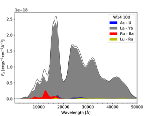
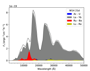
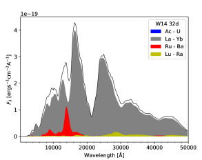
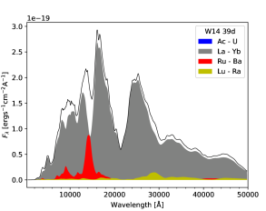
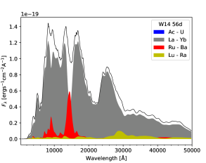
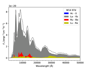
Figure 11: The W14 model spectra with element groups marked out. The contribution of actinides is found to be negligible at all epochs.

References

- Abbott et al. (2017) Abbott B. P., Abbott R., Abbott T. D., Acernese F., Ackley K., Adams C., Adams T., et al. 2017, ApJ, 848, L12
- Andres et al. (1996) Andres H. P., Krämer K., Güdel H. U., 1996, Phys. Rev. B, 54, 3830
- Axelrod (1980) Axelrod T. S., 1980, PhD thesis, California Univ., Santa Cruz.
- Barnes et al. (2016) Barnes J., Kasen D., Wu M.-R., Martínez-Pinedo G., 2016, ApJ, 829, 110
- Barnes et al. (2021) Barnes J., Zhu Y. L., Lund K. A., Sprouse T. M., Vassh N., McLaughlin G. C., Mumpower M. R., Surman R., 2021, ApJ, 918, 44
- Bromley et al. (2023) Bromley S. J., McCann M., Loch S. D., Ballance C. P., 2023, ApJS, 268, 22
- Bulla (2023) Bulla M., 2023, MNRAS, 520, 2558
- Bulla et al. (2019) Bulla M., et al., 2019, Nature Astronomy, 3, 99
- Carnall & Crosswhite (1985) Carnall W. T., Crosswhite H. M., 1985, Optical spectra and electronic structure of actinide ions in compounds and in solution
- Cowan et al. (2021) Cowan J. J., Sneden C., Lawler J. E., Aprahamian A., Wiescher M., Langanke K., Martínez-Pinedo G., Thielemann F.-K., 2021, Reviews of Modern Physics, 93, 015002
- Cowperthwaite et al. (2017) Cowperthwaite P. S., et al., 2017, ApJ, 848, L17
- Domoto et al. (2021) Domoto N., Tanaka M., Wanajo S., Kawaguchi K., 2021, ApJ, 913, 26
- Domoto et al. (2022) Domoto N., Tanaka M., Kato D., Kawaguchi K., Hotokezaka K., Wanajo S., 2022, ApJ, 939, 8
- Duflo & Zuker (1995) Duflo J., Zuker A. P., 1995, Phys. Rev. C, 52, R23
- Eichler et al. (1989) Eichler D., Livio M., Piran T., Schramm D. N., 1989, Nature, 340, 126
- Even et al. (2020) Even W., et al., 2020, ApJ, 899, 24
- Flörs et al. (2023) Flörs A., et al., 2023, MNRAS, 524, 3083
- Fontes et al. (2023) Fontes C. J., Fryer C. L., Wollaeger R. T., Mumpower M. R., Sprouse T. M., 2023, MNRAS, 519, 2862
- Freiburghaus et al. (1999) Freiburghaus C., Rosswog S., Thielemann F. K., 1999, ApJ, 525, L121
- Froese Fischer et al. (2019) Froese Fischer C., Gaigalas G., Jönsson P., Bieroń J., 2019, Computer Physics Communications, 237, 184
- Fujibayashi et al. (2020) Fujibayashi S., Wanajo S., Kiuchi K., Kyutoku K., Sekiguchi Y., Shibata M., 2020, ApJ, 901, 122
- Fujibayashi et al. (2023) Fujibayashi S., Kiuchi K., Wanajo S., Kyutoku K., Sekiguchi Y., Shibata M., 2023, ApJ, 942, 39
- Gaigalas et al. (2017) Gaigalas G., Froese Fischer C., Rynkun P., Jönsson P., 2017, Atoms, 5, 6
- Gillanders et al. (2021) Gillanders J. H., McCann M., Sim S. A., Smartt S. J., Ballance C. P., 2021, MNRAS, 506, 3560
- Gillanders et al. (2022) Gillanders J. H., Smartt S. J., Sim S. A., Bauswein A., Goriely S., 2022, MNRAS, 515, 631
- Giuliani et al. (2020) Giuliani S. A., Martínez-Pinedo G., Wu M.-R., Robledo L. M., 2020, Phys. Rev. C, 102, 045804
- Goriely et al. (2011) Goriely S., Bauswein A., Janka H.-T., 2011, ApJ, 738, L32
- Goriely et al. (2015) Goriely S., Bauswein A., Just O., Pllumbi E., Janka H. T., 2015, MNRAS, 452, 3894
- Gu (2008) Gu M. F., 2008, Canadian Journal of Physics, 86, 675
- Holmbeck et al. (2023) Holmbeck E. M., Barnes J., Lund K. A., Sprouse T. M., McLaughlin G. C., Mumpower M. R., 2023, ApJ, 951, L13
- Hotokezaka & Nakar (2020) Hotokezaka K., Nakar E., 2020, ApJ, 891, 152
- Hotokezaka et al. (2021) Hotokezaka K., Tanaka M., Kato D., Gaigalas G., 2021, MNRAS, 506, 5863
- Hotokezaka et al. (2022) Hotokezaka K., Tanaka M., Kato D., Gaigalas G., 2022, MNRAS, 515, L89
- Hotokezaka et al. (2023) Hotokezaka K., Tanaka M., Kato D., Gaigalas G., 2023, MNRAS, 526, L155
- Jerkstrand et al. (2011) Jerkstrand A., Fransson C., Kozma C., 2011, A&A, 530, A45
- Jerkstrand et al. (2012) Jerkstrand A., Fransson C., Maguire K., Smartt S., Ergon M., Spyromilio J., 2012, A&A, 546, A28
- Karbowiak (2005) Karbowiak M., 2005, Journal of Physical Chemistry A, 109, 3569
- Kasen & Barnes (2019) Kasen D., Barnes J., 2019, ApJ, 876, 128
- Kasen et al. (2017) Kasen D., Metzger B., Barnes J., Quataert E., Ramirez-Ruiz E., 2017, Nature, 551, 80
- Kasliwal et al. (2022) Kasliwal M. M., et al., 2022, MNRAS, 510, L7
- Kawaguchi et al. (2021) Kawaguchi K., Fujibayashi S., Shibata M., Tanaka M., Wanajo S., 2021, ApJ, 913, 100
- Kawaguchi et al. (2024) Kawaguchi K., Domoto N., Fujibayashi S., Hayashi K., Hamidani H., Shibata M., Tanaka M., Wanajo S., 2024, arXiv e-prints, p. arXiv:2404.15027
- Korobkin et al. (2012) Korobkin O., Rosswog S., Arcones A., Winteler C., 2012, MNRAS, 426, 1940
- Kramida et al. (2020) Kramida A., Yu. Ralchenko Reader J., and NIST ASD Team 2020, NIST Atomic Spectra Database (ver. 5.8), [Online]. Available: https://physics.nist.gov/asd [2021, September 22]. National Institute of Standards and Technology, Gaithersburg, MD.
- Kullmann et al. (2022) Kullmann I., Goriely S., Just O., Ardevol-Pulpillo R., Bauswein A., Janka H. T., 2022, MNRAS, 510, 2804
- Kullmann et al. (2023) Kullmann I., Goriely S., Just O., Bauswein A., Janka H. T., 2023, MNRAS, 523, 2551
- Lattimer & Schramm (1974) Lattimer J. M., Schramm D. N., 1974, ApJ, 192, L145
- Lattimer & Schramm (1976) Lattimer J. M., Schramm D. N., 1976, ApJ, 210, 549
- Lemaître et al. (2021) Lemaître J. F., Goriely S., Bauswein A., Janka H. T., 2021, Phys. Rev. C, 103, 025806
- Levan et al. (2024) Levan A. J., et al., 2024, Nature, 626, 737
- Madonna et al. (2018) Madonna S., et al., 2018, ApJ, 861, L8
- Mendoza-Temis et al. (2015) Mendoza-Temis J. d. J., Wu M.-R., Langanke K., Martínez-Pinedo G., Bauswein A., Janka H.-T., 2015, Phys. Rev. C, 92, 055805
- Möller et al. (1995) Möller P., Nix J. R., Myers W. D., Swiatecki W. J., 1995, Atomic Data and Nuclear Data Tables, 59, 185
- Mulholland et al. (2024) Mulholland L. P., McElroy N. E., McNeill F. L., Sim S. A., Ballance C. P., Ramsbottom C. A., 2024, MNRAS, 532, 2289
- Nedora et al. (2021) Nedora V., et al., 2021, ApJ, 906, 98
- Pognan et al. (2022a) Pognan Q., Jerkstrand A., Grumer J., 2022a, MNRAS, 510, 3806
- Pognan et al. (2022b) Pognan Q., Jerkstrand A., Grumer J., 2022b, MNRAS, 513, 5174
- Pognan et al. (2023) Pognan Q., Grumer J., Jerkstrand A., Wanajo S., 2023, MNRAS, 526, 5220
- Rastinejad et al. (2022) Rastinejad J. C., et al., 2022, Nature, 612, 223
- Rosswog & Korobkin (2022) Rosswog S., Korobkin O., 2022, arXiv e-prints, p. arXiv:2208.14026
- Rosswog et al. (1999) Rosswog S., Liebendörfer M., Thielemann F. K., Davies M. B., Benz W., Piran T., 1999, A&A, 341, 499
- Rosswog et al. (2017) Rosswog S., Feindt U., Korobkin O., Wu M. R., Sollerman J., Goobar A., Martinez-Pinedo G., 2017, Classical and Quantum Gravity, 34, 104001
- Roy & Prasad (2020) Roy S. K., Prasad R., 2020, Chemical Physics, 535, 110781
- Ruipérez et al. (2007) Ruipérez F., Roos B. O., Barandiarán Z., Seijo L., 2007, Chemical Physics Letters, 434, 1
- Sarin & Rosswog (2024) Sarin N., Rosswog S., 2024, arXiv e-prints, p. arXiv:2404.07271
- Seijo & Barandiarán (2003) Seijo L., Barandiarán Z., 2003, J. Chem. Phys., 118, 5335
- Shibata & Hotokezaka (2019) Shibata M., Hotokezaka K., 2019, Annual Review of Nuclear and Particle Science, 69, 41
- Smartt et al. (2017) Smartt S. J., et al., 2017, Nature, 551, 75
- Sneppen & Watson (2023) Sneppen A., Watson D., 2023, A&A, 675, A194
- Symbalisty & Schramm (1982) Symbalisty E., Schramm D. N., 1982, Astrophys. Lett., 22, 143
- Tanaka et al. (2018) Tanaka M., et al., 2018, ApJ, 852, 109
- Tanaka et al. (2020) Tanaka M., Kato D., Gaigalas G., Kawaguchi K., 2020, MNRAS, 496, 1369
- Tanvir et al. (2017) Tanvir N. R., et al., 2017, ApJ, 848, L27
- Tarumi et al. (2023) Tarumi Y., Hotokezaka K., Domoto N., Tanaka M., 2023, arXiv e-prints, p. arXiv:2302.13061
- Villar et al. (2017) Villar V. A., et al., 2017, ApJ, 851, L21
- Wanajo (2018) Wanajo S., 2018, ApJ, 868, 65
- Wanajo et al. (2014) Wanajo S., Sekiguchi Y., Nishimura N., Kiuchi K., Kyutoku K., Shibata M., 2014, ApJ, 789, L39
- Wanajo et al. (2022) Wanajo S., Fujibayashi S., Hayashi K., Kiuchi K., Sekiguchi Y., Shibata M., 2022, arXiv e-prints, p. arXiv:2212.04507
- Watson et al. (2019) Watson D., et al., 2019, Nature, 574, 497
- Waxman et al. (2019) Waxman E., Ofek E. O., Kushnir D., 2019, ApJ, 878, 93
- Wollaeger et al. (2018) Wollaeger R. T., et al., 2018, MNRAS, 478, 3298
- Wu & Banerjee (2022) Wu M.-R., Banerjee P., 2022, Association of Asia Pacific Physical Societies Bulletin, 32, 19
- Wu et al. (2016) Wu M.-R., Fernández R., Martínez-Pinedo G., Metzger B. D., 2016, MNRAS, 463, 2323
- Wu et al. (2019) Wu M.-R., Barnes J., Martínez-Pinedo G., Metzger B. D., 2019, Phys. Rev. Lett., 122, 062701
- Zhu et al. (2018) Zhu Y., et al., 2018, ApJ, 863, L23
- Zhu et al. (2021) Zhu Y. L., Lund K. A., Barnes J., Sprouse T. M., Vassh N., McLaughlin G. C., Mumpower M. R., Surman R., 2021, ApJ, 906, 94
- van Regemorter (1962) van Regemorter H., 1962, ApJ, 136, 906