A theory of generalised coordinates for stochastic differential equations

Abstract

Stochastic differential equations are ubiquitous modelling tools in physics and the sciences. In most modelling scenarios, random fluctuations driving dynamics or motion have some non-trivial temporal correlation structure, which renders the SDE non-Markovian; a phenomenon commonly known as “colored” noise. Thus, an important objective is to develop effective tools for mathematically and numerically studying (possibly non-Markovian) SDEs.

In this report, we formalise a mathematical theory for analysing and numerically studying SDEs based on so-called ‘generalised coordinates of motion’. Like the theory of rough paths, we analyse SDEs pathwise for any given realisation of the noise, not solely probabilistically. Like the established theory of Markovian realisation, we realise non-Markovian SDEs as a Markov process in an extended space. Unlike the established theory of Markovian realisation however, the Markovian realisations here are accurate on short timescales and may be exact globally in time, when flows and fluctuations are analytic.

This theory is exact for SDEs with analytic flows and fluctuations, and is approximate when flows and fluctuations are differentiable. It provides useful analysis tools, which we employ to solve linear SDEs with analytic fluctuations. It may also be useful for studying rougher SDEs, as these may be identified as the limit of smoother ones.

This theory supplies effective, computationally straightforward methods for simulation, filtering and control of SDEs; amongst others, we re-derive generalised Bayesian filtering, a state-of-the-art method for time-series analysis.

Looking forward, this report suggests that generalised coordinates have far-reaching applications throughout stochastic differential equations.

Introduction

Stochastic differential equations

Stochastic differential equations are ubiquitous tools in applied mathematics, physics and the sciences. Physically speaking, a stochastic differential equation

$$\frac{d}{dt}x_{t}=f(x_{t})+w_{t},$$ (1)

expresses the fact that a system $x_{t}$ exhibits slowly varying coarse behaviour described by a vector field $f$ superimposed with rapid random fluctuating motions $w_{t}$ and inherits from an adiabatic approximation (i.e. a time-scale separation) between fast and slow degrees of freedom [1]. In modelling, one can motivate a stochastic differential equation as describing how a system evolves when subjected to a combination of deterministic (known) and random (unknown) fluctuations. Stochastic differential equations are ubiquitous in physics—specifically in statistical, quantum or classical mechanics—as well as in many branches of applied mathematics, as a model of random dynamical systems.

White noise SDEs

Despite this intuitive view, the mathematical development of stochastic differential equations has been very challenging and a major endeavour of mathematics and physics since the early 20th century. The first mathematical theories of stochastic differential equations, due to Ito in the 1940s and later Stratonovich, were developed for the rigorous study of Brownian motion and related (Markovian) diffusion equations, which stand for ’white’ noise fluctuations $w_{t}$ in (1), and which can be motivated as a model of the motion of particles subject to thermal random fluctuations and other forces [2, 3, 4].

Colored noise SDEs

Beyond thermal fluctuations, random fluctuations in physics and in complex systems modelling are usually “coloured”: this is to say that fluctuations $w_{t}$ have some temporal correlation structure—think for instance of waves in the ocean and fluctuations in the wind. These coloured fluctuations make the solution to the SDE a non-Markovian process. With the limitations of white noise in mind, three main theories have been developed for analysing SDEs driven by coloured noise:

• The theory of stochastic differential equations driven by semi-martingales [5]: a theory of stochastic integration with respect to general (semi-martingale) noise processes, that extends Ito and Stratonovich calculus.

• The modern theory of stochastic differential equations driven by rough paths [6, 7], which analyses SDEs driven by general noise signals of possibly very low regularity. Contrasting with the other theories, this is an analytic theory in the sense that SDEs are analysed pathwise—that is for any given realisation of the noise—rather than simply probabilistically.

• The theory of Markovian realisation, which approximates non-Markovian processes by Markovian ones [8, 9, 10]. As a primary use case, this theory allows one to approximate coloured noise driven SDEs by white noise driven SDEs evolving in an extended state-space [4, Ch. 8], [2]. In particular, this approximation can be carried out for systems of non-Markovian interacting particles and their mean-field limit [11, 12], as well as for coloured multiplicative noise [13]. The resulting Markovian approximation is nevertheless quite challenging to analyse [14] as its generator and Fokker-Planck operator are necessarily degenerate (usually hypoelliptic and hypocoercive) [15].

To set the stage for this work, we draw attention to the scope of the current mathematical theory of Markovian realisation. As was noted by Stratonovich: “The study of Markov processes is particularly appropriate, since effective mathematical methods are available for analysing them. However, a certain care must be taken in replacing an actual process by Markov process, since Markov processes have many special features, and, in particular, differ from the processes encountered in radio engineering by their lack of smoothness” [16, p122]. It turns out that Markovian realisations furnish reasonable approximations to fluctuations over time-scales considerably larger than the correlation time; however, they fail at shorter timescales [16, p122]. “Thus the results obtained by applying the techniques of Markov process theory are valuable only to the extent to which they characterise just these ‘large-scale’ fluctuations. […] However, any random process actually encountered in radio engineering is analytic, and all its derivatives are finite with probability 1. Therefore, we cannot describe an actual process within the framework of Markov process theory, and the more accurately we wish to approximate such a process by a Markov process, the more components the latter must have and the higher the order of the corresponding fluctuation equation must be.” [16, p123-125].

A theory of generalised coordinates

In this paper, we present an alternative theory of Markovian realisation for stochastic differential equations based on generalised coordinates of motion; hereafter, “generalised coordinates”.

Scope: This is a theory for the analysis and numerical study of SDEs, which is exact for SDEs with analytic flows and fluctuations, and which is approximate when flows and fluctuations are differentiable. This theory may be applicable to rougher SDEs, as the Wong-Zakai theorems tell us that many of these can be expressed as limits of smoother SDEs. Like the theory of rough paths, we analyse SDEs pathwise for any given realisation of the noise, not solely probabilistically. Like the current theory of Markovian realisation we realise non-Markovian SDEs as a Markov process in an extended (possibly infinite dimensional) space. Unlike the established theory of Markovian realisation however, the Markovian realisations here are accurate on short timescales and may be exact globally in time, when flows and fluctuations are analytic. Crucially, this theory affords computationally straightforward methodologies for simulation, filtering and control of stochastic differential equations.

The basic idea: We can express the solution of a many times differentiable SDE by its Taylor expansion at any time point. (If the SDE’s coefficients are analytic we can consider the Taylor series). We can then reformulate the SDE as a dynamically-evolving Taylor expansion. If we define the coefficients of these Taylor expansions to be our generalised coordinates, the SDE becomes a linear ordinary differential equation in the high-dimensional space of generalised coordinates. We can then analyse the behaviour of this simpler dynamical system which (depending on context) gives us useful approximations or exact analytical solutions to the original equation. The question throughout is: how far can you go with Taylor expansions?

History: The use of generalised coordinates to analyse physical systems is ubiquitous in physics. To the best of our knowledge, the specific approach presented here was originally applied to SDEs as the basis of computationally straightforward and robust filtering of smooth time-series, specifically in the context of neuroimaging time-series obtained through functional magnetic resonance imaging [17, 18]. This approach has since percolated into other fields including robotics and control, where it showed state-of-the-art performance for i) radar tracking [19], ii) filtering during a real quadrotor flight experiment [20], iii) noise covariance estimation under coloured noise [21], and iv) system identification under coloured noise [22]. More recently, this approach was applied for analysing of SDEs in statistical physics, specifically in derivations of the free-energy principle [23, 24]. In this paper we formalise and develop these ideas, and show that they have far-reaching applications throughout stochastic differential equations.

Structure of paper

Chapter 1 sets the stage by explaining generalised coordinates for stochastic differential equations. We see how to reformulate an SDE to a dynamical system in generalised coordinates, and how to go back; and how much information about the initial SDE is preserved when applying this transform. We briefly review the Wong-Zakai theorems to delineate the class of SDEs where generalised coordinates might usefully be applied.

In Chapter 2, we delve deeper by examining basic analysis tools and results for stochastic differential equations using generalised coordinates. We start by analysing the statistical structure of random fluctuations in generalised coordinates, and then focus on the case where fluctuations are stationary Gaussian processes with many times differentiable sample paths. Under these conditions, we derive a comprehensive analysis of the solution to linear SDEs. Finally, we formulate the Fokker-Planck equation and the path integral formulation in generalised coordinates.

Chapter 3 develops numerical methods that make use of generalised coordinates. We start by numerical integration (“zigzag”) methods of SDEs that are accurate on short timescales. We then turn to an intriguing identity for numerically recovering the path of least action from the path integral formulation. Finally, we derive some new and existing methods for Bayesian filtering of time-series, variously known as generalised filtering. All of these numerical methods are supplemented with illustrative simulations and freely available code.

In Chapter 4, we briefly discuss ways in which this theory and numerical methods could be further developed, and provide concluding remarks. We also discuss our main omission from Chapter 3 which are methods for stochastic control using generalised coordinates. For reference, the Section A.1 has a glossary of some frequently used notations.

Chapter 1:  Fundaments of generalised coordinates

1.1 Realisation in generalised coordinates

1.1.1 The setup

Consider a stochastic differential equation on $\mathbb{R}^{d}$ over some open time interval $\mathbb{T}$ (which, without loss of generality contains $t=0$)

$$\frac{d}{dt}x_{t}=f(x_{t})+w_{t},\quad x_{0}=z\in\mathbb{R}^{d}.$$ (1.1)

The deterministic part is given by the drift or flow, a vector field $f:\mathbb{R}^{d}\to\mathbb{R}^{d}$, and the stochastic part is given by the random fluctuations or noise, a stochastic process $w:\mathbb{T}\times\Omega\to\mathbb{R}^{d}$. Here $\Omega$ denotes the sample space of the underlying probability space, made implicit throughout, so that we write $w_{t}\triangleq w(t,\cdot)$ for the random fluctuations at time $t$ (an $\mathbb{R}^{d}$-valued random variable).

Assumption 1.1.1 (Differentiability).

We assume there exists $N\in\mathbb{N}\backslash\{0\}\cup\{\infty\}$ such that the flow $f$ and the noise sample paths $t\mapsto w_{t}$ are $(N-1)$-times continuously differentiable (i.e., $f\in C^{N-1}(\mathbb{R}^{d},\mathbb{R}^{d})$ and $w(\cdot,\omega)\in C^{N-1}(\mathbb{T},\mathbb{R}^{d})$ for $\omega\in\Omega$ a.s.).

1.1.2 Motivation

We can express the motion of derivatives of the SDE (1.1), simply by differentiating w.r.t. time

$$\begin{split}\frac{d}{dt}x_{t}&=f(x_{t})+w_{t}\\ \frac{d^{2}}{dt^{2}}x_{t}&=\frac{d}{dt}f(x_{t})+\frac{d}{dt}w_{t}\\ &\vdots\\ \frac{d^{N}}{dt^{N}}x_{t}&=\frac{d^{N-1}}{dt^{N-1}}f(x_{t})+\frac{d^{N-1}}{dt^{N-1}}w_{t}\\ \end{split}$$ (1.2)

Fixing an initial time $t$ in (1.2)—without loss of generality $t=0$—yields a system of algebraic equations for the serial derivatives of the solution up to order $N$ at this time.

$$\begin{split}\frac{d}{dt}x_{t}\big{|}_{t=0}&=f(x_{0})+w_{0}\\ \frac{d^{2}}{dt^{2}}x_{t}\big{|}_{t=0}&=\frac{d}{dt}f(x_{t})\big{|}_{t=0}+\frac{d}{dt}w_{t}\big{|}_{t=0}\\ &\vdots\\ \frac{d^{N}}{dt^{N}}x_{t}\big{|}_{t=0}&=\frac{d^{N-1}}{dt^{N-1}}f(x_{t})\big{|}_{t=0}+\frac{d^{N-1}}{dt^{N-1}}w_{t}\big{|}_{t=0}\\ \end{split}$$ (1.3)

Assuming one can solve (1.3) we can approximately recover the solution trajectories of the SDE (1.2) from the serial derivatives via a Taylor expansion:

$$\begin{split}x_{t}&\approx\sum_{n=0}^{N}\frac{d^{n}}{dt^{n}}x_{t}\big{|}_{t=0}\frac{t^{n}}{n!}\\ \frac{d}{dt}x_{t}&\approx\sum_{n=0}^{N-1}\frac{d^{n+1}}{dt^{n+1}}x_{t}\big{|}_{t=0}\frac{t^{n}}{n!}\\ &\vdots\\ \frac{d^{N}}{dt^{N}}x_{t}&\approx\frac{d^{N}}{dt^{N}}x_{t}\big{|}_{t=0}\end{split}$$ (1.4)

Provided that the approximation by the Taylor expansion is sufficiently accurate, the typically hard problem of computing (or inferring) solution trajectories of SDEs yields to the much easier problem of computing (or inferring) serial derivatives of solutions at the time origin. It turns an uncountable number of equations—one (1.2) for each $t$—into a finite, or countably infinite, system of equations for $\frac{d}{dt}x_{t}\big{|}_{t=0},\ldots,\frac{d^{N}}{dt^{N}}x_{t}\big{|}_{t=0}$.

1.1.3 Generalised coordinates

This paper introduces a toolset for the analytic and numerical study of SDEs in this fashion. This requires embedding the SDE in a space of larger dimension, with auxiliary variables, which can be interpreted—in a first instance—as the position, velocity, acceleration, and higher order motion of the process. The goal will be to reformulate the SDE as a simple dynamical system in this higher dimensional space.

The space of generalised coordinates

The space of generalised coordinates of base dimension $d$ and order $n\in\mathbb{N}\cup\{\infty\}$ is

$$\mathbb{G}^{d,n}\triangleq\left\{\mathrm{z}^{(:n)}\triangleq\mathrm{z}^{(0:n)}\triangleq\begin{pmatrix}\mathrm{z}^{(0)}\\ \mathrm{z}^{(1)}\\ \vdots\\ \mathrm{z}^{(n)}\end{pmatrix}\mid\mathrm{z}^{(i)}\in\mathbb{R}^{d},\forall i=0,...,n\right\}\cong\mathbb{R}^{d(n+1)}$$ (1.5)

We treat elements of $\mathbb{G}^{d,n}$ as column vectors in $\mathbb{R}^{d(n+1)}$, which are finite or countably infinite dimensional depending on whether $n$ is finite or infinite.

The generalised flow

Reformulating (1.3) as an algebraic equation in generalised coordinates requires the following:

Claim: There exists functions $\mathrm{f}^{(n)}:\mathbb{G}^{d,n}\to\mathbb{R}^{d},n=0,\ldots,N-1$ such that for all $t\in\mathbb{T}$

$$\mathrm{f}^{(n)}\left(x_{t},\frac{d}{dt}x_{t},\ldots,\frac{d^{n}}{dt^{n}}x_{t}\right)\triangleq\frac{d^{n}}{dt^{n}}f(x_{t}).$$ (1.6)

Indeed, by the chain rule

$$\begin{split}\mathrm{f}^{(0)}\left(x_{t}\right)&=f(x_{t}),\quad\mathrm{f}^{(1)}\left(x_{t},\frac{d}{dt}x_{t}\right)=\nabla f(x_{t})\frac{d}{dt}x_{t}\\ \mathrm{f}^{(2)}\left(x_{t},\frac{d}{dt}x_{t}\right)&=\nabla f(x_{t})\frac{d^{2}}{dt^{2}}x_{t}+\left(\frac{d}{dt}x_{t}\right)^{\top}\nabla^{2}f(x_{t})\frac{d}{dt}x_{t}\\ &\vdots\end{split}$$ (1.7)

where the remaining $\mathrm{f}^{(n)}$ can be obtained analytically through repeated applications of the chain rule on $f$. Altogether, for $n\geq 1$

$$\mathrm{f}^{(n)}\left(x_{t},\frac{d}{dt}x_{t},\ldots,\frac{d^{n}}{dt^{n}}x_{t}\right)=\nabla f(x_{t})\frac{d^{n}}{dt^{n}}x_{t}+\text{terms involving higher order derivatives of }f$$ (1.8)

where these higher order terms vanish when $f$ is linear or $n=1$.

Definition 1.1.2 (Generalised flow).

The generalised flow is the function $\mathbf{f}:\mathbb{G}^{d,N}\to\mathbb{G}^{d,N-1}$

$$\mathbf{f}(\mathrm{z}^{(:N)})\triangleq\begin{pmatrix}\mathrm{f}^{(0)}\left(\mathrm{z}^{(0)}\right)\\ \mathrm{f}^{(1)}\left(\mathrm{z}^{(:1)}\right)\\ \vdots\\ \mathrm{f}^{(N-1)}\left(\mathrm{z}^{(:N-1)}\right)\end{pmatrix}$$ (1.9)

Note that the generalised flow is invariant w.r.t $\mathrm{z}^{(N)}$.

This approximation will be convenient at various stages later on:

Approximation 1.1.3 (Local linear approximation).

We say that we operate under the local linear approximation when we discard all contributions of derivatives of $f$ of order strictly higher than $1$.

Under the local linear approximation 1.1.3 the generalised flow equals:

$$\mathbf{f}(\mathrm{z}^{(:N)})=\begin{pmatrix}f\left(\mathrm{z}^{(0)}\right)\\ \nabla f(\mathrm{z}^{(0)})\mathrm{z}^{(1)}\\ \vdots\\ \nabla f(\mathrm{z}^{(0)})\mathrm{z}^{(N-1)}\end{pmatrix}$$ (1.10)

1.1.4 Formulation in generalised coordinates

We formulate a random dynamical system

$$\mathbf{x}_{t}\triangleq\mathrm{x}^{(:N)}_{t}\triangleq\mathrm{x}^{(0:N)}_{t}\triangleq\begin{pmatrix}\mathrm{x}^{(0)}_{t}\\ \mathrm{x}^{(1)}_{t}\\ \vdots\\ \mathrm{x}^{(N)}_{t}\end{pmatrix},\quad t\in\mathbb{T}$$ (1.11)

on the space of generalised coordinates $\mathbb{G}^{d,N}$ that captures the essential dynamics of the original SDE in the sense that it is equivalent to the RHS of (1.4) with (1.3) as initial condition.

$\mathbf{x}_{t}$ is defined as the unique solution to the generalised Cauchy problem

$$\begin{cases}\frac{d}{dt}\mathbf{x}_{t}=\mathbf{D}\mathbf{x}_{t}\\ \mathbf{D}^{\prime}\mathbf{x}_{0}=\mathbf{f}(\mathbf{x}_{0})+\mathbf{w}_{0}\\ \mathrm{x}^{(0)}_{0}=z\end{cases}$$ (1.12)

where

$$\begin{split}\mathbf{D}&\triangleq\underbrace{\operatorname{I}_{d}\otimes\overbrace{\begin{pmatrix}0&1&&&\\ &0&1&&\\ &&0&\ddots&\\ &&&\ddots&1\\ &&&&0\end{pmatrix}}^{\operatorname{Mat}_{N+1,N+1}}}_{\operatorname{Mat}_{(N+1)d,(N+1)d}},\quad\mathbf{D}^{\prime}\triangleq\underbrace{\operatorname{I}_{d}\otimes\overbrace{\begin{pmatrix}0&1&&&\\ &0&1&&\\ &&\ddots&\ddots&\\ &&&0&1\end{pmatrix}}^{\operatorname{Mat}_{N,N+1}}}_{\operatorname{Mat}_{Nd,(N+1)d}}\\ \mathbf{w}_{t}&\triangleq\mathrm{w}^{(:N-1)}_{t}\triangleq\mathrm{w}^{(0:N-1)}_{t}\triangleq\begin{pmatrix}\mathrm{w}^{(0)}_{t}\\ \mathrm{w}^{(1)}_{t}\\ \vdots\\ \mathrm{w}^{(N-1)}_{t}\end{pmatrix}\triangleq\begin{pmatrix}w_{t}\\ \frac{d}{dt}w_{t}\\ \vdots\\ \frac{d^{N-1}}{dt^{N-1}}w_{t}\end{pmatrix}\end{split}$$ (1.13)

so that $\mathbf{D}\mathbf{x}_{t}=(\mathrm{x}^{(1:N)}_{t}\>\>0)^{\top}\in\mathbb{G}^{d,N},\mathbf{D}^{\prime}\mathbf{x}_{0}=\mathrm{x}^{(1:N)}_{0}\in\mathbb{G}^{d,N-1},\mathbf{w}_{t}\in\mathbb{G}^{d,N-1}$. Note that the initial condition in (1.12) is equivalent to (1.3) with $x_{0}=z$. Furthermore, the dynamics in (1.12) are equivalent to saying that each coordinate $\mathrm{x}^{(n)}_{t}$ equals a Taylor polynomial centred at $t=0$ with coefficients $\mathrm{x}^{(n)}_{0},\ldots,\mathrm{x}^{(N)}_{0}$. Indeed, they are equivalent to

$$\begin{split}\mathbf{x}_{t}&=\exp(t\mathbf{D})\mathbf{x}_{0}\\ \exp(t\mathbf{D})&=\operatorname{I}_{d}\otimes\begin{pmatrix}1&t&t^{2}/2&\ldots&\frac{t^{N}}{N!}\\ &1&t&\ldots&\frac{t^{N-1}}{(N-1)!}\\ &&1&\ddots&\vdots\\ &&&\ddots&t\\ &&&&1\end{pmatrix}\end{split}$$ (1.14)

so that $\mathrm{x}_{t}^{(n)}=\sum_{i=0}^{N-n}\mathrm{x}^{(i+n)}_{0}\frac{t^{i}}{i!}$ as in the RHS of (1.4). It is interesting to note that (1.14) can be read either as the solution to the ordinary differential equation in the first line of (1.12) or as a Taylor approximation to (1.1). That the two are equivalent here is the key insight that underwrites use of generalised coordinates of motion.

1.1.5 The full construct

Consider $N=\infty$. The following is an equivalent condition to that given by the generalised process solution to (1.12) to match the serial derivatives of the SDE (1.1) at some time $t$

$$\mathbf{x}_{t}\triangleq\begin{pmatrix}\mathrm{x}^{(0)}_{t}\\ \mathrm{x}^{(1)}_{t}\\ \vdots\end{pmatrix}=\begin{pmatrix}\frac{d}{dt}x_{t}\\ \frac{d^{2}}{dt^{2}}x_{t}\\ \vdots\\ \end{pmatrix}\iff\mathbf{D}^{\prime}\mathbf{x}_{t}=\mathbf{f}(\mathbf{x}_{t})+\mathbf{w}_{t}$$ (1.15)

where the right equation in (1.15) corresponds to (1.2). This characterisation will be convenient later on.

1.2 Faithfulness

We now look at the faithfulness of the formulation in generalised coordinates w.r.t. the original SDE. That is, to what extent and over which time interval the generalised Cauchy problem (1.12) accurately encodes the solutions of (1.1). Obviously this depends on the value of $N$ and how many times the solutions of (1.1) are differentiable, or whether they are analytic. So we mainly focus on the conditions for the regularity of the solutions to (1.1).

Throughout this section, we consider the solution of the SDE (1.1) pathwise, that is, we fix an element of the sample space $\omega\in\Omega$, so that the corresponding noise sample path is determined $t\mapsto w_{\omega,t}\triangleq w(t,\omega)$, and we consider the regularity of the corresponding solution $t\mapsto x_{\omega,t}\triangleq x(t,\omega)$. We can summarise our setup as an ordinary non-homogeneous differential equation:

$$\begin{split}\frac{d}{dt}x_{\omega,t}=F_{\omega}(t,x_{\omega,t}),\quad x_{\omega,0}=z\in\mathbb{R}^{d},\end{split}$$ (1.16)

where $F_{\omega}:\mathbb{T}\times\mathbb{R}^{d}\to\mathbb{R}^{d},F_{\omega}(t,x)\triangleq f(x)+w_{\omega,t}$. Furthermore, we will write $x_{\omega}\triangleq x(\cdot,\omega),w_{\omega}\triangleq w(\cdot,\omega)$ for solution and noise trajectories.

1.2.1 Many times differentiable solutions

Sufficient conditions

Theorem 1.2.1.

If $F_{\omega}$ is $C^{N-1}$ (i.e. $f$ and $w_{\omega}$ are $C^{N-1}$) for $N\in\mathbb{N},N\geq 2$ in a neighbourhood of $(0,z)$, the initial value problem (1.16) has a unique solution $x_{\omega}:(-R_{\omega},R_{\omega})\to\mathbb{R}^{d}$ for some radius $R_{\omega}>0$. Furthermore, $x_{\omega}\in C^{N}((-R_{\omega},R_{\omega}))$. The same holds with $N=1$ provided $f$ is also locally Lipschitz.

Proof.

Let $D\subset\mathbb{T}\times\mathbb{R}^{d}$ be a closed rectangle on which $F_{\omega}$ is $C^{1}$, containing $(0,z)$ in its interior. Then, $F_{\omega}(t,x)$ is Lipshitzian in $x$ for any fixed $t$ in this rectangle [25, Lemma 1, Chapter 1.10]. The Picard-Lindelof theorem guarantees a unique solution $x_{\omega}$ to the differential equation (1.16), defined on a time interval $t\in(-R_{\omega},R_{\omega})$ for some $R_{\omega}>0$ [26, Theorem I.3.1]. Furthermore, this solution is $C^{1}$. Proceeding iteratively as in (1.2), we obtain that the solution $x_{\omega}$ is $C^{N}$. We can repeat the proof in the case where $N=1$ and $f$ locally Lipschitz, as there exists a (possibly smaller) domain $D$ such that $F_{\omega}$ is $C^{0}$ and Lipschitzian in the space variable for any fixed $t$. ∎

Accuracy statement

The accuracy of the generalised coordinate reformulation of the SDE is a direct consequence of Taylor’s theorem. Under the conditions of Theorem 1.2.1, we have $\varepsilon_{\omega}>0$ such that for all $t\in(-\varepsilon_{\omega},\varepsilon_{\omega})$

$$\mathrm{x}^{(0)}_{\omega,t}=\sum_{n=0}^{N}\mathrm{x}^{(n)}_{\omega,0}\frac{t^{n}}{n!}=\sum_{n=0}^{N}\frac{d^{n}}{dt^{n}}x_{\omega,t}\big{|}_{t=0}\frac{t^{n}}{n!}=x_{\omega,t}+o_{\omega}(|t|^{N}).$$ (1.17)

where $\mathrm{x}^{(0)}_{\omega,t}$ is the solution to the generalised Cauchy problem (1.12) where we fixed the noise sample path $w_{\omega}$, and $o_{\omega}$ refers to the fact that the little-o remainder may also depend on $\omega$.

Thus, increasing the order $N$ yields improved approximations of $x_{\omega,t}$ on possibly smaller neighbourhoods of $t=0$. For any fixed neighbourhood however, it is possible that increasing $N$ decreases the quality of the approximation at non-zero points, e.g., as the Taylor polynomial blows up. This will be important to consider later in simulations (e.g. in numerical integration) as increasing $N$ does not necessarily yield more accurate results on a fixed time interval. It is only when the solutions of (1.1) are analytic that increasing the order surely yields a better approximation on any fixed (albeit sufficiently small) interval.

1.2.2 Analytic solutions

Sufficient conditions

Definition 1.2.2.

A function $f:\mathbb{R}^{d}\to\mathbb{R}^{d}$ is analytic on a domain $D\subseteq\mathbb{R}^{d}$ if, for any $y\in D$, there exist constants $b_{ij_{0}j_{1}\ldots j_{d}}$ $(i=1,\ldots,d;j_{1}\ldots j_{d}=0,1,2,\ldots)$ and $\delta>0$, such that for any $i\in\{1,\ldots,d\}$:

$$f(x)_{i}=\sum_{j_{1}\ldots j_{d}=0}^{\infty}b^{(i)}_{ij_{1}\ldots j_{d}}\left(x_{1}-y_{1}\right)^{j_{1}}\ldots\left(x_{d}-y_{d}\right)^{j_{d}}\quad$$ (1.18)

provided that $\left|x_{1}-y_{1}\right|<\delta,\ldots,\left|x_{d}-y_{d}\right|<\delta.$

The definition of analyticity for $F_{\omega}:\mathbb{T}\times\mathbb{R}^{d}\to\mathbb{R}^{d}$ can be stated analogously. Obviously, the noise $w_{\omega,t}$ and the flow $f$ are analytic on domains $U_{w}\subset\mathbb{T},U_{f}\subset\mathbb{R}^{d}$, if and only if $F_{\omega}$ is analytic on $U_{w}\times U_{f}\subset\mathbb{T}\times\mathbb{R}^{d}$.

We now state a special case of a classic theorem due to Cauchy [27] and Kovalevskaya [28].

Theorem 1.2.3 (Cauchy–Kovalevskaya).

If $F_{\omega}$ is analytic (i.e. $f$ and $w_{\omega}$ are analytic) in a neighbourhood of $(0\>\>z)$, then the initial value problem (1.16) has a unique solution $x_{\omega}:(-R_{\omega},R_{\omega})\to\mathbb{R}^{d}$ for some $R_{\omega}>0$. Furthermore, $x_{\omega}$ is analytic on $(-R_{\omega},R_{\omega})$.

As usual, a function $f:D\subset\mathbb{R}^{d}\to\mathbb{R}^{d}$ is analytic if and only if it can be extended to a complex holomorphic function $f:D^{\prime}\subset\mathbb{C}^{d}\to\mathbb{C}^{d}$ (where $D^{\prime}\supset D$). This means that when $F_{\omega}$ is analytic around $(0,z)$, the initial value problem (1.16) can be extended to the complex plane. Complex analysis then provides an additional toolset to analyse these equations, cf. [29, Chapter 4].

Proof.

Uniqueness of solutions is guaranteed by the Picard-Lindelof theorem [26, Theorem I.3.1]. Existence of an analytic solution can be shown in at least two ways and we provide references below:

• [25, Theorem 5, p127] proves the result through the classical method of analytic majorisation: 1) finding a formal power series solution, and then showing (through a majorisation argument) that it has a positive radius of convergence. The argument is made for $d=1$, but it generalises to arbitrary $d$.

• [29, Theorem 4.2] proves the result for the equivalent initial value problem on the complex domain, exploiting the fact that the Picard iterates—in the proof of Picard iteration—are analytic and converge to an analytic function.

∎

Accuracy statement

Under the conditions of Theorem 1.2.3, $N=\infty$ implies that the generalised coordinate solution coincides with the original SDE solution

$$\mathrm{x}^{(0)}_{\omega,t}=\sum_{n=0}^{\infty}\mathrm{x}^{(n)}_{\omega,0}\frac{t^{n}}{n!}=\sum_{n=0}^{\infty}\frac{d^{n}}{dt^{n}}x_{\omega,t}\big{|}_{t=0}\frac{t^{n}}{n!}=x_{\omega,t}$$ (1.19)

over some time interval $t\in(-R_{\omega},R_{\omega})$. The question now is, what is the radius $R_{\omega}>0$ and can that be expressed uniformly in $\omega$?

• We will give an uniform value for $R_{\omega}$ for the linear SDE driven by a stationary Gaussian process with analytic sample paths in Section 2.2.2.

• In the non-linear $f$ case, [29, Theorem 4.1] gives a tight (non-uniform in $\omega$) lower bound on $R_{\omega}$, however this requires first extending and analysing $F_{\omega}$ (and thus $w_{\omega}$) in the complex domain, which may be impractical. Relevant here is also the Cauchy–Kovalevskaya bound on the radius of the solutions of analytic PDEs [30, Theorem 9.4.5], also non-uniform in $\omega$.

• Lastly, the following simple example shows that even though the coefficients of an ODE such as (1.16) may be entire, the solution may have an arbitrarily small radius of analyticity $R_{\omega}$:

  Example 1.2.4.

  The one-dimensional differential equation $\dot{x}_{t}=1+x^{2}_{t}$ with initial condition $x_{0}=z\in\mathbb{R}$ has a unique solution $x_{t}=\tan(t+c)$, where $c=c(z)=\tan^{-1}z\in(-\pi/2,\pi/2)$. Its maximal domain of definition around the time origin is $(-\pi/2-c,\pi/2-c)$. Its radius of convergence around the time origin is therefore $R(z)=\min\{|-\pi/2-c|,\pi/2-c\}$. In particular, $z\nearrow+\infty$ implies $c(z)\nearrow\pi/2$ and $R(z)\searrow 0$. This holds despite the fact that the radius of convergence of the flow $F_{\omega}(t,x)=1+x^{2}$ is infinite.

  See also [29, p. 113] for an example where the ODE solution is defined for all $t\geq 0$ but its radius of convergence can be made arbitrarily small. These non-examples remove the hope that the generalised coordinate solution $\mathbf{x}$ always exists globally in time when the flow $f$ and random fluctuations $w$ are entire almost surely.

1.3 Usefulness

We now observe that the generalised coordinate formulation (1.12) can be used to approximate the solutions of a wide range of stochastic differential equations with possibly singular drift and rough noise. Indeed, given an SDE with a (possibly singular) flow $f$ driven by (possibly rough) noise fluctuations $w$, there usually is an approximating SDE of the form (1.1) with analytic flow and fluctuations—for which the reformulation in generalised coordinates (1.12) is exact by Section 1.2.2.

The intuition is that many types of noise can be approximated by noises with analytic sample paths through smoothing. The smoothing operation here is convolution with a Gaussian, whereby if a noise process is smoothed in this way, one can recover it—or approximate it arbitrarily well—by letting the Gaussian standard deviation tend to zero. Intuitively, two SDEs with noises that are arbitrarily close and that are identical otherwise should produce solutions that are arbitrarily close. The same ideas go for approximating the drift in SDEs through smoothing.

1.3.1 Analytic approximation of noise

We now formalise these intuitions by showing sufficient conditions under which Gaussian convolution yields analytic sample paths.

The case of white noise

White noise is the prototypical example of random fluctuations in stochastic differential equations, due to their long history as an idealised model of thermal molecular noise [3].

Definition 1.3.1 (White noise, informal).

White noise $\omega_{t}$ is a mean-zero (stationary) Gaussian process on $t\in\mathbb{R}$ with autocovariance $\mathbb{E}[\omega_{t}\omega_{s}]=\delta(t-s)$ where $\delta$ is the Dirac delta function.

In this section, we consider the example of white noise convolved with a Gaussian

$$w_{t}=\int_{\mathbb{R}}\omega_{s}\phi({t-s})ds,\quad t\in\mathbb{R},\quad\phi_{t}\triangleq\phi(t)\triangleq(\sqrt{2\pi}\sigma)^{-1}e^{-\frac{t^{2}}{2\sigma^{2}}}$$ (1.20)

where $\sigma>0$ is the standard deviation parameter. Formally, as $\sigma\searrow 0$, $\phi\to\delta$ and thus $w_{t}\to\omega_{t}$.

Gaussian convolved white noise (1.20) is a mean-zero stationary Gaussian process with autocovariance

$$\begin{split}\mathbb{E}[w_{t}w_{t+h}]&=\mathbb{E}\left[\int_{\mathbb{R}}\omega_{s}\phi_{t-s}ds\int_{\mathbb{R}}\omega_{\tau}\phi_{t+h-\tau}d\tau\right]\\ &=\int_{\mathbb{R}}\int_{\mathbb{R}}\phi_{t-s}\phi_{t+h-\tau}\mathbb{E}[w_{s}w_{\tau}]dsd\tau\\ &=\int_{\mathbb{R}}\phi_{t-s}\phi_{t+h-s}ds\\ &=\frac{1}{2\pi\sigma^{2}}\int_{\mathbb{R}}e^{-\frac{(t-s)^{2}}{2\sigma^{2}}-\frac{(t+h-s)^{2}}{2\sigma^{2}}}ds\\ &=\frac{1}{2\pi\sigma^{2}}e^{-\frac{h^{2}}{4\sigma^{2}}}\int_{\mathbb{R}}e^{-\frac{\left(s-(t+h/2)\right)^{2}}{\sigma^{2}}}ds\\ &=\frac{1}{2\sqrt{\pi}\sigma}e^{-\frac{h^{2}}{4\sigma^{2}}}\end{split}$$ (1.21)

where the last line follows from the well-known value of the Gaussian integral.

Lemma 1.3.2.

Gaussian convolved white noise (1.20) has the power series representation

$$w_{\sqrt{2}\sigma t}\stackrel{{\scriptstyle\ell}}{{=}}(4\pi\sigma^{2})^{-\frac{1}{4}}e^{-\frac{t^{2}}{2}}\sum_{n=0}^{\infty}\frac{t^{n}}{\sqrt{n!}}\xi_{n},\quad t\in\mathbb{R},$$ (1.22)

where $\xi_{n}\sim\mathcal{N}(0,1),n\in\mathbb{N}$, are i.i.d. standard normal random variables and $\stackrel{{\scriptstyle\ell}}{{=}}$ denotes equality in law.

Proof.

First, we define

$$y_{t}\triangleq(4\pi\sigma^{2})^{-\frac{1}{4}}e^{-\frac{t^{2}}{2}}\sum_{n=0}^{\infty}\frac{t^{n}}{\sqrt{n!}}\xi_{n},\quad t\in\mathbb{R}.$$

Since the law of a Gaussian process is determined by the mean and autocovariance, we just need to show that 1) $y$ is a Gaussian process, 2) $y$ has the same mean as $w$, 3) $y$ has the same autocovariance as $w$. To do this we need the following basic fact about Gaussian random variables (which can be shown using Levy’s continuity theorem; cf. partial proofs here[31, 32]:

Fact 1.3.3.

Given $v_{n}\in\mathbb{R}^{m}$ for $n\in\mathbb{N}$, and $\sum_{n\geq 0}\left\|v_{n}\right\|^{2}<+\infty$, then $v\triangleq\sum_{n\geq 0}v_{n}\xi_{n}$ is an $m$-dimensional Gaussian random variable, with mean $\mathbb{E}[v]=0$ and covariance $\mathbb{E}\left[vv^{\top}\right]_{ij}=\sum_{n\geq 0}\left(v_{n}\right)_{i}\left(v_{n}\right)_{j}$.

1. Consider a finite sequence of times $t_{1},\ldots,t_{m}\in\mathbb{R}$, and define $v\triangleq(y_{t_{1}},\ldots,y_{t_{m}})$. Showing that $y$ is a Gaussian process amounts to showing that $v$ is joint normal. By construction

   $$v=\sum_{n\geq 0}v_{n}\xi_{n}\quad\text{where }v_{n}\in\mathbb{R}^{m},\>(v_{n})_{j}\triangleq(4\pi\sigma^{2})^{-\frac{1}{4}}e^{-{t_{j}^{2}}/{2}}\frac{t_{j}^{n}}{\sqrt{n!}}.$$

   To use the basic fact we observe that

   $$\begin{split}&\sum_{n\geq 0}\left\|v_{n}\right\|^{2}=\sum_{n\geq 0}\sum_{1\leq j\leq m}\left(2\sqrt{\pi}\sigma\right)^{-1}e^{-t_{j}^{2}}\frac{\left(t_{j}^{2}\right)^{n}}{n!}\\ =&\sum_{1\leq j\leq m}\left(2\sqrt{\pi}\sigma\right)^{-1}e^{-t_{j}^{2}}\sum_{n\geq 0}\frac{\left(t_{j}^{2}\right)^{n}}{n!}=\sum_{1\leq j\leq m}\left(2\sqrt{\pi}\sigma\right)^{-1}<\infty.\end{split}$$ (1.23)

   By the basic fact 1.3.3, $v$ is joint normal.

2. By the basic fact 1.3.3, $\mathbb{E}[v]=0$, so $y$ has zero-mean.

3. The basic fact 1.3.3 yields the autocovariance of $y$

   $$\mathbb{E}[y_{t}y_{s}] =\sum_{n\geq 0}(4\pi\sigma^{2})^{-\frac{1}{4}}e^{-\frac{t^{2}}{2}}\frac{t^{n}}{\sqrt{n!}}(4\pi\sigma^{2})^{-\frac{1}{4}}e^{-\frac{s^{2}}{2}}\frac{s^{n}}{\sqrt{n!}}$$

   $$=\left(2\sqrt{\pi}\sigma\right)^{-1}e^{-\frac{(t^{2}+s^{2})}{2}}\sum_{n\geq 0}\frac{(ts)^{n}}{\sqrt{n!}}$$

   $$=\left(2\sqrt{\pi}\sigma\right)^{-1}e^{-\frac{(t^{2}+s^{2})}{2}}e^{ts}=\left(2\sqrt{\pi}\sigma\right)^{-1}e^{-\frac{(t-s)^{2}}{2}}$$

   By inspection of (1.21) this is the autocovariance of $t\mapsto w_{\sqrt{2}\sigma t}$.

∎

Theorem 1.3.4.

Gaussian convolved white noise (1.20) $w_{t}$ extends to a process for $t\in\mathbb{C}$, with entire sample paths (i.e. analytic on $\mathbb{C}$), almost surely.

Proof.

We just need to show that the series (1.22) converges for every $t\in\mathbb{C}$ almost surely. It will then define an (almost surely) entire random function $\mathbb{C}\to\mathbb{C}$.

By Cauchy-Hadamard’s theorem [33, Theorem 2.5] the radius of convergence $R$ of the power series (1.22) is:

$$1/R=\limsup_{n\to\infty}\left|\frac{\xi_{n}}{\sqrt{n!}}\right|^{1/n}$$ (1.24)

Claim: We claim that $\frac{|\xi_{n}|}{\sqrt{n!}}\xrightarrow{n\to\infty}0$ almost surely.

The claim implies that $1/R=0$ and $R=+\infty$ almost surely.

Proof of claim. Note that $\frac{\xi_{n}}{\sqrt{n!}}$ is a mean-zero normal random variable with standard deviation $\frac{1}{\sqrt{n!}}$. Defining the sequence of events $A_{n}\triangleq\left\{\frac{|\xi_{n}|}{\sqrt{n!}}\geq\frac{1}{n}\right\},$ we have, by Chebyschev’s inequality:

$$\mathbb{P}(A_{n}) =\mathbb{P}\left(\frac{|\xi_{n}|}{\sqrt{n!}}\geq\frac{\sqrt{n!}}{n}\frac{1}{\sqrt{n!}}\right)\leq\frac{n^{2}}{n!}.$$

This implies $\sum_{n\geq 0}\mathbb{P}(A_{n})\leq\sum_{n\geq 0}\frac{n^{2}}{n!}<+\infty.$ The first Borel-Cantelli lemma then yields $\mathbb{P}\left(\liminf_{n\rightarrow\infty}A_{n}^{c}\right)=1,$ where $\liminf_{n\rightarrow\infty}A_{n}^{c}\triangleq\bigcup_{n=0}^{\infty}\bigcap_{k=n}^{\infty}\left\{\frac{|\xi_{n}|}{\sqrt{n!}}<\frac{1}{n}\right\}.$ In other words, with probability $1$, $\frac{|\xi_{n}|}{\sqrt{n!}}<\frac{1}{n}$ occurs for all but finitely many $n$. In particular, $\frac{|\xi_{n}|}{\sqrt{n!}}\to 0$ with probability $1.$ $\blacksquare$

Remark 1.3.5.

Note that the convergence of $\frac{|\xi_{n}|}{\sqrt{n!}}\to 0$ holds almost surely but not surely as any sequence of real numbers can be realised by $\frac{\xi_{n}}{\sqrt{n!}},n\geq 0$. However the set of sequences not converging to $0$ has probability zero. This shows that $w_{t}$ extends to the complex plane only almost surely, and thus all our future statements leveraging the analytic sample paths of Gaussian convolved white noise are almost sure statements.

∎

The case of integrable noise

Now consider an arbitrary noise process $w:\mathbb{T}\times\Omega\rightarrow\mathbb{R}$: we unpack conditions under which its sample paths are analytic when convolved with a Gaussian. For this, we fix an element of the sample space $\omega\in\Omega$, so that the corresponding noise sample path $w_{\omega}$ is determined.

Consider the Gaussian convolution

$$w_{\omega}*\phi:\mathbb{C}\to\mathbb{C},\>z\mapsto\int_{\mathbb{T}}w_{\omega,t}\phi(z-t)\>\mathrm{d}t,$$ (1.25)

where the Gaussian is given, without loss of generality (up to re-scaling of space and the convolution) by $\phi:\mathbb{C}\to\mathbb{C},z\mapsto e^{-z^{2}}$.

Remark 1.3.6.

Note that the Gaussian $\phi$ is unbounded on the complex plane

$$\phi(x+iy)=e^{-(x+iy)^{2}}=e^{-x^{2}-2ixy+y^{2}}=e^{-x^{2}+y^{2}}e^{-2ixy}\Rightarrow|\phi(x+iy)|=e^{-x^{2}+y^{2}}$$ (1.26)

but bounded on its compact subsets.

Question: under what conditions on the sample path $w_{\omega}$ is the convolution (1.25) well-defined?

Lemma 1.3.7.

Suppose that $w_{\omega}\in L^{1}(\mathbb{T})$, then (1.25) is well-defined (i.e. the integral converges).

Lemma 1.3.7 is relatively sharp given no further assumptions on the noise as the integral (1.25) may not converge for $w_{\omega}\in L^{1}_{\text{loc}}(\mathbb{T})$ and unbounded $\mathbb{T}$.

Proof of Lemma 1.3.7.

Let $z=x+iy\in\mathbb{C}$. By (1.26),

$$\left|\int_{\mathbb{T}}w_{\omega,t}\phi(z-t)\>\mathrm{d}t\right|\leq\int_{\mathbb{T}}|w_{\omega,t}\phi(z-t)|\>\mathrm{d}t=\int_{\mathbb{T}}|w_{\omega,t}|e^{-(x-t)^{2}+y^{2}}\>\mathrm{d}t\leq e^{y^{2}}\int_{\mathbb{T}}|w_{\omega,t}|\>\mathrm{d}t<\infty.$$

∎

Question: under what conditions on $w_{\omega}$ is the convolution (1.25) analytic on $\mathbb{T}$?

Proposition 1.3.8.

If $w_{\omega}\in L^{1}(\mathbb{T})$, then the convolution (1.25) is entire. In particular it is analytic on $\mathbb{T}$.

Proof of Proposition 1.3.8.

Consider the open squares:

$$\square_{n}\triangleq\{x+iy\in\mathbb{C}:x,y\in(-n,n)\}$$ (1.27)

Define the bump functions $b_{n}:\mathbb{C}\to\mathbb{R}$, with:

$$b_{n}\in C^{\infty}(\mathbb{R}^{2})\quad\text{and}\quad b_{n}(z)=\begin{cases}1\quad\text{when }z\in\square_{n}\\ \in[0,1]\quad\text{when }z\in\square_{n}^{c}\cap\square_{n+1}\\ 0\quad\text{when }z\in\square_{n+1}^{c}\end{cases}$$ (1.28)

By $b_{n}\in C^{\infty}(\mathbb{R}^{2})$ we mean that $b_{n}$ is smooth as a function of two real variables (not that it is holomorphic as a function of one complex variable). The superscript $c$ refers to the complement.

We define the approximations to the Gaussian

$$\phi_{n}\triangleq b_{n}\phi$$ (1.29)

It follows that

$$\begin{cases}\phi_{n}\xrightarrow{n\to\infty}\phi\text{ pointwise}\\ 0\leq|\phi_{n}|\leq|\phi_{n+1}|\leq\ldots\leq|\phi|\\ \phi_{n}\text{ has compact support}\\ \phi_{n}\in C^{\infty}(\mathbb{R}^{2})\\ \phi_{n}\text{ is holomorphic on }\square_{n}\end{cases}$$ (1.30)

Claim: The convolution $w_{\omega}*\phi_{n}:\mathbb{C}\to\mathbb{C},w*\phi_{n}(z)=\int_{\mathbb{T}}w_{\omega,t}\phi_{n}(z-t)\>\mathrm{d}t$ exists and is holomorphic on $\square_{n}$.

Proof of claim. Existence:

$$\int_{\mathbb{T}}|w_{\omega,t}\phi_{n}(z-t)|\>\mathrm{d}t\leq|\phi_{n}|_{L^{\infty}(\mathbb{C})}\int_{\mathbb{T}}|w_{\omega,t}|\>\mathrm{d}t\leq|\phi_{n}|_{L^{\infty}(\mathbb{C})}|w_{\omega}|_{L^{1}(\mathbb{T})}<\infty.$$ (1.31)

where $\phi_{n}\in L^{\infty}(\mathbb{C})$ follows from $\phi_{n}\in C^{\infty}(\mathbb{R}^{2})$ and $\phi_{n}$ has compact support.

Holomorphic on $\square_{n}$: since $\phi_{n}\in C^{\infty}(\mathbb{R}^{2})$ with compact support it is in particular Lipschitz continuous: $\exists C>0,\forall z,z^{\prime}\in\mathbb{C}$:

$$|\phi_{n}(z^{\prime})-\phi_{n}(z)|\leq C|z^{\prime}-z|.$$ (1.32)

Consider $z\in\square_{n}$:

$$\frac{d}{dz}(w_{\omega}*\phi_{n})(z)=\lim_{h\rightarrow 0}\int_{\mathbb{T}}w_{\omega,t}\frac{\phi_{n}(z+h-t)-\phi_{n}(z-t)}{h}\>\mathrm{d}t=\int_{\mathbb{T}}w_{\omega,t}\frac{d}{dz}\phi_{n}(z-t)\>\mathrm{d}t$$ (1.33)

where we moved the limit inside the integral by the dominated convergence theorem, as we have the domination

$$\left|w_{\omega,t}\frac{\phi_{n}(z+h-t)-\phi_{n}(z-t)}{h}\right|\leq|w_{\omega,t}|C,$$ (1.34)

by (1.32), the latter which is integrable on $\mathbb{T}$. In conclusion, $w_{\omega}*\phi_{n}$ is holomorphic on $\square_{n}$ and its complex derivative is given by (1.33). $\blacksquare$

Claim: The convolution $w_{\omega}*\phi_{n}$ converges to $w_{\omega}*\phi$ locally uniformly $\mathbb{C}$.

Proof of claim. It suffices to show uniform convergence on the closures $\overline{\square}_{m}$ for all $m\in\mathbb{N}$. In other words, letting $F,F_{n}:\mathbb{C}\to\mathbb{C},F_{n}\triangleq w*\phi_{n},F\triangleq w*\phi$ we must show that $\forall m\in\mathbb{N},\forall\varepsilon>0,\exists M\in\mathbb{N},\forall n\geq M,$

$$\sup_{z\in\overline{\square}_{m}}|F-F_{n}|(z)<\varepsilon.$$ (1.35)

Let $m\in\mathbb{N}$ and $\varepsilon>0$. Then,

$$\sup_{z\in\overline{\square}_{m}}|F-F_{n}|(z) \leq\int_{\mathbb{T}}|w_{\omega,t}|\sup_{z\in\overline{\square}_{m}}|\phi-\phi_{n}|(z-t)\>\mathrm{d}t\leq\sup_{z\in\overline{\square}_{m},t\in\mathbb{T}}|\phi-\phi_{n}|(z-t)\int_{\mathbb{T}}|w_{\omega,t}|\>\mathrm{d}t$$

$$=|w_{\omega}|_{L^{1}(\mathbb{T})}\sup_{\Im(z)\in[-m,m]}|\phi-\phi_{n}|(z).$$

where $\Im$ denotes the imaginary part. For $z=x+iy$ with $\Im(z)=y\in[-m,m]$ we have [by (1.26), (1.29)],

$$|\phi-\phi_{n}|(x+iy) \leq\mathds{1}_{\square_{n}^{c}}(x+iy)e^{-x^{2}+y^{2}}\leq e^{-n^{2}+m^{2}}.$$

Choosing $M\in\mathbb{N}$ large enough that $e^{-M^{2}+m^{2}}<\varepsilon/|w_{\omega}|_{L^{1}(\mathbb{T})}$ yields the result. $\blacksquare$

Now we use a well-known fact [34]:

Fact 1.3.9.

Let a domain $D\subset\mathbb{C}$ and a sequence of holomorphic functions $F_{n}:D\to\mathbb{C}$ that converges uniformly on compact subsets to $F:D\to\mathbb{C}$. Then $F$ is holomorphic on $D$.

Using the above fact shows that $w_{\omega}*\phi$ is holomorphic on $\square_{n}$ for any $n\in\mathbb{N}$. Since $n$ is arbitrary, $w_{\omega}*\phi$ is holomorphic on $\bigcup_{n\in\mathbb{N}}\square_{n}=\mathbb{C}$. ∎

Remark 1.3.10.

• If $\mathbb{T}$ is bounded then $C(\bar{\mathbb{T}})\subset L^{1}(\bar{\mathbb{T}})$, so any noise process $w$ with almost surely continuous sample paths becomes almost surely analytic on its domain when convolved with a Gaussian. For separable, stationary Gaussian processes on a compact interval, almost sure integrability and continuity of sample paths are equivalent [35, Theorem 1]).

• If $\mathbb{T}$ is unbounded and the process $w$ is non-zero and stationary, then one should not expect it to have samples in $L^{1}(\bar{\mathbb{T}})$; intuitively, stationarity implies that the sample paths behave the same everywhere, and thus the accumulated non-zero $L^{1}$ norms on any bounded interval add up to infinity on an unbounded time interval $\mathbb{T}$.

1.3.2 Analytic approximation of SDEs

After approximating many types of noises by analytic ones through Gaussian convolution, it begs the question: how do an initial and resulting approximating SDE relate? This is in essence the content of the Wong-Zakai theorems [36] and extensions thereof.

The Wong-Zakai theorem for white noise

The Wong-Zakai theorem [37, Theorem 2.8] says that for a sequence of piece-wise differentiable approximations $W_{\sigma,t}$ to an ($m$-dimensional) standard Wiener process $W_{t}$, in the sense that for every $T>0$,

$$\lim_{\sigma\searrow 0}\mathbb{E}\left[\sup_{0\leq t\leq T}\left|W_{t}-W_{\sigma,t}\right|^{2}\right]=0,$$ (1.36)

the solutions to the corresponding SDE

$$dx_{\sigma,t} =f\left(x_{\sigma,t}\right)dt+\varsigma dW_{\sigma,t},\quad x_{\sigma,0}=z$$ (1.37)

converge in the following sense

$$\lim_{\sigma\searrow 0}\mathbb{E}\left[\sup_{0\leq t\leq T}\left|x_{t}-x_{\sigma,t}\right|^{2}\right]=0,\quad\forall T>0,$$ (1.38)

to the solution of the limiting Stratonovich SDE

$$dx_{t} =f(x_{t})dt+\varsigma dW_{t},\quad x_{0}=z,$$ (1.39)

assuming that the noise is additive, i.e. $\varsigma\in\operatorname{Mat}_{d,m}$ is constant. In other words, the limit of the SDE (1.37) is the Stratonovich SDE (1.39) with the same drift and volatility. Crucially, [37, Theorem 2.8] gives a rate of convergence for (1.38). This applies to the preceding section on convolved white noise, whence

$$\begin{cases}\frac{d}{dt}x_{\sigma,t}=f\left(x_{\sigma,t}\right)+\varsigma\left(\omega*\phi_{\sigma}\right)_{t}\\ x_{\sigma,0}=z\end{cases}\xrightarrow{\sigma\searrow 0}\quad\begin{cases}\frac{d}{dt}x_{t}=f(x_{t})+\varsigma\omega_{t}\\ x_{0}=z\end{cases}$$

where convergence is pathwise in the sense of (1.38) and the Gaussian is $\phi_{\sigma}(t)=(\sqrt{2\pi}\sigma)^{-1}e^{-\frac{t^{2}}{2\sigma^{2}}}$.

All this means that we can use generalised coordinates to analyse stochastic differential equations driven by white noise, by smoothing the noise and analysing the resulting equation. When the flow is non-differentiable this needs to be smoothed as well for the approximating equation to have differentiable solutions. Luckily, there are also Wong-Zakai theorems for smooth approximations of the drift and the noise, e.g. [42].

The Wong-Zakai theorem for rough paths

But what about other types of rough noises that might be driving a stochastic differential equation? As there exists a fairly comprehensive theory for analysing SDEs driven by white noise, the appeal of generalised coordinates almost surely lies in offering analysis tools for SDEs driven by more complex and rough noises.

As it turns out, Wong-Zakai approximation theorems for SDEs driven by more complex rough paths have been studied extensively. Such rough processes include semi-martingales [43, 44], fractional Brownian motion [45, 46] and many other Gaussian processes [47], reversible Markov processes [48] as well as Markov processes with uniformly elliptic generator in divergence form [49, 50]. Nowadays, smooth approximations of SDEs driven by rough paths are best understood within the comprehensive theory of rough paths [51, 6, 7]. The idea is that there is a suitable topology on the space of paths (the rough path topology) such that the map sending a noise sample path to the corresponding solution of a stochastic differential equation (the Ito-Lyons map) is continuous [7, Theorem 8.5]. A general Wong-Zakai approximation theorem analoguous to (1.38) then follows trivially from this general result; see [51], [6, Section 17.4] and [7, Theorem 9.3].

Chapter 2:  Analysis in generalised coordinates

2.1 Generalised fluctuations

To be able to solve the generalised coordinate process $\mathbf{x}_{t}$ (1.12), we need knowledge about the random fluctuations in generalised coordinates $\mathbf{w}_{t}$ (1.13). In this section we ask: what are the statistics of generalised fluctuations?

2.1.1 Second order statistics

We consider wide-sense stationary noise processes $w$ that have $(N-1)$-times continuously differentiable sample paths, almost surely.

The noise assumption is generally taken to imply zero-mean $\mathbb{E}[w_{t}]=0,\forall t\in\mathbb{T}$ (as the mean can be added to the drift), so trivially $\mathbb{E}[\mathbf{w}_{t}]=0,\forall t\in\mathbb{T}$.

Consider the autocovariance function

$$\kappa(h)\triangleq\mathbb{E}[w_{t}w^{\top}_{t+h}]$$ (2.1)

which is independent of $t$ by the wide-sense stationarity assumption. Interestingly, the second order statistics of $\mathbf{w}$ can formally be expressed in terms of the serial derivatives of $\kappa$.

Lemma 2.1.1.

Formally, for $n,m=0,\ldots,N-1$

$$\mathbb{E}[\mathrm{w}^{(n)}_{t}\mathrm{w}^{(m)\top}_{t+h}]=(-1)^{n}\kappa^{(n+m)}(h)$$ (2.2)

where $\kappa^{(n+m)}(h)\triangleq\frac{d^{n+m}}{dh^{n+m}}\kappa(h)$.

Remark 2.1.2 (Formal calculation).

By ’formally’ we mean that the proof of Lemma 2.1.1 may need additional conditions on $w$ to hold in practice. Specifically, we do not justify the steps for getting the limit outside of the expectation in the first equality in (2.4) and (2.5). We will give sufficient conditions that make Lemma rigorous for Gaussian process $w$ in Section 2.1.2.

Proof of Lemma 2.1.1.

Claim:

$$\mathbb{E}[\mathrm{w}^{(0)}_{t}\mathrm{w}^{(m)\top}_{t+h}]=\kappa^{(m)}(h)$$ (2.3)

Proof of claim. We prove (2.3) by induction on $m$. The case $m=0$ is (2.1). We show the statement for $m\geq 1$ assuming it holds for $m-1$:

$$\begin{split}\mathbb{E}[\mathrm{w}^{(0)}_{t}\mathrm{w}^{(m)\top}_{t+h}]&=\lim_{s\to 0}\frac{1}{s}\mathbb{E}[\mathrm{w}_{t}(\mathrm{w}^{(m-1)\top}_{t+h+s}-\mathrm{w}^{(m-1)\top}_{t+h})]\\ &=\lim_{s\to 0}\frac{1}{s}\left(\kappa^{(m-1)}(h+s)-\kappa^{(m-1)}(h)\right)\\ &=\kappa^{(m)}(h).\end{split}$$ (2.4)

$\blacksquare$

Fix $m\geq 0$. We prove (2.2) by induction on $n$. The case $n=0$ is (2.3). We show the statement for $n\geq 1$ assuming it holds for $n-1$:

$$\begin{split}\mathbb{E}[\mathrm{w}^{(n)}_{t}\mathrm{w}^{(m)\top}_{t+h}]&=\lim_{s\to 0}\frac{1}{s}\mathbb{E}[(\mathrm{w}^{(n-1)}_{t+s}-\mathrm{w}^{(n-1)}_{t})\mathrm{w}^{(m)\top}_{t+h}]\\ &=\lim_{s\to 0}\frac{1}{s}\left(\mathbb{E}[\mathrm{w}^{(n-1)}_{t+s}\mathrm{w}^{(m)\top}_{t+h}]-\mathbb{E}[\mathrm{w}^{(n-1)}_{t}\mathrm{w}^{(m)\top}_{t+h}]\right)\\ &=(-1)^{n-1}\lim_{s\to 0}\frac{1}{s}\left(\kappa^{(n-1+m)}(h-s)-\kappa^{(n-1+m)}(h)\right)\\ &=(-1)^{n}\kappa^{(n+m)}(h).\end{split}$$ (2.5)

∎

(2.2) can be evaluated for any $2N-2$ times differentiable autocovariance function, and any $N-1$ times continuously differentiable noise $w$. Furthermore, Lemma 2.1.1 shows that $\mathbf{w}$ is wide-sense stationary if only if $w$ is wide-sense stationary. Therefore, the autocovariance of $\mathbf{w}$ is

$$\mathbb{E}[\mathbf{w}_{t}\mathbf{w}_{t+h}^{\top}]=\begin{bmatrix}\kappa(h)&\kappa^{(1)}(h)&\kappa^{(2)}(h)&\ldots\\ -\kappa^{(1)}(h)&-\kappa^{(2)}(h)&-\kappa^{(3)}(h)&\ldots\\ \kappa^{(2)}(h)&\kappa^{(3)}(h)&\kappa^{(4)}(h)&\ldots\\ \vdots&\vdots&\vdots&\ddots\end{bmatrix}\in\operatorname{Mat}_{Nd,Nd}.$$ (2.6)

The covariance of generalised fluctuations has a checkerboard structure, where odd temporal derivatives of $\kappa$ in (2.6) are replaced by zero submatrices. To see this, first note that the autocovariance of a wide-sense stationary process $h\mapsto\mathbb{E}[\mathrm{w}^{(n)}_{t}\mathrm{w}^{(n)\top}_{t+h}]$ attains a local maximum at $h=0$. By Lemma 2.1.1, this implies that $\kappa^{(2n)}(h)$ attains a local extremum at $h=0$. Thus, $\kappa^{(2n+1)}(0)=0$. We can find this result in another way: namely, by observing that the covariance of generalised fluctuations is symmetric. From (2.6),

$$\mathbb{E}[\mathbf{w}_{t}\mathbf{w}_{t}^{\top}]=\begin{bmatrix}\kappa(0)&0&\kappa^{(2)}(0)&\ldots\\ 0&-\kappa^{(2)}(0)&0&\ldots\\ \kappa^{(2)}(0)&0&\kappa^{(4)}(0)&\ldots\\ \vdots&\vdots&\vdots&\ddots\end{bmatrix}\in\operatorname{Mat}_{Nd,Nd}.$$ (2.7)

Example 2.1.3 (Gaussian autocovariance).

Consider the Gaussian autocovariance $\kappa(h)=(2\sqrt{\pi}\sigma)^{-1}e^{-\frac{h^{2}}{4\sigma^{2}}}$ (1.21) of Gaussian convolved white noise (1.20). By inspection,

$$\kappa^{(2n)}(0)=\frac{(-1)^{n}(2n-1)!!}{2^{n+1}\sqrt{\pi}\sigma^{2n+1}},\quad n\in\mathbb{N},$$

where $!!$ denotes the double factorial. In particular, the diagonal of the generalised covariance matrix (2.7) reads:

$$\frac{(2n-1)!!}{2^{n+1}\sqrt{\pi}\sigma^{2n+1}},\quad n=0,1,2,\ldots,N-1.$$

The white noise limit corresponds to the case $\sigma\searrow 0$, whence orders of motion higher than $n=0$ can be discarded with impunity.

Example 2.1.4 (Square rational autocovariance).

Suppose $\kappa(h)=\frac{1}{1+h^{2}}$. The Taylor series at the origin reads $\kappa(h)=\sum_{n=0}^{\infty}(-1)^{n}h^{2n}$ and converges for $|h|<1$. In particular, $\kappa^{(2n)}(0)=(-1)^{n}(2n)!$ and the diagonal of the matrix (2.7) reads $(2n)!$ for $n=0,1,2,\ldots,N-1$.

2.1.2 Gaussian process noise

We consider the preceding section in the context where the driving noise process $w$ is a Gaussian process (GP). In this case, the wide-sense stationarity assumption is equivalent to stationarity; we are thus in the setting of stationary GPs with $(N-1)$-times continuously differentiable sample paths a.s.. It turns out that we can make the calculations of the preceding Section 2.1.1 rigorous in this special setup.

Conditions for sample differentiability

First we must answer: what are the conditions on stationary GPs for the many times differentiability of their sample paths? In practice, Gaussian processes are often described and identified by their autocovariance (a.k.a. kernel) $\kappa$. Assuming zero mean, the regularity of the autocovariance determines the regularity of the GP sample paths almost surely [52]. Consider the following assumption:

Assumption 2.1.5 (Regular GP autocovariance).

$w$ is a mean-zero stationary Gaussian process with autocovariance $\kappa$ such that $\kappa^{(2(N-1))}$ exists and is locally Lipschitz continuous.

Note that, by the mean value theorem, the existence of one additional continuous derivative of $\kappa$ is sufficient for local Lipschitz continuity of the lower derivatives, and hence for Assumption 2.1.5. We have [52, Corollary 1]:

Proposition 2.1.6 (Sample differentiability of GPs).

Under Assumption 2.1.5, $w$ has $(N-1)$-times continuously differentiable sample paths almost surely. In other words, Assumption 2.1.5 implies Assumption 1.1.1.

Proposition 2.1.6 is sharper than alternative results in the existing literature, that, unlike this, derive the regularity conditions on the autocovariance via sample path regularity in Sobolev spaces and the Sobolev embedding theorems, which requires more derivatives [53].

In addition Assumption 2.1.5 implies a rigorous proof of Lemma 2.1.1 (see Remark 2.1.2) following the proof of the forward implication of [52, Theorem 7]. So:

Proposition 2.1.7.

Under Assumption 2.1.5,

$$\mathbb{E}[\mathrm{w}^{(n)}_{t}\mathrm{w}^{(m)\top}_{t+h}]=(-1)^{n}\kappa^{(n+m)}(h).$$ (2.8)

It follows that the calculations of the preceding section 2.1.1 are made rigorous under Assumption 2.1.5.

Gaussianity of generalised fluctuations

Now that we have established sufficient conditions on the autocovariance $\kappa$ for many times differentiability of the sample paths, we look at the structure of the generalised GP fluctuations $\mathbf{w}$.

Proposition 2.1.8.

Consider a mean-zero $\mathbb{R}^{d}$-valued Gaussian process $w$ with almost surely $(N-1)$-times continuously differentiable sample paths. Then, $\mathbf{w}$ is an $\mathbb{R}^{dN}$-valued Gaussian process.

Proof.

Consider the process $\mathrm{w}^{(0:n)}\triangleq(\mathrm{w}^{(0)},\ldots,\mathrm{w}^{(n)})$ for any $0\leq n\leq N-1$: we show that this is an $\mathbb{R}^{dn}$-valued Gaussian process by induction on $n$. The case $n=0$ holds by assumption. Suppose that the statement holds for $n=k$ for some arbitrary $k<N-1$. We show it for $n=k+1$. Consider some arbitrary finite set of times: $m\in\mathbb{N},t_{0},\ldots t_{m}\in\mathbb{T}$. For any $\varepsilon>0$

$$\left(\mathrm{w}_{t_{0}}^{(0)},\ldots,\mathrm{w}_{t_{m}}^{(0)},\ldots,\mathrm{w}_{t_{0}}^{(k)},\ldots,\mathrm{w}_{t_{m}}^{(k)},\frac{\mathrm{w}_{t_{0}+\varepsilon}^{(k)}-\mathrm{w}_{t_{0}}^{(k)}}{\varepsilon},\ldots,\frac{\mathrm{w}_{t_{m}+\varepsilon}^{(k)}-\mathrm{w}_{t_{m}}^{(k)}}{\varepsilon}\right)$$ (2.9)

is joint Gaussian. Indeed, (2.9) is a linear transformation of the random variable $\left(\mathrm{w}_{t_{0}}^{(0)},\ldots,\mathrm{w}_{t_{m}}^{(0)},\ldots,\mathrm{w}_{t_{0}}^{(k)},\ldots,\mathrm{w}_{t_{m}}^{(k)}\right)$, which is multivariate Gaussian by our induction hypothesis. (2.9) converges almost surely to

$$\left(\mathrm{w}_{t_{0}}^{(0)},\ldots,\mathrm{w}_{t_{m}}^{(0)},\ldots,\mathrm{w}_{t_{0}}^{(k)},\ldots,\mathrm{w}_{t_{m}}^{(k)},\mathrm{w}_{t_{0}}^{(k+1)},\ldots,\mathrm{w}_{t_{m}}^{(k+1)}\right)$$ (2.10)

as $\varepsilon\to 0$. Recall that almost sure convergence implies convergence in distribution (a.k.a. weak convergence). Therefore, we deduce that (2.10) is joint Gaussian [54, 55]. Since $t_{0},\ldots t_{m}$ are arbitrary, $\mathbf{w}$ is a Gaussian process. ∎

It follows that the generalised GP fluctuations $\mathbf{w}_{t}$ have a simple Gaussian form that is constant in time:

Theorem 2.1.9.

Under Assumption 2.1.5, the generalised GP fluctuations have the distribution

$$\mathbf{w}_{t}\sim\mathcal{N}(0,\mathbf{\Sigma}),\>\forall t\in\mathbb{T},$$ (2.11)

with covariance $\mathbf{\Sigma}$ given by (2.7).

Proof.

Under Assumption 2.1.5, Proposition 2.1.7 justifies all the calculations of Section 2.1.1, and in particular the covariance (2.7) and zero-mean. Furthermore, Assumption 2.1.5 implies Proposition 2.1.8, which implies that $\mathbf{w}_{t}$ is a multivariate Gaussian random variable. ∎

2.2 Analysis of the linear equation

In this section, we analyse the linear SDE driven by a stationary Gaussian process $w$ using generalised coordinates (i.e. (1.1) with linear flow $f$)

$$\frac{d}{dt}x_{t}=Ax+w_{t},\quad A\in\operatorname{Mat}_{d,d},\quad x_{0}=z\in\mathbb{R}^{d}.$$ (2.12)

2.2.1 Many times differentiable fluctuations

We operate under sufficient regularity on the noise autocovariance—i.e. Assumption 2.1.5—which implies a.s. many times differentiability of sample paths: i.e. Assumption 1.1.1, by Proposition 2.1.6.

The algebraic equation for relating the various derivatives of (2.12) at $t=0$ equals (1.12)

$$\begin{split}\mathrm{x}_{0}^{(1)}&=A\mathrm{x}_{0}^{(0)}+\mathrm{w}_{0}^{(0)}\\ \mathrm{x}_{0}^{(2)}&=A\mathrm{x}_{0}^{(1)}+\mathrm{w}_{0}^{(1)}\\ &\vdots\\ \mathrm{x}_{0}^{(N)}&=A\mathrm{x}_{0}^{(N-1)}+\mathrm{w}_{0}^{(N-1)}\\ \end{split}$$ (2.13)

By substitution the generalised coordinates at $t=0$ equal

$$\mathrm{x}_{0}^{(n)}=A^{n}\mathrm{x}_{0}^{(0)}+\sum_{k=0}^{n-1}A^{n-1-k}\mathrm{w}_{0}^{(k)},\quad\forall 1\leq n\leq N.$$ (2.14)

The deterministic initial condition $\mathrm{x}_{0}^{(0)}=z$ yields that the vector of generalised coordinates $\mathbf{x}_{0}$ is joint Gaussian (as an affine transform of the multivariate Gaussian random variable $\mathbf{w}_{0}$).

Thus the zero-th order generalised coordinate process

$$\mathrm{x}_{t}^{(0)}=\sum_{n=0}^{N}\mathrm{x}^{(n)}_{0}\frac{t^{n}}{n!},$$ (2.15)

which by construction approximates the solution to (2.12) is a Gaussian process.

Proposition 2.2.1.

Under Assumption 2.1.5, the Gaussian process (2.15) has mean and autocovariance

$$\begin{split}\mathbb{E}\left[\mathrm{x}_{t}^{(0)}\right]&=\sum_{n=0}^{N}A^{n}x_{0}\frac{t^{n}}{n!},\quad\operatorname{cov}(\mathrm{x}_{t}^{(0)},\mathrm{x}_{s}^{(0)})=\sum_{n,m=1}^{N}\frac{t^{n}s^{m}}{n!m!}\sum_{k=0}^{n-1}\sum_{l=0}^{m-1}A^{n-1-k}(-1)^{k}\kappa^{(k+l)}(0)(A^{m-1-l})^{\top}.\end{split}$$ (2.16)

Proof.

Using (2.14) at $t=0$ we have

$$\mathbb{E}[\mathrm{x}_{t}^{(0)}]=\mathbb{E}\left[\sum_{n=0}^{N}\mathrm{x}_{0}^{(n)}\frac{t^{n}}{n!}\right]=\mathbb{E}\left[\sum_{n=0}^{N}\left(A^{n}x_{0}+\sum_{k=0}^{n-1}A^{n-1-k}\mathrm{w}_{0}^{(k)}\right)\frac{t^{n}}{n!}\right]=\sum_{n=0}^{N}A^{n}x_{0}\frac{t^{n}}{n!}.$$ (2.17)

Furthermore,

$$\begin{split}\operatorname{cov}(\mathrm{x}_{t}^{(0)},\mathrm{x}_{s}^{(0)})&=\mathbb{E}\left[\left(\sum_{n=0}^{N}\mathrm{x}_{0}^{(n)}\frac{t^{n}}{n!}-\sum_{n=0}^{N}A^{n}x_{0}\frac{t^{n}}{n!}\right)\left(\sum_{n=0}^{N}\mathrm{x}_{0}^{(n)}\frac{s^{n}}{n!}-\sum_{n=0}^{N}A^{n}x_{0}\frac{t^{n}}{n!}\right)^{\top}\right]\\ &=\mathbb{E}\left[\sum_{n=1}^{N}\frac{t^{n}}{n!}\sum_{k=0}^{n-1}A^{n-1-k}\mathrm{w}_{0}^{(k)}\left(\sum_{n=1}^{N}\frac{s^{n}}{n!}\sum_{k=0}^{n-1}A^{n-1-k}\mathrm{w}_{0}^{(k)}\right)^{\top}\right]\\ &=\sum_{n,m=1}^{N}\frac{t^{n}s^{m}}{n!m!}\sum_{k=0}^{n-1}\sum_{l=0}^{m-1}A^{n-1-k}\mathbb{E}\left[\mathrm{w}_{0}^{(k)}\mathrm{w}_{0}^{(l)\top}\right](A^{m-1-l})^{\top}\\ &=\sum_{n,m=1}^{N}\frac{t^{n}s^{m}}{n!m!}\sum_{k=0}^{n-1}\sum_{l=0}^{m-1}A^{n-1-k}(-1)^{k}\kappa^{(k+l)}(0)(A^{m-1-l})^{\top}\end{split}$$ (2.18)

where we used Proposition 2.1.7 for the last line. ∎

2.2.2 Smooth and analytic fluctuations

Now we make an assumption that is strictly stronger than Assumption 2.1.5.

Assumption 2.2.2.

$w$ is a mean-zero stationary Gaussian process with smooth autocovariance $\kappa$.

By [52, Corollary 13], Assumption 2.2.2 is equivalent to $w$ having smooth sample paths, a stronger statement than Proposition 2.1.6 which solely yields the forward implication. We make this assumption so that we can consider the zero-th order coordinate process $\mathrm{x}^{(0)}$ (2.15) as $N\to\infty$.

Proposition 2.2.3.

Under Assumption 2.2.2, the mean of the zero-th coordinate process $\mathrm{x}^{(0)}$ (2.15) has the limit

$$\mathbb{E}\left[\mathrm{x}_{t}^{(0)}\right]\xrightarrow{N\to\infty}e^{At}x_{0}.$$ (2.19)

Proposition 2.2.3 is obvious from Proposition 2.2.1. Furthermore, this is exactly what we expect as this coincides with the mean of the linear diffusion process [56, eq. 2.7].

Now we consider the limiting behaviour of the autocovariance. For the limit to even exist we need a stronger assumption than 2.2.2:

Assumption 2.2.4.

The autocovariance $\kappa$ of the noise process $w$ in (2.12) is analytic around $0$ with radius of convergence $2R$.

From this assumption, we obtain the limit of the autocovariance of the zero-th order process:

Proposition 2.2.5.

Under Assumption 2.2.4,

$$\operatorname{cov}(\mathrm{x}_{t}^{(0)},\mathrm{x}_{s}^{(0)})\xrightarrow{N\to\infty}\sum_{n,m=1}^{\infty}\frac{t^{n}s^{m}}{n!m!}\sum_{k=0}^{n-1}\sum_{l=0}^{m-1}A^{n-1-k}(-1)^{k}\kappa^{(k+l)}(0)(A^{m-1-l})^{\top}$$ (2.20)

where the convergence is locally uniform in $t,s\in(-R/\lambda,R/\lambda)$, where $\lambda\triangleq\max(1,\|A\|_{\infty},\|A^{\top}\|_{\infty})$ and where $\|\cdot\|_{\infty}$ is the matrix operator norm induced by the vector $l^{\infty}$ norm, which equals the maximum absolute column sum $\|A\|_{\infty}\triangleq\max_{1\leq i\leq d}\sum_{j=1}^{d}|A_{ij}|.$

Remark 2.2.6.

We have $R/\lambda\geq R/(\alpha d)$ where $\alpha\triangleq\max(\{1\}\cup\{|A_{ij}|\}_{1\leq i,j\leq d})$.

Proof.

$\|\cdot\|_{\infty}$ is sub-multiplicative, so for $0\leq k\leq n-1$, $0\leq l\leq m-1$,

$$\left\|A^{n-1-k}(-1)^{k}\kappa^{(k+l)}(0)(A^{m-1-l})^{T}\right\|_{\infty} \leq\|A\|_{\infty}^{n-1-k}\|\kappa^{(k+l)}(0)\|_{\infty}\|A^{\top}\|_{\infty}^{m-1-l}$$

$$\leq\lambda^{n+m}\kappa_{n+m}.$$

where $\kappa_{n}\triangleq\max_{0\leq i\leq n}\|\kappa^{(i)}(0)\|_{\infty}$. From (2.16), we have the following upper bound on the autocovariance

$$|\operatorname{cov}(\mathrm{x}_{t}^{(0)},\mathrm{x}_{s}^{(0)})|\leq\sum_{n,m=1}^{N}\frac{|t|^{n}|s|^{m}}{n!m!}\left\|\sum_{k=0}^{n-1}\sum_{l=0}^{m-1}A^{n-1-k}(-1)^{k}\kappa^{(k+l)}(0)(A^{m-1-l})^{\top}\right\|_{\infty}\leq\sum_{n,m=1}^{N}|t|^{n}|s|^{m}\lambda^{n+m}\frac{nm\kappa_{n+m}}{n!m!}.$$ (2.21)

On the other hand, note that for $-R<t,s<R$, we have by Assumption 2.2.4

$$\mathbb{E}[\mathrm{w}^{(0)}_{t}\mathrm{w}^{(0)\top}_{s}]=\sum_{n,m=0}^{\infty}t^{n}s^{m}\frac{(-1)^{m}\kappa^{(n+m)}(0)}{n!m!}.$$ (2.22)

By the Cauchy-Hadamard theorem applied to (2.22),

$$\frac{1}{R}=\limsup_{\begin{subarray}{c}n+m\to\infty\\ n,m\geq 0\end{subarray}}\left(\frac{\|\kappa^{(n+m)}(0)\|_{\infty}}{n!m!}\right)^{\frac{1}{n+m}}\geq\limsup_{\begin{subarray}{c}n+m\to\infty\\ n,m\geq 1\end{subarray}}\left(\frac{\|\kappa^{(n+m)}(0)\|_{\infty}}{n!m!}\right)^{\frac{1}{n+m}}=\limsup_{\begin{subarray}{c}n+m\to\infty\\ n,m\geq 1\end{subarray}}\left(\frac{\kappa_{n+m}}{n!m!}\right)^{\frac{1}{n+m}},$$ (2.23)

where the last equality holds by a technical Lemma A.2.1 derived in Appendix A.2. Note that for $n,m\geq 1$ we have $n^{\frac{1}{n+m}},m^{\frac{1}{n+m}}\to 1$ as $n+m\to\infty$. We apply this to (2.23) to obtain

$$\limsup_{\begin{subarray}{c}n+m\to\infty\\ n,m\geq 1\end{subarray}}\left(\frac{nm\kappa_{n+m}}{n!m!}\right)^{\frac{1}{n+m}}\leq\frac{1}{R}.$$ (2.24)

Applying the Cauchy-Hadamard theorem and (2.24) to (2.21), yields that the majorising series for $|\operatorname{cov}(\mathrm{x}_{t}^{(0)},\mathrm{x}_{s}^{(0)})|$ converges absolutely for $-R/\lambda<t,s<R/\lambda$, and hence $\operatorname{cov}(\mathrm{x}_{t}^{(0)},\mathrm{x}_{s}^{(0)})$ converges as $N\to\infty$, locally uniformly within this radius, and the limit is analytic as it can be written as a power series. ∎

Now that we know the mean and autocovariance of the zero-th coordinate process (2.15) as $N\to\infty$, we just need to verify that the limiting process is a Gaussian process. It turns out that pointwise convergence of the autocovariance ensures weak convergence of the finite dimensional distributions of the zero-th coordinate process $\mathrm{x}^{(0)}_{t}$. Local uniform convergence of the autocovariance however, ensures the weak convergence in the sense of Gaussian processes, which is a stronger property.

Lemma 2.2.7.

Let $(g_{N})_{N\geq 1}$ be a sequence of Gaussian processes $g_{N}:I\times\Omega\to\mathbb{R}^{d}$, with $I\subset\mathbb{R}$ an interval, with almost surely continuous sample paths, with means $(\mu_{N})_{N\geq 1}$ and autocovariances $(k_{N})_{N\geq 1}$. If

1. $(\mu_{N})_{N\geq 1}$ converges pointwise,

2. $(k_{N})_{N\geq 1}$ converges locally uniformly to a continuous limit,

then $(g_{N})_{N\geq 1}$ converges weakly in $C(I,\mathbb{R}^{d})$ to a Gaussian process with mean $\lim_{N\to\infty}\mu_{N}$ and kernel $\lim_{N\to\infty}k_{N}$.

Proof.

1. and 2. imply that the finite dimensional distributions of the $g_{N}$ converge. So if $(g_{N})_{N\geq 1}$ converges weakly, it necessarily does so to the Gaussian process with mean $\lim_{N\to\infty}\mu_{N}$ and kernel $\lim_{N\to\infty}k_{N}$. First suppose $d=1$. Let $(t_{N})_{N\geq 1}\subset\mathbb{T}$ be a bounded sequence of times, and $(h_{N})_{N\geq 0}$ be a sequence of positive numbers tending to 0. Then

$$\mathbb{E}[|g_{N}(t_{N}+h_{N})-g_{N}(t_{N})|^{2}] =\mathbb{E}[g_{N}(t_{N}+h_{N})^{2}]+\mathbb{E}[g_{N}(t_{N})^{2}]-2\mathbb{E}(g_{N}(t_{N}+h_{N})g_{N}(t_{N})]$$

$$=k_{N}(t_{N}+h_{N},t_{N}+h_{N})+k_{N}(t_{N},t_{N})-2k_{N}(t_{N}+h_{N},t_{N})$$

$$=|k_{N}(t_{N}+h_{N},t_{N}+h_{N})-k_{\infty}(t_{N}+h_{N},t_{N}+h_{N})|$$

$$\;\;+|k_{N}(t_{N},t_{N})-k_{\infty}(t_{N},t_{N})|$$

$$\;\;+|2k_{N}(t_{N}+h_{N},t_{N})-2k_{\infty}(t_{N}+h_{N},t_{N})|$$

$$\;\;+|k_{\infty}(t_{N}+h_{N},t_{N}+h_{N})+k_{\infty}(t_{N},t_{N})-2k_{\infty}(t_{N}+h_{N},t_{N})|$$

$$\to 0\text{ as }N\to\infty$$

by uniform convergence of $(k_{N})_{N\geq 1}$ and uniform continuity of $k_{\infty}\triangleq\lim_{N\to\infty}k_{N}$ on $[\inf_{N\geq 1}(t_{N}),\sup_{N\geq 1}(t_{N}+h_{N})]\times[\inf_{N\geq 1}(t_{N}),\sup_{N\geq 1}(t_{N}+h_{N})]$. So $|g_{N}(t_{N}+h_{N})-g_{N}(t_{N})|$ tends to 0 in $L^{2}$, and in particular it converges in probability. Then [57, Theorem 14.5, 14.6 & 14.11] implies that $(g_{N})_{N\geq 1}$ converges weakly in $C(\mathbb{T},\mathbb{R})$, where we also used [57, Lemma 14.1] to view $g_{N}$ as random elements of $C(\mathbb{T},\mathbb{R})$.

For arbitrary $d\in\mathbb{N}$, note that $\mathbb{E}[\|g_{N}(t_{N}+h_{N})-g_{N}(t_{N})\|^{2}]=\sum_{i=1}^{d}\mathbb{E}[|g_{N}(t_{N}+h_{N})_{i}-g_{N}(t_{N})_{i}|^{2}]$, so the same proof strategy applies. ∎

Proposition 2.2.8.

Under Assumption 2.2.4, the generalised coordinate $\mathrm{x}^{(0)}$ converges weakly in $C((-R/\lambda,R/\lambda),\mathbb{R}^{d})$, where $\lambda\triangleq\max(1,\|A\|_{\infty},\|A^{\top}\|_{\infty})$, to a Gaussian process with mean and autocovariance given by (2.19) and (2.20).

Proof.

Follows from Lemma 2.2.7, noting that conditions 1. and 2. have been shown to hold in Proposition 2.2.3 and Proposition 2.2.5 respectively. ∎

If, in addition, we assume that:

Assumption 2.2.9.

The sample paths of $w$ are analytic around $0$, almost surely.

It is entirely possible this follows from analyticity of the autocovariance, i.e. Assumption 2.2.4; where this implies a.s. analyticity of the noise sample paths on the radius of convergence $(-2R,2R)$; however, we have not found any results on the matter in the literature.

Theorem 2.2.10 (Solution to the linear SDE).

Under Assumptions 2.2.4 and 2.2.9, the unique solution to the linear SDE (2.12) on $\mathbb{T}=(-R/\lambda,R/\lambda)$, where $\lambda\triangleq\max(1,\|A\|_{\infty},\|A^{\top}\|_{\infty})$, is a Gaussian process with mean (2.19) and autocovariance (2.20).

Proof.

We showed in (1.19) that under the conditions of Theorem 1.2.3, i.e. Assumption (2.2.9), $N=\infty$ implies that $\mathrm{x}^{(0)}$ coincides with the unique SDE solution, and we showed in Proposition 2.2.8 that when $N=\infty$, $\mathrm{x}^{(0)}$ is a Gaussian process with said statistics. ∎

As a corollary of Theorem 2.2.10, the linear SDE driven by Gaussian convolved white noise (1.20) has a Gaussian process solution defined for all time, which has a computable mean and autocovariance, where we insert the derivatives of the Gaussian kernel computed in Example 2.1.3 into the expressions (2.19) and (2.20).

2.3 Density dynamics via the Fokker-Planck equation

How does the probability density of the generalised coordinate process $\mathbf{x}_{t}\sim\rho_{t}$ evolve over time? The answer is entailed in the Fokker-Planck equation [58, 4, 59]. The following computations are formal when $N=\infty$. The Fokker-Planck equation reads

$$\begin{split}\partial_{t}\rho_{t}(\mathbf{z})&=-\nabla\cdot(\mathbf{D}\mathbf{z}\rho_{t}(\mathbf{z}))\\ &=-\nabla\rho_{t}(\mathbf{z})\cdot\mathbf{D}\mathbf{z}+\rho_{t}(\mathbf{z})\underbrace{\nabla\cdot(\mathbf{D}\mathbf{z})}_{=0}\\ &=-\nabla\rho_{t}(\mathbf{z})\cdot\mathbf{D}\mathbf{z}\end{split}$$ (2.25)

where $\mathbf{z}\triangleq\mathrm{z}^{(:N)}\in\mathbb{G}^{d,N}$ is a generalised state. Here, the initial density of the generalised process $\mathbf{x}_{0}\sim\rho_{0}$ can be obtained analytically when the underlying SDE is linear by following Propositions 2.2.1 (finite $N$) and 2.2.5 (infinite $N$) for higher orders of motion. To show the equality in underbrace in (2.25) we observed that:

$$\nabla\cdot(\mathbf{D}\mathbf{z})=\sum_{n=0}^{N}\nabla_{\mathrm{z}^{(n)}}\cdot(\mathbf{D}\mathbf{z})^{(n)}=\sum_{n=0}^{N-1}\nabla_{\mathrm{z}^{(n)}}\cdot\mathrm{z}^{(n+1)}+\nabla_{\mathrm{z}^{(N)}}\cdot 0=0.$$ (2.26)

Note that the Fokker-Planck equation (2.25) preserves Gaussianity of densities. More specifically, the generalised process solves (1.14) which yields the implication

$$\rho_{0}=\mathcal{N}(\bm{\mu},\mathbf{\Xi})\Rightarrow\rho_{t}=\mathcal{N}\left(e^{\mathbf{D}t}\bm{\mu},e^{\mathbf{D}t}\mathbf{\Xi}e^{\mathbf{D}^{\top}t}\right).$$ (2.27)

The stationary Fokker-Planck equation reads:

$$\nabla\rho(\mathbf{z})\cdot\mathbf{D}\mathbf{z}=0.$$ (2.28)

To understand the (stationary) Fokker-Planck equation, it might help to know the spectrum of $\mathbf{D}$. By inspection, its unique eigenvalue is $0$ with eigenvectors $\vec{e}_{1},\ldots,\vec{e}_{d}$ of multiplicity $N+1$.

2.4 Path integral formulation

In statistical, quantum and classical mechanics, the path integral formulation of dynamics expresses the negative log probability of a path, called the action, in terms of the so-called Lagrangian, which is a function of states [60, 61, 62]. In generalised coordinates, the path integral formulation takes a very simple form, where the action and the Lagrangian coincide up to a simple transformation.

2.4.1 Points and paths

Indeed, in generalised coordinates, states embed injectively and canonically into paths

$$\begin{split}\eta:\mathbb{G}^{d,N}&\to C(\mathbb{T},\mathbb{G}^{d,N})\\ \mathbf{z}&\mapsto\left(\dot{\mathbf{x}}_{t}=\mathbf{D}\mathbf{x}_{t},\>\mathbf{x}_{0}=\mathbf{z}\right)\\ &=\left(t\mapsto\exp(t\mathbf{D})\mathbf{z}\right).\end{split}$$ (2.29)

2.4.2 Lagrangian and action

Recall the generalised state solution of our Cauchy problem (1.12) at the initial time point solves the algebraic equation:

$$\begin{split}\mathbf{D}^{\prime}\mathbf{x}_{0}=\mathbf{f}(\mathbf{x}_{0})+\mathbf{w}_{0}.\end{split}$$ (2.30)

We know that for a stationary Gaussian process $w$, we have $\mathbf{w}_{0}\sim\mathcal{N}(0,\mathbf{\Sigma})$. That is, up to a time-independent additive constant:

$$-\log p(\mathbf{w}_{0})\doteq\mathbf{w}_{0}^{\top}(2\mathbf{\Sigma})^{-1}\mathbf{w}_{0}.$$ (2.31)

We thus define the Lagrangian, which expresses the negative log probability of a generalised state (up to an additive constant) as follows:

$$\mathcal{L}:\mathbb{G}^{d,N}\to\mathbb{R},\quad\mathcal{L}(\mathbf{x}_{0})\triangleq\left(\mathbf{D}^{\prime}\mathbf{x}_{0}-\mathbf{f}(\mathbf{x}_{0})\right)^{\top}(2\mathbf{\Sigma})^{-1}\left(\mathbf{D}^{\prime}\mathbf{x}_{0}-\mathbf{f}(\mathbf{x}_{0})\right)\doteq-\log p(\mathbf{x}_{0}).$$ (2.32)

The Lagrangian satisfies (assuming $\mathbf{\Sigma}$ is non-singular for ’$\Leftarrow$’)

$$\mathcal{L}(\mathbf{x}_{0})\geq 0,\quad\mathbf{D}^{\prime}\mathbf{x}_{0}=\mathbf{f}(\mathbf{x}_{0})\iff\mathcal{L}(\mathbf{x}_{0})=0\Rightarrow\nabla\mathcal{L}(\mathbf{x}_{0})=0.$$ (2.33)

It follows that we can define the action (the negative log probability of a path in generalised coordinates up to an additive constant) as

$$\mathcal{A}\triangleq\mathcal{L}\circ\eta^{-1}$$ (2.34)

where $\eta$ is the canonical embedding of states into paths (2.29).

2.4.3 Path of least action

A path of least action is a most likely generalised path

$$\bar{\mathbf{x}}\in\arg\min\mathcal{A}$$ (2.35)

which, via the embedding of states into paths (2.29), corresponds to a most likely generalised state (uniquely defined in terms of $\bar{\mathbf{x}}$):

$$\begin{split}&\bar{\mathbf{x}}\triangleq\eta(\bar{\mathbf{x}}_{0})\\ \bar{\mathbf{x}}_{0}\in\arg\min\mathcal{L}\iff&\mathcal{L}(\bar{\mathbf{x}}_{0})=0\Rightarrow\nabla\mathcal{L}(\bar{\mathbf{x}}_{0})=0.\end{split}$$ (2.36)

we will denote paths of least action and their corresponding generalised state with a bar $\bar{\cdot}\>$.

As usual, the path of least action is uniquely determined given a boundary condition (e.g. start and end points in classical mechanics); here this is the initial state in the zero-th coordinate $\mathbf{x}_{0}^{(0)}=z$. Indeed, given the initial state $\mathbf{x}_{0}^{(0)}$ and assuming $\mathbf{\Sigma}$ is non-singular, the path of least action is the unique minimizer of the Lagrangian which is the unique solution to

$$\mathbf{D}^{\prime}\bar{\mathbf{x}}_{0}=\mathbf{f}(\bar{\mathbf{x}}_{0}),\quad\bar{\mathbf{x}}_{0}^{(0)}=z.$$ (2.37)

We will see how to solve (2.37) explicitly in Section 3.1.1.

Relationship to initial SDE

Of course the path of least action in generalised coordinates for a finite order $N$ will accurately approximate the most likely path of the initial SDE (1.1), solution to

$$\dot{\bar{x}}_{t}=f(\bar{x}_{t}),\quad\bar{x}_{0}=z\in\mathbb{R}^{d}$$ (2.38)

on a short time interval where the Taylor polynomial is accurate. The solution to (2.38) satisfies $\forall t\in\mathbb{T},N\in\mathbb{N}$

$$\mathcal{L}\begin{pmatrix}\bar{x}_{t}\\ \frac{d}{dt}\bar{x}_{t}\\ \vdots\\ \frac{d^{N}}{dt^{N}}\bar{x}_{t}\end{pmatrix}=0\quad\text{and}\quad\mathbf{D}^{\prime}\begin{pmatrix}\bar{x}_{t}\\ \frac{d}{dt}\bar{x}_{t}\\ \vdots\\ \frac{d^{N}}{dt^{N}}\bar{x}_{t}\end{pmatrix}=\mathbf{f}\begin{pmatrix}\bar{x}_{t}\\ \frac{d}{dt}\bar{x}_{t}\\ \vdots\\ \frac{d^{N}}{dt^{N}}\bar{x}_{t}\end{pmatrix}\quad\text{and}\quad\nabla\mathcal{L}\begin{pmatrix}\bar{x}_{t}\\ \frac{d}{dt}\bar{x}_{t}\\ \vdots\\ \frac{d^{N}}{dt^{N}}\bar{x}_{t}\end{pmatrix}=0.$$ (2.39)

We only have the equality between $\bar{x}_{t}=\bar{\mathbf{x}}^{(0)}_{t}$ on some time interval around $0$ when the flow in (2.38) is analytic, and taking $N\to\infty$ in (2.36).

Interestingly though, the most likely path of the initial SDE (2.38) can be approximately recovered through a generalised gradient descent on the finite order Lagrangian, see Section 3.2.

Chapter 3:  Numerical methods in generalised coordinates

3.1 Numerical integration via generalised coordinates

We can use generalised coordinates to numerically solve stochastic differential equations on short time intervals. This simply involves computing the Taylor expansions of the solution corresponding to any given noise sample path.

3.1.1 Zigzag methods

Here we demonstrate two numerical integration algorithms for SDEs of the form (1.1) driven by a stationary Gaussian process $w$ with sample paths (at least) $(N-1)$-times differentiable, almost surely, and with a deterministic initial condition $x_{0}=z\in\mathbb{R}^{d}$.

1. Sample an instance of ${\mathbf{w}}_{0}\sim\mathcal{N}(0,\mathbf{\Sigma})$. These are the serial derivatives of a given sample path of $w$ at $t=0$. Here, $\mathbf{\Sigma}$ is given as a function of the autocovariance of $w$, see (2.7).

2. Solve for serial derivatives $\mathbf{x}_{0}$, corresponding to serial derivatives of the solution $x$ associated with the given sample path of $w$. The system of equations to solve is, cf. (1.3), (1.12):

   (3.1)

   The solving procedure proceeds in a zigzag pattern, where we compute the right-hand side of the first line in (3.1), which equals $\mathrm{x}^{(1)}_{0}$, which yields the RHS of the second line, which equals $\mathrm{x}^{(2)}_{0}$, etc. We call this the zigzag method. The zigzag method requires knowledge of the generalised flow $\mathbf{f}$ (Definition 1.1.2); one can either compute it analytically, or through symbolic or automatic differentiation. Alternatively, one can use the simpler, albeit approximate, local linear approximation 1.1.3 of the flow (1.10); in which case we say that we are using the (local) linearised zigzag method.

3. Compute and evaluate the Taylor polynomial to the solution:

   $$\mathrm{x}_{t}^{(0)}=\sum_{n=0}^{N}\mathrm{x}_{0}^{(n)}\frac{t^{n}}{n!}$$ (3.2)

These two zigzag methods allow us to compute true or approximate Taylor expansions of solution sample paths.

3.1.2 Simulations

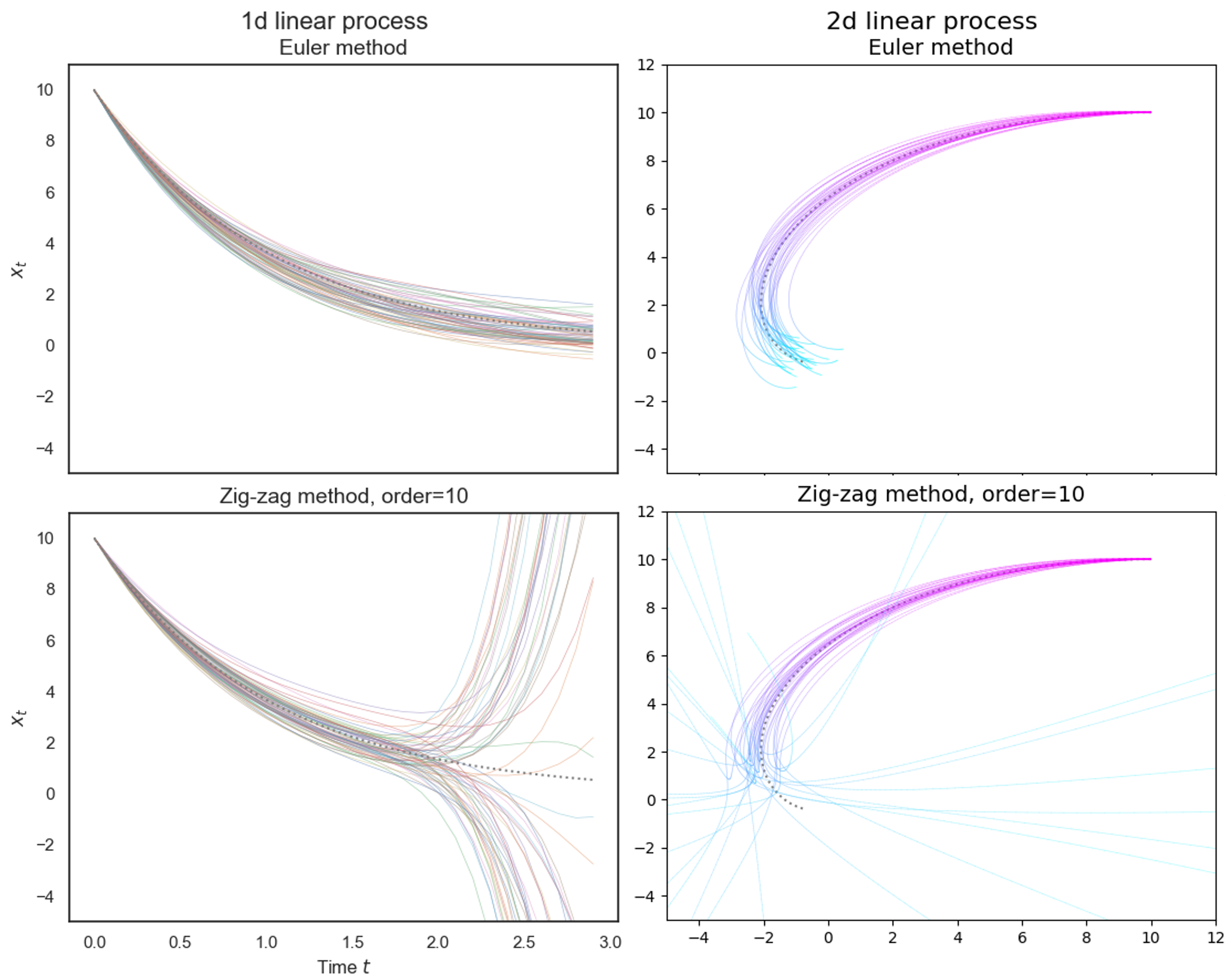
Figure 3.1: Numerical integration of 1 and 2 dimensional linear SDEs. On the left (resp. right) panels, we simulate a one (resp. two) dimensional linear SDE driven by a stationary Gaussian process with Gaussian autocovariance (white noise convolved with a Gaussian). For the top panels, we sampled white noise paths, convolved them with a Gaussian, and numerically integrated the resulting SDE pathwise using Euler’s method, providing a ’ground truth’ comparative baseline. For the bottom panels, we used the zigzag numerical integration method (both zigzag methods coincide for this system), plotting an exact Taylor expansion of solution sample paths that uses derivatives up to order $10$. On the left, each (1d) sample path is represented as a function of time in a different colour, while on the right each (2d) sample path is plotted on a plane with a start in magenta and an end in cyan. The path of least action (i.e. in the absence of noise) is plotted in each panel in a dotted grey line. Note that the trajectories in the top and bottom panels cannot be compared individually—only statistically—since they correspond to distinct noise realisations (since the noise samples are generated differently in each method).

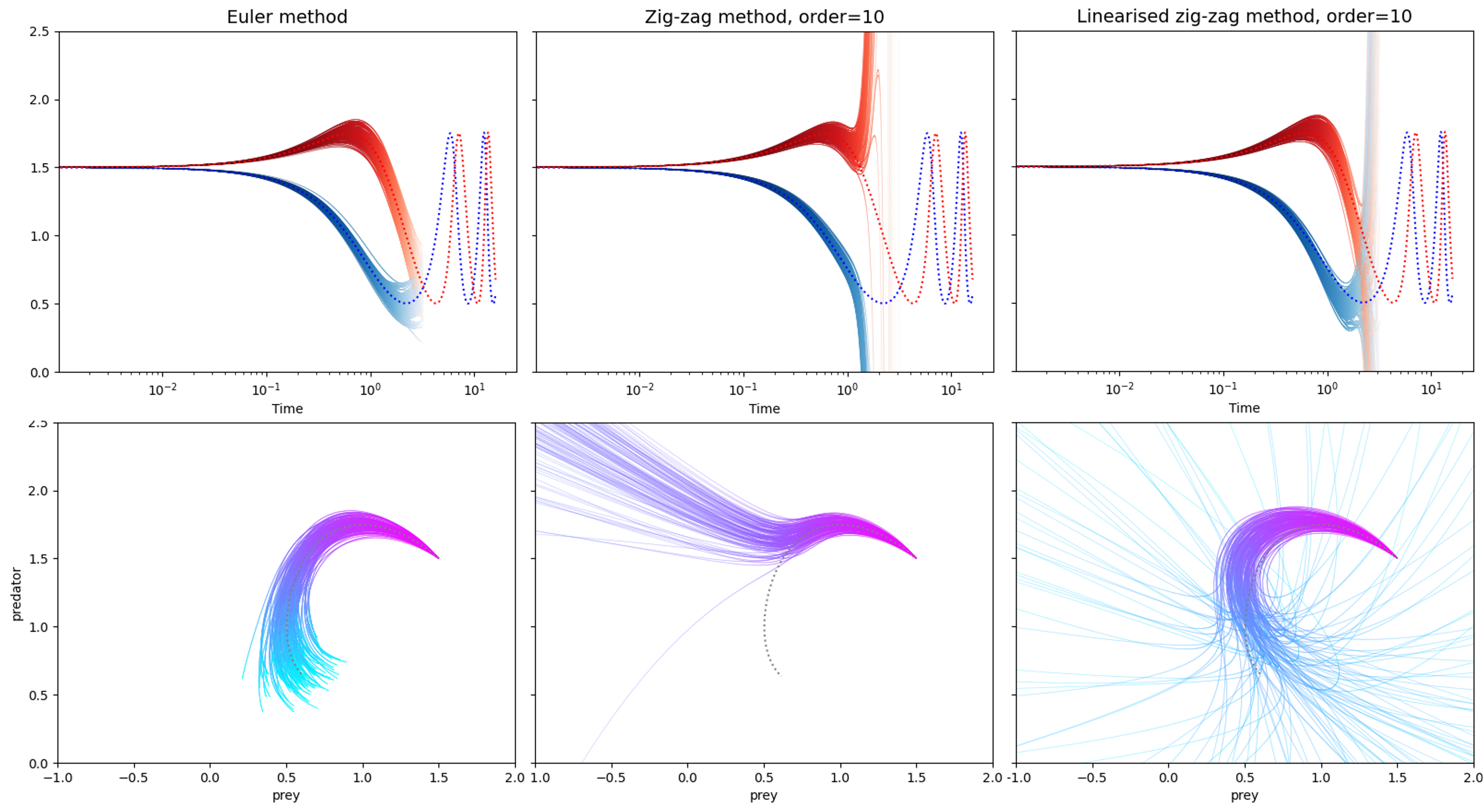
Figure 3.2: Numerical integration of stochastic Lotka-Volterra system. We simulate a stochastic Lotka-Volterra system driven by a stationary Gaussian process with Gaussian autocovariance (white noise convolved with a Gaussian). The Lotka-Volterra system is a toy model for the relative proportions of predator and prey in an ecosystem [63]. In the top panels we plot sample trajectories of the system over time, with the relative proportions of predators in red and prey in blue; in the bottom panels we plot these trajectories on a plane with a start in magenta and an end in cyan. The path of least action (i.e. in the absence of noise) is plotted in each panel as a dotted line. In the first column, we plot trajectories generated with Euler’s method, providing a ’ground truth’ comparative baseline. In the second and third columns, we plot trajectories generated with the zigzag and linearised zigzag methods. The zigzag and linearised zigzag methods solved the system for the same set of noise sample paths, while Euler’s method used a different set of noise samples (since the noise is realised differently in this method).

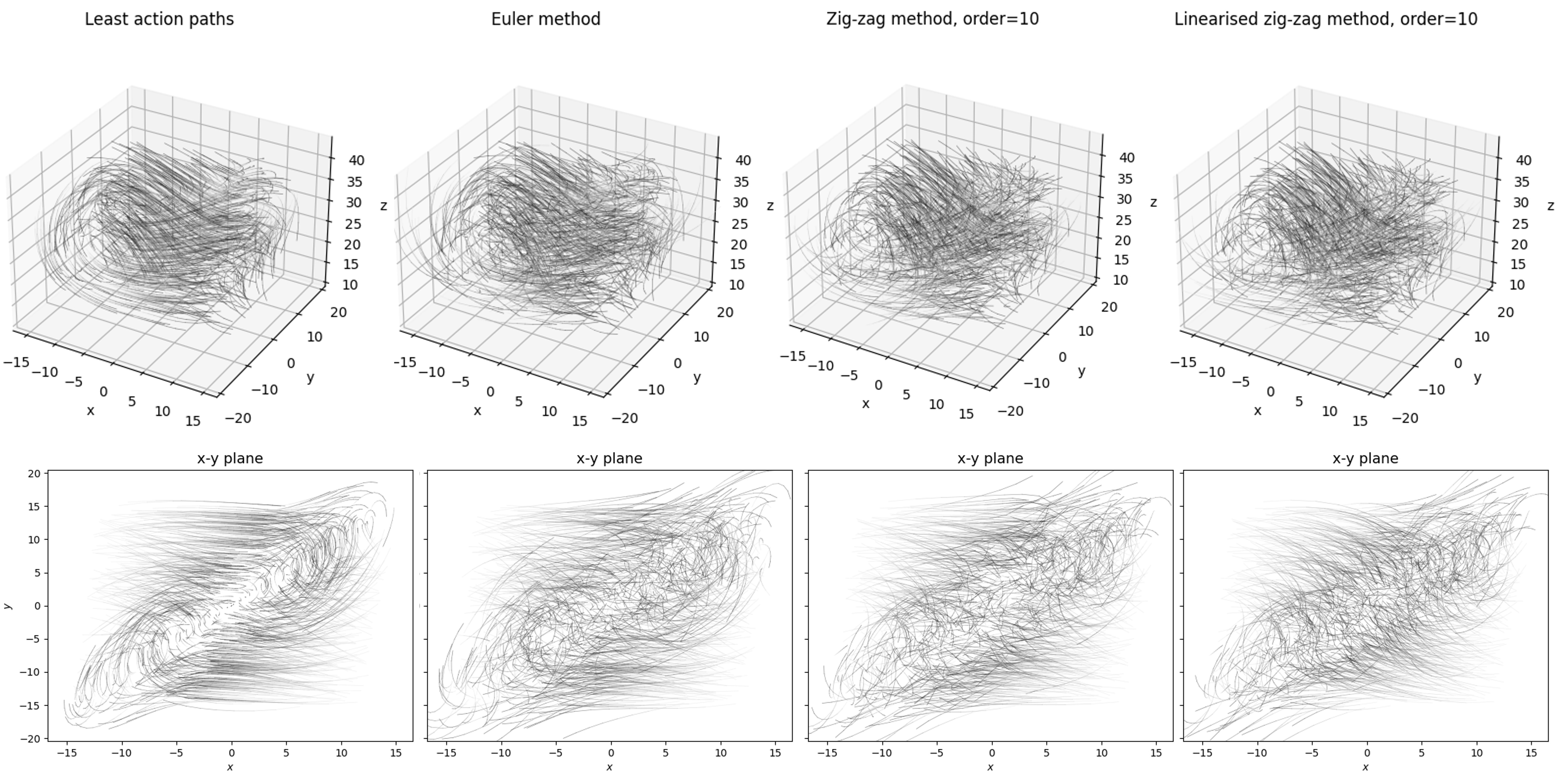
Figure 3.3: Numerical integration of stochastic Lorenz system. We simulate a stochastic Lorenz system driven by a stationary Gaussian process with Gaussian autocovariance (white noise convolved with a Gaussian). The plots are sample trajectories at various initialisations (shared across panels), in 3d in the top panels, with their 2d projections on the $x$-$y$ plane in the bottom panels. The first column shows paths of least action (i.e. in the absence of noise). The subsequent columns shows paths integrated with Euler, zigzag and linearised zigzag methods, respectively, where Euler serves as a comparative baseline. Importantly, the noise realisations were shared only by the zigzag and linearised zigzag methods (since the noise is realised differently in Euler’s method).

We compare integration methods on four simple SDEs driven by a stationary Gaussian process with Gaussian autocovariance. This choice of noise has two advantages: first, it is the canonical example of smooth noise; second it is perhaps the only example of coloured noise for which SDEs can be straightforwardly integrated using standard methods, providing a ’ground truth’ comparative baseline. Indeed, this is because this noise can alternatively be simulated by sampling white noise and convolving with a Gaussian, following which one can integrate the resulting SDE pathwise using Euler’s method (or any other established ODE solver). The systems we simulate are: one dimensional and two dimensional linear SDEs, see Figure 3.1; a stochastic Lotka-Volterra system, see Figure 3.2; and a stochastic Lorenz system, see Figure 3.3. For each system, we compare the zigzag methods with the baseline provided by Euler’s method.

3.1.3 Results

As expected, the (non-linearised) zigzag method provides extremely accurate trajectories on short time-spans—in virtue of Taylor’s theorem—until Taylor expansions blow up. The length of this timespan is somewhat inversely related with the amount of non-linearity of the underlying system. The surprising finding is that the linearised zigzag method yields trajectories that are almost as accurate and that remain accurate on a longer timespan; in addition to being computationally cheaper, the local linearised method appears to provide reconstructions that are more stable in time.

3.2 Most likely path via Lagrangian

Now we show a method that approximately recovers the most likely path of an SDE (1.1) from the finite order Lagrangian in generalised coordinates via a modified gradient descent. The ideas herein underlie the basis of (generalised) Bayesian filtering as presented in the next section, and have been used to relate the dynamics of multipartite processes to Bayesian filters in derivations of the free-energy principle [23, 24].

3.2.1 The method

The most likely path of the SDE (1.1), can be expressed as the unique solution to the ODE (2.38), which minimises the Lagrangian $\mathcal{L}$ at all times and for all orders $N$ (2.39). In contrast, the path of least action for finite order $N$, solutions to (2.36), generally leaves the constraint set where $\mathcal{L}$ is minimised.

Therefore, one would like to project the motion defining the path of least action (2.36) onto the constraint set, in order to approximate the most likely path of the SDE (1.1). One inexact yet simple way to do this is to subtract the gradient of the Lagrangian from its flow, so that the motion is always pulled back to the constraint set:

$$\dot{\bar{\mathbf{x}}}_{t}=\mathbf{D}\bar{\mathbf{x}}_{t}-\lambda\nabla\mathcal{L}(\bar{\mathbf{x}}_{t}).$$ (3.3)

and maintaining the initial condition (2.37). Here $\lambda>0$ is a weight; we chose this notation to be reminiscent of Lagrange multipliers. Intuitively, the solution to (3.3) should tend to the most likely path of (1.1) as $\lambda$ grows large.

3.2.2 Simulations and results

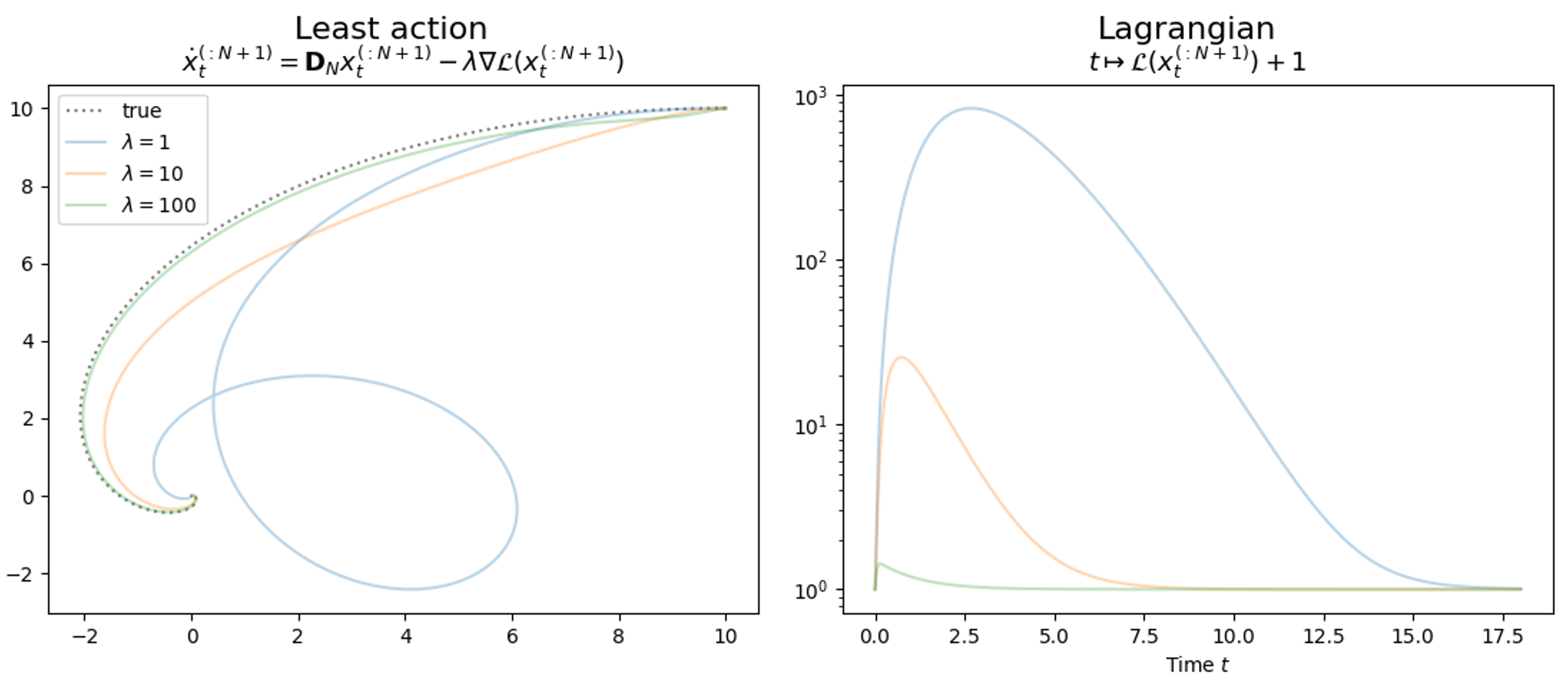
Figure 3.4: Recovering path of least action for linear SDE. Left: We show the true path of least action of a given 2 dimensional linear SDE with initial condition $(10,10)$ in a dashed grey line. We then show the solution to (3.3) for $N+1=4$ orders of motion and different weightings $\lambda=1,10,100$, confirming the claim that it tends to the path of least action as $\lambda$ grows large. Right: We plot the Lagrangian over time ($+1$ to plot in log-scale) for solutions to (3.3) corresponding to respective weightings of $\lambda$. The closer the solution is to the path of least action the more the Lagrangian is minimised at all times, and vice-versa.

We verify this claim on a simple simulation of a two dimensional linear SDE, where we numerically integrate (3.3) (with the initial condition (2.37)) using Euler’s method, for $N=4$ orders of motion, with several weightings of $\lambda>0$. The upshot is that indeed the solution to (3.3) tends to the most likely path of the SDE (1.1) as $\lambda$ grows large; please see Figure 3.4.

3.3 Bayesian filtering via generalised coordinates

The goal of generalised Bayesian filtering—like any filtering algorithm—is to infer latent variables from observations.

3.3.1 The simplest generative model

As a Bayesian method for filtering, we first specify a generative model. For didactic purposes, we consider a simple generative model and mention extensions in Section 3.3.6.

We assume that latent variables follow a stochastic differential equation, which constitutes the prior:

$$\frac{dx_{t}}{dt}=f\left(x_{t}\right)+w_{t},\quad x_{t}\in\mathbb{R}^{d}$$ (3.4)

where $w_{t}$ is an $\mathbb{R}^{d}$-valued stationary Gaussian process with $(N-1)$-times continuously differentiable sample paths a.s. and $f:\mathbb{R}^{d}\to\mathbb{R}^{d}$ is an $(N-1)$-times continuously differentiable vector field, and the initial condition for the SDE $x_{0}$ is distributed according to the Lebesgue measure. (The following can also be adapted to initial conditions following a probability distribution). In addition, we assume that observations are sampled as a function of latent variables plus some noise, which constitutes the likelihood

$$y_{t}=g\left(x_{t}\right)+z_{t},\quad y_{t}\in\mathbb{R}^{m}$$ (3.5)

where $g:\mathbb{R}^{d}\to\mathbb{R}^{m}$ is $M$-times continuously differentiable, and $z_{t}$ is an $\mathbb{R}^{m}$-valued stationary Gaussian process with $M$-times continuously differentiable sample paths a.s., and we take $M\leq N$ for later.

Reformulation in generalised coordinates

We reformulate the dynamics in generalised coordinates—this will simplify matters later. For the prior model we have, for all $t\in\mathbb{T}$,

$$\mathbf{D}^{\prime}\mathbf{x}_{t}=\mathbf{f}(\mathbf{x}_{t})+\mathbf{w}_{t},\quad\mathbf{w}_{t}\sim\mathcal{N}(0,\mathbf{\Sigma}^{w}),$$ (3.6)

with $\mathbf{D}^{\prime}\mathbf{x}_{t},\mathbf{w}_{t}$ random variables on $\mathbb{G}^{d,N-1}$, $\mathbf{x}_{t}$ on $\mathbb{G}^{d,N}$ and where $\mathbf{\Sigma}^{w}\in\operatorname{Mat}_{Nd,Nd}$ is given in terms of the autocovariance of $w$ as (2.7). As for the likelihood model

$$\mathbf{y}_{t}=\mathbf{g}(\mathbf{x}_{t})+\mathbf{z}_{t},\quad\mathbf{z}_{t}\sim\mathcal{N}(0,\mathbf{\Sigma}^{z}),$$ (3.7)

with $\mathbf{y}_{t},\mathbf{z}_{t}$ random variables on $\mathbb{G}^{d,M}$ and $\mathbf{\Sigma}^{z}\in\operatorname{Mat}_{(M+1)d,(M+1)d}$ is given in terms of the autocovariance of $z$ as (2.7), and the likelihood function in generalised coordinates $\mathbf{g}$ is obtained analogously to Definition 1.1.2. Specifically, the generalised likelihood is the function

$$\mathbf{g}:\mathbb{G}^{d,N}\to\mathbb{G}^{d,M},\mathbf{g}(\mathrm{z}^{(:N)})\triangleq\begin{pmatrix}\mathrm{g}^{(0)}(\mathrm{z}^{(0)})&\ldots&\mathrm{g}^{(M)}(\mathrm{z}^{(:M)})\end{pmatrix}^{\top}$$ (3.8)

where each component $\mathrm{g}^{(m)}:\mathbb{G}^{d,m}\to\mathbb{R}^{d}$ is defined implicitly through the relation

$$\mathrm{g}^{(m)}\left(x_{t},\frac{d}{dt}x_{t},\ldots,\frac{d^{m}}{dt^{m}}x_{t}\right)\triangleq\frac{d^{m}}{dt^{m}}g(x_{t}).$$ (3.9)

See (3.27) for the expression of $\mathbf{g}$ under the local linear approximation 1.1.3.

Altogether this furnishes a generative model under which we can do Bayesian inference:

$$\begin{split}p(\mathbf{y}_{t},\mathbf{x}_{t})&\triangleq p(\mathbf{y}_{t}\mid\mathbf{x}_{t})p(\mathbf{x}_{t})\\ p(\mathbf{y}_{t}\mid\mathbf{x}_{t})&=\mathcal{N}\left(\mathbf{y}_{t};\mathbf{g}(\mathbf{x}_{t}),\mathbf{\Sigma}^{z}\right)\\ \quad p(\mathbf{x}_{t})&=\mathcal{N}\left(\mathbf{D}^{\prime}\mathbf{x}_{t}-\mathbf{f}(\mathbf{x}_{t});0,\mathbf{\Sigma}^{w}\right).\end{split}$$ (3.10)

3.3.2 Approximate Bayesian inference under the Laplace approximation

We have the following Bayesian inference problem:

$$p(\mathbf{x}_{t}\mid\mathbf{y}_{t})=\frac{p(\mathbf{y}_{t}\mid\mathbf{x}_{t})p(\mathbf{x}_{t})}{p(\mathbf{y}_{t})}$$ (3.11)

Variational Bayesian inference

And we want to compute—or approximate—the posterior on the left. We do this through variational Bayesian inference [64, 65], where we approximate the posterior distribution with an approximate posterior distribution $q(\mathbf{x}_{t})$, by minimizing the following free energy functional:

$$\begin{split}\operatorname{F}(q;\mathbf{y}_{t})&\triangleq\mathbb{E}_{q}[\log q(\mathbf{x}_{t})-\log p(\mathbf{y}_{t},\mathbf{x}_{t})]\\ &=\underbrace{\mathbb{E}_{q}[-\log p(\mathbf{y}_{t},\mathbf{x}_{t})]}_{\text{Expected energy}}-\underbrace{\mathbb{E}_{q}[-\log q(\mathbf{x}_{t})]}_{\text{Entropy}}\\ &=\operatorname{D_{KL}}\left[q(\mathbf{x}_{t})\mid p(\mathbf{x}_{t}\mid\mathbf{y}_{t})\right]-\log p(\mathbf{y}_{t})\\ &\geq-\log p(\mathbf{y}_{t})\end{split}$$ (3.12)

In the penultimate line we can see that the free energy considered here is the KL divergence [66]—or relative entropy—between the approximate posterior and the true posterior, plus a constant. In other words, the free energy is minimized when and only when the approximate posterior equals the true posterior:

$$\delta_{q}\operatorname{F}(q;\mathbf{y}_{t})=0\iff q(\mathbf{x}_{t})=p(\mathbf{x}_{t}\mid\mathbf{y}_{t}).$$ (3.13)

The Laplace approximation

We are left with computing the free energy. The expected energy term in (3.12) is generally challenging to compute exactly and a standard approximation is the Laplace approximation [67, 68, 69]. In the Laplace approximation, we approximate the energy $V$

$$\begin{split}V(\mathbf{y}_{t},\mathbf{x}_{t})&\triangleq-\log p(\mathbf{y}_{t},\mathbf{x}_{t})\\ &\doteq\frac{1}{2}\left(\mathbf{y}_{t}-\mathbf{g}(\mathbf{x}_{t})\right)^{\top}(\mathbf{\Sigma}^{z})^{-1}\left(\mathbf{y}_{t}-\mathbf{g}(\mathbf{x}_{t})\right)+\frac{1}{2}\left(\mathbf{D}^{\prime}\mathbf{x}_{t}-\mathbf{f}(\mathbf{x}_{t})\right)^{\top}(\mathbf{\Sigma}^{w})^{-1}\left(\mathbf{D}^{\prime}\mathbf{x}_{t}-\mathbf{f}(\mathbf{x}_{t})\right)\end{split}$$ (3.14)

by a second order Taylor expansion at the mean of the approximate posterior $\bm{\mu}\triangleq\mu^{(:N)}\triangleq\mathbb{E}[q]$. From (3.10):

$$\begin{split}V(\mathbf{y}_{t},\mathbf{x}_{t})&\approx V(\mathbf{y}_{t},\bm{\mu})+\nabla_{\bm{\mu}}V(\mathbf{y}_{t},\bm{\mu})^{\top}\left(\mathbf{x}_{t}-\bm{\mu}\right)+\frac{1}{2}\left(\mathbf{x}_{t}-\bm{\mu}\right)^{\top}\nabla_{\bm{\mu}}^{2}V(\mathbf{y}_{t},\bm{\mu})\left(\mathbf{x}_{t}-\bm{\mu}\right).\end{split}$$ (3.15)

One can equivalently say that the Laplace approximation approximates the true posterior distribution by a Gaussian centered at $\bm{\mu}$. Indeed, by Bayes rule, the energy and the negative log posterior distribution are equal up to a constant, and the negative log posterior is quadratic if only if the posterior is Gaussian. Under the Laplace approximation we therefore choose our approximate posterior to also be Gaussian:

$$q(\mathbf{x}_{t};\bm{\mu},\mathbf{\Sigma})\triangleq\mathcal{N}(\mathbf{x}_{t};\bm{\mu},\mathbf{\Sigma})=\frac{1}{\sqrt{(2\pi)^{d(N+1)}\operatorname{det}(\mathbf{\Sigma})}}\exp\left(-\frac{1}{2}(\mathbf{x}_{t}-\bm{\mu})^{\top}\mathbf{\Sigma}^{-1}(\mathbf{x}_{t}-\bm{\mu})\right).$$ (3.16)

Under this parametric form, the free energy becomes a function of the parameters of the approximate posterior. The Laplace approximation is useful because the expected energy and entropy terms that form the free energy (3.12) become straightforward to evaluate:

$$\mathbb{E}_{q}[V(\mathbf{y}_{t},\mathbf{x}_{t})] \approx\mathbb{E}_{q}[V(\mathbf{y}_{t},\bm{\mu})]+\mathbb{E}_{q}[\nabla_{\bm{\mu}}V(\mathbf{y}_{t},\bm{\mu})^{\top}\left(\mathbf{x}_{t}-\bm{\mu}\right)]+\frac{1}{2}\mathbb{E}_{q}[\left(\mathbf{x}_{t}-\bm{\mu}\right)^{\top}\nabla_{\bm{\mu}}^{2}V(\mathbf{y}_{t},\bm{\mu})\left(\mathbf{x}_{t}-\bm{\mu}\right)]$$

$$=V(\mathbf{y}_{t},\bm{\mu})+\frac{1}{2}\operatorname{Tr}[\nabla_{\bm{\mu}}^{2}V(\mathbf{y}_{t},\bm{\mu})\mathbf{\Sigma}]$$ (3.17)

$$\mathbb{E}_{q}[-\log q(\mathbf{x}_{t};\bm{\mu},\mathbf{\Sigma})] =\frac{1}{2}\log\operatorname{det}\mathbf{\Sigma}+\frac{d(N+1)}{2}\log(2\pi\mathrm{e})$$ (3.18)

where the latter is the well-known entropy of a Gaussian distribution.

Consequently, we obtain a simple expression for the free energy under the Laplace approximation $\operatorname{F_{L}}$, by subtracting entropy (3.18) from the approximated expected energy (3.17), cf. (3.12):

$$\begin{split}\operatorname{F}(\bm{\mu},\mathbf{\Sigma};\mathbf{y}_{t})&\approx\operatorname{F_{L}}(\bm{\mu},\mathbf{\Sigma};\mathbf{y}_{t})\triangleq V(\mathbf{y}_{t},\bm{\mu})+\frac{1}{2}\operatorname{Tr}\left[\nabla_{\bm{\mu}}^{2}V(\mathbf{y}_{t},\bm{\mu})\mathbf{\Sigma}\right]-\frac{1}{2}\log\operatorname{det}\mathbf{\Sigma}-\frac{d(N+1)}{2}\log(2\pi\mathrm{e}).\end{split}$$ (3.19)

It remains to find the value of the parameters $\bm{\mu},\mathbf{\Sigma}$ that minimise the Laplace free energy, corresponding to the parameterisation of the approximate posterior that is closest to the true posterior.

Optimising the covariance

We can find the optimal covariance $\mathbf{\Sigma}^{*}$ by computing the free energy gradient (using Jacobi’s formula):

$$\begin{split}\nabla_{\mathbf{\Sigma}}\operatorname{F_{L}}(\bm{\mu},\mathbf{\Sigma};\mathbf{y}_{t})&=\frac{1}{2}\nabla_{\mathbf{\Sigma}}\operatorname{Tr}\left[\nabla_{\bm{\mu}}^{2}V(\mathbf{y}_{t},\bm{\mu})\mathbf{\Sigma}\right]-\frac{1}{2}\nabla_{\mathbf{\Sigma}}\log\operatorname{det}\mathbf{\Sigma}\\ &=\frac{1}{2}\nabla_{\bm{\mu}}^{2}V(\mathbf{y}_{t},\bm{\mu})-\frac{1}{2}\mathbf{\Sigma}^{-1}\\ \end{split}$$ (3.20)

and seeing when it vanishes:

$$\nabla_{\mathbf{\Sigma}}\operatorname{F_{L}}(\bm{\mu},\mathbf{\Sigma};\mathbf{y}_{t})=0\iff\mathbf{\Sigma}=\mathbf{\Sigma}^{*}(\mathbf{y}_{t},\bm{\mu})\triangleq\left(\nabla_{\bm{\mu}}^{2}V(\mathbf{y}_{t},\bm{\mu})\right)^{-1}.$$ (3.21)

It follows that the Laplace free energy evaluated at the optimal covariance reads as follows:

$$\begin{split}\operatorname{F_{L}}(\mu,\mathbf{\Sigma}^{*};\mathbf{y}_{t})&=V(\mathbf{y}_{t},\bm{\mu})+\frac{1}{2}\log\operatorname{det}\nabla_{\bm{\mu}}^{2}V(\mathbf{y}_{t},\bm{\mu})-\frac{d(N+1)}{2}\log(2\pi\mathrm{e}).\end{split}$$ (3.22)

Optimising the mean

The optimal mean $\bm{\mu}^{*}$ is that which minimises the Laplace free energy. Generalised filtering approaches this by a generalised gradient descent on Laplace free energy (3.22) (with $\lambda>0$; cf. Section 3.2.1):

$$\begin{split}\dot{\bm{\mu}}_{t}&=\mathbf{D}\bm{\mu}_{t}-\lambda\nabla_{\bm{\mu}}\operatorname{F_{L}}(\bm{\mu}_{t},\mathbf{\Sigma}^{*};\mathbf{y}_{t})\\ &=\mathbf{D}\bm{\mu}_{t}-\lambda\nabla_{\bm{\mu}}V(\mathbf{y}_{t},\bm{\mu}_{t})-\frac{\lambda}{2}\nabla_{\bm{\mu}}\log\operatorname{det}\nabla_{\bm{\mu}}^{2}V(\mathbf{y}_{t},\bm{\mu}_{t}).\end{split}$$ (3.23)

Here, the term $\nabla_{\bm{\mu}}V(\mathbf{y}_{t},\bm{\mu})$ can be interpreted as a weighted sum of generalised prediction errors (from (3.14)):

$$\begin{split}\nabla_{\bm{\mu}}V(\mathbf{y}_{t},{\bm{\mu}})&=(\nabla\mathbf{g}({\bm{\mu}}))^{\top}(\mathbf{\Sigma}^{z})^{-1}(\mathbf{g}({\bm{\mu}})-\mathbf{y}_{t})+(\mathbf{D}^{\prime}-\nabla\mathbf{f}({\bm{\mu}}))^{\top}(\mathbf{\Sigma}^{w})^{-1}(\mathbf{D}^{\prime}{\bm{\mu}}-\mathbf{f}({\bm{\mu}})).\end{split}$$ (3.24)

The latter term in the filtering dynamic (3.23) can be rewritten component-wise via Jacobi’s formula as

$$\partial_{\bm{\mu}_{i}}\log\operatorname{det}\nabla_{\bm{\mu}}^{2}V(\mathbf{y}_{t},\bm{\mu})=\operatorname{Tr}\left(\left(\nabla_{\bm{\mu}}^{2}V(\mathbf{y}_{t},\bm{\mu})\right)^{-1}\partial_{\bm{\mu}_{i}}\nabla_{\bm{\mu}}^{2}V(\mathbf{y}_{t},\bm{\mu})\right).$$ (3.25)

Therefore, generalised filtering (3.23) corresponds to a third order optimisation scheme on the energy $V(\mathbf{y}_{t},\bm{\mu})$.

Remark 3.3.1 (Domain of definition).

It is important to realise that the Laplace free energy (3.22) is defined for $\bm{\mu}$’s such that $\operatorname{det}\nabla_{\bm{\mu}}^{2}V(\mathbf{y}_{t},\bm{\mu})>0$, however, its gradient can be extended through (3.25) to the much wider region of $\bm{\mu}$’s such that $\operatorname{det}\nabla_{\bm{\mu}}^{2}V(\mathbf{y}_{t},\bm{\mu})\neq 0$, which makes the simulation of (3.23) straightforward. Of course, the solution to the generalised filtering equation (3.23) is continuous and cannot go from a region where $\operatorname{det}\nabla_{\bm{\mu}}^{2}V(\mathbf{y}_{t},\bm{\mu})<0$ to another where $\operatorname{det}\nabla_{\bm{\mu}}^{2}V(\mathbf{y}_{t},\bm{\mu})>0$ (in particular a neighbourhood of the free energy minimum) as in between lies a singularity with $\operatorname{det}\nabla_{\bm{\mu}}^{2}V(\mathbf{y}_{t},\bm{\mu})=0$ where the free energy gradient is not defined. But this issue becomes moot when numerically integrating (3.23) since discrete steps generally avoid these singularities. This makes it convenient for initialising (3.23) practically anywhere.

3.3.3 Summary of generalised filtering

In summary, generalised filtering dynamically updates a Gaussian approximate posterior belief $q$ over hidden variables $\mathbf{x}_{t}$ based on incoming data $\mathbf{y}_{t}$ and a generative model $p(\mathbf{y}_{t},\mathbf{x}_{t})$ (or its energy function $V=-\log p$) (3.10). The prescribed dynamics are as follows:

$$\begin{split}q(\mathbf{x}_{t};\bm{\mu}_{t},\mathbf{\Sigma}_{t})&\triangleq\mathcal{N}(\mathbf{x}_{t};\bm{\mu}_{t},\mathbf{\Sigma}_{t})\approx p(\mathbf{x}_{t}\mid\mathbf{y}_{t})\\ \dot{\bm{\mu}}_{t}&=\mathbf{D}\bm{\mu}_{t}-\lambda\nabla_{\bm{\mu}}V(\mathbf{y}_{t},\bm{\mu}_{t})-\frac{\lambda}{2}\nabla_{\bm{\mu}}\log\operatorname{det}\nabla_{\bm{\mu}}^{2}V(\mathbf{y}_{t},\bm{\mu}_{t})\\ \mathbf{\Sigma}_{t}&=\left(\nabla_{\bm{\mu}}^{2}V(\mathbf{y}_{t},\bm{\mu}_{t})\right)^{-1}\end{split}$$ (3.26)

where the initial condition $\bm{\mu}_{0}$ is arbitrary; $\lambda>0$ is a parameter measuring to what extent the solution is forced back to the free energy minimum; the gradient of the log determinant term has the closed form (3.25); and the generative model is given in generalised coordinates by (3.10). The second line of (3.26) can be seen as a third-order optimisation scheme; however, to the extent that the Laplace approximation (3.15) is valid, the final term in this line (3.26) is approximately zero and can often be neglected in practice. We will now see what such simplifications are afforded by the local linear approximation.

3.3.4 Simplifications under the local linear approximation

We now show how generalised filtering looks under the local linear approximation 1.1.3, which simplifies equations considerably. First of all, recall that the local linear approximation involves ignoring all derivatives of the flows $f,g$ of orders higher than one—that is, assuming that they vanish. We employ this assumption throughout this section.

Under the local linear approximation 1.1.3, the generalised flows read as:

$$\mathbf{f}(\mathbf{x}_{t})=\begin{pmatrix}f\left(\mathrm{x}_{t}^{(0)}\right)\\ \nabla f\left(\mathrm{x}_{t}^{(0)}\right)\mathrm{x}_{t}^{(1)}\\ \vdots\\ \nabla f\left(\mathrm{x}_{t}^{(0)}\right)\mathrm{x}_{t}^{(N)}\end{pmatrix},\quad\mathbf{g}(\mathbf{x}_{t})=\begin{pmatrix}g\left(\mathrm{x}_{t}^{(0)}\right)\\ \nabla g\left(\mathrm{x}_{t}^{(0)}\right)\mathrm{x}_{t}^{(1)}\\ \vdots\\ \nabla g\left(\mathrm{x}_{t}^{(0)}\right)\mathrm{x}_{t}^{(M)}\end{pmatrix}$$ (3.27)

The gradient of the energy (3.24) has the same functional form, but the Jacobians of the generalised flows within are given by considerably simpler expressions:

$$\begin{split}\underbrace{\nabla\mathbf{f}({\bm{\mu}})}_{\operatorname{Mat}_{d(N+1),d(N+1)}}=\underbrace{\nabla f(\mu^{(0)})}_{\operatorname{Mat}_{d,d}}\otimes\operatorname{I}_{N+1},\>\underbrace{\nabla\mathbf{g}({\bm{\mu}})}_{\operatorname{Mat}_{m(M+1),d(N+1)}}&=\underbrace{\nabla g(\mu^{(0)})}_{\operatorname{Mat}_{m,d}}\otimes\underbrace{\begin{pmatrix}1&&&&\overbrace{0}^{\operatorname{Mat}_{M+1,N-M}}\\ &1&&&0\\ &&\ddots&&\vdots\\ &&&1&0\end{pmatrix}}_{\operatorname{Mat}_{M+1,N+1}}\end{split}$$ (3.28)

The Hessian of the energy has a simpler form:

$$\begin{split}\nabla_{\bm{\mu}}^{2}V(\mathbf{y}_{t},\bm{\mu})&=(\nabla\mathbf{g}({\bm{\mu}}))^{\top}(\mathbf{\Sigma}^{z})^{-1}\nabla\mathbf{g}({\bm{\mu}})+(\mathbf{D}^{\prime}-\nabla\mathbf{f}({\bm{\mu}}))^{\top}(\mathbf{\Sigma}^{w})^{-1}(\mathbf{D}^{\prime}-\nabla\mathbf{f}({\bm{\mu}}))\end{split}$$ (3.29)

The coefficients of this Hessian are affine linear combinations of products of first order derivatives of the flows $f,g$. Consequently all third order derivatives of the energy vanish:

$$\nabla_{\bm{\mu}}^{3}V(\mathbf{y}_{t},{\bm{\mu}})\equiv 0.$$ (3.30)

This means that the the local linear approximation 1.1.3 implies the Laplace approximation (3.15):

$$\operatorname{F}=\operatorname{F_{L}}.$$ (3.31)

The optimal covariance $\mathbf{\Sigma}^{*}$ is given as the inverse of (3.29), cf. (3.21). And finally, the free energy gradient—evaluated at $\mathbf{\Sigma}^{*}$—is just the energy gradient:

$$\nabla_{\bm{\mu}}\operatorname{F_{L}}(\bm{\mu},\mathbf{\Sigma}^{*};\mathbf{y}_{t})=\nabla_{\bm{\mu}}V(\mathbf{y}_{t},\bm{\mu})$$ (3.32)

This is because the gradient of the log determinant term in the free energy (3.22) is a third order derivative of the energy (3.25), which vanishes under the local linear approximation by (3.30).

3.3.5 Summary of local linearised generalised filtering

In summary, generalised filtering under the local linear approximation 1.1.3 optimises a Gaussian approximate posterior belief $q$ over hidden variables $\mathbf{x}_{t}$ based on incoming data $\mathbf{y}_{t}$ and a generative model $p(\mathbf{y}_{t},\mathbf{x}_{t})$ (or energy function $V=-\log p$) (3.10) with flows $\mathbf{f},\mathbf{g}$ (3.27). The dynamics are as follows:

$$\begin{split}q(\mathbf{x}_{t};\bm{\mu}_{t},\mathbf{\Sigma}_{t})&\triangleq\mathcal{N}(\mathbf{x}_{t};\bm{\mu}_{t},\mathbf{\Sigma}_{t})\approx p(\mathbf{x}_{t}\mid\mathbf{y}_{t})\\ \dot{\bm{\mu}}_{t}&=\mathbf{D}\bm{\mu}_{t}-\lambda\nabla_{\bm{\mu}}V(\mathbf{y}_{t},\bm{\mu}_{t})\\ \mathbf{\Sigma}_{t}&=\left(\nabla_{\bm{\mu}}^{2}V(\mathbf{y}_{t},\bm{\mu}_{t})\right)^{-1}\end{split}$$ (3.33)

where the initial condition $\bm{\mu}_{0}$ is arbitrary; $\lambda>0$ is a parameter measuring to what extent the solution is forced back to the free energy minimum; the gradient and Hessian of the energy $V$ are given by (3.24) and (3.29), with the Jacobians of the generalised flows $\nabla\mathbf{f},\nabla\mathbf{g}$ within given by (3.28).

3.3.6 Practical and state-of-the-art implementation

There are several choices that underlie any practical implementation of generalised filtering (3.26), (3.33).

Numerical integration scheme

Perhaps the most important implementation choice is the numerical integrator for the dynamics of the (generalised) mean $\bm{\mu}$ in (3.26), (3.33). This dynamics is usually stiff; when the model’s flow $f$ and likelihood function $g$ are both linear, the Euler integrator might yield satisfactory integration, but with a small integration step, however, in the presence of any non-linearities the equation requires a more accurate solver with an adaptive step-size; here two choices are the Runge–Kutta–Fehlberg [70] and the more accurate albeit more expensive Ozaki solver [71, 17].

Data embedding in generalised coordinates

The generalised filtering schemes (3.26), (3.33) use a time-series of observations in generalised coordinates $t\mapsto\mathbf{y}_{t}$ up to some order $M$ ($0\leq M\leq N$) as input. However, it is often the case that we do not possess the higher order motion of our observations, that is as we operate in the absence of sensors for the velocity, acceleration, or higher orders of motion of our observations. In that case, one may want to obtain the higher orders of motion of observations from zero-th (or lower) order motion numerically.

The most basic way of recovering the higher orders of motion of zero-th order data is through finite differences, by setting

$$\begin{split}\mathrm{y}^{(1)}_{t}&\leftarrow\frac{\mathrm{y}^{(0)}_{t}-\mathrm{y}^{(0)}_{t-dt}}{dt},\quad\ldots\quad\mathrm{y}^{(M)}_{t}\leftarrow\frac{\mathrm{y}^{(M-1)}_{t}-\mathrm{y}^{(M-1)}_{t-dt}}{dt}\end{split}$$ (3.34)

where $dt$ is the length of the time interval between each observation (i.e. the sampling rate).

The more sophisticated way of obtaining the higher orders of motion of observations is by inverting a Taylor expansion. Since generalised coordinates are based on Taylor expansions, this is most compatible—and hence expected to work better—with generalised filtering. The Taylor polynomial associated with the (as yet unknown) generalised coordinate vector $\mathbf{y}_{t}$ is a polynomial of order $M$, which can be taken to fit $(M+1)$ points exactly. Take these points to be the known vectors $(\mathrm{y}^{(0)}_{t},\mathrm{y}^{(0)}_{t-dt},\ldots,\mathrm{y}^{(0)}_{t-Mdt})$ and $\mathbf{y}_{t}$ is uniquely determined. Explicitly, this is solving the following system of linear equations:

$$\mathrm{y}^{(0)}_{t-idt}=\sum_{n=0}^{M}\mathrm{y}^{(n)}_{t}\frac{(-idt)^{n}}{n!},\quad\forall i=0,1,\ldots,M$$ (3.35)

for the unknowns $\mathrm{y}^{(1)}_{t},\ldots,\mathrm{y}^{(M)}_{t}$. This is straightforward by inverting the matrix of Taylor coefficients.

Sampling rate of observations

In practice, the length of the time interval between each data point $dt$ can also be chosen (at the very least by down-sampling the time-series). This sampling rate needs to be chosen such that consecutive observations are most informative of the autocovariance of the data process. If the sampling rate is too small, consecutive data will be very smooth; and conversely if the sampling rate is too large, consecutive data will be very rough. One usually sets the sampling rate to correspond the intrinsic time-scale of the process, which can be taken to be the first zero-th crossing of the autocovariance of the observed time series.

Choosing the order

To select the order for generalised coordinates, one can leverage Taken’s embedding theorem. In short, the representation of a univariate time series through its successive derivatives up to order $2d$ is an embedding for an attractor of dimension $d$ [72, Th. 3]. Thus, the embedding order should be at most $2d$, that is, twice the dimension of the system. In practice, a lower embedding order might be sufficient to achieve a satisfying reconstruction accuracy. This can be determined by plotting the free-energy (over time) against the embedding order, and selecting the order that optimises the free-energy (through time). This yields the order with that best trades off accuracy of the filtered trajectory with model complexity. Indeed, this approach is recommended for selecting most hyperparameters, as discussed next.

Optimising choices of implementation

One straightforward way of optimising the method’s hyperparameters is by choosing them such that the (time integral of) free energy is minimised. This is because the free energy (3.12) can be rewritten as complexity minus accuracy:

$$\begin{split}\operatorname{F}(q;\mathbf{y}_{t})&=\underbrace{\operatorname{D_{KL}}[q(\mathbf{x}_{t})\mid p(\mathbf{x}_{t})]}_{\text{Complexity}}-\underbrace{\mathbb{E}_{q}[-\log p(\mathbf{y}_{t}\mid\mathbf{x}_{t})]}_{\text{Accuracy}}.\end{split}$$ (3.36)

Maximising accuracy entails finding explanations $q$ for the data that are maximally accurate explanations (i.e. maximum likelihood), while minimising complexity ensures that these explanations are as simple as possible above and beyond the prior (cf. Occam’s razor). In other words, the free energy (3.12) scores the extent to which our generative model and the parameters of the simulation produce good explanations for the data. Optimising the generative model and the parameters of the simulation to minimise (the time integral of) free energy is an instance of Bayesian model selection (cf. Bayes factor) [73]. Of course, doing this with successful results with the Laplace approximated free energy assumes that the Laplace approximation is a good approximation given the generative model at hand.

Extensions

Here we have presented generalised filtering in its simplest form, with a focus on mathematical clarity, but there are many ways in which this has been extended. Perhaps most important are parameter inference of the functions $f,g$ and fluctuations $w,z$ (i.e. their generalised covariance $\mathbf{\Sigma}^{w},\mathbf{\Sigma}^{z}$), and extensions to hierarchical generative models which include processes that evolve at multiple timescales of fast and slow (i.e. multi-scale processes [40]).

State-of-the-art implementation

The state-of-the-art implementation of generalised filtering can be found in the SPM academic software under the script DEM.m freely available here https://www.fil.ion.ucl.ac.uk/spm/software/. This has been optimised for nearly two decades for numerical stability by the neuroimaging community. (We will recapitulate implementations, which include versions in Python, in the software note, see Section 4.2. In this implementation, the method for numerical integration of generalised filtering is the Ozaki solver [71, 17], the method for embedding data into generalised coordinates is (3.35), and the order of motion for the data $M$ is always chosen to be equal to the order of motion for the latent states $N$. This implementation always uses the local linear approximation in generalised filtering, but has not been bench-marked against the non-linearised version—this could be the subject of future work. Nevertheless, there is a reason why the local linear approximation makes sense in the context of generalised filtering with the Laplace approximation. Discarding all derivatives of the flow, of order higher than one, has the advantage of making the functional form of the energy (3.14) nearly quadratic, which licenses the Laplace approximation. Conversely, dispensing with the local linear approximation can make the Laplace approximation a poor approximation (especially when $f,g$ are highly non-linear) hindering the method’s performance.

3.3.7 Simulations and results

We show the results of a simple simulation of generalised filtering on a partially observed stochastic Lorenz system. Despite its small-scale, this is a relatively challenging filtering problem because the stochastic Lorenz system exhibits stochastic chaos [74, 75, 76].

The generative process: The latent state of the data generating process $x_{t}$ is three dimensional and evolves according to a stochastic Lorenz system driven by a stationary Gaussian process with Gaussian autocovariance $w_{t}$ (i.e. white noise convolved with a Gaussian). The data we observe $y_{t}$ is one-dimensional and a noisy version of the sum of the latent states $x_{t}$ along each dimension, where the observation noise $z_{t}$ is a (one-dimensional) stationary Gaussian process with Gaussian autocovariance.

The generative model: For ease of exposition we take the generative model to be same as the generative process.

Simulation: We show the result of generalised filtering for different magnitudes of observation noise (i.e. noise volatility), in a regime with low observation noise (Figure 3.5, left) and another with high observation noise (Figure 3.5, right) using the state-of-the-art implementation detailed in Section 3.3.6, using $N=M=6$ orders of motion (twice the dimension of the Lorenz attractor, see 3.3.6). Please see Figure 3.5 for an illustration of real and inferred states as well as their difference measured in phase-space Euclidean distance

Results: The generalised filter is able to infer the latent state and reconstruct the attractor; in the regime of low observation noise the reconstruction is very accurate, while in the regime of high observation noise the reconstruction is accurate overall but misses many details, however this is to be expected given the low signal to noise ratio in this case.

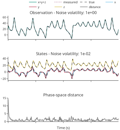
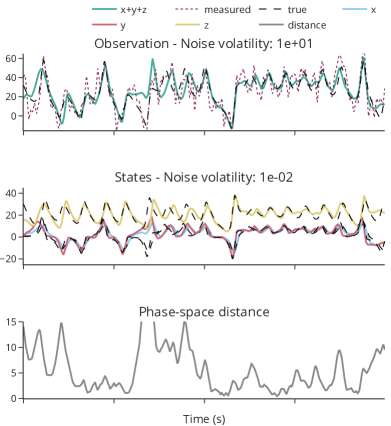
Figure 3.5: Generalised filtering for the Lorenz system. This Figure illustrates a simulation of generalised filtering on a partially observed stochastic Lorenz system, in a regime of low and high observation noise (left and right panel respectively). In the top panels, we see the one-dimensional time-series of noiseless observations in dashed black, corresponding to the sum of the three latent states. The data that were fed to the generalised filter comprised the measured time-series in dashed purple—this is the dashed black time-series plus observation noise. In the middle panels, there are three dashed black time-series corresponding to the latent states, which evolve according to a stochastic Lorenz system. In colour (yellow, red, blue) are the filtered time-series; that is, the most likely latent states at each time according to the approximate posterior belief $q$. In the top panel, the cyan time-series are filtered observation time-series, obtained as the sum of the coloured time-series in the middle panels. The bottom panel scores the Euclidean distance between filtered time-series in latent space and true time-series.

Discussion: This simulation has the limitation of using a generative model that is equal to the generative process which is unrealistic in practice. This was chosen to be as informative as possible to visualise the performance of the method. For more realistic high-dimensional simulations in real world scenarios we refer to [20, 21, 22].

Chapter 4:  Concluding remarks

4.1 Future directions

There are many directions that could attend future work:

Contextualisation within the literature: From a global perspective, we need a more comprehensive understanding of the convergence and differences between the theory of generalised coordinates and established approaches to the analysis and numerical treatment of stochastic differential equations with general classes of noise; for instance the relationship with standard stochastic analysis [5], rough path theory [7, 6], and the current theory of Markovian realisation [8, 9, 10].

Generalising theoretical results: From a technical perspective, many of the technical assumptions used throughout this work could be loosened and results generalised. For instance, one can presumably extend this theory to include equations with multiplicative noise, and use a similar local linearisation procedure for the noise to control the number of terms in the generalised coordinates expansion for analysis and numerics. Another important extension would be to multi-scale SDEs [40]. Additionally, it should be straightforward to generalise the theory to accommodate non-stationary Gaussian process noise.

Example 4.1.1.

For example, it would be nice to be able to work with noise of the form $w_{t}=\sum_{i=1}^{m}\xi_{i}\cos\left(\lambda_{i}t\right),t\in\mathbb{R},$ where $\xi_{1},\ldots,\xi_{m}$ are i.i.d. standard normal random variables and $\lambda_{1},\ldots,\lambda_{m}\geq 0$ are a finite set of frequencies. This process is a mean-zero, non-stationary Gaussian process with analytic sample paths. Random Fourier series of this form arise naturally from the Karhunen-Loéve expansion [4, Sec. 1.4].

[79, Theorem 4 and Corollary 1, p224-225] in combination with our Lemma 2.1.1 could be used to obtain the autocovariance of the generalised non-stationary process, and hence extend the whole construction. Lastly, the theory herein extends to arbitrary stochastic initial conditions, and the numerical integration methods to stochastic initial conditions that can be sampled from.

Extending analysis: There is potential to extend the analysis of the linear SDE in generalised coordinates to that of the local linearised SDE. In addition, it would be important to derive accuracy estimates for the local linearised version of an SDE compared to its non-linearised version (in generalised coordinates). Taken together this would yield an approximate analytic solution to any SDE with analytic flow and sample paths, and, by the Wong-Zakai theorems, to fairly arbitrary SDEs.

Accurate numerical simulation globally in time: Numerical integration with generalised coordinates is accurate on short time intervals, while the established techniques for numerical integration of processes driven by coloured noise (i.e. approximation with a diffusion process on a larger state-space followed by standard numerical schemes) is only accurate on longer timescales. This begs the question as to whether these two approaches could be combined in a multi-scale numerical simulation scheme, wherein integration steps of the latter method are interpolated with the former, yielding more accurate integration on all time scales.

Refining generalised filtering implementations: The theoretical foundation and derivation of generalised filtering presented in this paper shows the underlying assumptions and possible choices of implementation, such as committing to local linearisation versus non-linearisation. We hope that this treatment will help practitioners to refine existing—and devise improved—implementations. Practically, an intriguing project would be a comprehensive bench-marking of local linearised versus non-linearised generalised filtering. Another would be extending non-linearised generalised filtering to inferring parameters of the generative model—and to hierarchical generative models.

Stochastic control via generalised coordinates: Perhaps the largest omission from this paper are the established methods for stochastic control via generalised coordinates, developed in the area of continuous active inference [80, 81]. Briefly, just as generalised filtering operates by minimising the quantity known as free energy, active inference includes an additional control variable in the generative model—the actions—which are optimised to minimise free energy as well. In other words, free energy becomes a unified objective for action and perception. Continuous active inference generalises many existing algorithms to control, such as PID control [82], and may offer more robust and capable alternatives [83, 84]. Continuous active inference can also be combined with discrete active inference [85, 81] in continuous-discrete hierarchical generative models that can model human-level control [86, 87]. We expect that a detailed treatment of continuous active inference building upon—and at a similar level of detail—as the treatment of generalised filtering herein (with, possibly, its integration with discrete active inference) could fuel theoretical and algorithmic advances in state-of-the-art control.

4.2 Conclusion

In this paper, we presented a theory for the analysis, numerical simulation, and filtering of stochastic differential equations with many times differentiable flows and fluctuations. This translates the problem of analysing trajectories of SDEs into the simpler problem of finding the higher order motion of the solution (velocity, acceleration, jerk etc) and recovering the trajectories as Taylor expansions or Taylor series. By the Wong-Zakai approximation theorems this can be used to analyse a wide range of stochastic differential equation driven a wide range of noise signals, which may or may not be Markovian.

The conclusion is that SDEs with analytic flows and fluctuations are the SDE analogs to analytic functions. Like analytic functions, they can be usefully expressed and studied by their Taylor series; analogously to analytic functions, they can uniformly approximate the solutions to rougher, continuous SDEs on finite time-intervals, where the Wong-Zakai theorems take the place of the Weierstrass approximation theorem. The computational amenability of Taylor expansions enables computationally straightforward methods for numerical simulation, filtering and control. In this paper we formalised and developed these ideas, and argue that they have far-reaching implications throughout stochastic differential equations.

Software note

All simulations are reproducible with freely available code: for Sections 3.1 and 3.2 the code is available at https://github.com/lancelotdacosta/Generalised_coordinates; for Section 3.3, the simulations can be reproduced with https://colab.research.google.com/drive/1brsgc2gob-O_SjlgxyVg9R46VezIbP34?usp=sharing. At the time of writing, the state-of-the-art implementation of generalised filtering can be found in the SPM academic software under the script DEM.m freely available at https://www.fil.ion.ucl.ac.uk/spm/software/. We also draw attention to an implementation of generalised filtering in python available at https://github.com/johmedr/dempy.

Acknowledgements

The authors thank Mehran H. Bargzani and Philipp Hennig for interesting discussions that contributed to improving this paper.

Funding statement

LD is supported by the Fonds National de la Recherche, Luxembourg (Project code: 13568875). This publication is based on work partially supported by the EPSRC Centre for Doctoral Training in Mathematics of Random Systems: Analysis, Modelling and Simulation (EP/S023925/1). TP is supported by an NIHR Academic Clinical Fellowship (ref: ACF-2023-13-013). GP is partially supported by an ERC-EPSRC Frontier Research Guarantee through Grant No. EP/X038645, ERC Advanced Grant No. 247031 and a Leverhulme Trust Senior Research Fellowships, SRF$\backslash$R1$\backslash$241055.

Appendix A

A.1 Some frequently used notations

$\mathbb{T}$ time domain, open interval $\subset\mathbb{R}$, where usually we assume that $0\in\mathbb{T}$ (without loss of generality).

a.s. almost surely.

$\mathbb{G}^{d,n}$ the space of generalised coordinates (1.5).

$\mathbf{D},\mathbf{D}^{\prime}$ matrices in generalised coordinates (1.13).

$\mathbf{f}$ generalised flow, see Definition 1.1.2 (a vector field in generalised coordinates).

$\doteq$ equality up to an additive constant.

$\stackrel{{\scriptstyle\ell}}{{=}}$ equality in law, a.k.a. equality in distribution.

$\nabla,\nabla^{2}$ Jacobian and Hessian, e.g. $\nabla f:\mathbb{R}^{d}\to\mathbb{R}^{d\times d}$ is the Jacobian of $f$.

$L^{p}$ Lebesgue space.

$\operatorname{Mat}_{d,n}$ space of real-valued matrices with $d$ lines and $n$ columns.

A.2 A technical Lemma

This Lemma is useful for the analysis of the linear equation; specifically, for deriving Proposition 2.2.5:

Lemma A.2.1.

Suppose $(a_{n})_{n\geq 0}$, $(b_{n})_{n\geq 0}$ are sequences of non-negative real numbers such that $b_{n}=\max_{0\leq i\leq n}a_{i}$. Then

$$\limsup_{\begin{subarray}{c}n+m\to\infty\\ n,m\geq 1\end{subarray}}\left(\frac{a_{n+m}}{n!m!}\right)^{\frac{1}{n+m}}=\limsup_{\begin{subarray}{c}n+m\to\infty\\ n,m\geq 1\end{subarray}}\left(\frac{b_{n+m}}{n!m!}\right)^{\frac{1}{n+m}}.$$ (A.1)

Proof.

Without loss of generality we will show (A.1) along non-decreasing sequences of indices: let $(n_{k},m_{k})_{k\geq 0}$ be a sequence of tuples of natural numbers such that $n_{k}+m_{k}\to\infty$ and $(n_{k})_{k\geq 0}$, $(m_{k})_{k\geq 0}$ are non-decreasing. It suffices to show (A.1) along this sequence. Clearly, $0\leq\text{LHS}\leq\text{RHS}$ in (A.1).

First suppose $(a_{n})_{n\geq 0}$ is bounded by $c>0$. Then so is $(b_{n})_{n\geq 0}$. So by Stirling’s formula for the asymptotic of the factorial

$$\left(\frac{b_{n_{k}+m_{k}}}{n_{k}!m_{k}!}\right)^{\frac{1}{n_{k}+m_{k}}} \leq\left(\frac{c}{n_{k}!m_{k}!}\right)^{\frac{1}{n_{k}+m_{k}}}\sim\left(\frac{c2\pi e^{n_{k}+m_{k}}}{n_{k}^{n_{k}+1/2}m_{k}^{m_{k}+1/2}}\right)^{\frac{1}{n_{k}+m_{k}}}\xrightarrow{k\to\infty}0.$$

Thus in this case $\text{LHS}=\text{RHS}=0$ in (A.1).

Suppose now that $(a_{n})_{n\geq 0}$ is unbounded. We can then extract the infinite subsequences $(a_{n_{k_{j}}})_{j\geq 0}$, $(b_{n_{k_{j}}})_{j\geq 0}$ such that $a_{n_{k_{j}}}=b_{n_{k_{j}}}$ for all $j$. Since

$$\limsup_{j\to\infty}\left(\frac{a_{n_{k_{j}}+m_{k_{j}}}}{n_{k_{j}}!m_{k_{j}}!}\right)^{\frac{1}{n_{k_{j}}+m_{k_{j}}}} \leq\limsup_{k\to\infty}\left(\frac{a_{n_{k}+m_{k}}}{n_{k}!m_{k}!}\right)^{\frac{1}{n_{k}+m_{k}}}$$ (A.2)

$$\rotatebox{90.0}{$=\;\;$} \hskip 54.06006pt\rotatebox{90.0}{$\geq$}$$

$$\limsup_{j\to\infty}\left(\frac{b_{n_{k_{j}}+m_{k_{j}}}}{n_{k_{j}}!m_{k_{j}}!}\right)^{\frac{1}{n_{k_{j}}+m_{k_{j}}}} \leq\limsup_{k\to\infty}\left(\frac{b_{n_{k}+m_{k}}}{n_{k}!m_{k}!}\right)^{\frac{1}{n_{k}+m_{k}}}$$

it suffices to show the bottom inequality is an equality to show equality throughout. For this, it suffices to show that for $j$ large enough, if $b_{n_{k_{j}}+m_{k_{j}}}=b_{n_{k}+m_{k}}$ with $k\geq k_{j}$, then

$$\left(\frac{b_{n_{k_{j}}+m_{k_{j}}}}{n_{k_{j}}!m_{k_{j}}!}\right)^{\frac{1}{n_{k_{j}}+m_{k_{j}}}}\geq\left(\frac{b_{n_{k_{j}}+m_{k_{j}}}}{n_{k}!m_{k}!}\right)^{\frac{1}{n_{k}+m_{k}}}=\left(\frac{b_{n_{k}+m_{k}}}{n_{k}!m_{k}!}\right)^{\frac{1}{n_{k}+m_{k}}}.$$ (A.3)

For $c>0$, define the function $f_{c}:\mathbb{R}_{>0}^{2}\to\mathbb{R}_{>0}$ by

$$f_{c}(x,y)\triangleq\left(\frac{c}{\Gamma(x+1)\Gamma(y+1)}\right)^{\frac{1}{x+y}},$$

where $\Gamma$ is the gamma function. For (A.3) to hold for all $j$ large enough it suffices by the mean value theorem that there are $C,M>0$ such that for all $c\geq C$ and $x+y\geq M$ we have $\partial_{x}f_{c}(x,y),\partial_{y}f_{c}(x,y)\leq 0$.

We proceed to show this. We have

$$\partial_{x}f_{c}(x,y)=\bigg{(}-\frac{\psi(x+1)}{x+y}+\frac{-\log(c)+\log(\Gamma(x+1))+\log(\Gamma(y+1))}{(x+y)^{2}}\bigg{)}\left(\frac{c}{\Gamma(x+1)\Gamma(y+1)}\right)^{\frac{1}{x+y}}$$ (A.4)

and

$$\partial_{y}f_{c}(x,y)=\bigg{(}-\frac{\psi(y+1)}{x+y}+\frac{-\log(c)+\log(\Gamma(x+1))+\log(\Gamma(y+1))}{(x+y)^{2}}\bigg{)}\left(\frac{c}{\Gamma(x+1)\Gamma(y+1)}\right)^{\frac{1}{x+y}}$$ (A.5)

where $\psi\triangleq\Gamma^{\prime}/\Gamma$ is the digamma function. Note that $\psi(x+1)\geq\log(x)$ for all $x>0$, and $\log(\Gamma(x+1))=x\log(x)-x+o(x)$ as $x\to\infty$. From (A.4) we get for $x>0$

$$\partial_{x}f_{c}(x,y) \leq(-(x+y)\log(x)-\log(c)+x\log(x)-x+o(x)+y\log(y)-y+o(y))g_{c}(x,y)$$

$$=(-\log(c)-x-y+o(x+y))g_{c}(x,y)$$

for some positive function $g_{c}:\mathbb{R}^{2}_{>0}\to\mathbb{R}_{>0}$, where the error term $o(x+y)$ does not depend on $c$. Thus, fixing a $C>0$, we see that there is $M>0$ such that for all $c\geq C$ and $x+y\geq M$, $\partial_{x}f_{c}(x,y)\leq 0$. From (A.5) we the case of $\partial_{y}f_{c}$ is analoguous, which concludes the proof. ∎

References

- [1] K Kawasaki. Simple derivations of generalized linear and nonlinear Langevin equations. Journal of Physics A: Mathematical, Nuclear and General, 6(9):1289–1295, September 1973.
- [2] Luc Rey-Bellet. Open Classical Systems. In Stéphane Attal, Alain Joye, and Claude-Alain Pillet, editors, Open Quantum Systems II: The Markovian Approach, Lecture Notes in Mathematics, pages 41–78. Springer, Berlin, Heidelberg, 2006.
- [3] A. Einstein. Über die von der molekularkinetischen Theorie der Wärme geforderte Bewegung von in ruhenden Flüssigkeiten suspendierten Teilchen. Annalen der Physik, 322(8):549–560, 1905.
- [4] Grigorios A. Pavliotis. Stochastic Processes and Applications: Diffusion Processes, the Fokker-Planck and Langevin Equations. Number volume 60 in Texts in Applied Mathematics. Springer, New York, 2014.
- [5] Sheng-Wu He, Jia-Gang Wang, and Jia-an Yan. Semimartingale Theory and Stochastic Calculus. Routledge, Beijing, 1st edition edition, September 1992.
- [6] Peter K. Friz and Nicolas B. Victoir. Multidimensional Stochastic Processes as Rough Paths: Theory and Applications. Cambridge University Press, Cambridge, 1st edition edition, March 2010.
- [7] Peter K. Friz and Martin Hairer. A Course on Rough Paths: With an Introduction to Regularity Structures. Springer, 2nd edition edition, May 2020.
- [8] Anders Lindquist and Giorgio Picci. Linear Stochastic Systems: A Geometric Approach to Modeling, Estimation and Identification. Series in Contemporary Mathematics. Springer-Verlag, Berlin Heidelberg, 2015.
- [9] Sanjoy Mitter, Giorgio Picci, and Anders Lindquist. Toward a theory of nonlinear stochastic realization. In Feedback and Synthesis of Linear and Nonlinear Systems, 1981.
- [10] T. J. S. Tayor and M. Pavon. On the nonlinear stochastic realization problem. Stochastics and Stochastic Reports, 26(2):65–79, February 1989.
- [11] S. N. Gomes, G. A. Pavliotis, and U. Vaes. Mean Field Limits for Interacting Diffusions with Colored Noise: Phase Transitions and Spectral Numerical Methods. Multiscale Model. Simul., 18(3):1343–1370, 2020.
- [12] MH Duong and GA Pavliotis. Mean field limits for non-Markovian interacting particles: Convergence to equilibrium, generic formalism, asymptotic limits and phase transitions. Communications in Mathematical Sciences, 16:2199–2230, 2018.
- [13] P. Hanggi and P. Jung. Colored noise in dynamical systems. In Prigogine, I and Rice, SA, editor, Advances in Chemical Physics, VOL LXXXIX, volume 89 of Advances in Chemical Physics, pages 239–326. 1995.
- [14] G. A. Pavliotis, G. Stoltz, and U. Vaes. Scaling limits for the generalized Langevin equation. J. Nonlinear Sci., 31(1):Paper No. 8, 58, 2021.
- [15] M. Ottobre and G. A. Pavliotis. Asymptotic analysis for the generalized Langevin equation. Nonlinearity, 24(5):1629–1653, 2011.
- [16] R. L. Stratonovich. Topics in the Theory of Random Noise, Volume I. Martino Fine Books, July 2014.
- [17] K. J. Friston, N. Trujillo-Barreto, and J. Daunizeau. DEM: A variational treatment of dynamic systems. NeuroImage, 41(3):849–885, July 2008.
- [18] Karl Friston, Klaas Stephan, Baojuan Li, and Jean Daunizeau. Generalised Filtering. Mathematical Problems in Engineering, 2010:1–34, 2010.
- [19] Bhashyam Balaji and Karl Friston. Bayesian state estimation using generalized coordinates. In Ivan Kadar, editor, SPIE Defense, Security, and Sensing, page 80501Y, Orlando, Florida, United States, May 2011.
- [20] Fred Bos, Ajith Anil Meera, Dennis Benders, and Martijn Wisse. Free energy principle for state and input estimation of a quadcopter flying in wind. In 2022 International Conference on Robotics and Automation (ICRA), pages 5389–5395. IEEE, 2022.
- [21] Ajith Anil Meera and Pablo Lanillos. Adaptive noise covariance estimation under colored noise using dynamic expectation maximization. In 2023 62nd IEEE Conference on Decision and Control (CDC), pages 165–171. IEEE, 2023.
- [22] Ajith Anil Meera and Martijn Wisse. Dynamic expectation maximization algorithm for estimation of linear systems with colored noise. Entropy, 23(10):1306, 2021.
- [23] Karl Friston, Lancelot Da Costa, Noor Sajid, Conor Heins, Kai Ueltzhöffer, Grigorios A. Pavliotis, and Thomas Parr. The free energy principle made simpler but not too simple. Physics Reports, 1024:1–29, June 2023.
- [24] Karl Friston, Lancelot Da Costa, Dalton A. R. Sakthivadivel, Conor Heins, Grigorios A. Pavliotis, Maxwell Ramstead, and Thomas Parr. Path integrals, particular kinds, and strange things. Physics of Life Reviews, August 2023.
- [25] Garrett Birkhoff. Ordinary Differential Equations 4e. John Wiley & Sons, New York, 4e édition edition, January 1989.
- [26] Earl A. Coddington and Norman Levinson. Theory of differential equations. McGraw-Hill Education, New Delhi, March 1984.
- [27] CALCUL INTÉGRAL. – Mémoire sur l’emploi du calcul des limites dans l’intégration des équations aux dérivées partielles. In Augustin-Louis Cauchy, editor, Oeuvres Complètes: Series 1, volume 7 of Cambridge Library Collection - Mathematics, pages 17–33. Cambridge University Press, Cambridge, 2009.
- [28] Sophie von Kowalevsky. Zur Theorie der partiellen Differentialgleichung. Journal für die reine und angewandte Mathematik, 80:1–32, 1875.
- [29] Gerald Teschl. Ordinary Differential Equations and Dynamical Systems. Amer Mathematical Society, Providence, R.I, August 2012.
- [30] Lars Hörmander. The Analysis of Linear Partial Differential Operators I: Distribution Theory and Fourier Analysis. Springer, Berlin ; New York, 2nd ed. 2003 edition edition, October 2013.
- [31] Anonymous. Infinite sum of normals. https://math.stackexchange.com/questions/674128/infinite-sum-of-normals, 2014. Accessed: 2024-08-25.
- [32] Anonymous. Infinite sum of normal r.v. is still a normal r.v when given sum limits. https://math.stackexchange.com/questions/1110461/infinite-sum-of-normal-r-v-is-still-a-normal-r-v-when-given-sum-limits-i-1, 2014. Accessed: 2024-08-25.
- [33] Elias M. Stein and Rami Shakarchi. Complex Analysis. Princeton University Press, Princeton, N.J, illustrated edition edition, April 2003.
- [34] Uniform limit of holomorphic functions. https://math.stackexchange.com/questions/368664/uniform-limit-of-holomorphic-functions.
- [35] Yu. K. Belyaev. Local Properties of the Sample Functions of Stationary Gaussian Processes. Theory of Probability & Its Applications, 5(1):117–120, January 1960.
- [36] E. Wong and M. Zakai. On the convergence of ordinary integrals to stochastic integrals. Ann. Math. Statist., 36:1560–1564, 1965.
- [37] István Gyöngy and György Michaletzky. On Wong–Zakai approximations with –martingales. Proceedings of the Royal Society of London. Series A: Mathematical, Physical and Engineering Sciences, 460(2041):309–324, January 2004.
- [38] S. Watanabe and N. Ikeda. Stochastic Differential Equations and Diffusion Processes. North Holland, Amsterdam ; New York : Tokyo : New York, NY, 0 edition edition, February 1981.
- [39] S. Bo and A. Celani. White-noise limit of nonwhite nonequilibrium processes. Phys. Rev. E, 88:062150, Dec 2013.
- [40] Grigoris Pavliotis and Andrew Stuart. Multiscale Methods: Averaging and Homogenization. Springer, New York, NY, softcover reprint of hardcover 1st ed. 2008 édition edition, November 2010.
- [41] T. Diamantakis, D. D. Holm, and G. A. Pavliotis. Variational principles on geometric rough paths and the Lévy area correction. SIAM J. Appl. Dyn. Syst., 22(2):1182–1218, 2023.
- [42] Chengcheng Ling, Sebastian Riedel, and Michael Scheutzow. A Wong-Zakai theorem for SDEs with singular drift. Journal of Differential Equations, 326:344–363, July 2022.
- [43] Franz Konecny. On Wong-Zakai approximation of stochastic differential equations. Journal of Multivariate Analysis, 13(4):605–611, December 1983.
- [44] Laure Coutin and Antoine Lejay. Semi-martingales and rough paths theory. Electronic Journal of Probability, 10(none):761–785, January 2005.
- [45] Lauri Viitasaari and Caibin Zeng. Stationary Wong–Zakai Approximation of Fractional Brownian Motion and Stochastic Differential Equations with Noise Perturbations. Fractal and Fractional, 6(6):303, June 2022.
- [46] Ramiro Scorolli. Wong-Zakai approximations for quasilinear systems of It\^o’s type stochastic differential equations driven by fBm with $H1/2$, November 2021.
- [47] Laure Coutin and Zhongmin Qian. Stochastic analysis, rough path analysis and fractional Brownian motions. Probability Theory and Related Fields, 122(1):108–140, January 2002.
- [48] Richard F. Bass, Ben Hambly, and Terry J. Lyons. Extending the Wong-Zakai theorem to reversible Markov processes. Journal of the European Mathematical Society, 4(3):237–269, September 2002.
- [49] Peter Friz and Nicolas Victoir. On uniformly subelliptic operators and stochastic area. Probability Theory and Related Fields, 142(3-4):475–523, November 2008.
- [50] Antoine Lejay. Stochastic differential equations driven by processes generated by divergence form operators II: Convergence results. ESAIM: Probability and Statistics, 12:387–411, July 2008.
- [51] Peter Friz and Harald Oberhauser. Rough path limits of the Wong–Zakai type with a modified drift term. Journal of Functional Analysis, 256(10):3236–3256, May 2009.
- [52] Nathaël Da Costa, Marvin Pförtner, Lancelot Da Costa, and Philipp Hennig. Sample Path Regularity of Gaussian Processes from the Covariance Kernel, February 2024.
- [53] Michael Scheuerer. Regularity of the sample paths of a general second order random field. Stochastic Processes and their Applications, 120(10):1879–1897, September 2010.
- [54] Weak convergence of a sequence of gaussian random vector. https://math.stackexchange.com/questions/3625473/weak-convergence-of-a-sequence-of-gaussian-random-vector?noredirect=1&lq=1.
- [55] limit of gaussian process. https://math.stackexchange.com/questions/1358608/limit-of-gaussian-process.
- [56] Claude Godrèche and Jean-Marc Luck. Characterising the nonequilibrium stationary states of Ornstein-Uhlenbeck processes. Journal of Physics A: Mathematical and Theoretical, 52(3):035002, January 2019.
- [57] Olav Kallenberg. Foundations of Modern Probability. Springer, Cham, Switzerland, 3rd ed. 2021 edition edition, February 2021.
- [58] H. Risken. The Fokker-Planck Equation: Methods of Solution and Applications. Springer Series in Synergetics. Springer-Verlag, Berlin Heidelberg, 2 edition, 1996.
- [59] C. Soize. The Fokker-Planck equation for stochastic dynamical systems and its explicit steady state solutions, volume 17 of Series on Advances in Mathematics for Applied Sciences. World Scientific Publishing Co. Inc., River Edge, NJ, 1994.
- [60] Udo Seifert. Stochastic thermodynamics, fluctuation theorems and molecular machines. Reports on Progress in Physics, 75(12):126001, November 2012.
- [61] M. Chaichian and A. Demichev. Path Integrals in Physics: Volume I Stochastic Processes and Quantum Mechanics. CRC Press, Bristol, 1st edition edition, July 2001.
- [62] M. Chaichian and A. Demichev. Path Integrals in Physics: Volume II Quantum Field Theory, Statistical Physics and Other Modern Applications. CRC Press, Bristol, 1st edition edition, July 2001.
- [63] X. Mao, G. Marion, and E. Renshaw. Environmental Brownian noise suppresses explosions in population dynamics. Stochastic Process. Appl., 97(1):95–110, 2002.
- [64] David M. Blei, Alp Kucukelbir, and Jon D. McAuliffe. Variational Inference: A Review for Statisticians. Journal of the American Statistical Association, 112(518):859–877, April 2017.
- [65] Christopher M. Bishop. Pattern Recognition and Machine Learning. Information Science and Statistics. Springer, New York, 2006.
- [66] S. Kullback and R. A. Leibler. On Information and Sufficiency. The Annals of Mathematical Statistics, 22(1):79–86, March 1951.
- [67] David J. C. MacKay. Bayesian Interpolation. Neural Computation, 4(3):415–447, May 1992.
- [68] Karl Friston, Jérémie Mattout, Nelson Trujillo-Barreto, John Ashburner, and Will Penny. Variational free energy and the Laplace approximation. NeuroImage, 34(1):220–234, January 2007.
- [69] C.K.I. Williams and D. Barber. Bayesian classification with Gaussian processes. IEEE Transactions on Pattern Analysis and Machine Intelligence, 20(12):1342–1351, December 1998.
- [70] Ernst Hairer, Syvert P. Nørsett, and Gerhard Wanner. Solving Ordinary Differential Equations I: Nonstiff Problems. Springer Science & Business Media, April 2008.
- [71] Tohru Ozaki. A Bridge Between Nonlinear Time Series Models and Nonlinear Stochastic Dynamical Systems: A Local Linearization Approach. Statistica Sinica, 2(1):113–135, 1992.
- [72] Floris Takens. Detecting strange attractors in turbulence. Lecture Notes in Mathematics, Berlin Springer Verlag, 898:366, 1981.
- [73] José M. Bernardo and Adrian F. M. Smith. Bayesian Theory. John Wiley & Sons, September 2009.
- [74] Kody Law, Andrew Stuart, and Konstantinos Zygalakis. Data Assimilation: A Mathematical Introduction. Springer, Cham Heidelberg New York Dordrecht London, softcover reprint of the original 1st ed. 2015 édition edition, October 2016.
- [75] Sebastian Reich and Colin Cotter. Probabilistic Forecasting and Bayesian Data Assimilation. Cambridge University Press, Cambridge, 2015.
- [76] Karl Friston, Conor Heins, Kai Ueltzhöffer, Lancelot Da Costa, and Thomas Parr. Stochastic Chaos and Markov Blankets. Entropy, 23(9):1220, September 2021.
- [77] R. Kupferman, G. A. Pavliotis, and A. M. Stuart. Itô versus Stratonovich white-noise limits for systems with inertia and colored multiplicative noise. Phys. Rev. E (3), 70(3):036120, 9, 2004.
- [78] G Pesce, A McDaniel, S Hottovy, J Wehr, and G Volpe. Stratonovich-to-Itô transition in noisy systems with multiplicative feedback. Nat. Commun., 4:2733, 2013.
- [79] Iosif I. Gikhman and Anatoli V. Skorokhod. The Theory of Stochastic Processes I. Springer, Berlin ; New York, reprint of the 1st ed. berlin heidelberg new york 1974 edition edition, March 2004.
- [80] Karl J. Friston, Jean Daunizeau, James Kilner, and Stefan J. Kiebel. Action and behavior: A free-energy formulation. Biological Cybernetics, 102(3):227–260, March 2010.
- [81] Thomas Parr, Giovanni Pezzulo, and Karl J. Friston. Active Inference: The Free Energy Principle in Mind, Brain, and Behavior. MIT Press, Cambridge, MA, USA, March 2022.
- [82] Manuel Baltieri and Christopher L. Buckley. PID Control as a Process of Active Inference with Linear Generative Models. Entropy, 21(3):257, March 2019.
- [83] Pablo Lanillos, Cristian Meo, Corrado Pezzato, Ajith Anil Meera, Mohamed Baioumy, Wataru Ohata, Alexander Tschantz, Beren Millidge, Martijn Wisse, Christopher L. Buckley, and Jun Tani. Active Inference in Robotics and Artificial Agents: Survey and Challenges. arXiv:2112.01871 [cs], December 2021.
- [84] Lancelot Da Costa, Pablo Lanillos, Noor Sajid, Karl Friston, and Shujhat Khan. How Active Inference Could Help Revolutionise Robotics. Entropy, 24(3):361, March 2022.
- [85] Lancelot Da Costa, Thomas Parr, Noor Sajid, Sebastijan Veselic, Victorita Neacsu, and Karl Friston. Active inference on discrete state-spaces: A synthesis. Journal of Mathematical Psychology, 99:102447, December 2020.
- [86] Matteo Priorelli, Federico Maggiore, Antonella Maselli, Francesco Donnarumma, Domenico Maisto, Francesco Mannella, Ivilin Peev Stoianov, and Giovanni Pezzulo. Modeling Motor Control in Continuous Time Active Inference: A Survey. IEEE Transactions on Cognitive and Developmental Systems, 16(2):485–500, April 2024.
- [87] Thomas Parr, Jakub Limanowski, Vishal Rawji, and Karl Friston. The computational neurology of movement under active inference. Brain, 144(6):1799–1818, June 2021.