Identifying Elasticities in Autocorrelated Time Series
Using Causal Graphs

Abstract

The price elasticity of demand can be estimated from observational data using instrumental variables (IV). However, naive IV estimators may be inconsistent in settings with autocorrelated time series. We argue that causal time graphs can simplify IV identification and help select consistent estimators. To do so, we propose to first model the equilibrium condition by an unobserved confounder, deriving a directed acyclic graph (DAG) while maintaining the assumption of a simultaneous determination of prices and quantities. We then exploit recent advances in graphical inference to derive valid IV estimators, including estimators that achieve consistency by simultaneously estimating nuisance effects. We further argue that observing significant differences between the estimates of presumably valid estimators can help to reject false model assumptions, thereby improving our understanding of underlying economic dynamics. We apply this approach to the German electricity market, estimating the price elasticity of demand on simulated and real-world data. The findings underscore the importance of accounting for structural autocorrelation in IV-based analysis.

Keywords: instrumental variables; elasticity of demand; directed acyclic graphs; simultaneous equation; structural causal model; autocorrelation; causal inference

1 Introduction

Estimating the price elasticity of demand from observational time series is a fundamental problem in econometrics. Observable prices and quantities are determined simultaneously based on the underlying economic primitives, the demand and supply equations. Identifying the price elasticity of demand from data, therefore, requires non-trivial methodology, such as using credible supply-shifting instrumental variables (IVs) [59, 55, 3].

Even simple time dependencies in the economic relationships that cause the data to be autocorrelated, however, may make naive IV estimators inconsistent [54, e.g.,]. For simulated data (with known ground truth), Figure 1 shows the importance of appropriately considering time dynamics. Here, demand structurally depends on its past, and an IV estimator that neglects these time dependencies overestimates the elasticity by up to an order of magnitude. The figure also shows other IV estimators that are consistent despite the time dependence. So, how do we determine the consistency of IV estimators when time series are autocorrelated?

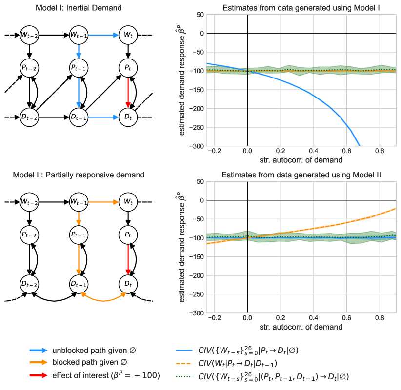
Figure 1: The effect of time dynamics on the validity of IV estimators. The left column shows the causal full time graphs of two underlying data-generating processes; the causal effect of interest is $P_{t}\to D_{t}$ (red edge). Top. In Model I, demand is inertial as $D_{t}$ structurally depends on $D_{t-1}$. The blue path is unblocked if $W_{t}$ is used as an instrument without additional controls. The naive IV estimator is, therefore, generally biased. The right column shows the corresponding estimates $\hat{\beta}^{P}$ for varying strength of structural autocorrelation in demand. Bottom. In Model II, the price-responsive part of demand is not autocorrelated; only the residual demand is. The orange path is now blocked given $\emptyset$ but unblocked given $D_{t-1}$: $D_{t-1}$ is a collider in the terminology of causal graphs. Here, the naive IV estimator is consistent. The nuisance IV estimator introduced in this paper (shown in green) is valid under both models.

To find consistent estimators for causal effects, the statistics and computer science communities have developed a framework based on structural and graphical causal models [40, 51]. In these models, each node represents a variable, and a directed edge indicates a direct causal influence. Assuming the Markov condition [33], graphical criteria such as d-separation can be employed to determine conditional independencies [8, 21]. Checking d-separation between two nodes works by assessing whether all paths between these nodes are blocked by a conditioning set and can be used to aid in the identification of valid adjustment sets or conditional instruments. For example, an IV estimator may be inconsistent if an unblocked path exists between the instrument and the dependent variable that does not go via the endogenous variable (see Section 3.1 for details). Recently, [54] have extended the graphical criteria for valid conditional IV estimators to infinite causal time series graphs [44], enabling the identification of valid conditional IV estimators in settings with time dependence.

To exploit the power of inference via causal time graphs for estimating the price elasticity of demand, we need to find an acyclic representation of a system at equilibrium. In Section 2, we do so by representing the equilibrium condition using an unobserved error term, which leads to a model with unobserved confounding. We then apply the graphical reasoning to three different demand dynamics and, based on their corresponding causal time series graphs, argue under which circumstances the naive IV estimator fails to be consistent.

In Section 3.2, we use the graph-based criteria to derive valid conditional IV estimators for each model. These estimators are based on two different ideas. First, blocking paths via conditioning: Here, the estimators achieve consistency by including lagged terms in the conditioning set; this approach leads to a class of estimators, which includes, for example, the lag-augmented local projection IV estimator [52, 37, 38] which is commonly used in macro-economics. Second, estimating nuisance effects: This approach, developed by [54], simultaneously estimates effects that are not of primary interest and whose estimates are afterward disregarded.

The proposed graphical approach allows us to systematically analyze the validity of several estimators. We further argue that observing significant differences between the estimates of presumably valid estimators can help to reject false model assumptions, thereby improving our understanding of economic dynamics. If the researcher’s assumptions encoded in the structural model are correct, two valid estimators should yield comparable results (up to finite sample errors). We argue that a statistically significant difference (i.e., non-overlapping confidence intervals) between two estimates that were considered valid ex-ante should lead the researcher to reject her model assumptions. This may be seen as an alternative approach to model validation using the reductionist approach [22].

The above findings allow us to study the problem of estimating the price elasticity of demand in the electricity market using weather-derived instruments, both on simulated data (Section 4) and on real-world data (Section 5). Estimating the price elasticity of electricity demand is important to manage the transition towards a carbon-neutral economy. Weather-dependent supply by renewables replaces flexible fossil fuel-based power plants. The price of electricity becomes highly dependent on the weather and more volatile. If demand reacts to this high-frequency price signal, less (fossil fuel-based) capacity is needed as backup facilities, and, therefore, the overall system cost decreases. Hence, getting a reliable estimate for the elasticity of demand is essential for efficient and reliable system planning. Furthermore, the application models data using high-frequency time series, increasingly available for economic studies [57]. These data differ from classical macroeconomic time series by exhibiting high autocorrelation and seasonal correlation, making it crucial to consider dynamic effects, and allowing numerous lagged terms to be included in the conditioning set without sacrificing analytical robustness.

Related literature.

There is an ongoing discussion about whether (and if so, how) causal graphs can help to solve problems in economics. Proponents argue that causal graphs representing structural causal models (SCMs) allow for the derivation of valid non-parametric estimators in a transparent and straightforward manner [51, 40, 41, 27], as exemplified by the derivation of the instrumental variable estimator by [59] for the price elasticity of demand for vegetable oil via graph-based path analysis. Opponents point out that their utility is limited to problems that can be expressed in terms of acyclic graphs and argue that this precludes a broad class of econometric problems represented by simultaneous equations such as textbook examples of supply and demand. They further argue [28, see, e.g.,] that using causal graphs does not solve problems that could not be solved using alternative frameworks such as the potential outcomes framework [39, 25, 3, 49, 4].

Despite the debate, graphs representing structural equations are not alien to econometrics, especially not to identification in time series. For example, [55] and [58] have graphically represented causal dependencies between variables in economic models over time, using what they call ‘arrow scheme’. Arguably, they have not been widely adopted, as they were inherently tied to what [58] coined the ‘causal chain model’, which posits that economic processes are recursive. In this context, recursive means that each variable of the system depends unidirectionally on the preceding variables in a sequential manner. The arrow schemes thus conflict with the prevailing notion that economic systems are generally in equilibrium and should be modeled using simultaneous equations [9, see, e.g.,], where variables are determined jointly and can influence each other simultaneously. Our approach is different as it proposes an acyclic representation of a system at equilibrium.

Causal time graphs also speak to the literature on identifying dynamic causal effects in macroeconomic time series. Macroeconomic applications focus on estimating dynamic causal effects, known as impulse response functions at different horizons $h$, that is, the response of a (macro)economic system at time $t+h$ to a shock at time $t$. A recent and popular approach for identification is to use a local projection IV estimator [31, 47, 52], which is essentially a sequential multivariate IV regression to identify the effect of price on demand at different time horizons, i.e., of $P_{t}\to D_{t}$, $P_{t}\to D_{t+1}$, $\cdots$, $P_{t}\to D_{t+h}$. The lag-augmented local projection IV estimator [46, 38] can be represented in the CIV-notation (see estimator $\#4$ in Section 3). The conditional IV criteria provide a means to decide its validity: they offer a non-parametric proof in settings where local projection IV is consistent and motivate an example in which it is not (see Section 3.2). Furthermore, the graph-based analysis provides a straightforward explanation for recent findings in this literature, such as the relevance of the lead-lag exogeneity of the instrument [52], and the robustness to model misspecification [46, 38].

Hence, formulating the problem of estimating the elasticity of demand using causal time graphs allows us to use simple, graphical criteria to determine which IV-based estimators are generally consistent and to avoid biases introduced by neglecting the time dependencies. Thus, we believe that this paper demonstrates the value of using graphs in econometrics.

2 Causal Representation of Autocorrelated Equilibrium Systems

This section links the economic equilibrium model of autocorrelated price and demand with structural causal models [51, 40, 45] and (causal) graphical models [33, 51, 40] in the context of time series data [42, e.g.,].

We propose a formalization of the equilibrium relationship that models the system of simultaneous equations as a system with time-instantaneous hidden confounding between price and demand. It serves both as an observational model and as an interventional model [43] considering interventions on the instrument (here wind) and price but not on demand. The formalization allows for a straightforward representation as a marginalized graph without cycles, a directed acyclic graph (DAG).

Section 2.1 introduces the general procedure by applying it to a model that postulates that demand is generated by an autoregressive process in which the current demand structurally depends on current prices and the immediate past of demand, i.e., demand features a direct structural autocorrelation (see Equation (1)). In Section 2.2 we introduce two alternative models with different assumptions on the intertemporal structural relations. Each model generates a time series of autocorrelated demand (see the simulations in Section 4), but they have different implications for the validity of conditional instrumental variable estimators (see Section 3). While we do not claim that these three models are an exhaustive representation of possible demand structures [22, see], each of them builds on plausible assumptions (see, for example, the discussion on electricity markets in Section 5).

2.1 Equilibrium System with Inertial Demand (Model I)

We first model demand as a structural equation, where current demand $D_{t}$ depends structurally on the price $P_{t}$, past demand $D_{t-1}$ (we refer to this dependence as direct structural autocorrelation or simply structural autocorrelation), and an i.i.d. error term $U_{t}^{D}$. Assuming linearity, the demand equation then reads

$$\textit{Model~{}I:}\qquad D_{t}\coloneqq D_{0}+\beta^{P}P_{t}+\beta^{D1}D_{t-1}+U^{D}_{t}.$$ (1)

Here, $\beta^{P}$ is the slope of the demand equation and the causal (or structural) parameter of interest.

Similarly, for all $t\in\mathbb{Z}$ we assume for supply $S_{t}$:

$$S_{t}\coloneqq S_{0}+\gamma^{P}P_{t}+\gamma^{W}W_{t}+U^{S}_{t},$$ (2)

where $W_{t}$ is exogenous, $U_{t}^{S}$ is an i.i.d. error term, and $\gamma^{P}$ is the slope of the supply equation. The structural equation of $W_{t}$ does not depend on $P_{t}$ and is independent of $U_{t}^{S}$ and $U_{t}^{D}$.

At equilibrium, demand equals supply, and the equilibrium price clears the market. This yields a structural constraint, the equilibrium condition for $P_{t}$: for all $t$ we have

$$S_{t}=D_{t}.$$ (3)

The demand and supply equations (1) and (2) are structural in $(P_{t},D_{t-1})$ and $(P_{t},W_{t})$, respectively, in that they hold under interventions on these variables. Using the notation of potential outcomes [39, 49, 29, 23] we can equivalently write them in the form $D_{t}(p)\coloneqq D_{0}+\beta^{P}p+\beta^{D1}D_{t-1}+U^{D}_{t}$ and $S_{t}(p,w)\coloneqq S_{0}+\gamma^{P}p+\gamma^{W}w+U^{S}_{t}$, where for fixed realisations of $U^{S}_{t}$ and $U^{D}_{t}$, the quantities $D_{t}(p)$ and $S_{t}(p,w)$ denote the potential outcomes of demand and supply at time $t$ for $p$ and $p$ and $w$, respectively.

From the structural equations for demand (1) and supply (2), and the equilibrium constraint (3) we get the following expression for prices at equilibrium:

$$\textit{Model~{}I:}\qquad P_{t}=\frac{S_{0}-D_{0}}{\beta^{P}-\gamma^{P}}+\frac{\gamma^{W}}{\beta^{P}-\gamma^{P}}W_{t}-\frac{\beta^{D1}}{\beta^{P}-\gamma^{P}}D_{t-1}+\frac{U^{S}_{t}-U^{D}_{t}}{\beta^{P}-\gamma^{P}},$$ (4)

where we assume that $\beta^{P}-\gamma^{P}\neq 0$, a prerequisite of market clearing.

To construct estimators for $\beta^{P}$, we exploit that the equations for demand and price, together with the equations for $W_{t}$ and $U_{t}^{D}$ form a structural causal model (SCM) [40, 5] or, more precisely, an adaption of an SCM which allows for time series models [44, 42]. (As an SCM, the system then allows for a graphical representation, with respect to which the distribution satisfies the Markov condition [40, 34].) In short, here, an SCM is a set of structural equations $X^{j}_{t}\coloneqq f^{j}(\mathrm{PA}(j,t),\epsilon^{j}_{t}))$, $j\in\{1,\ldots,d\}$, where $\mathrm{PA}(j,t)$ are the parents of $X^{j}_{t}$ and $\epsilon^{j}_{t}$, $t\in\mathbb{Z},j\in\{1,\ldots,d\}$, are jointly independent random error variables. In the example of Model I, when choosing $D_{t}$ to be $X^{1}_{t}$, we have $\mathrm{PA}(1,t)=(P_{t},D_{t-1},U^{D}_{t})$ and, when choosing $P_{t}$ to be $X^{2}_{t}$, we get $\mathrm{PA}(2,t)=(W_{t},U^{D}_{t},D_{t-1})$. We provide a formal mathematical introduction to structural causal models for time series in Appendix A.1.

The SCM models the observed distribution and intervention distributions, where we intervene on $W_{t}$ and $P_{t}$; interventions on $D_{t}$ are not modelled even though $D_{t-1}$ appears in the price Equation (4) – the reason is that we have used (1) in deriving (4). In this sense, the price equation is not structural in $D_{t}$. Thus, here, we use SCMs to construct consistent estimators and not to model all causal relationships. Using an SCM to model interventions on some but not all variables is similar in spirit to the decision-theoretic framework by [13].

Importantly, as a result of the equilibrium constraint, the variable $U_{t}^{D}$ appears in both the demand and price equations, yielding a confounder between price and demand. Since $U_{t}^{D}$ is unobserved in practice, we have thus transformed a system of equilibrium relationships into a system with a hidden confounder $U_{t}^{D}$ between $P_{t}$ and $D_{t}$.

We now represent the structure of the SCM as a directed acyclic graph (DAG) $\mathcal{G}$; each variable in the SCM corresponds to a vertex in the graph, and vertices in the graph are connected by directed edges. More precisely, we connect two nodes $u$ and $v$ by a directed edge from $u$ to $v$ if $u$ is a causal parent of $v$. When we construct a graph of a time series, we obtain a full time graph $\mathcal{G}_{FT}$. Connecting the different steps above, the structural causal model defined by the equations (1)–(4) and $W_{t}=\beta^{W}W_{t-1}+U_{t}^{W}$ induces the marginalized DAG shown in Figure 2.

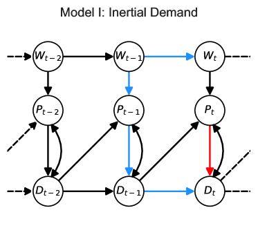
Figure 2: (Marginalized) graphical representation of Model I representing an inertial demand equation given by the structural equations (1) and (4). The causal effect of interest is highlighted in red: the effect of price on demand $P_{t}\to D_{t}$. The equilibrium constraint that supply equals demand results in bidirected edges $P_{t}\leftrightarrow D_{t}$. The blue path highlights why a naive IV estimator using $W_{t}$ as an instrument generally fails to estimate the magnitude of $P_{t}\to D_{t}$ consistently: it does not account for the confounding $W_{t}\leftarrow W_{t-1}\to P_{t-1}\to D_{t-1}\to D_{t}$ (see also Section 3).

2.2 Alternative Demand Equations

We now present two alternative models that can also generate autocorrelated time series but with different structural dependencies in time. First, Model II (heterogeneous demand) assumes that aggregate demand consists of two types: the first, $A_{t}$, is price-sensitive but not directly structurally dependent on its own past, and the second, $B_{t}$, is price-insensitive and exhibits a direct structural dependency in time. In the case of electricity markets, this distinction by price sensitivity can be motivated by the fact that a part of demand is not exposed to high-frequency price fluctuations, such as retail consumers without real-time pricing. The corresponding structural equations read

$$\begin{split}\textit{Model~{}II:}\qquad D_{t}&\coloneqq A_{t}+B_{t}=(A_{0}+\beta^{P}P_{t}+U^{A}_{t})+(B_{0}+\beta^{B1}B_{t-1}+U^{B}_{t})\\ &=D_{0}+\beta^{P}P_{t}+\beta^{B1}B_{t-1}+U_{t}^{D},\end{split}$$ (5)

where $D_{0}\coloneqq A_{0}+B_{0}$ and $U_{t}^{D}\coloneqq U_{t}^{A}+U_{t}^{B}$. The price equation becomes

$$\textit{Model~{}II:}\qquad P_{t}=\frac{S_{0}-D_{0}}{\beta^{P}-\gamma^{P}}+\frac{\gamma^{W}}{\beta^{P}-\gamma^{P}}W_{t}+\frac{\beta^{B1}}{\beta^{P}-\gamma^{P}}B_{t-1}+\frac{U^{S}_{t}-U^{D}_{t}}{\beta^{P}-\gamma^{P}}.$$ (6)

Figure 3 (left) depicts the corresponding graph.

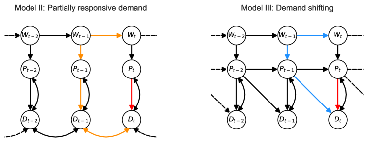
Figure 3: (Marginalized) graphical representation of alternative demand equations. Left: Model II (Partially Responsive Demand): Aggregate demand can be divided into two types as in (5), one being price-exposed and not autocorrelated, one not exposed to prices and with inertia. Richt: Model III (Demand shifting): Demand depends on the price in two time steps, current and lagged, as in (7). Thus, the model assumes that processes or systems can be shifted in time, similar to a simplified representation of a cross-price response. The blue path highlights why a naive IV estimator fails to estimate the causal effect from price on demand in the presence of cross-price elasticity (CIV1) is violated, see Section 3); by contrast, the orange path does not yield a similar violation.

Second, Model III introduces another type of time dependence. In a high-frequency time series, we expect a potential for demand optimization over time because consumption shortly before $t$ may be a substitute for consumption at time $t$. Consumers may respond to price differentials and shift their demand over time, such as deferring charging an electric vehicle. Figure 3 (right) shows a simplified cross-price elasticity in response to the realization of the price at time $t-1$. The corresponding equations are

$$\textit{Model~{}III:}\qquad D_{t}\coloneqq D_{0}+\beta^{P}P_{t}+\beta^{P1}P_{t-1}+U^{D}_{t}$$ (7)

and

$$\textit{Model~{}III:}\qquad P_{t}=\frac{S_{0}-D_{0}}{\beta^{P}-\gamma^{P}}+\frac{\gamma^{W}}{\beta^{P}-\gamma^{P}}W_{t}+\frac{\beta^{P1}}{\beta^{P}-\gamma^{P}}P_{t-1}+\frac{U^{S}_{t}-U^{D}_{t}}{\beta^{P}-\gamma^{P}}.$$ (8)

3 Graph-based IV Estimation in Equilibrium Models

Next, we discuss sufficient conditions for valid instrumental variable (IV) estimation in equilibrium systems with a time series structure (Section 3.1). To do so, we exploit graphical conditions for validity of conditional IV (CIV) estimators [8, 21], which have recently been extended to time series settings [54]. In Section 3.2 we apply these CIV principles to the three models introduced in Section 2 and present several valid CIV estimators. We argue that discrepancies between them can inform researchers about the validity of the underlying models and assumptions.

3.1 Conditional IV Estimation in Time Series

For constructing valid estimators we make use of the concept of d-separation (short for directed separation) [40]. D-separation is a purely graphical criterion connected to conditional independences of random variables via the Markov condition [33]. [40]’s original formulation considers finite graphs; here, we use a version that is adapted to (marginalized) infinite time series graphs.

Definition 3.1 (Pearl’s d-separation [40]).

Let $\mathcal{G}$ be the marginalized version of an acyclic directed full time graph [44], which contains a node for each variable and time point, with vertices $V=\mathbb{Z}\times\{1,\dots,d\}$, and let $i_{1},\dots,i_{m}$ be a path between vertices $i_{1}$ and $i_{m}$ in $\mathcal{G}$. We say that the path $i_{1},\dots,i_{m}$ is blocked by the set of variables $S\subseteq V\setminus\{i_{1},i_{m}\}$ if there exists $k\in\{2,\dots,m-1\}$ such that either

1. $i_{k}\in S$ and $i_{k}$ is not a collider on the path $i_{1},\dots,i_{m}$, or

2. $i_{k}$ is a collider on the path and $(\{i_{k}\}\cup\mathrm{DE}(i_{k}))\cap S=\emptyset$, where $\mathrm{DE}(i_{k})$ are the descendants of $i_{k}$;

if a path is not blocked by $S$, we say it is unblocked, given $S$. For three mutually disjoint sets of vertices $A,B,S\subset V$, we say that $A$ and $B$ are d-separated by $S$ if all paths between $A$ and $B$ are blocked by $S$. If this is the case, we write

$$A\perp\!\!\!\perp_{\mathcal{G}}B\mid S.$$

The concept of d-separation helps us to construct valid IV estimators in time series. The following statement is an adapted version of Theorems 5 and 8 of [54]. Let $d,d^{\prime}\in\mathbb{N}$, $d\leq d^{\prime}$ and let $V^{\prime}=\mathbb{Z}\times\{1,\dots,d^{\prime}\}$. Consider a linear SCM for time series over variables $X_{V^{\prime}}$ and let $\mathcal{G}$ be the induced marginalized version of an acyclic directed full time graph with vertices $V=\mathbb{Z}\times\{1,\dots,d\}$. Let $\mathcal{I},\mathcal{X},\mathcal{B},\{Y\}\subseteq V$ have zero means and finite second moments and let $\beta\in\mathbb{R}^{|\mathcal{X}|}$ be the causal coefficient with which $X_{\mathcal{X}}$ enters the structural equation for $X_{Y}$, that is,

$$X_{Y}=\beta^{T}X_{\mathcal{X}}+\gamma^{T}X_{K}+\epsilon^{Y},$$ (9)

for some variables $X_{K}\subseteq X_{V}\setminus X_{\mathcal{X}}$ (some of the components of $\beta$ can be zero, so not all variables in $X_{\mathcal{X}}$ have to be parents of $X_{Y}$).

One then considers the following three requirements on $\mathcal{I},\mathcal{X},{\mathcal{B}}$ and $Y$, the CIV criteria:

• $\mathcal{I}$ and $Y$ are d-separated given $\mathcal{B}$ in the graph $\mathcal{G}_{\mathcal{X}\not\rightarrow Y}$, which denotes the graph obtained when removing all direct edges from $\mathcal{X}$ to $Y$ from $\mathcal{G}$.

• $\mathcal{B}$ is not a descendant of $\mathcal{X}\cup\{Y\}$ in $\mathcal{G}$.

• the matrix $\mathbb{E}[\text{cov}(X_{\mathcal{X}},X_{\mathcal{I}}|X_{\mathcal{B}})]$ has rank $|\mathcal{X}|$, that is, full row rank.

(CIV1) and (CIV2) are properties of the underlying causal graph, (CIV3) is a property of the induced distribution.

Assume we have observations at time points $1,\ldots,T$. If an estimator is based on $\mathcal{I},\mathcal{X},{\mathcal{B}}$ such that requirements (CIV1), (CIV2) and (CIV3) are met, we call it a valid CIV estimator. In this case,

$$\hat{\beta}\coloneqq\arg\min_{b}\|\hat{\text{cov}}(X_{Y}-b^{T}X_{\mathcal{X}},X_{\mathcal{I}}|X_{\mathcal{B}})\|,$$ (10)

is a consistent estimator for $\beta$ if $T\to\infty$ (for a detailed definition of $\hat{\beta}$ and its closed form solution see Appendix B). We call $\hat{\beta}$ the conditional instrumental variable (CIV) estimator and denote it by $\mathrm{CIV}(\mathcal{I}\mid\mathcal{X}\to Y\mid\mathcal{B})$.

If at least one of the conditions is not met, then we call the estimator invalid and, in general, it may not be consistent [21] (but exceptions exist). In the special case, however, that (CIV1) and (CIV2) are satisfied but (CIV3) is not (this is related to weak instrument settings), any estimation technique that comes with valid inference yields unbounded confidence sets containing the true causal effect with large probability. In this sense, it is therefore not necessary to test for the validity of (CIV3).

3.2 Consistent Estimation of Price Elasticities

We now apply the CIV criteria to derive valid estimators for the Models I–III presented in Section 2. For example, consider Model I from Section 2.1. The model is described by Equations (1) and (4), and the corresponding marginalized time graph in Figure 2. The naive IV estimator $\#1$ that neglects time dependencies can be written as $\mathrm{CIV}(W_{t}\mid P_{t}\to D_{t}\mid\emptyset)$, that is, we set $X_{\mathcal{X}}=(P_{t})$, $X_{Y}=\{D_{t}\}$, $X_{\mathcal{B}}=\emptyset$ and $X_{\mathcal{I}}=(W_{t})$. We see that (CIV1) is not satisfied: After removing the edge $P_{t}\to D_{t}$ in Figure 2, we obtain the graph $\mathcal{G}_{P_{t}\not\rightarrow D_{t}}$. In this graph, there are several unblocked paths given $\emptyset$ through $W_{t-1}$ that connect the instrument $W_{t}$ to the dependent variable $D_{t}$. An example is the blue path in Figure 2, $W_{t}\leftarrow W_{t-1}\to P_{t}\to D_{t-1}\to D_{t}$, given $X_{\mathcal{B}}=\emptyset$. $W_{t}$ is therefore not d-separated from $D_{t}$.

We provide an overview of some available estimators and their validity in Table 1. We group CIV estimators along two main concepts. The first approach uses a selection of path-blocking variables as the conditioning set. Such a conditioning set can contain past realizations of the instrument $W_{t}$, the endogenous variable $P_{t}$, or the outcome variable $D_{t}$. For example, the estimator $\#3$ $\mathrm{CIV}(W_{t}\mid P_{t}\to D_{t}\mid D_{t-1})$ contains only one lag of the outcome variable; it is valid for Model I. The estimator $\#2$, $\mathrm{CIV}(W_{t}\mid P_{t}\to D_{t}\mid\{W_{t-s}\}_{s=1}^{L})$, contains $L$ lags of the instrument and is valid for Models I–III. Intuitively, by including the past realizations of the instrument in the conditioning set, we block the path starting with $W_{t}\leftarrow W_{t-k}$ for some $k\geq 1$. The estimator $\#2$ is valid under a strictly more general model class: for example, it is even valid for any model yielding a (marginalized) graph, in which $P_{t}\rightarrow D_{t}$ is the only directed path between $P_{t}$ and $D_{t}$, and the set of parents of $W_{t}$ is a subset of $\{W_{t-1},\ldots,W_{t-L}\}$. This model class contains Models I, II, and III. We therefore consider $\#2$ our benchmark estimator. The second approach relies on the concept of simultaneously estimating nuisance effects. Estimator $\#8$, $\mathrm{CIV}(\{W_{t-s}\}_{s=0}^{L}\mid(P_{t},P_{t-1},D_{t-1})\to D_{t}\mid\emptyset)$, for example, adds two additional nuisance covariates to $\mathcal{X}$. It estimates a three-dimensional effect and later ignores two of its components.

	Estimator	Model I Figure 2	Model II Figure 3 (left)	Model III Figure 3 (right)
	Naive IV
$\#1$	$\mathrm{CIV}(W_{t}\mid P_{t}\to D_{t}\mid\emptyset)$	✗	✓	✗
	Conditional IV
$\#2$	$\mathrm{CIV}(W_{t}\mid P_{t}\to D_{t}\mid\{W_{t-s}\}_{s=1}^{L})$	✓	✓	✓
$\#3$	$\mathrm{CIV}(W_{t}\mid P_{t}\to D_{t}\mid D_{t-1})$	✓	✗	✗
$\#4$	$\mathrm{CIV}(W_{t}\mid P_{t}\to D_{t}\mid\{W_{t-s},P_{t-s},D_{t-s}\}_{s=1}^{L}$)	✓	✓	✓
	Nuisance IV
$\#5$	$\mathrm{CIV}(\{W_{t-s}\}_{s=0}^{L}\mid(P_{t},D_{t-1})\to D_{t}\mid\emptyset)$	✓	✓	✗
$\#6$	$\mathrm{CIV}(\{W_{t-s}\}_{s=0}^{L}\mid(P_{t},P_{t-1})\to D_{t}\mid\emptyset)$	✗	✓	✓
$\#7$	$\mathrm{CIV}(\{W_{t-s}\}_{s=0}^{L}\mid(P_{t},P_{t-1})\to D_{t}\mid D_{t-1})$	✓	✗	✓
$\#8$	$\mathrm{CIV}(\{W_{t-s}\}_{s=0}^{L}\mid(P_{t},P_{t-1},D_{t-1})\to D_{t}\mid\emptyset)$	✓	✓	✓

Table 1: Estimators and their validity for the causal effect $\beta^{P}$ from $P_{t}\to D_{t}$ for Models I–III

Special cases for a valid naive IV estimator.

Even though the naive IV estimator does not necessarily satisfy (CIV1), there are special cases in which the naive estimator is valid, as visualized in Figure 4. These occur i) when the instrumental time series is i.i.d., or ii) when demand is not directly affected by its past realizations, or iii) when there is no response to prices, i.e., $\beta=0$. In all three cases, no unblocked path exists (given $\emptyset$) from $W_{t}$ to $D_{t}$ through the past.

Figure 4: Graphical representation of special cases of Model I, for which naive IV is a valid estimator. Left: The instrument is i.i.d.  i.e., not autocorrelated. Middle: The demand function is not autocorrelated. Right: The demand is not responsive to prices.

Local Projection IV Estimator.

Estimator $\#4$ in Table 1 is the lag-augmented local projection IV estimator from the macroeconomic literature on identifying impulse response functions [52, 37]. In CIV notation, the local projection IV estimator for the time horizon $h=0$, i.e., the effect of $P_{t}\to D_{t}$, can be written as $\mathrm{CIV}(W_{t}\mid P_{t}\to D_{t}\mid\{W_{t-s},P_{t-s},D_{t-s}\}_{s=1}^{L})$; thus, the local projection IV estimator is a special case of a CIV estimator with lags of the instrumental, endogenous, and dependent variable in the conditioning set, since it also relies on the concept of blocking path to achieve validity. To achieve validity, however, including the lags of the instrument would be sufficient (see estimator $\#2$). If, however, in Model I, there is additional hidden confounding between $W_{t}$ and $P_{t-1}$, and $D_{t}$ and $P_{t-1}$, $\#4$ is invalid, while $\#2$ would still be valid. Estimator $\#2$ is valid across a larger model class.

Model validation.

The existence of several valid IV estimators allows us to learn about the structure of the demand response. We can assume a particular structure of the demand equation, but we do not know ex-ante whether this assumption holds. The ability to derive multiple supposedly valid estimators for a structural model can be used to test this assumption. For example, if Model II describes the true time dependencies, the confidence intervals of all estimators but number $\#3$ in Table 1 should overlap with high probability. This can be tested from observational data. If the confidence intervals do not overlap, one should reject Model II.

4 Simulating electricity market data

We now evaluate the CIV estimators of Section 3.2 in a controlled environment motivated by the German electricity market (see Section 5). We empirically quantify the bias that arises when using invalid estimators and compare the empirical performances of the CIV estimators (including nuisance IV estimators). We also show that the autocorrelation of the response time series does not suffice to correct for the bias of invalid estimators.

Data generation.

We generate multiple datasets containing three hourly time series: a supply-shifting instrumental time series, wind generation, the equilibrium electricity demand, and the equilibrium electricity price. We model wind generation as an AR$(L)$ process with autocorrelation coefficients derived from observed wind generation data in Germany in 2019 (see Appendix D.1 for data sources). The supply equation corresponds to Equation (2) with $\gamma^{P}=+500$ MW/(EUR/MWh). It is parameterized so that every unit of generated wind electricity is immediately offered to the market $(\gamma^{W}=1)$. The constant $S_{0}=25,000$ MWh/h implies that there is supply even if prices drop below zero, a typical characteristic of real-world electricity markets. The errors $U_{t}^{S}$ are i.i.d. $\mathcal{N}(0,1)$. Finally, we equate the supply and the model-specific demand equation (Equation (1), (5) or (7)) to obtain hourly equilibrium prices and quantities. Unless otherwise specified, the demand equation is parameterized as follows: the own price elasticity is $\beta^{P}=-100$ MW/(EUR/MWh), the error terms of the demand equation are i.i.d. $\mathcal{N}(0,2000)$, and the constant of the demand series $D_{0}$ is chosen so that the resulting demand is stationary around the mean value of German electricity load (approximately $60$ GWh/h).

CIV estimation.

All CIV estimators are calculated with the Python package linearmodels [50], using the kernel correction for heteroscedasticity and autocorrelation robust errors (HAC).

Validity of estimators.

We validate the theoretical findings of Section 3. In Figure 5, we apply the CIV estimators specified in Table 1 to the data simulated from Model I. We find that the confidence sets of all valid estimators overlap (compare the overlap of the confidence intervals with the check marks for Model III on the right of Figure 5). Conversely, if one had assumed Model II, one would be forced to reject the associated structural assumptions since estimators $\#1$ and $\#6$ deviate from other valid estimators (e.g., $\#2$ and $\#8)$. The simulation thus underscores our argument that comparing the overlap of several presumably valid estimators provides a means of rejecting incorrect structural assumptions.

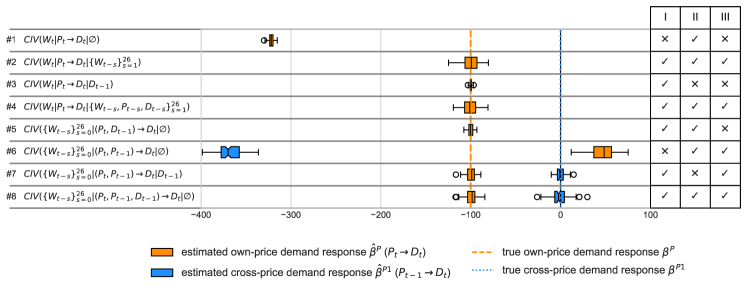
Figure 5: CIV estimates $\hat{\beta}^{P}$ of the true demand response $\beta^{P}=-100$ MW/(EUR/MWh) when data is simulated based on Model I (Figure 2). The structural autocorrelation of demand is $\beta^{D1}=0.7$. The columns on the right indicate the validity according to the CIV criteria (see Table 1).

Magnitude of bias.

We quantify the bias caused by ignoring any direct structural autocorrelation. In linear SCMs, the bias (explicitly computed by [54]) depends on the path coefficients along unblocked paths (which may be unblocked due to wrongfully including descendants of colliders in the conditioning set). Figure 6 shows the empirical percentage error of the naive IV estimator $\#1$ applied to estimate the demand response for data generated from Model I. We vary the direct structural autocorrelations of the instrumental time series $(\beta^{W})$ and the demand series $(\beta^{D1})$. For low levels of instrument autocorrelation $(\beta^{W}<0.2)$, ignoring time dependencies leads to a moderate bias $(<20\%)$. However, the resulting bias is substantial for high-frequency time series. For example, in real-world data (see Section 5), the autocorrelation of wind generation (at lag 1) can have values above 0.9. Hence, even for small levels of direct structural autocorrelation of demand, this could lead to a bias of more than $25\%$. We observe the same pattern for other combinations of models and invalid estimators (see Figure 12).

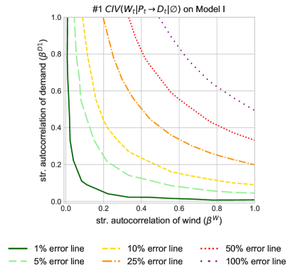
Figure 6: Isolines showing the average absolute percentage error of the point estimate as a function of the structural autocorrelation of wind (instrument) and the structural autocorrelation of demand (dependent variable). For the simulations, we divide both axes into ten equidistantly spaced autocorrelation coefficients between 0 and 1 each, based on which we run $20$ simulations with five years of data $(T=43,800)$.

Structural vs. observed autocorrelation.

Knowing the observed autocorrelation of the demand is not sufficient for correcting for the bias of the naive IV estimator $\#1$. In Figure 7, we plot the percentage error of estimator $\#1$ against the observed autocorrelation of demand (which we denote by $\alpha^{D1}$ to distinguish it from the structural autocorrelation denoted by $\beta^{D1})$. The intensity of the color indicates the value of the respective structural coefficients. The figure shows that the same level of observed autocorrelation (at lag one) can result from different structural dependencies, yielding different estimation errors. Low levels of observed autocorrelation can result in a substantial bias of $100\%$ (e.g., Model III at $\alpha^{D1}\approx 0.2)$, and observed autocorrelation up to $\alpha^{D1}\approx 0.9$ can be associated with no bias at all if the data is generated by a different model (e.g., Model II). Consequently, knowing the observed autocorrelation of demand (at lag one) is insufficient for deriving a structural model or predicting a bias.

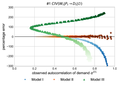
Figure 7: The percentage error of the naive IV estimator $\#1$ is shown as a function of the observed autocorrelation of demand $(\alpha^{D1})$. In each simulation we vary the structural dependencies: In Models I and II, the strengths of the structural autocorrelations, $\beta^{D1}$ and $\beta^{B1}$, are both varied between $-0.25$ and $0.99$. In each simulation we vary the structural dependencies: In Models I and II, the strengths of the structural autocorrelations, $\beta^{D1}$ and $\beta^{B1}$, are both varied between $-0.25$ and $0.99$. In Model III, $\beta^{P1}$ is varied between $-250$ MW/(EUR/MWh) and $+250$ MW/(EUR/MWh). The color intensity increases in tandem with the aforementioned ranges. For each model, we conduct $400$ simulations with a sample period of five years $(T=43,800)$.

Empirical performance of different CIV estimators.

We analyze the empirical performance of the three CIV estimators that are valid across a wide class of models: the nuisance IV estimator $\#8$, the CIV estimator $\#2$, and the CIV estimator $\#4$, which corresponds to a lag-augmented local projection IV estimator. We do so based on three indicators: Coverage, which indicates how often the $95\%$-confidence interval of $\hat{\beta}^{P}$ contains the true value $\beta^{P}$; average absolute percentage error, which averages $100\cdot|\hat{\beta}^{P}-\beta^{P}|/|\beta^{P}|$ over different simulations; and the length of the confidence interval.

Figure 8 plots the indicators as a function of the sample size for data generated from Model I. All estimators have coverage (left), confirming these approaches’ validity. However, the nuisance IV estimator $\#8$ has a smaller average absolute percentage error (middle) and yields shorter confidence intervals at smaller sample sizes (right) than both the conditional IV estimators of the most general class, $\#2$, and the lag-augmented local projection IV estimator, $\#4$. The benefit of having a large sample size becomes marginal beyond five years but holds regardless of the structural model (see Figure 14 and Figure 15). Thus, while the estimators that rely on blocking the blue path in Figure 2 by conditioning, $\#2$ and $\#4$, are conceptually simple and retain validity across a large class of models, the estimator that relies on estimating nuisance effects, $\#8$, in the above setting outperforms them, thereby providing a useful alternative for smaller sample sizes.

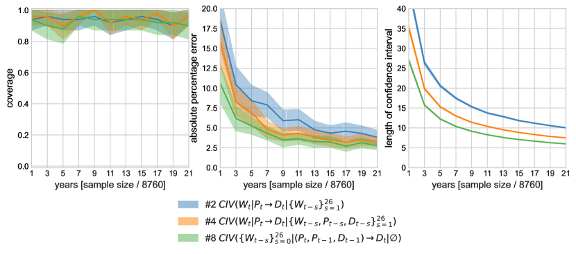
Figure 8: Evaluation of the statistical performance of conditional vs. nuisance IV estimators for Model I based on the performance indicators: (left) coverage, (middle) the average absolute percentage error, and (right) the length of the confidence interval. $(\beta^{D1}=0.9$.) The shaded areas represent the 95% confidence intervals. For each year, we run $50$ simulations.

5 Estimation of the Price Elasticity of Hourly German Electricity Demand

We estimate the own-price elasticity of the aggregate German electricity demand using the CIV estimators derived in Section 3. Furthermore, we discuss what the divergence between the estimators can reveal about the structure of the dynamic response.

Price elasticity of electricity demand.

Historically, electricity demand was considered inelastic, and power plants adjusted their supply according to whatever demand occurred [7, 11]. Liberalization, digitalization, and decarbonization over the last three decades have started to change that. After liberalization, it soon became clear that a low elasticity of demand inflates the ability of producers to abuse market power, and policymakers took measures to promote more flexible customer behavior, e.g., by increasing the exposure of consumers to real-time pricing [7, 17]. In addition, as the role of wind and solar expands globally, price volatility increases, and the benefits of flexible demand become larger [10, 35, 26]. Policy scenario and system planning studies assume future demand to be increasingly price-elastic [1, e.g.,]. Therefore, an accurate estimate of the price elasticity of electricity demand is important for reliable system planning and appropriate policy decisions.

The electricity market.

The electricity system must always be in balance for physical reasons. The primary mechanism to equalize demand and supply is the day-ahead auction of the wholesale market. This is where generators, retail suppliers, and large industrial consumers submit their price-volume bids for each hour of the following day. Because electricity storage is expensive and limited in capacity, wholesale electricity prices are much more volatile than other commodities [10, 35, 26].

Data.

We estimate the own-price elasticity on electricity market data between October 23, 2017, and December 31, 2020 (see Table 2 for summary statistics). Electricity demand in megawatt-hours per hour (MWh/h) is defined as consumption in the joint German-Luxembourg market. The electricity price in Euro per megawatt-hour (EUR/MWh) corresponds to the clearing price of the day-ahead auction on EPEX Spot, the largest marketplace for the market zone. Wind generation is in gigawatt-hours per hour (GWh/h). A detailed description of the data and sources can be found in Appendix D.1. Whenever we exclude hours and/or split the data set, we determine the relevant lags and then perform the split.

	Mean	Std. Dev.	Min	Median	Max	Skew-ness	Kurto-sis
Consumption [GWh]	59.9	11.3	34.0	59.5	91.7	0.16	-0.7
Price [€/MWh]	38.0	17.6	-90.0	38.0	200.0	-0.35	3.8
Wind Generation [GWh]	14.1	10.1	0.1	11.6	46.1	0.87	-0.1

Table 2: Summary Statistics; $T=27,072$ after removing holidays.

Identification.

To overcome the endogeneity problem induced by the equilibrium condition, we use wind power generation as an exogenous time series. Wind speed and wind power generation are commonly used as supply shifting instruments because they are relevant and credibly exogenous [6, 32, 17, 24]. The assumption that the structural equation of wind power generation does not depend on the price of electricity is based on the argument that renewable generators have marginal costs close to zero. Additionally, most German wind power generators also receive a subsidy per unit of electricity produced, which induces an opportunity cost of not producing, even if prices are negative.

We follow [24] in proposing that wind power is independent of the noise terms of demand and supply after conditioning on suitable covariates. While it is reasonable to assume that wind power does not affect demand in any way other than through the price of electricity, we expect the existence of common causes such as seasonality and weather events. We therefore condition on the following covariates: seasonal dummies (hour of the day, day of the week, and month of the year) and weather controls (sunlight, and heating and cooling degrees). Furthermore, we include other covariates to increase the precision of the estimate, namely commodity prices (natural gas, coal, and emission allowances), solar PV generation, and other calendar controls (school vacations by state and a variable for the last week of the year).

In Models I–III, we assume $W_{t}$ to have a structural autocorrelation of on lag, and in that case, for many of the estimators, including a single time lag suffices. However, observed wind power exhibits a higher degree of autocorrelation (see Figure 18), which needs to be reflected in the construction of the different estimators (the argument remains the same). Given the observed autocorrelation pattern, we include up to $50$ lags of wind power generation in the conditioning set of the CIV estimator $\#2$ and $\#4$, and as instruments for the nuisance IV estimators $\#4$ to $\#8$. We also observe a significant autocorrelation pattern in the demand time series (this is expected if there is indeed a causal effect from wind power generation on demand, but it may have other sources, too).

Models of electricity demand.

Electricity demand features two main mechanisms that can imply structural correlations in time (for a comprehensive classification of demand response in the electricity market, see [2]). First, some electricity-consuming processes run for extended periods and cannot be switched on and off by the hour. This includes many industrial activities spanning an entire work shift and residential activities such as washing machines with multi-hour programs. Therefore, it is likely that the demand at time $t$ depends on the load of the previous hours, as in our Model I. Second, some electricity-consuming processes can be shifted in time to exploit power price differentials. Such ‘load shifting’ may be done by scheduling industrial processes during low-price hours and by postponing charging electric vehicles, for example. Model III represents a simplified version of the shifting dynamic, where demand $D_{t}$ also depends on the lagged price $P_{t-1}$.

Our alternative demand Model II assumes that processes or systems can be divided into two types: one that is price-exposed and reacts instantaneously and one that is inertial and not exposed to price variations. This model is motivated by the observation that most retail consumers are not exposed to real-time prices and that only the remaining consumers can respond to prices. For simplicity, we assume that these remaining consumers can regulate their processes individually for each hour.

Additional assumptions about the demand equation.

The models we consider make additional assumptions about the demand response. First, they posit that the functional form of the resulting demand equation depends linearly on price. To show that dynamics matter irrespective of the functional form, we include results for the assumption of an exponential relationship in Figure 9. Second, the models assume that the elasticity is constant across hours and seasons. This implies that consumers who are active during the day have, on average, the same elasticity as consumers who are active at night. We investigate the relevance of this assumption in more detail in a robustness analysis in Appendix D.2.

Quantitative results.

Figure 9 gives the quantitative results. The CIV estimators $\#2$ and $\#4$, and the nuisance IV estimator $\#8$, which are valid across a large model class, have overlapping confidence intervals. All three estimate a linear demand response $\hat{\beta}^{D}$ of approximately $-200$ MW/(EUR/MWh). The log-log specification yields a unitless estimate of $-0.1$. An intervention on supply by a quantity similar to the magnitude of one standard deviation of the instrument, $693$ MW, leads to a predicted price change of EUR $-0.64$, and thus an increases in the equilibrium quantities of $140$ MW.

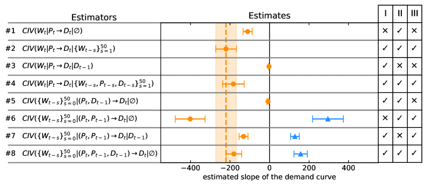
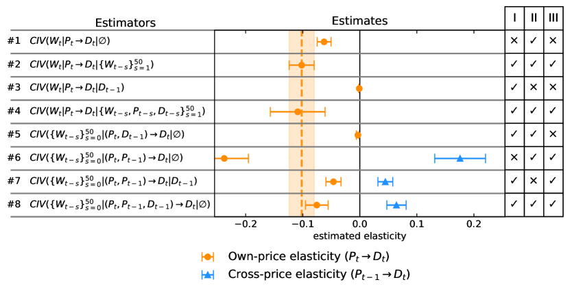
Figure 9: The own-price elasticity of aggregated German electricity demand, obtained by CIV estimators (top: linear specification; bottom: log-log specification). The highlighted area corresponds to the confidence interval of estimator $\#2$. The tables on the right are reproductions of Table 1, showing the validity of each strategy for the structural causal models described in Section 2.

Overlap pattern.

We can also analyze the pattern of the different CIV estimators to learn about the real-world dynamics of electricity demand response. First, we can reject a linear model without relevant structural autocorrelation. Figure 9 shows that the pattern of estimators does not correspond to the pattern that we would expect if real-world dynamics would not bias a naive estimate: The confidence intervals of the benchmark estimator and the naive IV estimator do not overlap, for example. Also, we can reject that the observed autocorrelation in the time series is only caused by an autocorrelation in the residual demand, as in Model II: the estimators $\#1$ and $\#5$ yield smaller absolute values than estimators $\#2$ and $\#8$ for the own-price elasticity, with non-overlapping confidence sets. Second, our results indicate that the dynamics of electricity markets are more complex than suggested by the simple Models I, II, and III because, taken in isolation, none of the models is sufficient to explain the disagreement between the estimators. Our approach only allows us to falsify structural assumptions but not to confirm them.

Robustness.

As mentioned at the beginning of this section, we make the strong assumption that the demand elasticity is constant across hours. However, different consumers are active in the electricity market at other times of the day, resulting in a changing composition of consumer elasticities. To account for this temporal heterogeneity, [32] investigate the level of demand response by the hour of the day, and [24] additionally analyze heterogeneity by weekday and season. In Appendix D.2, we provide a robustness analysis that divides the hours into on-peak and off-peak periods (with lags of the variables extending into the respective other phase as needed). The results show that the overlap pattern holds primarily for on-peak demand. This period is also when we would expect the highest demand response, and the quantitative results of the benchmark estimator $\#2$ are correspondingly higher. In contrast, the structural dynamics during off-peak periods (i.e., at night) suggest a different dynamic, which could be investigated further with our proposed method.

Intervention.

Causal inference is concerned with predicting the effect of interventions on a system. $\hat{\beta}^{D}$ is an estimate of the structural coefficient $\beta^{D}$ of the demand equation. It can be interpreted as the demand response to a hypothetical intervention on the equilibrium price. If $\beta^{D}$ were indeed $-200$ MW/(EUR/MWh) and it were possible to reduce the price by EUR $1$, demand would increase by $200$ MWh/h (see Figure 10 (middle)). We call this intervention hypothetical because a direct and isolated intervention on the price only would yield a market that is out of balance: If one were to set the price to $p_{\mathrm{fix}}$, not only would the quantity demanded change, but so would the quantity supplied, resulting in an imbalanced market $(S(p_{\mathrm{fix}})\neq D(p_{\mathrm{fix}}))$. One may also consider demand or supply shocks that shift or alter the demand or supply curve. For example, a supply shock that occurs regularly is changing weather conditions that affect the availability of renewable energy. Figure 10 (right) illustrates a supply shock that leads to the equilibrium quantities $Q$. Unlike the example of a hypothetical intervention on the price, in this scenario, equilibrium quantity and price are endogenous, ensuring that the market clears.

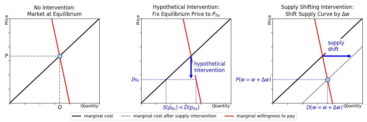
Figure 10: Illustrations of conceptually different interventions in a market at equilibrium. Left: Market at equilibrium, i.e., the state without any intervention. Middle: Hypothetical intervention on the equilibrium price, fixing the equilibrium price at $P_{\mathrm{fix}}$. The demand elasticity is sufficient to calculate the effect of the intervention on the quantity demanded. However, the market does not clear because marginal cost is less than marginal willingness to pay. Richt: Factual intervention $X_{shift}$ that shifts the supply curve outward, leading to a new market equilibrium.

6 Conclusion

This paper demonstrates the advantages of using directed acyclic graphs to estimate the price elasticity of demand with autocorrelated instruments. While it is well known that autocorrelation can lead to biased estimates, relying solely on observed autocorrelation and statistical tests can mislead researchers seeking valid estimators. Causal graphs allow us to express structural assumptions transparently, understand biasing dynamics, derive multiple valid estimators, and ultimately test the validity of assumptions about structural dependencies over time. Suppose economists wish to benefit from causal time graphs. In that case, they can do so without abandoning the idea of simultaneous determination of supply and demand: equilibrium relationships can be represented in DAGs similarly to a time-instantaneous hidden confounding.

The graphical CIV criteria provide two different approaches to valid IV estimators. One approach blocks paths by including lagged terms in the conditioning set, and the other simultaneously estimates nuisance effects. While the former is more robust to model misspecification, the latter can be more powerful at small sample sizes.

We have applied the above to estimate the own-price elasticity of electricity demand under three competing structural assumptions: a model in which demand exhibits inertia, a model in which demand additionally depends on previous prices and a model of heterogeneous response. We have shown through simulations that each model can manifest identical levels of observed demand autocorrelation, illustrating that the observed correlation alone cannot predict potential bias. The estimates diverge when conditional IV estimators are applied to German electricity demand. This suggests that the widely used IV estimator, which ignores time dynamics, cannot identify the own-price elasticity without significant bias.

Looking ahead, the similarity between the CIV estimators derived from causal graphs and the lag-augmented local projection IV estimator calls for an extension of causal time graphs to estimate impulse response functions. Causal full time graphs can help strengthen the intuition behind recent results in this literature. To give just three examples: First, local projection IV estimators are found to identify the same impulse response function as a vector autoregressive model with the instrument ordered first [46] . Second, local projection IV is found to be robust to misspecification [38], which could be related to the lag-augmented local projection IV estimator blocking the same unblocked path multiple times. Third, [37] prove that for a local projection IV estimator, the use of Eicker-Huber-White heteroskedasticity-robust standard errors is sufficient without further needing to correct for autocorrelation. This result could be because the lagged terms in the conditioning set already sufficiently account for structural and, hence, bias-inducing autocorrelation. Going beyond recent findings, the graphical approach would further provide nonparametric proof, and the CIV criteria allow for a transparent analysis of the validity of the local projection IV estimator under hidden confounding.

Thus, as this paper has shown, the graphical approach is a powerful addition to the toolkit of every economist working with data structured as a time series, with many applications yet to be explored.

7 Funding

Researchers from the Hertie School gratefully acknowledge financial support from the German Federal Ministry of Education and Research through the ARIADNE Project (FKZ 03SFK5K0). Lion Hirth is owner and director of Neon Neue Energieökonomik GmbH, an energy economics consulting firm. Oliver Ruhnau is owner and director of tournesol energy GmbH, an energy consulting and software firm.

Appendix A Causal Models for Time Series

This appendix provides a formal introduction to causal inference for time series. First, we give a formal definition of structural causal models (SCM), followed by an introduction to directed acyclic graphs (DAGs) for time series. Finally, we introduce the concept of marginalization, which is a way to simplify the representation of graphs.

A.1 Structural Causal Models for Time Series

Let $\{U_{t}^{j}\}_{t\in\mathbb{Z},j\in\{1,\dots,d\}}$ be a set of $d$ jointly independent random error variables. The index $t$ encodes time, and the index $j$ is the time series component.

For all $j\in\{1,\dots,d\}$ let $\mathrm{PA}(j)\subseteq\{(k,s)\ |\ k\in\{0,\dots,q\},s\in\{1,\dots,d\}\}$ and $p_{j}\coloneqq|\mathrm{PA}(j)|$ be the number of elements in $\mathrm{PA}(j)$, and let $f^{j}:\mathbb{R}^{p_{j}}\times\mathbb{R}\to\mathbb{R}$ be a measurable function. The sets $\mathrm{PA}(j)$ encode the (causal) parents of $X_{t}^{j}$, which we assume do not depend on $t$. For all $j\in\{1,\dots,d\}$ and all $t\in\mathbb{Z}$ we consider the structural equations

$$X_{t}^{j}\coloneqq f^{j}\left(\mathrm{PA}(j,t),U_{t}^{j}\right),$$ (11)

where the parents of $X^{j}_{t}$ are defined by $\mathrm{PA}(j,t)\coloneqq(X^{s_{1}}_{t-k_{1}},\dots,X^{s_{p_{j}}}_{t-k_{p_{j}}})$ with $\{(k_{1},s_{1}),\ldots,(k_{p_{j}},s_{p_{j}})\}=\mathrm{PA}(j)$, where the $(k_{i},s_{i})$ are in lexicographic order.

We further assume that there is a unique solution to (11) that is weakly stationary and that the process realization is covariance ergodic. We further assume that the induced distribution is Markov with respect to the induced graph (see Section A.2). For linear functions $f^{1},\dots,f^{d}$, which we consider in this paper, these properties are well-studied [54, see, for example,].

A.2 Directed Acyclic Graphs for Time Series

We now introduce some standard graph terminology [33, 19, 40, e.g.,], adapted to the case of infinitely many nodes. Let $V\subseteq\mathbb{Z}\times\{1,\dots,d\}$. A directed graph $\mathcal{G}=(V,E)$ is composed of nodes $V$ (also called vertices) and edges $E\subseteq V\times V$ with the restriction that for all $u,v\in V$ either $(u,v)\not\in E$ or $(v,u)\not\in E$ or both. We sometimes use the notation $v\to u$, meaning that $(v,u)\in E$.

A path in $\mathcal{G}$ is a sequence of distinct vertices $v_{1},\ldots,v_{m}$, such that an edge connects each consecutive pair of vertices. If $v_{k}\to v_{k+1}$ for all $k\in\{1,\dots,m-1\}$, we say that the path is directed from $v_{1}$ to $v_{m}$. A directed path $v_{1}\to...\to v_{m}$ such that $(v_{m},v_{1})\in E$ is called a cycle. A directed graph $\mathcal{G}$ is classified as a directed acyclic graph (DAG) if it has no cycles.

Because we deal with time series, the structural equations induce a graph with infinitely many nodes, i.e., a full time graph [44] $\mathcal{G}_{\mathrm{FT}}$ over nodes $V=\{(t,s)\ |\ t\in\mathbb{Z},s\in\{1,\dots,d\}\}$, where we draw an edge from $(t_{1},s_{1})$ to $(t_{2},s_{2})$ if $(t_{1},s_{1})\in\mathrm{PA}(t_{2},s_{2})$. We assume that the parent sets are such that $\mathcal{G}_{\mathrm{FT}}$ is directed and acyclic. We say $v\in V$ is a descendant of $u\in V$ if $v\neq u$, and there exists a directed path from $u$ to $v$. We denote the set of descendants of $u$ by $\mathrm{DE}(u)\coloneqq\{v\in V\ |\ \text{$v$ is a descendant of $u$}\}$.

A.3 Graph marginalization

Graph marginalization has been studied extensively [56, see, e.g.,]. The main idea of graph marginalization is to simplify the graph while keeping the same d-separation statements over the observed nodes. In the context of this paper, we marginalize out the unobserved error term, which causes the endogeneity of prices and quantities (see Figure 11).

Figure 11: Left: Snapshot of a full-time graph at time point $t$. Right: Marginalized version (see Definition A.1), at time $t$. The resulting graphical object includes both directed ($\leftarrow$ or $\to$) and bidirected edges $(\leftrightarrow)$.

A formal definition of a marginalized time graph is given in [54], which, too, consider graphs with infinitely many nodes.

Definition A.1.

Consider a full time graph $\mathcal{G}_{\mathrm{FT}}$ over nodes $V=\{(t,s)\ |\ t\in\mathbb{Z},s\in\{1,\dots,d\}\}$. Let $M=\{(t_{1},i_{1}),\ldots,(t_{m},i_{m})\}$ be a finite collection of nodes in $\mathcal{G}_{\mathrm{FT}}$. The marginalized time graph, $\mathcal{G}_{M}$, is the graph over nodes $M$ where for all $i,j\in M$ there is:

1. a directed edge $i\rightarrow j$ if and only if $i\rightarrow j$ in $\mathcal{G}_{\mathrm{FT}}$ or there exists $m_{1}\in\mathbb{N}$, $v_{1},\ldots,v_{m_{1}}\notin M$ and a directed path $i\rightarrow v_{1}\rightarrow\cdots\rightarrow v_{m_{1}}\rightarrow j$ in $\mathcal{G}_{\mathrm{FT}}$, and

2. a bidirected edge $i\leftrightarrow j$ if and only if there exist $m_{1},m_{2}\in\mathbb{N}$, $v_{1},\ldots,v_{m_{1}}$, $w_{1},\ldots,w_{m_{2}}$, $U\notin M$ in $\mathcal{G}_{\mathrm{FT}}$ such that there exist directed paths $U\rightarrow v_{1}\rightarrow\cdots v_{m_{1}}\rightarrow i$ and $U\rightarrow w_{1}\rightarrow\cdots w_{m_{2}}\rightarrow j$.

Appendix B Details of the two-stage-least-squares estimator

Let $T\in\mathbb{N}$ and let $\mathcal{B},\mathcal{I},\mathcal{X}$ and $Y$ satisfy (CIV1) to (CIV3). Assume that we have observations at time points $\{1,\dots,T\}$. Let $\{(t_{1},s_{1}),\dots,(t_{n},s_{n})\}=\mathcal{B}$, where $(t_{i},s_{i})$ are in lexicographic order. Without loss of generality, assume that $T\in\{t_{1},\dots,t_{n}\}$ and let $k\coloneqq\max\{|t_{i}-t_{j}|\ |\ i,j\in\{1,\dots,n\}\}$. Define

$$\mathbf{B}\coloneqq\begin{bmatrix}X^{s_{1}}_{t_{1}}&\dots&X^{s_{n}}_{t_{n}}\\ X^{s_{1}}_{t_{1}-1}&\dots&X^{s_{n}}_{t_{n}-1}\\ \vdots&&\vdots\\ X^{s_{1}}_{t_{1}-T+k+1}&\dots&X^{s_{n}}_{t_{n}-T+k+1}\end{bmatrix}$$

and define $\mathbf{X},\mathbf{Y}$ and $\mathbf{I}$ analogously. Define $r_{\mathbf{I}}$ as the residuals of regressing $\mathbf{I}$ on $\mathbf{B}$ with ordinary least squares and define $r_{\mathbf{X}}$ and $r_{\mathbf{Y}}$ analogously. Define $P_{\mathbf{I}}\coloneqq r_{\mathbf{I}}({r_{\mathbf{I}}}^{\top}r_{\mathbf{I}})^{-1}r_{\mathbf{I}}^{\top}$ and

$$\hat{\beta}\coloneqq\left(r_{\mathbf{X}}^{\top}P_{\mathbf{I}}r_{\mathbf{X}}\right)^{-1}r_{\mathbf{X}}^{\top}P_{\mathbf{I}}r_{Y}.$$

This is the closed-form solution to (10). By [54, Theorem 5 ] $\hat{\beta}$ is consistent for $T\to\infty$.

Appendix C Additional information on Section 4

C.1 Additional autocorrelation and error plots for conditional IV

In Section 4, we show that the absolute percentage error of the naive IV estimator $\text{CIV}(W_{t}|P_{t}\to D_{t}|\emptyset)$, which neglects time dependencies, depends on the structural autocorrelation present in both the instrument and the demand equation (see Figure 6 for empirical results for Model I). Figure 12 shows the corresponding plot for Model II, where the autocorrelation is induced by the autocorrelated error term with $\beta^{B1}$, and an estimator that conditions on the past of the dependent variable: $\text{CIV}(W_{t}|P_{t}\to D_{t}|D_{t-1})$ (estimator $\#3$). The results for Model II are consistent with the general findings that the error depends on the underlying structural autocorrelation of both the instrument and the demand.

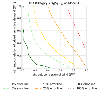
Figure 12: Isolines showing the average absolute percentage error of the point estimator as a function of the structural autocorrelation of wind (instrument) and the structural autocorrelation $\beta^{B1}$ of the price-insensitive demand (dependent variable) for estimator $\#3$. For the simulations, we divide both axes into ten equidistantly spaced autocorrelation coefficients between 0 and 1 each, based on which we run $20$ simulations with five years of data $(T=43,800)$.

In Section 4, we further argue that knowing the observed level of autocorrelation of demand, e.g., obtained by analyzing the (partial) autocorrelation function, does not suffice to correct the estimation bias: the observed autocorrelation of the demand function is associated with different levels of error for the naive IV estimator $\text{CIV}(W_{t}|P_{t}\to D_{t}|\emptyset)$ (see Figure 7). Figure 13 extends the same analysis to estimator $\#3$, which conditions on past demand. As expected from the theory, if the estimation model matches the data generation process, the estimator is unbiased regardless of the observed level of autocorrelation. However, under model misspecification, the same observed level of autocorrelation can be associated with percentage errors ranging from $-300$ MW/(EUR/MWh) to $200$ MW/(EUR/MWh).

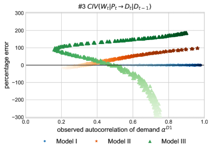
Figure 13: The percentage error of the CIV estimator $\#3$ is shown as a function of the observed autocorrelation of demand $\alpha^{D1}$. In each simulation we vary the structural dependencies: In Models I and II, the strengths of the structural autocorrelations, $\beta^{D1}$ and $\beta^{B1}$, are both varied between $-0.25$ and $0.99$. In Model III, $\beta^{P1}$ is varied between $-250$ MW/(EUR/MWh) and $250$ MW/(EUR/MWh). The color intensity increases in tandem with the aforementioned ranges. For each model, $400$ simulations were conducted, with a sample period of five years $(T=43,800)$.

C.2 Additional indicator plots for Model II and Model III

In Section 4, we have compared the statistical performance of estimators $\#2$, $\#8$ and $\#4$ on data generated from Model I. Figure 14 and Figure 15 compare the performances on data generated by Models II and III, respectively. As expected from theory, all estimators maintain coverage regardless of sample size. Estimator $\#8$ tends to have a smaller absolute percentage error and smaller confidence intervals.

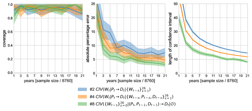
Figure 14: The performance of valid CIV estimators based on the indicators (a) coverage, (b) percentage error, and (c) length of the confidence interval for Model II at different sample sizes. The shaded areas represent the $95\%$ confidence interval for the indicators. For each sample size, $50$ simulations were run. For data generation, the parameters of the demand equation (5) are set to $\beta^{P}=-100$ MW/(EUR/MWh) and $\beta^{B1}=0.9$.

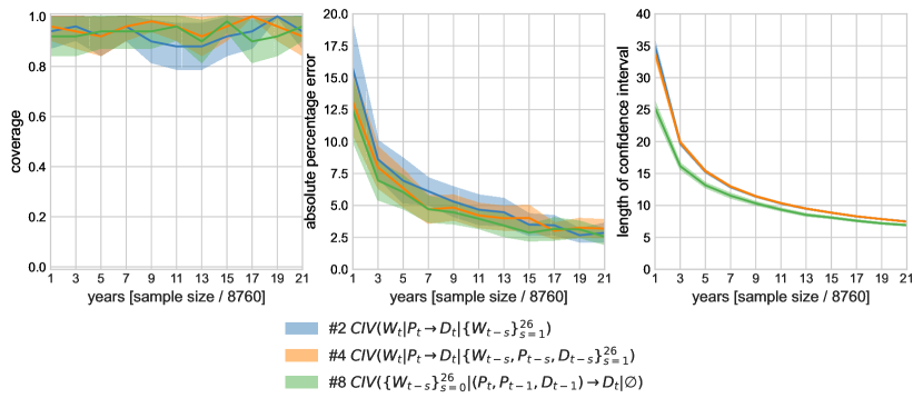
Figure 15: The performance of valid CIV estimators based on the indicators (a) coverage, (b) percentage error, and (c) length of the confidence interval for Model III at different sample sizes. The shaded areas represent the 95% confidence interval for the indicators. For each sample size, $50$ simulations were run. For data generation, the parameters of the demand equation (8) are set to $\beta^{P}=-100$ MW/(EUR/MWh) and $\beta^{P1}=+50$ MW/(EUR/MWh).

C.3 Divergence between CIV estimates for simulated data

In Section 3, we have argued that non-overlapping confidence intervals of presumably valid estimators should lead to model rejection (see also Figure 5 for data from Model I). Figures 16 and 17 show the corresponding patterns of CIV estimators for Model II and Model III, respectively. The table to the right of the figures shows which estimators are valid according to the CIV criteria.

For Model II (Figure 16), the estimators with a checkmark in column II are valid, and the confidence intervals of the corresponding estimators overlap. As done by estimator $\#3$, conditioning on lagged demand generally induces a bias as the estimator conditions on a collider. For Model II, the estimator $\#7$ is a special case: Based on the CIV criteria alone, the estimator is invalid. The estimated effect $P_{t}\to D_{t}$ is nevertheless close to the real effect.

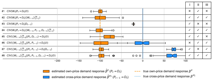
Figure 16: CIV estimates of the demand response $\hat{\beta}^{P}$ when the simulated data does not exhibit structural autocorrelation of demand (Model II, see Figure 3 (left)). The slope of the price-sensitive demand $\beta^{P}$ is set to $-100$ MW/(EUR/MWh), and the autocorrelation coefficient of the non-sensitive demand is set to $\beta^{B1}=0.9$.

The pattern of estimators we observed in Figure 17 is also consistent with the expectation given the Model III assumption. If one were to assume Model III, the researcher does not see much evidence of rejecting that model assumption. However, if, for example, she were to incorrectly assume Model I, there is evidence that this assumption is false (see, e.g., estimators $\#2$ and $\#3$).

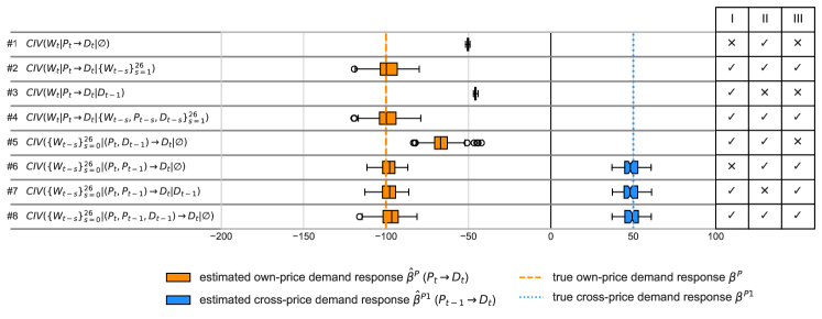
Figure 17: CIV estimates of the demand response $\hat{\beta}^{P}$ when the simulated data represents a cross-price response (Model III, see Figure 3 (right)). The true effect is $\beta^{P}=-100$ MW/(EUR/MWh), and the cross-price elasticity is $\beta^{P1}=+50$ MW/(EUR/MWh), representing substitution. According to theory (see Table 1), the estimators in column III should be consistent, and the simulation results support this. In this model, the validity of the estimators extends to both effects: A valid strategy recovers both the own-price response $\hat{\beta}^{P}$ and the cross-price response $\hat{\beta}^{P1}$.

Appendix D Additional information on Section 5

D.1 Data

We now describe in more detail the data used in the application. The main variables are electricity load (MW), electricity price (€/MWh), and, for the instrument, wind generation (MW, including both onshore and offshore generation), all obtained from [15], the European Network of Transmission System Operators for Electricity. ENTSO-E’s measurement and reporting of variables is bidding zone-specific. Since October 1, 2018, the bidding zone includes the territory of Germany and Luxembourg. Previously, it also included the territory of Austria. The data used in our analysis spans from November 1st, 2017, to December 31st, 2020.

In addition to the main variables, several control series are incorporated into the analysis. If the data exists at a daily frequency, we assume the same value for every hour of the day.

• at hourly frequency:

  • solar PV power generation (from [15])

  • surface temperature data for Germany from NASA’s MERRA-2 [20], transformed according to Eurostat’s methodology [16].

• at daily frequency, all from [30]:

  • price of emissions allowances (EUA yearly futures)

  • coal prices (API 2 CIF ARA ARGUS-McCloskey futures)

  • natural gas price (Dutch TTF futures)

Public holidays and school holidays are two variables constructed as indices based on the fraction of the German population affected by a holiday on a given day, using data from the Federal Statistical Office of Germany (Statistisches Bundesamt Deutschland) for the population by state [14], public holiday dates from Python’s ’holidays‘ package [36], and school holiday dates from [18]. However, holidays common to the whole country and resulting in a value of holiday${}_{t}=1$ (e.g., Easter, Christmas, and the Day of German Unity on October 3rd) are dropped from the dataset. The largest observed value strictly smaller than one equals $0.644$ (three days) and $0.568$ (four days).

We also include the following covariates: sunlight, indicating whether at a given hour of the year, it is day (1) or night (0) at the geographic center of Germany (at 51°09’ N, 10°26’ E) using Python’s ’suntime‘ package [53]; hour of the week (one-hot encoding, 167 variables), month of the year (one-hot encoding, 11 variables), and year (one-hot encoding, four variables).

Figure 18 shows the autocorrelation and partial autocorrelation plots of the instrument and the electricity load after controlling for the control variables. We observe a significant autocorrelation, which is most pronounced for lags 1 and 2 but extends to up to 50 lags, corresponding to more than three days.

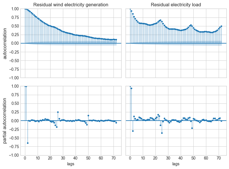
Figure 18: Autocorrelation function (above) and partial autocorrelation function (below) of the residuals of the instrumental time series wind power generation (left), and the residuals of the dependent variable German electricity demand (right). In all four cases, we first regress the original data on the covariates and then obtain the autocorrelation of the residual time series.

D.2 Sensitivity analysis for the price elasticity of German electricity demand

In Section 5, we assume a homogeneous elasticity across hours. However, structurally different consumers may be active across different hours of the day. In particular, one may expect different consumers during peak and off-peak hours. They could either have different elasticities, or they could also have different dynamic behavior. We split the data into two periods and perform the same analysis as in Section 5 on each of the splits: on-peak in Figure 19 and off-peak in Figure 20. The magnitudes of the elasticity estimates (log-log) and the demand response (linear) are comparable. However, the pattern of the estimates is different in the two different splits. This suggests that nighttime consumption has different dynamics than daytime consumption. Given the observed pattern of estimators, we further have to reject all three proposed simple models. This calls for carefully considering the model dynamics if one wants to delve deeper into how electricity consumers respond to a high-frequency price signal.

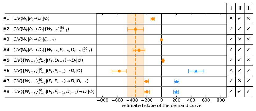
Figure 19: Own-price elasticity of on-peak German electricity demand, obtained from the CIV estimators given in Table 1 in linear specification (top) and log-log specification (bottom). The highlighted area corresponds to the confidence interval of estimator $\#2$. The tables on the right are reproductions of Table 1, showing the validity of each strategy under different structural model assumptions. On-peak hours refer to the time between 8:00 and 19:59.

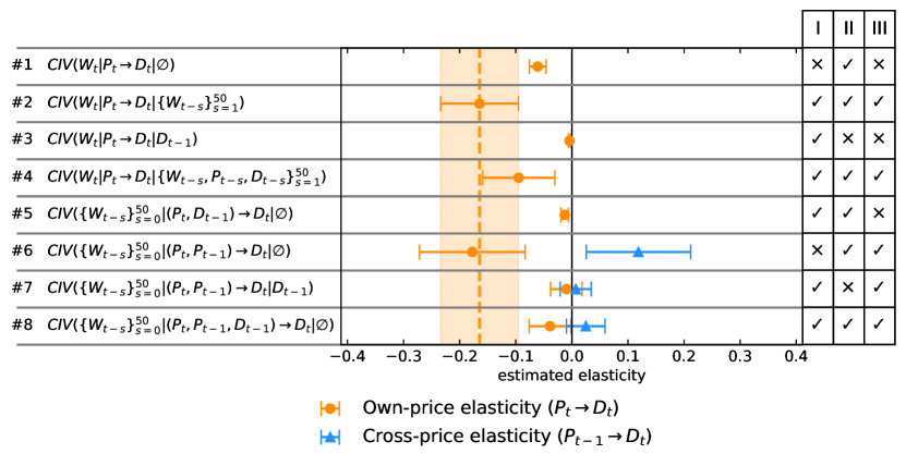
Figure 20: Own-price elasticity of off-peak German electricity demand, obtained from the CIV estimators given in Table 1 in the linear specification (top) and log-log specification (bottom). The highlighted area corresponds to the $95\%$ confidence interval of estimator $\#2$. The tables on the right are reproductions of Table 1, showing the validity of each strategy under different structural model assumptions. Off-peak hours refer to the time between 20:00 and 7:59.

References

- [1] ACER “Decision No 29/2020 on the methodology and assumptions that are to be used in the bidding zone review process and for the alternative bidding zone configurations to be considered”, 2020 URL: https://www.entsoe.eu/network_codes/bzr/
- [2] M.H. Albadi and E.F. El-Saadany “A summary of demand response in electricity markets” In Electric Power Systems Research 78.11, 2008, pp. 1989–1996 DOI: 10.1016/j.epsr.2008.04.002
- [3] J.. Angrist, K. Graddy and G.. Imbens “The Interpretation of Instrumental Variables Estimators in Simultaneous Equations Models with an Application to the Demand for Fish” In The Review of Economic Studies 67.3, 2000, pp. 499–527 URL: https://www.jstor.org/stable/2566964
- [4] J.D. Angrist and J.-S. Pischke “Mostly harmless econometrics: an empiricist’s companion” Princeton: Princeton University Press, 2009
- [5] S. Bongers, P. Forre, J. Peters and J.. Mooij “Foundations of Structural Causal Models with Cycles and Latent Variables” In Annals of Statistics 49.5, 2021, pp. 2885–2915
- [6] W. Bönte, S. Nielen, N. Valitov and T. Engelmeyer “Price elasticity of demand in the EPEX spot market for electricity—New empirical evidence” In Economics Letters 135, 2015, pp. 5–8 DOI: 10.1016/j.econlet.2015.07.007
- [7] S. Borenstein “The Trouble With Electricity Markets: Understanding California’s Restructuring Disaster” In Journal of Economic Perspectives 16.1, 2002, pp. 191–211 DOI: 10.1257/0895330027175
- [8] C. Brito and J. Pearl “Generalized instrumental variables” In Proceedings of the 18th Conference on Uncertainty in Artificial Intelligence (UAI), 2002, pp. 85–93
- [9] C.. Christ “The Cowles Commission’s Contributions to Econometrics at Chicago, 1939-1955” Publisher: American Economic Association In Journal of Economic Literature 32.1, 1994, pp. 30–59 URL: https://www.jstor.org/stable/2728422
- [10] A. Ciarreta, C. Pizarro-Irizar and A. Zarraga “Renewable energy regulation and structural breaks: An empirical analysis of Spanish electricity price volatility” In Energy Economics 88, 2020, pp. 104749 DOI: 10.1016/j.eneco.2020.104749
- [11] P. Cramton, A. Ockenfels and S. Stoft “Capacity Market Fundamentals” In Economics of Energy & Environmental Policy 2.2, 2013 DOI: 10.5547/2160-5890.2.2.2
- [12] S. Cunningham “Causal inference: the mixtape” New Haven, London: Yale University Press, 2021
- [13] P. Dawid “Decision-theoretic foundations for statistical causality” In Journal of Causal Inference 9.1, 2021, pp. 39–77 DOI: doi:10.1515/jci-2020-0008
- [14] Destatistis “Population by nationaly and federal states” https://www.destatis.de/EN/Themes/Society-Environment/Population/Current-Population/Tables/population-by-laender.html. Accessed on 2023-09-17. In Federal Statistical Office, 2023 URL: https://www.destatis.de/EN/Themes/Society-Environment/Population/Current-Population/Tables/population-by-laender.html
- [15] ENTSO-E “ENTSO-E Transparency Platform” https://www.entsoe.eu/network_codes/bzr/. Accessed on 2023-08-14., 2023 URL: https://transparency.entsoe.eu/dashboard/show
- [16] Eurostat “Heating and cooling degree days” https://ec.europa.eu/eurostat/statistics-explained/index.php?title=Heating_and_cooling_degree_days_-_statistics. Accessed on 2023-03-10. In eurostat. Statistics Explained, 2023 URL: https://ec.europa.eu/eurostat/statistics-explained/index.php?title=Heating_and_cooling_degree_days_-_statistics
- [17] N. Fabra, D. Rapson, M. Reguant and J. Wang “Estimating the Elasticity to Real-Time Pricing: Evidence from the Spanish Electricity Market” In AEA Papers and Proceedings 111, 2021, pp. 425–429 DOI: 10.1257/pandp.20211007
- [18] Feiertagskalender “School holidays Germany” https://feiertagskalender.ch/ferien.php?geo=3059&hl=en. Accessed on 2023-09-07. In Feiertagskalender, 2023 URL: https://feiertagskalender.ch/ferien.php?geo=3059&hl=en
- [19] N. Friedman and D. Koller “Being Bayesian about Bayesian Network Structure: A Bayesian Approach to Structure Discovery in Bayesian Networks.” In Machine Learning 50, 2003, pp. 95–125
- [20] Global Modeling And Assimilation Office and S. Pawson “MERRA-2 tavg3_3d_tdt_Np: 3d, 3-Hourly, Time-Averaged, Pressure-Level, Assimilation, Temperature Tendencies V5.12.4” Accessed on 2023-07-12 In NASA Goddard Earth Sciences Data and Information Services Center, 2015 DOI: 10.5067/9NCR9DDDOPFI
- [21] L. Henckel, M. Buttenschoen and M.. Maathuis “Graphical tools for selecting conditional instrumental sets” In Biometrika, 2023, pp. asad066 DOI: 10.1093/biomet/asad066
- [22] D.. Hendry “Dynamic Econometrics” Oxford University PressOxford, 1995 DOI: 10.1093/0198283164.001.0001
- [23] M. Hernan and J. Robins “Causal Inference: What If” Boca Raton: Chapman & Hall/CRC, 2020
- [24] L. Hirth, T.. Khanna and O. Ruhnau “How aggregate electricity demand responds to hourly wholesale price fluctuations” In Energy Economics 135, 2024, pp. 107652 DOI: 10.1016/j.eneco.2024.107652
- [25] P.. Holland “Statistics and Causal Inference” In Journal of the American Statistical Association 81.396, 1986, pp. 945–960
- [26] E. Hosius, J.. Seebass, B. Wacker and J.. Schlüter “The impact of offshore wind energy on Northern European wholesale electricity prices” In Applied Energy 341, 2023, pp. 120910 DOI: 10.1016/j.apenergy.2023.120910
- [27] P. Hünermund and E. Bareinboim “Causal inference and data fusion in econometrics” In The Econometrics Journal, 2023 DOI: 10.1093/ectj/utad008
- [28] G.. Imbens “Potential Outcome and Directed Acyclic Graph Approaches to Causality: Relevance for Empirical Practice in Economics” In Journal of Economic Literature 58.4, 2020, pp. 1129–79
- [29] G.. Imbens and D.. Rubin “Causal Inference for Statistics, Social, and Biomedical Sciences: An Introduction” New York, NY: Cambridge University Press, 2015
- [30] Investing.com “Commodities Prices” https://www.investing.com/commodities. Accessed on 2023-07-23. In Investing.com, 2023 URL: https://www.investing.com/commodities
- [31] Ò. Jordà, M. Schularick and A.. Taylor “Betting the house” In Journal of International Economics 96, 37th Annual NBER International Seminar on Macroeconomics, 2015, pp. S2–S18 DOI: 10.1016/j.jinteco.2014.12.011
- [32] A. Knaut and S. Paulus “When are consumers responding to electricity prices? An hourly pattern of demand elasticity” Number: 2016-7 Publisher: Energiewirtschaftliches Institut an der Universitaet zu Koeln (EWI) In EWI Working Papers, 2017 URL: https://ideas.repec.org//p/ris/ewikln/2016_007.html
- [33] S.. Lauritzen “Graphical Models” New York, NY, USA: Oxford University Press, 1996
- [34] S.. Lauritzen, A.. Dawid, B.. Larsen and H.-G. Leimer “Independence properties of directed markov fields” In Networks 20, 1990, pp. 491–505
- [35] G.. Maniatis and N.. Milonas “The impact of wind and solar power generation on the level and volatility of wholesale electricity prices in Greece” In Energy Policy 170, 2022, pp. 113243 DOI: 10.1016/j.enpol.2022.113243
- [36] M. Montel and A. Yakovets “holidays: Generate and work with holidays in Python”, 2023
- [37] J.L. Montiel Olea and M. Plagborg-Møller “Local Projection Inference Is Simpler and More Robust Than You Think” Publisher: John Wiley & Sons, Ltd In Econometrica 89.4, 2021, pp. 1789–1823 DOI: 10.3982/ECTA18756
- [38] J.L. Montiel Olea, M. Plagborg-Møller, E. Qian and C.K. Wolf “Double Robustness of Local Projections and Some Unpleasant VARithmetic” In National Bureau of Economic Research, Working Paper Series National Bureau of Economic Research, 2024 DOI: 10.3386/w32495
- [39] J. Neyman “On the Application of Probability Theory to Agricultural Experiments. Essay on Principles. Section 9 (translated)” In Statistical Science 5, 1923, pp. 465–480
- [40] J. Pearl “Causality: Models, Reasoning, and Inference” New York, USA: Cambridge University Press, 2009
- [41] J. Pearl and D. Mackenzie “The book of why: the new science of cause and effect” New York: Basic Books, 2020
- [42] J. Peters, S. Bauer and N. Pfister “Causal Models for Dynamical Systems” In Probabilistic and Causal Inference: The Works of Judea Pearl 36 New York, NY, USA: Association for Computing Machinery, 2022, pp. 671–690 URL: https://doi.org/10.1145/3501714.3501752
- [43] J. Peters, P. Bühlmann and N. Meinshausen “Causal inference using invariant prediction: identification and confidence intervals” In Journal of the Royal Statistical Society: Series B (with discussion) 78.5, 2016, pp. 947–1012
- [44] J. Peters, D. Janzing and B. Schölkopf “Causal Inference on Time Series using Structural Equation Models” In Advances in Neural Information Processing Systems 26 (NeurIPS) Curran Associates, Inc., 2013, pp. 585–592
- [45] J. Peters, D. Janzing and B. Schölkopf “Elements of Causal Inference: Foundations and Learning Algorithms” Cambridge, MA, USA: MIT Press, 2017
- [46] M. Plagborg-Møller and C.. Wolf “Local Projections and VARs Estimate the Same Impulse Responses” In Econometrica 89.2, 2021, pp. 955–980 DOI: 10.3982/ECTA17813
- [47] V.. Ramey and S. Zubairy “Government Spending Multipliers in Good Times and in Bad: Evidence from US Historical Data” Publisher: The University of Chicago Press In Journal of Political Economy 126.2, 2018, pp. 850–901 DOI: 10.1086/696277
- [48] T. Richardson “Markov properties for acyclic directed mixed graphs” In Scandinavian Journal of Statistics 30.1 Wiley Online Library, 2003, pp. 145–157
- [49] D.. Rubin “Causal inference using potential outcomes” In Journal of the American Statistical Association 100, 2005, pp. 322–331
- [50] K. Sheppard and al. “bashtage/linearmodels: Release 6.0” https://zenodo.org/doi/10.5281/zenodo.10981685 [object Object], 2024 DOI: 10.5281/ZENODO.10981685
- [51] P. Spirtes, C. Glymour and R. Scheines “Causation, Prediction, and Search” MIT Press, 2000
- [52] J.. Stock and M.. Watson “Identification and Estimation of Dynamic Causal Effects in Macroeconomics Using External Instruments” In The Economic Journal 128.610, 2018, pp. 917–948 DOI: 10.1111/ecoj.12593
- [53] K. Stopa “suntime: Simple sunset and sunrise time calculation python library.” https://github.com/SatAgro/suntime, 2019 URL: https://github.com/SatAgro/suntime
- [54] N. Thams, R. Søndergaard, S. Weichwald and J. Peters “Identifying Causal Effects using Instrumental Time Series: Nuisance IV and Correcting for the Past” In Journal of Machine Learning Research (accepted)” arXiv, 2022 arXiv: http://arxiv.org/abs/2203.06056
- [55] J. Tinbergen “Econometric Business Cycle Research” Publisher: [Oxford University Press, Review of Economic Studies, Ltd.] In The Review of Economic Studies 7.2, 1940, pp. 73–90 DOI: 10.2307/2967472
- [56] T.. Verma and J. Pearl “Equivalence and synthesis of causal models” In Proceedings of the 6th Annual Conference on Uncertainty in Artificial Intelligence (UAI), 1991, pp. 255–270
- [57] K. Webel “A Review of Some Recent Developments in the Modelling and Seasonal Adjustment of Infra-Monthly Time Series” In SSRN Electronic Journal, 2022 DOI: 10.2139/ssrn.4201921
- [58] H… Wold “Econometric model building; essays on the causal chain approach” Amsterdam: North-Holland Pub. Co., 1964 URL: https://search.library.wisc.edu/catalog/999539203202121
- [59] P.. Wright “The Tariff on Animal and Vegetable Oils”, Investigations in International Commercial Policies New York, NY: Macmillan, 1928