Optimality of a barrier strategy in a spectrally negative Lévy model with a level-dependent intensity of bankruptcy

Abstract.

We consider de Finetti’s stochastic control problem for a spectrally negative Lévy process in an Omega model. In such a model, the (controlled) process is allowed to spend time under the critical level but is then subject to a level-dependent intensity of bankruptcy. First, before considering the control problem, we derive some analytical properties of the corresponding Omega scale functions. Second, we prove that exists a barrier strategy that is optimal for this control problem under a mild assumption on the Lévy measure. Finally, we analyse numerically the impact of the bankruptcy rate function on the optimal strategy.

1. Introduction

The stochastic control problem concerned with the maximization of dividend payments in a model based on a (general) spectrally negative Lévy process (SNLP) has attracted a lot of research interest since the papers of Avram, Palmowski & Pistorius [avram-palmowski-pistorius_2007] and Loeffen [loeffen_2008]. In that problem, a dividend strategy is said to be optimal if it maximises the expected present value of dividend payments made up to the ruin time, which is a standard first-passage time. The recent developments in Parisian fluctuation theory for SNLPs have inspired the use of a Parisian ruin time as the termination time in that control problem; see, e.g., [czarna-palmowski_2014, renaud2019, xu-et-al_2021, locas-renaud_2024b]. In particular, when using an exponential Parisian ruin time, i.e., with exponentially distributed delays, it has been possible to formulate a sufficient condition, namely on the Lévy measure, under which one can guarantee that a barrier strategy is optimal; see [renaud2019]. This sufficient condition, for the optimality of a barrier strategy, dates back to [loeffen-renaud_2010] in the classical version of the problem. It was proved that this condition on the Lévy measure guarantees the convexity of $W_{q}^{\prime}$, which is the derivative of the $q$-scale function $W_{q}$ of the corresponding SNLP; here, $q$ is the time-preference factor in the maximization problem. This convexity property is needed in particular to characterize the optimal barrier level. Then, in [renaud2019], it was proved that this convexity property was transferable to another scale function, namely $Z_{q}(\cdot,\Phi(p+q))$, which is at the core of the problem when Parisian ruin at rate $p$ is used as the termination time.

It is now well known that a Parisian first-passage time with exponential delays has connections with the distribution of certain occupation times of the underlying process; see, e.g., [landriault-et-al_2011]. In that paper, there is also a connection with so-called Omega models, which were introduced in [albrecher-et-al_2011b, gerber-et-al_2012]. In such a model, and in the spirit of Parisian ruin aiming at making a distinction between default and bankruptcy, the probability of bankruptcy is a function of the surplus level. More precisely, given a bankruptcy rate function $\omega(\cdot)$, if the surplus is at a level $x<0$, then the corresponding rate of bankruptcy is given by $\omega(x)$; a full definition is provided in Definition 2.1. This concept of level-dependent bankruptcy was made rigorous for SNLPs by Li & Palmowski [li-palmowski_2018]. Indeed, they provided a general level-dependent notion of discounting for SNLPs, in the spirit of the connection between exponential Parisian ruin and occupation times. In fact, exponential Parisian ruin at rate $p$ corresponds to the bankruptcy rate function $\omega(x)=p\mathbf{1}_{(-\infty,0)}(x)$. In [li-palmowski_2018], all fluctuation identities with level-dependent discounting are expressed in terms of some generalised scale functions, also called Omega scale functions. These functions are defined implicitly as the solutions of Volterra integral equations; see Equation (6) below.

1.1. Stochastic model

In this paper, we study the problem of dividend maximization for a SNLP. Henceforth, consider a filtered probability space $\left(\Omega,\mathcal{F},\left\{\mathcal{F}_{t},t\geq 0\right\},\mathbb{P}\right)$ such that $\mathcal{F}_{\infty}:=\bigvee_{t\geq 0}\mathcal{F}_{t}\subsetneq\mathcal{F}$, where $\bigvee_{t\geq 0}\mathcal{F}_{t}$ is the smallest $\sigma$-algebra containing $\mathcal{F}_{t}$ for all $t\geq 0$. Let $X=\left\{X_{t},t\geq 0\right\}$ be a SNLP (adapted to the filtration $\left\{\mathcal{F}_{t},t\geq 0\right\}$) with Laplace exponent

$$\psi(\theta)=\gamma\theta+\frac{1}{2}\sigma^{2}\theta^{2}+\int^{\infty}_{0}\left(\mathrm{e}^{-\theta z}-1+\theta z\mathbf{1}_{(0,1]}(z)\right)\nu(\mathrm{d}z),\quad\theta\geq 0,$$

where $\gamma\in\mathbb{R}$ and $\sigma\geq 0$, and where $\nu$ is a $\sigma$-finite measure on $(0,\infty)$, called the Lévy measure of $X$, satisfying

$$\int^{\infty}_{0}(1\wedge x^{2})\nu(\mathrm{d}x)<\infty.$$

The corresponding scale functions $\left\{W_{p},p\geq 0\right\}$ are then given by

$$\int_{0}^{\infty}\mathrm{e}^{-\theta x}W_{p}(x)\mathrm{d}x=\left(\psi(\theta)-p\right)^{-1},$$

for all $\theta>\Phi(p)=\sup\left\{\lambda\geq 0\colon\psi(\lambda)=p\right\}$. For more details on SNLPs and scale functions, see, e.g., [kuznetsov-et-al_2012, kyprianou_2014].

In what follows, we will use the following notation: the law of $X$ when starting from $X_{0}=x$ is denoted by $\mathbb{P}_{x}$ and the corresponding expectation by $\mathbb{E}_{x}$. We write $\mathbb{P}$ and $\mathbb{E}$ when $x=0$.

1.2. Optimisation problem

Let $X$ be the underlying wealth (cash, surplus) process. A control dividend strategy $\pi$ is represented by a non-decreasing, right-continuous and adapted stochastic process $L^{\pi}=\left\{L^{\pi}_{t},t\geq 0\right\}$ such that $L^{\pi}_{0-}=0$, where $L^{\pi}_{t}$ represents the cumulative amount of dividends made/paid up to time $t$ under this control strategy. For a given strategy $\pi$, the corresponding controlled process $U^{\pi}=\left\{U^{\pi}_{t},t\geq 0\right\}$ is defined by $U^{\pi}_{t}=X_{t}-L^{\pi}_{t}$. A strategy is said to be admissible if $0\leq L_{t}^{\pi}-L_{t-}^{\pi}\leq U_{t-}\vee 0$, for all $t$. Let $\Pi$ be the set of admissible strategies.

In order to define the termination/bankruptcy time of interest, let us fix a bankruptcy rate function $\omega\colon\mathbb{R}\to[0,\infty)$, that is roughly speaking a non-negative and non-increasing function having support in $(-\infty,0]$; a full definition is provided in Definition 2.1. Correspondingly, we define the following termination time associated with $\omega(\cdot)$: for $\pi\in\Pi$, set

$$\sigma^{\pi}_{\omega}=\inf\left\{t>0\colon\int_{0}^{t}\omega(U^{\pi}_{s})\mathrm{d}s>\mathbf{e}_{1}\right\},$$ (1)

where $\mathbf{e}_{1}$ is an independent random variable following the exponential distribution with unit mean.

Finally, fix a time-preference/discount rate $q>0$. The performance function associated to an arbitrary $\pi\in\Pi$ is defined by

$$v_{\pi}(x)=\mathbb{E}_{x}\left[\int_{0}^{\sigma^{\pi}_{\omega}}\mathrm{e}^{-qt}\mathrm{d}L^{\pi}_{t}\right],\quad x\in\mathbb{R}.$$

The goal is to compute

$$v_{\ast}(x)=\sup_{\pi\in\Pi}v_{\pi}(x),\quad x\in\mathbb{R},$$

the (optimal) value function of this control problem by finding an optimal strategy $\pi_{\ast}\in\Pi$, i.e., an admissible strategy such that

$$v_{\pi_{\ast}}(x)=v_{\ast}(x),\quad x\in\mathbb{R}.$$

More precisely, in this paper, we find a sufficient condition on the Lévy measure for a barrier strategy (see Section 3.2) to be optimal, in the spirit of the existing literature on the maximization of dividends in a SNLP model that has followed since [loeffen_2008]. See Theorem 3.1 below.

1.3. Contributions and organisation of the paper

As alluded to above, our problem is a generalization of the one studied in [renaud2019], which was itself an asymptotic generalization of the classical problem studied in [loeffen_2008, loeffen-renaud_2010]. It turns out that no extra condition on the model is required to guarantee that a barrier strategy is optimal, even with this more general definition of bankruptcy; compare Theorem 3.1 below with Theorem 1.1 in [loeffen-renaud_2010] and Theorem 1 in [renaud2019].

To prove our main result, we need to study Omega scale functions beyond what is done in [li-palmowski_2018]. More precisely, we derive semi-explicit expressions for those Omega scale functions by solving the corresponding Volterra equations. Finally, we are able to identify differentiability and convexity properties of those scale functions, in the spirit of those for classical scale functions (see Theorem 2.1). Those analytical properties are needed in the verification step of our solution to this control problem. It must be pointed out that these results about Omega scale functions are of independent interest and improve upon the theory developed in [li-palmowski_2018]. The same methodology would apply to the other scale functions studied in that paper, for example to $\mathcal{W}^{\omega}$.

The rest of this paper is structured as follows. In the next section, the definitions of a discounting intensity and then of a bankruptcy rate function are given, and a detailed analysis of Omega scale functions is provided. In Section 3, we come back to our optimisation problem: first, we compute the performance function of an arbitrary barrier strategy, and then we prove that one of these is optimal for our control problem (Theorem 3.1). Section 4 contains the proof of this main result. The last section contains numerical experiments illustrating the sensitivity of the optimal strategy and the value function with respect to the bankruptcy rate function. The proof of Lemma 2.1 is given in the Appendix.

2. Scale functions

In the rest of this paper, we make the following standing assumption:

Assumption 2.1.

If the paths of $X$ are of bounded variation (BV), then the Lévy measure is assumed to be absolutely continuous with respect to Lebesgue measure.

As a consequence of this assumption, we have that the scale function $W_{p}$ is continuously differentiable on $(0,\infty)$, for any $p\geq 0$; see, e.g., [kuznetsov-et-al_2012].

Recall that $q$ is the discount rate. Since [avram-et-al_2007, loeffen_2008], it has been widely known that the $q$-scale function $W_{q}$ is an essential object in the study of the optimal dividends problem with classical ruin. When exponential Parisian ruin is considered, as in [renaud2019], a second family of scale functions is needed. If Parisian ruin occurs at rate $\phi>0$, i.e., if $\omega(x)=\phi\mathbf{1}_{(-\infty,0)}(x)$, then $Z_{q}(\cdot;\Phi(\phi+q))$ is the scale function of interest. In general, for fixed $0<r<s$, define, for each $x\in\mathbb{R}$,

$$Z_{r}(x;\Phi(s))=\mathrm{e}^{\Phi(s)x}\left(1-(s-r)\int_{0}^{x}\mathrm{e}^{-\Phi(s)y}W_{r}(y)\mathrm{d}y\right)\\ =(s-r)\int_{0}^{\infty}\mathrm{e}^{-\Phi(s)y}W_{r}(x+y)\mathrm{d}y,$$ (2)

where for $x\leq 0$, we have $Z_{q}(x;\Phi(s))=\mathrm{e}^{\Phi(s)x}$. In particular, we have $Z_{q}(x;\Phi(\phi+q))=\phi\int_{0}^{\infty}\mathrm{e}^{-\Phi(\phi+q)y}W_{q}(x+y)\mathrm{d}y$.

Before defining the scale function of interest in our context, let us give two identities involving the scale functions defined so far.

Lemma 2.1.

For real numbers $a\leq b<x$, we have

$$\int_{a}^{x}W_{p}(x-y)W_{r}(y-a)\mathrm{d}y=\frac{W_{r}(x-a)-W_{p}(x-a)}{r-p}$$ (3)

and, if $s>\max\{p,r\}$, we have

$$\int_{a}^{x}W_{p}(x-y)Z_{r}(y-a;\Phi(s))\mathrm{d}y=\frac{Z_{r}(x-a;\Phi(s))-Z_{p}(x-a;\Phi(s))}{r-p}.$$ (4)

To the best of our knowledge, a version of the identity in (3) first appeared in Lemma 3 of [pistorius_2004] in which its proof is based on a well-known power series expansion of the $p$-scale function $W_{p}$. Another proof, based on Laplace transforms, is provided in [loeffen-et-al_2014]. The identity in (4) first appeared in Lemma 4.1 of [albrecher-et-al_2016], in a slightly modified version; its proof is based on Laplace transforms. In Appendix A, we provide an arguably simpler and shorter proof.

2.1. Discounting intensity

In the next section, we will define and study a generalised scale function associated to a given discounting intensity. Now, let us provide a full definition.

Definition 2.1.

We say that $\omega\colon\mathbb{R}\to[0,\infty)$ is a discounting intensity if:

1. it is non-increasing;

2. it is ultimately constant, i.e., there exist $a\in(-\infty,0]$ and $\phi>0$ for which $\omega(x)=\phi$ for all $x\in(-\infty,a)$, and there exists $\rho\in[0,\omega(0-))$ such that $\omega(x)=\rho$ for all $x\in[0,\infty)$;

3. it is piecewise continuous, i.e., there exists a finite partition $\{a_{1},a_{2},\dots,a_{n},a_{n+1}\}$ of $[a,0]$ given by $a=a_{1}<a_{2}<\cdots<a_{n}\leq a_{n+1}=0$ and such that:

   1. $\omega$ is continuous on each sub-interval $(a_{k},a_{k+1})$ for $k\in\{1,2,\cdots,n\}$;

   2. if $n\geq 2$, then $\omega(a_{k}-)>\omega(a_{k}+)$ for each $k\in\{2,\cdots,n\}$.

In particular, in an Omega model, we say that $\omega$ is a bankruptcy rate function if it is a discounting intensity with $\rho=0$.

Note that the assumption of being ultimately constant comes from Section 2.4 in [li-palmowski_2018].

As opposed to other elements in the partition, a discounting intensity might or might not have jumps at $a$ and $0$. More precisely, we have $\phi=\omega(a-)\geq\omega(a+)$ and $\omega(0-)\geq\rho=\omega(0)$. Thus, if $\omega$ is continuous on $(-\infty,0)$, then $n=1$ and $a\leq 0$ and thus the only possible discontinuity point is now at $0$. This is the case for example if $\omega(x)=\phi\mathbf{1}_{(-\infty,0)}(x)+\rho\mathbf{1}_{[0,\infty)}(x)$. However, it is possible for $\omega$ to be continuous on $\mathbb{R}$. For example,

$$\omega(x)=\phi\mathbf{1}_{(-\infty,-\phi)}(x)-x\mathbf{1}_{[-\phi,0)}(x)$$

is a continuous discounting intensity/bankruptcy rate function.

An important family of discounting intensities/bankruptcy rate functions is given by piecewise constant functions. For example, for a partition $-\infty=a_{0}<a_{1}<\dots<a_{n}<0=a_{n+1}$ and decreasing rates given by $\phi=p_{0}>p_{1}>\dots>p_{n}>0$, we can define

$$\omega(x)=\sum_{i=1}^{n+1}p_{i-1}\mathbf{1}_{[a_{i-1},a_{i})}(x)=p_{0}\mathbf{1}_{(-\infty,a_{1})}(x)+p_{1}\mathbf{1}_{[a_{1},a_{2})}(x)+\dots+p_{n}\mathbf{1}_{[a_{n},a_{n+1})}(x),$$ (5)

where, for simplicity, we used the notation $[a_{0},a_{1}):=(-\infty,a_{1})$. Intuitively speaking, the function given in (5) is such that the rate $p_{i}$ is applied when the process is in the interval $[a_{i},a_{i+1})$. As the process goes deeper into the red zone, since we have $p_{i}<p_{i-1}$, the discouting rates increase.

Remark 2.1.

In an Omega model, a piecewise constant bankruptcy rate function yields a termination time that is already significantly more general than a Parisian ruin time with exponential delays. Indeed, Parisian ruin with exponential rate $\phi>0$ corresponds to the bankruptcy rate function $\omega(x)=\phi\mathbf{1}_{(-\infty,0)}(x)$.

2.2. Omega scale functions

For the control problem under study, we need a generalization of both $W_{q}(\cdot)$ and $Z_{q}(\cdot;\Phi(\phi+q))$. A theory of scale functions based on a discounting intensity $\omega$ has been developed in [li-palmowski_2018]. In that paper, the $\omega$-scale function $\mathcal{H}^{\omega}\colon\mathbb{R}\to\mathbb{R}$ is defined as the solution of the following functional equation:

$$\mathcal{H}^{\omega}(x)=\mathrm{e}^{\Phi(\phi)(x-a)}+\int_{a}^{x}W_{\phi}(x-y)(\omega(y)-\phi)\mathcal{H}^{\omega}(y)\mathrm{d}y,\quad x\in\mathbb{R}.$$ (6)

See Lemma 2.1 and Section 2.4 in [li-palmowski_2018] for more details.

In the above definition and in what follows, it is assumed that, for any integrable function $f$, if $a\geq b$ then $\int_{a}^{b}f(x)\mathrm{d}x=0$. In general, by $\int_{a}^{b}$ we mean $\int_{[a,b)}$.

Remark 2.2.

Note that (6) does not appear verbatim in [li-palmowski_2018]. We have performed a translation in Equations (2.22)-(2.23) of [li-palmowski_2018] to obtain (6). This modification is needed to be in agreement with our definition of a discounting intensity.

First, let us provide a continuum of alternate functional equations for the definition of the $\omega$-scale function $\mathcal{H}^{\omega}$.

Lemma 2.2.

For a fixed $p\geq 0$, we have

$$\mathcal{H}^{\omega}(x)=Z_{p}(x-a;\Phi(\phi))+\int_{a}^{x}W_{p}(x-y)(\omega(y)-p)\mathcal{H}^{\omega}(y)\mathrm{d}y,\quad x\in\mathbb{R}.$$ (7)

Proof.

Using the definition of $\mathcal{H}^{\omega}$ as given by (6), we can write

$$\int_{a}^{x}W_{p}(x-y)\mathcal{H}^{\omega}(y)\mathrm{d}y\\ =\int_{a}^{x}\mathrm{e}^{\Phi(\phi)(y-a)}W_{p}(x-y)\mathrm{d}y+\int_{a}^{x}W_{p}(x-y)\left[\int_{a}^{y}W_{\phi}(y-z)(\omega(z)-\phi)\mathcal{H}^{\omega}(z)\mathrm{d}z\right]\mathrm{d}y\\ =\int_{0}^{x-a}\mathrm{e}^{\Phi(\phi)(x-y-a)}W_{p}(y)\mathrm{d}y+\int_{a}^{x}(\omega(z)-\phi)\mathcal{H}^{\omega}(z)\left[\int_{z}^{x}W_{p}(x-y)W_{\phi}(y-z)\mathrm{d}y\right]\mathrm{d}z,$$

in which, by Lemma (2.1), we have

$$\int_{z}^{x}W_{p}(x-y)W_{\phi}(y-z)\mathrm{d}y=\frac{W_{p}(x-z)-W_{\phi}(x-z)}{p-\phi}.$$

Using (6) to replace $\int_{a}^{x}W_{\phi}(x-y)(\omega(y)-\phi)\mathcal{H}^{\omega}(y)\mathrm{d}y$ by $\mathcal{H}^{\omega}(x)-\mathrm{e}^{\Phi(\phi)(x-a)}$ and identifying $Z_{p}(x-a;\Phi(\phi))$, we can further write

$$(p-\phi)\int_{a}^{x}W_{p}(x-y)\mathcal{H}^{\omega}(y)\mathrm{d}y\\ =Z_{p}(x-a;\Phi(\phi))-\mathcal{H}^{\omega}(x)+\int_{a}^{x}W_{p}(x-y)(\omega(y)-\phi)\mathcal{H}^{\omega}(y)\mathrm{d}y.$$

The result follows. ∎

Note that, in the last lemma, if $p=\phi$ then $Z_{p}(y;\Phi(\phi))=\mathrm{e}^{\Phi(\phi)y}$ and we recover (6).

Remark 2.3.

Of course, $\mathcal{H}^{\omega}$ is independent of the arbitrarily chosen value of $p$. Later, when solving the control problem, we will make an appropriate choice for $p$.

Second, let us apply a methodology based on Picard iterations. Note that this methodology has been used also in [czarna-et-al_2019] for a similar but different situation. Fix an arbitrary $p\in[0,\rho]$. For $x,y\in\mathbb{R}$, set the kernel $K(x,y)=W_{p}(x-y)(\omega(y)-p)$ and then define $K_{1}(x,y)=K(x,y)$ and, for each $m\geq 2$, define

$$K_{m}(x,y)=\int_{y}^{x}K_{1}(x,z)K_{m-1}(z,y)\mathrm{d}z.$$ (8)

Note that, for each $m\geq 1$, if $x<y$ then $K_{m}(x,y)=0$.

Now, for each $m\geq 1$, define $\overline{K}_{m}(x,y)=\sum_{i=1}^{m}K_{i}(x,y)$ and then define

$$\mathcal{H}_{m}(x)=Z_{p}(x-a;\Phi(\phi))+\int_{a}^{x}\overline{K}_{m}(x,y)Z_{p}(y-a;\Phi(\phi))\mathrm{d}y.$$ (9)

Lemma 2.3.

For $m\geq 1$, we have

$$\mathcal{H}_{m}(x)=Z_{p}(x-a;\Phi(\phi))+\int_{a}^{x}K(x,y)\mathcal{H}_{m-1}(y)\mathrm{d}y,\quad x\in\mathbb{R},$$ (10)

where $\mathcal{H}_{0}(x):=Z_{p}(x-a;\Phi(\phi))$.

Proof.

Let us prove the result by induction. If $m=1$, then the result coincides with the definition of $\mathcal{H}_{m}$ given in (9). Assume the result in (10) is true for an arbitrary $m\geq 1$.

Clearly, by the definition of $\mathcal{H}_{m+1}$ given in (9), we can write

$$\mathcal{H}_{m+1}(x) =\mathcal{H}_{m}(x)+\int_{a}^{x}K_{m+1}(x,y)Z_{p}(y-a;\Phi(\phi))\mathrm{d}y$$

$$=Z_{p}(x-a;\Phi(\phi))+\int_{a}^{x}K(x,y)\mathcal{H}_{m-1}(y)\mathrm{d}y$$

$$\qquad+\int_{a}^{x}\left[\int_{y}^{x}K(x,z)K_{m}(z,y)\mathrm{d}z\right]Z_{p}(y-a;\Phi(\phi))\mathrm{d}y,$$

where, in the second equality, we used the induction hypothesis and the following equivalent definition of $K_{m+1}$:

$$K_{m+1}(x,y)=\int_{y}^{x}K_{m}(x,z)K_{1}(z,y)\mathrm{d}z.$$

The latter is easy to prove and left to the reader.

So, to prove the result, it suffices to verify that

$$\int_{a}^{x}K(x,y)\mathcal{H}_{m}(y)\mathrm{d}y\\ =\int_{a}^{x}K(x,y)\mathcal{H}_{m-1}(y)\mathrm{d}y+\int_{a}^{x}\left[\int_{y}^{x}K(x,z)K_{m}(z,y)\mathrm{d}z\right]Z_{p}(y-a;\Phi(\phi))\mathrm{d}y.$$

It follows from the fact that

$$\int_{a}^{x}K(x,y)\left[\mathcal{H}_{m}(y)-\mathcal{H}_{m-1}(y)\right]\mathrm{d}y =\int_{a}^{x}K(x,y)\int_{a}^{y}K_{m}(y,z)Z_{p}(z-a;\Phi(\phi))\mathrm{d}z\mathrm{d}y$$

$$=\int_{a}^{x}Z_{p}(z-a;\Phi(\phi))\int_{z}^{x}K(x,y)K_{m}(y,z)\mathrm{d}y\mathrm{d}z.$$

The proof is complete.

∎

Finally, let us define

$$R_{p}(x,y):=\lim_{m\to\infty}\overline{K}_{m}(x,y)=:\sum_{m=1}^{\infty}K_{m}(x,y).$$ (11)

In Lemma 2.4 below, we will prove that it is a well-defined function.

We are ready to state our first main result, which contains a solution to functional equation (6) and some of its analytical properties.

Theorem 2.1.

Fix $p\in[0,\rho]$. The $\omega$-scale function $\mathcal{H}^{\omega}$ is given by

$$\mathcal{H}^{\omega}(x)=Z_{p}(x-a;\Phi(\phi))+\int_{a}^{x}R_{p}(x,y)Z_{p}(y-a;\Phi(\phi))\mathrm{d}y,\quad x\in\mathbb{R}.$$ (12)

Moreover, $\mathcal{H}^{\omega}$ has the following differentiability properties:

1. If $X$ has paths of UBV, then $\mathcal{H}^{\omega}$ is continuously differentiable on $\mathbb{R}$. In addition, if $\sigma>0$, then $\mathcal{H}^{\omega}$ is twice continuously differentiable on $\mathbb{R}\setminus\{a_{1},a_{2},\cdots,a_{n}\}$.

2. If $X$ has paths of BV, then $\mathcal{H}^{\omega}$ is:

   1. continuously differentiable on $\mathbb{R}\setminus\{a_{1},a_{2},\dots,a_{n}\}$ if $\omega(0-)=0$;

   2. continuously differentiable on $\mathbb{R}\setminus\{a_{1},a_{2},\dots,a_{n},a_{n+1}\}$ if $\omega(0-)>0$.

Note that the differentiability properties of $\mathcal{H}^{\omega}$ are reminiscent of those for $W_{p}$, where $p\geq 0$; see, e.g., [kuznetsov-et-al_2012].

2.3. Proof of Theorem 2.1

Let us break down the proof of Theorem 2.1. First, the next lemma completes the methodology started in the previous section.

Lemma 2.4.

Fix $p\in[0,\rho]$. The function $R_{p}$ is well defined. Also, $(\mathcal{H}_{m})_{m\geq 1}$ converges to $\mathcal{H}^{\omega}$ and $\mathcal{H}^{\omega}$ is continuous on $\mathbb{R}$.

Proof.

First, recall that, if $x<y$, then $K_{m}(x,y)=0$ for each $m\geq 1$. Since $\omega$ is bounded, it is easy to show that, for each $m\geq 1$,

$$0\leq K_{m}(x,y)\leq(\phi-p)^{m}W_{p}^{\ast m}(x-y),$$ (13)

where $W_{p}^{\ast m}$ denotes the $m$-fold convolution of $W_{p}$ with itself.

Let us find a (finite) function $\zeta(x,y)$ such that, for each $m\geq 1$,

$$0\leq\sum_{i=1}^{m}K_{i}(x,y)\leq\zeta(x,y).$$ (14)

In this direction, recall from the proof of Lemma 8.3 in [kyprianou_2014] that, for a given $r>0$, we have

$$W_{r+p}(x)=\sum_{k=0}^{\infty}r^{k}W_{p}^{\ast(k+1)}(x),\quad x\geq 0.$$

Therefore, in view of inequality (13), as the majorant function in (14), we can take

$$\zeta(x,y):=(\phi-p)W_{\phi}(x-y).$$

It follows that $R_{p}(x,y)$ is well defined as the limit of $\left(\overline{K}_{m}(x,y)\right)_{m\geq 1}$ and we have $R_{p}(x,y)\leq\zeta(x,y)$.

In order to conclude that $\mathcal{H}_{m}$ also converges to a well-defined limit, all is left to verify is that $\int_{a}^{x}R_{p}(x,y)Z_{p}(y-a;\Phi(\phi))\mathrm{d}y<\infty$. By (4) in Lemma 2.1, we have

$$\int_{a}^{x}\zeta(x,y)Z_{p}(y-a;\Phi(\phi))\mathrm{d}y=(\phi-p)\int_{0}^{x-a}W_{\phi}(x-a-y)Z_{p}(y;\Phi(\phi))\mathrm{d}y\\ =Z_{\phi}(x;\Phi(\phi))-Z_{p}(x;\Phi(\phi)),$$

which is finite.

Finally, we have that $\overline{K}_{m}$ is non-negative for all $m\geq 1$, hence $\mathcal{H}_{m}$ is a non-decreasing sequence of continuous functions. It follows from Dini’s Theorem that $(\mathcal{H}_{m})_{m\geq 1}$ converges uniformly on compact sets of $\mathbb{R}$, and that it converges to

$$\mathcal{H}^{\omega}(x)=Z_{p}(x;\Phi(\phi))+\int_{a}^{x}R_{p}(x,y)Z_{p}(y-a;\Phi(\phi))\mathrm{d}y,\quad x\in\mathbb{R}.$$

We deduce finally that $\mathcal{H}^{\omega}$ is continuous on $\mathbb{R}$.

∎

We are now ready to complete the proof of Theorem 2.1, more precisely the second part of the statement about the differentiability properties of $\mathcal{H}^{\omega}$.

Recall that $a_{1}=a$ and $a_{n+1}=0$. Fix $p\in[0,\rho]$. Then, by Lemma 2.4, we have

$$\mathcal{H}^{\omega}(x)=Z_{p}(x-a;\Phi(\phi))+\int_{a}^{x}R_{p}(x,y)Z_{p}(y-a;\Phi(\phi))\mathrm{d}y,\quad x\in\mathbb{R},$$

as in Equation (12).

First, let us analyse $I(x):=\int_{a}^{x}R_{p}(x,y)Z_{p}(y-a;\Phi(\phi))\mathrm{d}y$. It is easy to verify that, for any $x\in\mathbb{R}$, we have

$$R_{p}(x,x)=W_{p}(0)(\omega(x)-p).$$

Then, applying Leibniz rule, we can write

$$I^{\prime}(x)=K(x,x)Z_{p}(x-a;\Phi(\phi))+\int_{a}^{x}\frac{\partial}{\partial x}R_{p}(x,y)Z_{p}(y-a;\Phi(\phi))\mathrm{d}y,$$

in which, by another application of Leibniz rule,

$$\frac{\partial}{\partial x}R_{p}(x,y) =\frac{\partial}{\partial x}\sum_{m=1}^{\infty}K_{m}(x,y)$$

$$=\frac{\partial}{\partial x}K(x,y)+\sum_{m=2}^{\infty}\left[K(x,x)K_{m-1}(x,y)+\int_{y}^{x}\frac{\partial}{\partial x}K(x,z)K_{m-1}(z,y)\mathrm{d}z\right]$$

$$=\frac{\partial}{\partial x}K(x,y)+K(x,x)R_{p}(x,y)+\int_{y}^{x}\frac{\partial}{\partial x}K(x,z)R_{p}(z,y)\mathrm{d}z.$$

Putting the pieces together, we get

$$I^{\prime}(x) =K(x,x)Z_{p}(x-a;\Phi(\phi))+\int_{a}^{x}\frac{\partial}{\partial x}K(x,y)Z_{p}(y-a;\Phi(\phi))\mathrm{d}y$$

$$\quad+K(x,x)\int_{a}^{x}R_{p}(x,y)Z_{p}(y-a;\Phi(\phi))\mathrm{d}y$$

$$\qquad+\int_{a}^{x}\left(\int_{y}^{x}\frac{\partial}{\partial x}K(x,z)R_{p}(z,y)\mathrm{d}z\right)Z_{p}(y-a;\Phi(\phi))\mathrm{d}y$$

$$=K(x,x)\mathcal{H}^{\omega}(x)+\int_{a}^{x}\frac{\partial}{\partial x}K(x,y)\mathcal{H}^{\omega}(y)\mathrm{d}y.$$

In conclusion, we have

$$\mathcal{H}^{\omega\prime}(x)=\begin{cases}Z_{p}^{\prime}(x-a;\Phi(\phi))&\text{if $x<a$,}\\ Z_{p}^{\prime}(x-a;\Phi(\phi))+K(x,x)\mathcal{H}^{\omega}(x)+\int_{a}^{x}\frac{\partial}{\partial x}K(x,y)\mathcal{H}^{\omega}(y)\mathrm{d}y&\text{if $x>a$.}\end{cases}$$ (15)

Note that, for $x\neq y$, we have

$$\frac{\partial}{\partial x}K(x,y)=W_{p}^{\prime}(x-y)(\omega(y)-p),$$

which by our standing assumption (see Assumption 2.1) is a continuous function of $x$ on $[a,0]$. It follows that $x\mapsto\int_{a}^{x}\frac{\partial}{\partial x}K(x,y)\mathcal{H}^{\omega}(y)\mathrm{d}y$ is continuous.

Note also that, if $X$ has paths of BV, then $K(x,x)=W_{p}(0+)(\rho-p)$, for all $x\geq 0$, and $K(x,x)=W_{p}(0+)(\omega(x)-p)$, for all $x<0$; simply said, on $(-\infty,0)$, the regularity of $x\mapsto K(x,x)$ coincides with that of $\omega(x)$. If $X$ has paths of UBV, then $K(x,x)=0$ for all $x\in\mathbb{R}$, and thus $\mathcal{H}^{\omega\prime}$ is continuous on $\mathbb{R}$.

On the other hand, it is known that $x\mapsto Z_{p}(x-a;\Phi(\phi))$ is continuous on $\mathbb{R}$ and that:

1. If $X$ has paths of BV, then $x\mapsto Z_{p}(x-a;\Phi(\phi))$ is continuously differentiable on $\mathbb{R}\setminus\{a\}$ and the size of the discontinuity in the derivative at $x=a$ is equal to

   $$Z_{p}^{\prime}(0+;\Phi(\phi))-Z_{p}^{\prime}(0-;\Phi(\phi))=-(\phi-p)W_{p}(0+).$$

2. If $X$ has paths of UBV, then $x\mapsto Z_{p}(x-a;\Phi(\phi))$ is continuously differentiable on $\mathbb{R}$.

See, e.g., [locas-renaud_2024b] for more details.

In conclusion, for each $i=1,2,\dots,n+1$, we have

$$\mathcal{H}^{\omega\prime}(a_{i}+)-\mathcal{H}^{\omega\prime}(a_{i}-)=W_{p}(0+)\left[\mathcal{H}^{\omega}(a_{i})(\omega(a_{i}+)-\omega(a_{i}-))-(\phi-p)\mathbf{1}_{i=1}\right].$$ (16)

This proves the first part of the result.

Finally, assume that $\sigma>0$. It is well known that, under this assumption, $W_{p}$ is twice continuously differentiable on $(0,\infty)$ and it is also known that $x\mapsto Z_{p}(x-a;\Phi(\phi))$ is twice continuously differentiable on $\mathbb{R}\setminus\{a\}$ and that the size of the discontinuity in the second derivative at $x=a$ is equal to

$$Z_{p}^{\prime\prime}(0+;\Phi(\phi))-Z_{p}^{\prime\prime}(0-;\Phi(\phi))=-(\phi-p)W^{\prime}_{p}(0+).$$

Consequently, as we also have that $K(x,x)=0$ for all $x\in\mathbb{R}$, we can write

$$\mathcal{H}^{\omega\prime\prime}(x)=\begin{cases}Z_{p}^{\prime\prime}(x-a;\Phi(\phi))&\text{if $x<a$,}\\ Z_{p}^{\prime\prime}(x-a;\Phi(\phi))+W_{p}^{\prime}(0+)(\omega(x)-p)\mathcal{H}^{\omega}(x)+\int_{a}^{x}\frac{\partial^{2}}{\partial x^{2}}K(x,y)\mathcal{H}^{\omega}(y)\mathrm{d}y&\text{if $x>a$,}\end{cases}$$

where $x\mapsto\frac{\partial^{2}}{\partial x^{2}}K(x,y)=W_{p}^{\prime\prime}(x-y)(\omega(y)-p)$ is continuous, for any fixed $y$.

As a consequence, since the other terms are continuous, for each $i=1,2,\dots,n+1$, we have

$$\mathcal{H}^{\omega\prime\prime}(a_{i}+)-\mathcal{H}^{\omega\prime\prime}(a_{i}-)=W_{p}^{\prime}(0+)\left[\mathcal{H}^{\omega}(a_{i})(\omega(a_{i}+)-\omega(a_{i}-))-(\phi-p)\mathbf{1}_{i=1}\right].$$

The proof of Theorem 2.1 is complete.

2.4. Convexity of the derivative

The next proposition provides one of the most important properties for the analysis of our control problem.

Proposition 2.1.

If the function $x\mapsto\nu(-\infty,-x)$ is log-convex on $(0,\infty)$, then $\mathcal{H}^{\omega\prime}$ is log-convex on $(0,\infty)$. In particular, it is also convex on $(0,\infty)$.

Proof.

Recall, from (15) that, for $p=\rho$, we have

$$\mathcal{H}^{\omega\prime}(x)=Z_{\rho}^{\prime}(x-a;\Phi(\phi))+K(x,x)\mathcal{H}^{\omega}(x)+\int_{a}^{x}\frac{\partial}{\partial x}K(x,y)\mathcal{H}^{\omega}(y)\mathrm{d}y,\quad x>a,$$

with $\omega(x)-\rho=0$ for $x\in[0,\infty)$. Recalling that $\frac{\partial}{\partial x}K(x,y)=W^{\prime}_{\rho}(x-y)(\omega(y)-\rho)$, we can write, for $x>0$,

$$\mathcal{H}^{\omega\prime}(x)=Z_{\rho}^{\prime}(x-a;\Phi(\phi))+\int_{a}^{0}W^{\prime}_{\rho}(x-y)(\omega(y)-\rho)\mathcal{H}^{\omega}(y)\mathrm{d}y.$$ (17)

On the one hand, it follows from (the proof of) Proposition 2 in [renaud2019] and from Theorem 1.2 in [loeffen-renaud_2010], that, under our assumption on the Lévy measure, the function $x\mapsto Z_{\rho}^{\prime}(x-a;\Phi(\phi))$ is log-convex on $(a,\infty)$ and the function $x\mapsto W^{\prime}_{\rho}(x-y)$ is log-convex on $(y,\infty)$. Hence, using that Riemann integrals are limits of partial sums and using the fact that $y\mapsto(\omega(y)-\rho)\mathcal{H}^{\omega}$ is non-negative, we conclude that $x\mapsto\int_{a}^{0}W^{\prime}_{\rho}(x-y)(\omega(y)-\rho)\mathcal{H}^{\omega}(y)\mathrm{d}y$ is log-convex on $(0,\infty)$. Thus, $\mathcal{H}^{\omega\prime}$ is log-convex on $(0,\infty)$. ∎

3. Optimisation problem

Now, we go back to the optimisation problem described in Section 1.2. Let us fix the discount rate $q>0$ and the bankruptcy rate function $\omega$, which is a discounting intensity with $\rho=0$.

As motivated in [albrecher-et-al_2011], the monotonicity of $\omega$ models the fact that, the deeper the process dives into the red zone, the higher the rate at which bankruptcy is declared increases. The extra assumption that it is a piecewise continuous function is arguably very mild from a modelling perspective, while it has the mathematical advantage of yielding analytical properties of the associated Omega scale functions that are in line with those for classical scale functions.

For simplicity, let us define $\omega_{q}(x):=q+\omega(x)$. Note that $\omega_{q}$ is a discounting intensity, as in Definition 2.1, with $\rho=q$. In particular, we have that $\omega_{q}(x)=\phi_{q}$ for all $x\in(-\infty,a)$, where $\phi_{q}:=q+\phi$.

3.1. Performance function

It is interesting to note that, as in [renaud2019], we have the following alternative representation of the performance function.

Lemma 3.1.

For any $\pi\in\Pi$, we have

$$v_{\pi}(x)=\mathbb{E}_{x}\left[\int_{0}^{\infty}\mathrm{e}^{-\int_{0}^{t}\omega_{q}(U^{\pi}_{s})\mathrm{d}s}\mathrm{d}L^{\pi}_{t}\right],\quad x\in\mathbb{R}.$$

Proof.

By definition (see Equation (1)),

$$\sigma^{\pi}_{\omega}=\inf\left\{t>0\colon\int_{0}^{t}\omega(U^{\pi}_{s})\mathrm{d}s>\mathbf{e}_{1}\right\},$$

where $\mathbf{e}_{1}$ is an exponentially distributed random variable with unit mean that is independent of $\mathcal{F}_{\infty}$. Consequently, for $t>0$, we can write

$$\left\{\sigma_{\omega}^{\pi}>t\right\}=\left\{\int_{0}^{t}\omega(U^{\pi}_{s})\mathrm{d}s\leq\mathbf{e}_{1}\right\}$$

and hence

$$\mathbb{E}_{x}\left[\int_{0}^{\sigma_{\omega}^{\pi}}\mathrm{e}^{-qt}\mathrm{d}L^{\pi}_{t}\right]=\mathbb{E}_{x}\left[\int_{0}^{\infty}\mathrm{e}^{-qt}\mathbb{E}_{x}\left[\mathbf{1}_{\{\sigma_{\omega}^{\pi}>t\}}|\mathcal{F}_{\infty}\right]\mathrm{d}L^{\pi}_{t}\right]=\mathbb{E}_{x}\left[\int_{0}^{\infty}\mathrm{e}^{-qt-\int_{0}^{t}\omega(U^{\pi}_{s})\mathrm{d}s}\mathrm{d}L^{\pi}_{t}\right].$$

∎

In other words, the current control problem is equivalent to a control problem with an infinite time horizon in which the dividend payments are penalized by a level-dependent discounting. See Section 2 in [renaud2019] for more interpretations. In addition, the identity in Lemma 3.1 will be used in the verification procedure of the control problem.

3.2. Barrier strategies

Of particular interest to our problem is the family of (horizontal) barrier strategies. For $b\in\mathbb{R}$, the barrier strategy at level $b$ is the strategy denoted by $\pi^{b}$ and with cumulative amount of dividends paid until time $t$ given by $L_{t}^{b}=\left(\sup_{0<s\leq t}X_{s}-b\right)_{+}$, for $t>0$. If $X_{0}=x>b$, then $L^{b}_{0}=x-b$. Note that, if $b\geq 0$, then $\pi_{b}\in\Pi$. The corresponding value function is thus given by

$$v_{b}(x)=\mathbb{E}_{x}\left[\int_{0}^{\sigma^{b}_{\omega}}\mathrm{e}^{-qt}\mathrm{d}L_{t}^{b}\right],\quad x\in\mathbb{R},$$

where $\sigma^{b}_{\omega}$ is the termination/bankruptcy time corresponding to the controlled process $U^{b}_{t}=X_{t}-L_{t}^{b}$.

First, let us compute the performance function of an arbitrary barrier strategy. Following the same line of reasoning as in the proof of Theorem 4.1 of [czarna-et-al_2020] or the proof of Proposition 1 in [renaud2019], we have the following result. The details are left to the reader.

Proposition 3.1.

Fix $b\geq 0$. We have

$$v_{b}(x)=\mathbb{E}_{x}\left[\int_{0}^{\sigma^{b}_{\omega}}\mathrm{e}^{-qt}\mathrm{d}L_{t}^{b}\right]=\begin{cases}\frac{\mathcal{H}^{\omega_{q}}(x)}{\mathcal{H}^{\omega_{q}\prime}(b)}&\text{if $x\in(-\infty,b]$,}\\ x-b+\frac{\mathcal{H}^{\omega_{q}}(b)}{\mathcal{H}^{\omega_{q}\prime}(b)}&\text{if $x\in[b,\infty)$,}\end{cases}$$

where $\mathcal{H}^{\omega_{q}\prime}(0):=\mathcal{H}^{\omega_{q}\prime}(0+)$.

Note that $\mathcal{H}^{\omega_{q}\prime}(0+)$ can only be different from $\mathcal{H}^{\omega_{q}\prime}(0-)$ when $X$ has paths of BV and $\omega(0-)>0$. See Theorem 2.1.

We propose the following definition for our candidate optimal barrier level:

$$b_{\omega}^{\ast}=\operatorname*{arg\,min}_{b\geq 0}\mathcal{H}^{\omega_{q}\prime}(b).$$ (18)

If the function $x\mapsto\nu(-\infty,-x)$ is log-convex on $(0,\infty)$, then $b_{\omega}^{\ast}$ given by (18) is well defined and finite. Indeed, if $x\mapsto\nu(-\infty,-x)$ is log-convex, then from Proposition 2.1 we have that $\mathcal{H}^{\omega_{q}\prime}$ is non-negative and convex on $(0,\infty)$. In addition, thanks to the representation (17) and the fact that $\lim_{x\to\infty}Z_{q}^{\prime}(x-a;\Phi(q_{\phi}))=+\infty$ (see the proof of Proposition 2 in [renaud2019]) we deduce that $\lim_{x\to\infty}\mathcal{H}^{\omega_{q}\prime}(x)=+\infty$. It follows that $\mathcal{H}^{\omega_{q}\prime}$ is ultimately strictly increasing. This allows us to conclude that $b_{\omega}^{\ast}$ is well defined.

3.3. Solution of the control problem

Let us state our second main result, asserting the optimality of the barrier strategy at level $b_{\omega}^{\ast}$ among all admissible strategies.

Theorem 3.1.

If the tail of the Lévy measure is log-convex, then the barrier strategy at level $b_{\omega}^{\ast}$, as given by (18), is an optimal strategy for the control problem. Moreover, we have

$$v_{\ast}(x)=\begin{cases}\frac{\mathcal{H}^{\omega_{q}}(x)}{\mathcal{H}^{\omega_{q}\prime}(b_{\omega}^{\ast})}&\text{for $x\in(-\infty,b_{\omega}^{\ast}]$,}\\ x-b_{\omega}^{\ast}+\frac{\mathcal{H}^{\omega_{q}}(b_{\omega}^{\ast})}{\mathcal{H}^{\omega_{q}\prime}(b_{\omega}^{\ast})}&\text{for $x\in[b_{\omega}^{\ast},\infty)$.}\end{cases}$$

4. Proof of the main result

This section is devoted to the proof Theorem 3.1.

4.1. Variational inequalities

First, set

$$\Gamma v(x)=\gamma v^{\prime}(x)+\frac{\sigma^{2}}{2}v^{\prime\prime}(x)+\int_{(0,\infty)}\left(v(x-z)-v(x)+v^{\prime}(x)z\mathbf{1}_{(0,1]}(z)\right)\nu(\mathrm{d}z),$$ (19)

where $v\colon\mathbb{R}\to\mathbb{R}$ is a sufficiently smooth function, i.e., with first and second derivatives defined almost everywhere. If a derivative of $v$ does not exist at $x$, then it is replaced in (19) by its left-hand version. In what follows, we will use the following notation:

$$\left(\Gamma-(q+\omega)\right)v(x):=\Gamma v(x)-(q+\omega(x))v(x),$$

for each $x$ where the quantities are well defined.

From the results in Theorem 2.1, the quantity $\Gamma\mathcal{H}^{\omega_{q}}(x)$ is well defined, at least for all $x\in\mathbb{R}\setminus\{a_{1},\dots,a_{n},a_{n+1}\}$.

Lemma 4.1.

For $x\in(0,\infty)$, we have $v^{\prime}_{b^{\ast}}(x)\geq 1$ and, for $x\in\mathbb{R}\setminus\{a_{1},\dots,a_{n},0\}$, we have

$$(\Gamma-(q+\omega))v_{b^{\ast}}(x)\leq 0.$$

Proof.

By Proposition 3.1 and Theorem 2.1, we have that $v_{b^{\ast}}$ is continuously differentiable on $\mathbb{R}\setminus\{a_{1},\cdots,a_{n},a_{n+1}\}$. In addition, by the definition of the barrier strategy as well as the definition of $b_{\omega}^{\ast}$ we have that $v^{\prime}_{b_{\omega}^{\ast}}(x)=1$ for all $x\in[b_{\omega}^{\ast},\infty)$, and $v^{\prime}_{b_{\omega}^{\ast}}(x)\leq 1$ for $x\in(0,b_{\omega}^{\ast})$.

Now, we focus on the proof of the variational inequality. To this end, we use that $\mathcal{H}^{\omega_{q}}$ has the representation

$$\mathcal{H}^{\omega_{q}}(x)=Z_{q}(x-a;\Phi(q_{\phi}))+\int_{a}^{x}W_{q}(x-y)\omega(y)\mathcal{H}^{\omega_{q}}(y)\mathrm{d}y,\quad x\in\mathbb{R}.$$

On the one hand, it is known that, for $x\in\mathbb{R}\setminus\{a\}$,

$$(\Gamma-q)Z_{q}(x-a;\Phi(q_{\phi}))=0.$$

On the other hand, using integration by parts, one can verify that, for $x\in\mathbb{R}\setminus\{a_{1},\cdots,a_{n},a_{n+1}\}$:

$$(\Gamma-q)\int_{a}^{x}W_{q}(x-y)\omega(y)\mathcal{H}^{\omega_{q}}(y)\mathrm{d}y=\omega(x)\mathcal{H}^{\omega_{q}}(x).$$

Indeed, we have

$$\begin{split}\int_{0}^{M}W_{q}(x-y)&\omega(y)\mathcal{H}^{\omega_{q}}(y)\mathrm{d}y\\ =\frac{1}{q}&\left(-\omega(M)\mathcal{H}^{\omega_{q}}(M)+\omega(0)\mathcal{H}^{\omega_{q}}(0)Z_{q}(x)+\int_{0}^{M}Z_{q}(x-y)\left(\omega(y)\mathcal{H}^{\omega_{q}}(y)\right)^{\prime}\mathrm{d}y\right),\end{split}$$

for any $M>x$. Recall that $(\Gamma-q)Z_{q}(x)=0$ for $x>0$ and that, for any constant $K\in\mathbb{R}$, $(\Gamma-q)K=-qK$, hence

$$(\Gamma-q)\int_{0}^{M}W_{q}(x-y)\omega(y) \mathcal{H}^{\omega_{q}}(y)\mathrm{d}y$$

$$=\omega(M)\mathcal{H}^{\omega_{q}}(M)+\frac{1}{q}\int_{0}^{M}\left(\omega(y)\mathcal{H}^{\omega_{q}}(y)\right)^{\prime}(\Gamma-q)Z_{q}(x-y)\mathrm{d}y$$

$$=\omega(M)\mathcal{H}^{\omega_{q}}(M)-\int_{x}^{M}\left(\omega(y)\mathcal{H}^{\omega_{q}}(y)\right)^{\prime}\mathrm{d}y$$

$$=\omega(x)\mathcal{H}^{\omega_{q}}(x).$$

As a consequence,

$$(\Gamma-(q+\omega))\int_{a}^{x}W_{q}(x-y)\omega(y) \mathcal{H}^{\omega_{q}}(y)\mathrm{d}y$$

$$=\omega(x)\mathcal{H}^{\omega_{q}}(x)-\omega(x)\int_{a}^{x}W_{q}(x-y)\omega(y)\mathcal{H}^{\omega_{q}}(y)\mathrm{d}y$$

$$=\omega(x)Z_{q}(x-a;\Phi(q_{\phi})).$$

Hence, we obtain that

$$(\Gamma-(q+\omega))\mathcal{H}^{\omega_{q}}(x)=0,\quad x\in\mathbb{R}\setminus\{a_{1},\cdots,a_{n},a_{n+1}\}.$$

It follows that

$$(\Gamma-(q+\omega))v_{b_{\omega}^{\ast}}(x)=0,\quad x\in(0,b_{\omega}^{\ast})\setminus\{a_{1},\cdots,a_{n},a_{n+1}\}.$$ (20)

The verification of the variational inequality on $[b_{\omega}^{\ast},\infty)$ can be performed as in [loeffen_2008]. We leave it to the reader.

∎

4.2. Verification procedure

Let $\pi\in\Pi$ be an arbitrary admissible strategy. In what follows, for simplicity, let us write $h=v_{b_{\omega}^{\ast}}$, $L=L^{\pi}$ and $U=U^{\pi}$.

By the Meyer-Itô Formula (see Theorem 70 on p. 218 in [protter_2004]), we can write

$$h(U_{t})-h(U_{0}) =\int_{0+}^{t}h^{\prime}(U_{s-})\mathrm{d}U_{s}+\frac{1}{2}\int_{-\infty}^{\infty}L_{t}^{a}\mu(\mathrm{d}a)$$

$$\qquad+\sum_{0<s\leq t}\left\{h(U_{s})-h(U_{s-})-h^{\prime}(U_{s-})\Delta U_{s}\right\},$$

where $\mu(\mathrm{d}a)$ is the weak second derivative of $h$ and $\ell_{t}^{a}$ is the semimartingale local time of $U$.

In particular, recalling that $h$ is proportional to $\mathcal{H}^{\omega_{q}}$ on $(-\infty,b_{\omega}^{\ast}]$ (see Proposition 3.1), we have $\mu(\mathrm{d}y)=h^{\prime\prime}(y)\mathrm{d}y+\sum_{i=1}^{n+1}(h^{\prime}(a_{i}+)-h^{\prime}(a_{i}-))\delta_{a_{i}}(\mathrm{d}y)$, where we know $h^{\prime\prime}$ is defined everywhere, except possibly on $\{a_{1},\dots,a_{n},0\}$; see the discussion after the proof of Lemma 2.4 and Equation (16).

If $\sigma>0$, then by the occupation formula we have

$$\int_{-\infty}^{\infty}\ell_{t}^{a}\mu(\mathrm{d}a)=\sigma^{2}\int_{0}^{t}h^{\prime\prime}(U_{s})\mathrm{d}s.$$

If $\sigma=0$ and $X$ has paths of UBV, then the integral with the local time is equal to zero (see, e.g., [kyprianou-et-al_2010]). If $X$ has paths of BV, then

$$\int_{-\infty}^{\infty}\ell_{t}^{a}\mu(\mathrm{d}a)=\sum_{i=1}^{n+1}(h^{\prime}(a_{i}+)-h^{\prime}(a_{i}-))\ell_{t}^{a_{i}}.$$

To consider all cases at once, let us write

$$\int_{-\infty}^{\infty}\ell_{t}^{a}\mu(\mathrm{d}a)=\sigma^{2}\int_{0}^{t}h^{\prime\prime}(U_{s})\mathrm{d}s+\sum_{i=1}^{n+1}(h^{\prime}(a_{i}+)-h^{\prime}(a_{i}-))\ell_{t}^{a_{i}},$$

where it must be understood that the point-mass contributions appear only if $X$ has paths of BV and the integral appears only if $\sigma>0$.

Consequently, we can further write (after several standard manipulations)

$$h(U_{t})-h(U_{0}) =\int_{0+}^{t}\Gamma h(U_{s})\mathrm{d}s-\int_{0}^{t}h^{\prime}(U_{s})\mathrm{d}L^{c}_{s}$$

$$\qquad-\sum_{0<s\leq t}\left\{h(X_{s}-L_{s-})-h(X_{s}-L_{s-}-\Delta L_{s})\right\}$$

$$\qquad+\frac{\sigma^{2}}{2}\int_{0}^{t}h^{\prime\prime}(U_{s})\mathrm{d}s+\sum_{i=1}^{n+1}(h^{\prime}(a_{i}+)-h^{\prime}(a_{i}-))\ell_{t}^{a_{i}}+M_{t},$$

where $L^{c}$ is the continuous part of $L$ and where $M$ is a local martingale. In this last expression, the quantity $\Gamma h(U_{s})$ is well defined. Indeed, if $\sigma>0$, then $h$ has a second derivative defined everywhere except possibly at $\{a_{1},\dots,a_{n},a_{n+1}\}$, and, in all cases, the (left-hand) first derivative exists everywhere.

If we define the process $Y_{t}=\exp\left(-\int_{0}^{t}\omega_{q}(U_{s})\mathrm{d}s\right)$, which has paths of BV and is such that

$$\mathrm{d}Y_{t}=-\omega_{q}(U_{t})Y_{t}\mathrm{d}t,\quad Y_{0}=1,$$

then by the Integration by Parts Formula for semimartingales (see Corollary 2 on page 68 in [protter_2004]) we have

$$Y_{t}h(U_{t})-h(U_{0}) =\int_{0+}^{t}\left(\Gamma h(U_{s})-(\omega(U_{s})+q)h(U_{s})\right)\mathrm{d}s-\int_{0}^{t}Y_{s}h^{\prime}(U_{s})\mathrm{d}L^{c}_{s}$$

$$\qquad-\sum_{0<s\leq t}Y_{s}\left\{h(X_{s}-L_{s-})-h(X_{s}-L_{s-}-\Delta L_{s})\right\}$$

$$\qquad+\sum_{i=1}^{n+1}(h^{\prime}(a_{i}+)-h^{\prime}(a_{i}-))\int_{0}^{t}Y_{s}\mathrm{d}\ell_{s}^{a_{i}}+\int_{0+}^{t}Y_{s}\mathrm{d}M_{s},$$

where $t\mapsto\int_{0+}^{t}Y_{s}\mathrm{d}M_{s}$ is also a local martingale.

Since the support of $\mathrm{d}L_{s}$ is in $(0,\infty)$ and since, by Lemma 4.1, $h^{\prime}(x)\geq 1$ for $x\in(0,\infty)$, then

$$\int_{0}^{t}Y_{s}h^{\prime}(U_{s})\mathrm{d}L^{c}_{s}\geq\int_{0}^{t}Y_{s}\mathrm{d}L^{c}_{s},$$

and $h(X_{s}-L_{s-})-h(X_{s}-L_{s-}-\Delta L_{s})\geq\Delta L_{s}$, almost surely. Also, since for at least all $x\in\mathbb{R}\setminus\{a_{1},\dots,a_{n},0\}$ we have

$$(\Gamma-(q+\omega))h(x)\leq 0,$$

and since (see the values of the discontinuities of $\mathcal{H}^{\omega_{q}}$ in Equation (16))

$$\sum_{i=1}^{n+1}(h^{\prime}(a_{i}+)-h^{\prime}(a_{i}-))\int_{0}^{t}Y_{s}\mathrm{d}\ell_{s}^{a_{i}}\leq 0,$$

almost surely, then we can further write

$$Y_{t}h(U_{t})-h(U_{0}) \leq-\int_{0}^{t}Y_{s}\mathrm{d}L^{c}_{s}-\sum_{0<s\leq t}Y_{s}\left\{\Delta L_{s}\right\}+\int_{0+}^{t}Y_{s}\mathrm{d}M_{s}$$

$$=-\int_{0}^{t}Y_{s}\mathrm{d}L_{s}+\int_{0+}^{t}Y_{s}\mathrm{d}M_{s},$$

almost surely. Now, consider $(T_{n})_{n\geq 1}$ a localising sequence. Applying the last inequality at $t=T_{n}$ and taking expectations, we can write

$$h(x)\geq\mathbb{E}_{x}\left[Y_{T_{n}}h(U_{T_{n}})\right]+\mathbb{E}_{x}\left[\int_{0}^{T_{n}}Y_{s}\mathrm{d}L_{s}\right].$$

Taking the limits as $n\to\infty$, and since $h$ is non-negative, we get

$$h(x)\geq\mathbb{E}_{x}\left[\int_{0}^{\infty}Y_{t}\mathrm{d}L_{t}\right]=\mathbb{E}_{x}\left[\int_{0}^{\infty}\mathrm{e}^{-\int_{0}^{t}\omega_{q}(U_{s})\mathrm{d}s}\mathrm{d}L_{t}\right]=v_{\pi}(x),$$

where the last equality is taken from Lemma 3.1. Written differently, we have obtained that $h(x)\equiv v_{b^{\ast}}(x)\geq v_{\pi}(x)$, for all $x\in\mathbb{R}$. As $\pi$ is arbitrary, the result follows.

5. Sensitivity analysis with respect to the bankruptcy rate function

Intuitively, if $\omega$ is large, then the penalisation for being in the red zone is large (see Lemma 3.1), which means that bankruptcy will occur sooner than if $\omega$ were otherwise smaller; in this case, as with classical ruin, the process should stay away from zero. Conversely, if $\omega$ is small, then bankruptcy will occur later. Consequently, in that case, it is less risky to enter the red zone, so it is expected that $b_{\omega}^{*}$ will be (can afford to be) closer to zero. In conclusion, it is expected that $b_{\omega}^{*}$ will be monotonic increasing with respect to $\omega$.

In this section, we will illustrate this by providing numerical illustrations of the impact of the bankruptcy rate function on the value function and on the optimal barrier level. In what follows, we assume that

$$X_{t}=X_{0}+\mu t+\sigma B_{t}-\sum_{i=1}^{N_{t}}Y_{i},$$

where $\mu=0.075$ and $\sigma=0.25$, $B=\{B_{t},t\geq 0\}$ is a standard Brownian motion, $\{N_{t},t\geq 0\}$ is a homogeneous Poisson process with arrival rate $\lambda=0.5$ (independent of $B$) and $(Y_{i})_{i\geq 1}$ is a sequence of independent exponentially distributed random variables with parameter $\alpha=9$. Note that this model falls under our assumptions of a Lévy measure being absolutely continuous with a density that is log-convex (which implies that the tail is log-convex). In other words, Theorem 3.1 is valid for this model.

In this model, the corresponding classical scale function $W_{q}$ can be computed explicitly as

$$W_{q}(x)=\sum_{i=1}^{3}D_{i}\mathrm{e}^{\theta_{i}x},$$

where $\theta_{i},\,i=1,2,3$ are the distinct roots of $s\mapsto\psi(s)-q$ satisfying $\theta_{1}>0$ and $\theta_{2},\,\theta_{3}<0$, and where $D_{i}=\frac{1}{\psi^{\prime}(\theta_{i})}$. Recall that the scale function $Z_{q}$ can then be computed explicitly by simple integration; see Equation (2).

In what follows, to help with comparisons, each bankruptcy rate function will be such that $\phi=1.5$ and $a=-1$, according to the notation introduced in Definition 2.1. As $W_{q}$ and $Z_{q}$ are known explicitly, we will be able to compute values of the corresponding Omega scale functions using the iterative scheme described in Lemma 2.3 together with the convergence result given in Lemma 2.4.

Also, throughout this analysis, we will compare our results with the case of Parisian ruin at rate $\phi$, i.e., corresponding to $\omega_{\textsc{P}}(x):=\phi\mathbf{1}_{(-\infty,0)}(x)$.

Finally, let us fix $q=0.05$.

5.1. Step functions

First, let us consider step functions as in Equation (5). For $n=1,2,3,4,5$, set

$$\omega_{n}(x):=\phi\mathbf{1}_{(-\infty,a)}(x)+p_{1}\mathbf{1}_{[a,a_{2})}(x)+\dots+p_{n}\mathbf{1}_{[a_{n},0)}(x),$$ (21)

with $a_{i}=a/i$ and $p_{i}=\phi/(i+1)$. Recall that $a=-1$ and $\phi=1.5$. Note that, if $n_{1}<n_{2}$, then $\omega_{n_{2}}(x)<\omega_{n_{1}}(x)$ for all $x<0$. Also, let us define $\omega_{0}:=\omega_{\textsc{P}}$. See Figure 1.

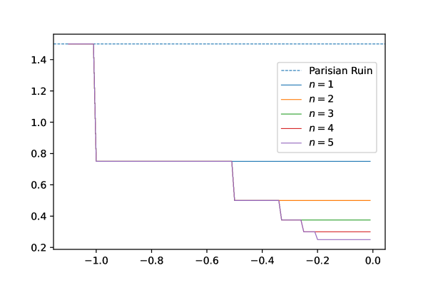
Figure 1. Bankruptcy rate functions defined in Equation (21).

In Figure 2, we plot the value functions corresponding to the bankruptcy rate functions $\omega_{n}$ defined above (in Equation (21)), with the corresponding optimal barrier levels $b_{n}^{*}$. Note that, as expected, we have that if $n_{1}<n_{2}$, then $b_{n_{2}}^{*}\leq b_{n_{1}}^{*}$. See also Figure 3.

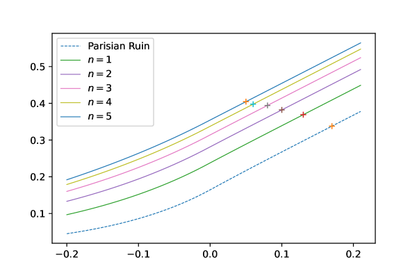
Figure 2. Value functions corresponding to the step bankruptcy rate functions defined in Equation (21), with corresponding optimal barrier levels indicated by a cross.

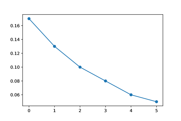
Figure 3. Optimal barrier levels corresponding to the step bankruptcy rate functions defined in Equation (21).

5.2. Affine functions

Now, we consider affine bankruptcy rate functions, i.e., of the form

$$\omega_{m}(x):=\phi\mathbf{1}_{(-\infty,a)}(x)+(\phi+m(x-a))\mathbf{1}_{[a,0)}(x),$$ (22)

for different values of $m<0$. Recall that $a=-1$ and $\phi=1.5$. Note that, if $m=0$, then $\omega_{0}=\omega_{\textsc{P}}$, i.e., it corresponds to Parisian ruin at rate $\phi$. Finally, if $m_{1}<m_{2}$, then $\omega_{m_{1}}(x)<\omega_{m_{2}}(x)$ for all $x\in(a,0)$. See Figure 4.

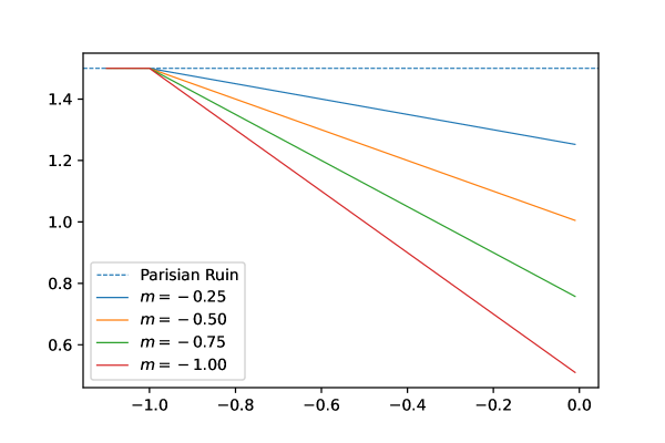
Figure 4. Bankruptcy rate functions defined in Equation (22).

In Figure 5, we plot the value functions corresponding to the bankruptcy rate functions $\omega_{m}$ defined above (in Equation (22)), with the corresponding optimal barrier levels $b_{m}^{*}$. Note that, as expected, we have that if $m_{1}<m_{2}$, then $b_{m_{2}}^{*}\leq b_{m_{1}}^{*}$. See also Figure 6.

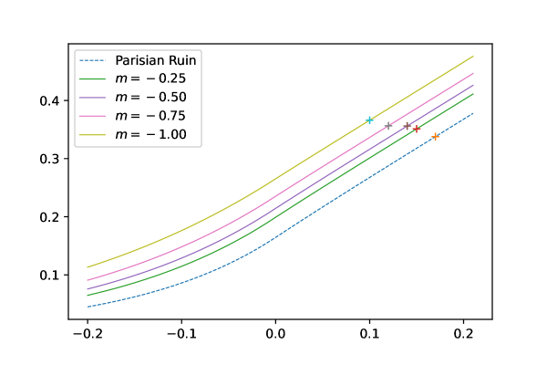
Figure 5. Value functions corresponding to the affine bankruptcy rate functions defined in Equation (22), with corresponding optimal barrier levels indicated by a cross.

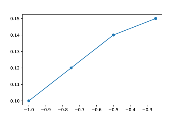
Figure 6. Optimal barrier levels corresponding to the affine bankruptcy rate functions defined in Equation (22).

Appendix A Proof of Lemma 2.1

Our proof of (4) is based on the representation of $Z_{r}(\cdot;\Phi(s))$ given in (2) and on (3). Take $x>0$ and use (2) to write

$$\int_{0}^{x}W^{(p)}(x-y)Z_{r}(y;\Phi(s))\mathrm{d}y =\int_{0}^{x}W^{(p)}(x-y)\left[(s-r)\int_{0}^{\infty}\mathrm{e}^{-\Phi(s)z}W^{(r)}(y+z)\mathrm{d}z\right]\mathrm{d}y$$

$$=(s-r)\int_{0}^{\infty}\mathrm{e}^{-\Phi(s)z}\left[\int_{0}^{x}W^{(p)}(x-y)W^{(r)}(y+z)\mathrm{d}y\right]\mathrm{d}z.$$

Using (3) to compute the inner integral and then using (2) again, we can write

$$\int_{0}^{x}W^{(p)}(x-y)Z_{r}(y;\Phi(s))\mathrm{d}y=\frac{s-r}{p-r}\left[\frac{Z_{p}(x;\Phi(s))}{s-p}-\frac{Z_{r}(x;\Phi(s))}{s-r}\right]\\ -(s-r)\int_{0}^{\infty}\mathrm{e}^{-\Phi(s)z}\left[\int_{0}^{z}W^{(p)}(x+z-y)W^{(r)}(y)\mathrm{d}y\right]\mathrm{d}z,$$

where

$$\int_{0}^{\infty}\mathrm{e}^{-\Phi(s)z} \left[\int_{0}^{z}W^{(p)}(x+z-y)W^{(r)}(y)\mathrm{d}y\right]\mathrm{d}z$$

$$=\int_{0}^{\infty}W^{(r)}(y)\left[\int_{y}^{\infty}\mathrm{e}^{-\Phi(s)z}W^{(p)}(x+z-y)\mathrm{d}z\right]\mathrm{d}y$$

$$=\frac{1}{s-p}Z_{p}(x;\Phi(s))\int_{0}^{\infty}\mathrm{e}^{-\Phi(s)y}W^{(r)}(y)\mathrm{d}y$$

$$=\frac{1}{(s-p)(s-r)}Z_{p}(x;\Phi(s)).$$

In conclusion,

$$\int_{0}^{x}W^{(p)}(x-y)Z_{r}(y;\Phi(s))\mathrm{d}y=\frac{Z_{p}(x;\Phi(s))-Z_{r}(x;\Phi(s))}{p-r}.$$

The result follows.