Interpretation of SNIa and BAO cosmic probes results using a two-regions model of the universe

1.   Introduction

One of the most intriguing mysteries of the universe is its apparent accelerated expansion. Initially, astronomers believed that the expansion of the universe, a phenomenon first observed by Edwin Hubble in the 1920s, would gradually slow down due to gravitational attraction. However, in 1998, two independent research teams ([1] and [2]) studying distant supernovae made a groundbreaking discovery: the universe is not just expanding, it is expanding at an accelerating rate. Ongoing observations, such as those involving distant supernovae, the cosmic microwave background (CMB), and large-scale structure surveys, continue to provide data, validating the first results, see for example [3], [4] (WMAP project), [5] (Planck project) and [6]. Currently, those results have led most scientists to admit that some form of energy, often referred to as "dark energy", is driving this phenomenon. However, despite being one of the most dominant components of the universe, dark energy remains one of its greatest mysteries. Several theories have been proposed to explain the nature of dark energy (such as a cosmological constant or the Quintessence theory), but none of them has been validated yet.

While the discovery of the accelerated expansion of the universe has led to the widespread acceptance of dark energy as a driving force, not all scientists agree that this interpretation is the only or even the correct explanation. Some alternative theories propose that the accelerated expansion might not be real or that our observations could be explained without invoking dark energy. Such alternative theories encompass among others modified gravity theories and inhomogeneous universe theories. In these latter ones, it is assumed that the inhomogeneities of the matter distribution lead to the accelerated expansion of the universe. Some of these theories consider this expansion as a real phenomenon, led by cosmic backreaction effects (see for example [7], [8], [9] and [10]). Other theories claim that the expansion is only an apparent phenomenon, that could originate from existing gradients in the energy associated with the varying curvature of space and the varying kinetic energy of the expansion of space ([11]), or from the fact that we perform measurements either from an underdense region ([12], [13], [14], [15], [16] and [17]), either on objects located in overdense regions only ([18]). While the idea of an accelerated expanding universe driven by dark energy remains the most widely accepted explanation, these alternative models challenge the conventional view and stimulate ongoing debate and research.

The explanation proposed by [18] considers that the apparent accelerated expansion of the universe originates from a bias in the measurements. Indeed, measurements made on SNIa or in large-scale structure surveys ar generally made on astrophysical objects located mostly in overdense regions. These overdense regions have a density larger than the average one over space, and hence are susceptible to follow a different dynamics than the one of the overall universe, supposed to obey the Friedmann equation. If it makes sense at a global scale to conceptually model the universe with the Friedmann-Lemaître-Robertson-Walker (FLRW) metric, measurements are not performed at such a scale, they are always performed on objects having micro-scale dimensions, located either in overdense regions (for most of them), either in underdense regions. If those regions do not present a metric corresponding to the FLRW one, this would mean that measurements performed on those objects are altered by the local metric. This is in particular the case for redshift measurements, largely used in cosmic probes, since frequencies depend on the local proper time. The frequency of a signal emitted from an object (or received by an observer) located in an overdense region will differ from the one emitted by the same object (or received by the same observer) if the local metric would indeed correspond to the FLRW one.

Based on this assumption, [19] developed a theoretical model to investigate on a practical point of view how SNIa measurements could be affected by this bias. This model makes the distinction between the dynamics of overdense and underdense regions, respectively, and is hence referred to as a two-regions model. It depends on one single parameter, namely the current value of the part of the volume occupied by overdense regions through space. Using a value corresponding to the one that has been estimated by several authors, it was shown that the two-regions model could explain the apparent accelerated expansion of the universe without invoking the dark energy assumption: starting from a supposed real dynamics associated to a null cosmological constant, the model predicted a measured dynamics corresponding to the observed one.

This model suffers however from some important limitations and drawbacks. The aim of this article is therefore to improve the two-regions model developed in [19], in order to (i) better highlight the link between the measured dynamics of the universe and the expected dynamics in overdense regions, and show that what we observe in practice is perhaps not the dynamics of the universe as a whole, but the dynamics of the overdense regions; (ii) apply this improved model on the Baryonic Acoustic Oscillations (BAO) as well as on the SNIa cosmic probes, to show how in practice measurements are affected by the inhomogeneities, and to highlight how from the expected classical dynamics (meaning without cosmological constant), we finally observe a dynamics with an apparent accelerated expansion.

The article is organised as follows. In Section 2 we remind the main assumption we made in the development of the original two-regions model, and the main relations that will still apply here. In Section 3, we then improve the two-regions model. Next, we apply this model on the SNIa cosmic probe (Section 4) and BAO cosmic probe (Section 5). Finally, the results are discussed in Section 6.

2.   The original two-regions model

In this Section, we remind the main results of the original two-regions model that has been developed by [19]. We limit ourselves to present the assumptions and relations that will be useful to improve this model.

As is usually done, at large scale, the two-regions model assumes that the universe can be described by the FLRW metric. This is supported by the fact that at such a scale, matter is supposed to be evenly distributed over space, meaning thus that space can be considered as homogeneous and isotropic. At a meso-scale, however, it is known that matter has grouped to form particular structures, leaving large regions of void. Since measurements are performed on astrophysical objects located mostly in overdense regions, it was suggested in [18] that it was necessary to interpret those measurements by taking into account this bias. Therefore, the two-regions model makes the distinction between underdense (void) and overdense regions, the latter ones supposed to contain all the existing matter. To do so, we follow an approach inspired from fluid mechanics for two-phase flows: in a continuum mechanics approach, we consider that both phases coexist at each point, each phase having its own properties and it own equation of state. The mixture properties correspond then to some weighted average of the properties of each phase. Similarly for the universe, if we assume that at large scale it can indeed be globally described by the FLRW metric, we also assume that each spatial point contains some part of void regions and some part of overdense regions. The specific properties (in particular the metric) of each region are such that, together, both regions lead to a global dynamics of the universe that corresponds to the one predicted by the Friedmann equation.

Admitting that the cosmological constant vanishes, the Einstein equation of General Relativity reads

$$G_{\mu\nu}=8\pi GT_{\mu\nu}\,.$$ (1)

Using this equation together with the FLRW metric, assuming a flat space, we find that the scale factor $a$ presents a dynamics verifying the Friedman equation:

$$3\frac{\dot{a}^{2}}{a^{2}}=8\pi G\rho\,,$$ (2)

where $\rho$ is the average density over space, and where $a$ has been normalized to be dimensionless, such that by convention $a=1$ at the current time. At large scale, the dynamics of the universe is thus assumed to be characterized by a global scale factor obeying Eq. $(\ref{FLRW})$. Also, since we assume that at large scale the universe can be described by the FLRW metric, it still makes sense to use the specific frame of reference based on the co-moving coordinates, for which $t$ is the cosmological time coordinate, and where $(x,y,z)$ are the spatial Cartesian coordinates.

Now, to take into account the assumption we made at a meso-scale, we consider that each point of our co-moving coordinates contain some part of underdense regions and some part of overdense regions. Let us therefore consider a volume $V$ of space sufficiently large so that it can be assumed to be representative of the universe. The average density of matter in $V$ corresponds to the density $\rho$ used in the Friedman equation. In this volume $V$, overdense regions occupy a volume $V_{o}$ and have an average density $\rho_{o}$, while underdense regions occupy a volume $V_{u}$ and have an average density $\rho_{u}$. This means that at each point on the co-moving coordinates, the part of the overdense region corresponds to $V_{o}/V$, while the part of the underdense regions corresponds to $V_{u}/V$. For simplicity, we consider in this article the limiting case for which $\rho_{u}=0$, hence underdense regions do not contain any matter.

Specific overdense and underdense regions can have extremely complicated characteristics, but we do not want to examine them in all their complexity, we only use average properties. In particular, overdense and underdense regions have their own average metric tensor. In the considered frame of reference they can be written as

$$g_{\mu\nu}=\left(\begin{array}[]{c c c c}-f_{i}^{2}&0&0&0\\ 0&b_{i}^{2}&0&0\\ 0&0&b_{i}^{2}&0\\ 0&0&0&b_{i}^{2}\end{array}\right)\,,$$ (3)

where $i=o$ for overdense regions and $i=u$ for underdense regions. Here, $f_{i}$ and $b_{i}$ are functions depending on the cosmological time $t$ at most. These functions may differ from the corresponding ones of the FLRW metric (1 and $a$ respectively), since the scale factors and the proper time in overdense and underdense regions do not necessarily evolve at the same rate.

Additionally, the stress-energy tensor of overdense regions can be written as

$$T_{\mu\nu}=\left(\begin{array}[]{c c c c}\rho_{o}f_{o}^{2}&0&0&0\\ 0&p_{o}b_{o}^{2}&0&0\\ 0&0&p_{o}b_{o}^{2}&0\\ 0&0&0&p_{o}b_{o}^{2}\end{array}\right)\,,$$ (4)

where $p_{o}$ is the average pressure in the overdense regions.

Using the metric (and its derived tensors) together with the stress-energy tensor of the overdense regions in Eq. $(\ref{GR})$, we find that

$$3\frac{\dot{b}_{o}^{2}}{b_{o}^{2}}=8\pi G\rho_{o}f_{o}^{2}\,.$$ (5)

This latter equation expresses the dynamics of the scale factor $b_{o}$ in overdense regions. A similar equation can be obtained for underdense regions, but in which the right hand side is zero, since those regions are supposed to be completely empty. This would mean that underdense regions do no expand ($\dot{b}_{u}=0$). This however does not mean that they do not grow. In fact, during the expansion of overdense regions, matter moves back towards the centre of gravity of the region, due to the gravitational attraction. In moving back, matter leaves some void that initially belonged to the overdense regions, and that hence contributes to enlarge the underdense regions. So if underdense regions do not expand by themselves, they grow by a continuous volume transfer coming from the overdense regions. This thus also means that the expansion of the universe is globally a result of the expansion of the overdense regions only. As explained in [19], in volume $V$, the expansion rate of the overdense regions corresponds to $3V_{o}\dot{b}_{o}/b_{o}$, and this quantity should be equal to the expansion rate of the whole volume $V$ at that time, being $3V\dot{a}/a$:

$$3V_{o}\frac{\dot{b}_{o}}{b_{o}}=3V\frac{\dot{a}}{a}\,.$$ (6)

Combining this latter equation with Eq. $(\ref{FLRW})$ and $(\ref{E1})$, we find that

$$f_{o}=\frac{V}{V_{o}}\sqrt{\frac{\rho}{\rho_{o}}}\,.$$ (7)

Since all existing matter is supposed to be contained in overdense regions, we have $V\rho=V_{o}\rho_{o}$. So Eq. $(\ref{fqq})$ can also be written as

$$f_{o}=\sqrt{\frac{\rho_{o}}{\rho}}=\sqrt{\frac{V}{V_{o}}}\,.$$ (8)

This quantity is larger than 1, showing that the proper time in overdense regions evolves at a rate larger than the cosmological time $t$.

Let us remind one last result of [19] that will be useful here. Cosmic probes usually involve redshift measurements. Those measurements allow to deduce the scale factor by performing a time span measure at our location. In a perfectly homogeneous and isotropic space, the scale factor can indeed be deduced by using the following relation:

$$\frac{a(t)}{a(t_{0})}=\frac{\Delta t}{\Delta t_{0}}\,,$$ (9)

where $\Delta t$ is the time span characterising some event, as measured at the point where the event occurred, and $\Delta t_{0}$ is the time span of that event as it is measured now from the earth. By convention, the scale factor at our current time $a(t_{0})$ is set at 1. Taking into account the inhomogeneities of the overdense regions on which measurements are performed, it was shown in [19] that Eq. $(\ref{pep})$ becomes

$$\frac{b_{o}(t)f_{o}(t_{0})}{b_{o}(t_{0})f_{o}(t)}=\frac{\Delta t}{\Delta t_{0}}\,.$$ (10)

When performing redshift measurements, we use Eq. $(\ref{pep})$ to determine the scale factor at some time $t$. This thus requires to measure $\Delta t/\Delta t_{0}$. In practice, however, this is not what we measure. Indeed, the time span measurement performed at our location is carried out in our proper time frame, meaning that we do not measure $\Delta t_{0}$ but instead $f_{o}(t_{0})\Delta t_{0}$. Similarly, the characteristic time span at the source is known in its proper time frame, hence it is equal to $f_{o}(t)\Delta t$ instead of $\Delta t$. So, what we measure in practice is not $\Delta t/\Delta t_{0}$, but instead

$$\frac{f_{o}(t)\Delta t}{f_{o}(t_{0})\Delta t_{0}}\,.$$ (11)

This is the measured value $a_{meas}(t)$ of the scale factor at the SNIa, given that $a(t_{0})$ is conventionally set to $1$. From Eq. $(\ref{dq})$, we deduce that

$$a_{(meas)}(t)=\frac{b_{o}(t)}{b_{o}(t_{0})}\,.$$ (12)

In general, the measured scale factor $a_{(meas)}(t)$ will differ from the real scale factor $a(t)$ at the same cosmological time $t$.

3.   The improved two-regions model

From now on, we will improve the original two-regions model, starting from the relations reminded above. Let us first highlight the need to improve this model.

Firstly, the original model considered a density in overdense regions being constant over time, assuming hence that matter has rapidly reached a state in which it is gravitationally bound. A region made of gravitationally bound matter keeps it volume constant over time, an if its matter content is also constant, its density remains indeed unchanged. This assumption puts a strong constraint on the model. Assuming that overdense regions have a constant volume makes sense as long as the overall volume of the universe is larger than the constant volume of the overdense regions. Going back in time, quite soon we reach a total volume of the universe that becomes smaller. The model is thus valid for small values of redshift only.

More importantly, since typical cosmic probes perform measurements only on objects located in overdense regions, according to the explanation proposed by [18] to understand the apparent accelerated expansion of the universe, we expect to measure a dynamics of the scale factor corresponding to the one of those regions, or at least derived from it. Let us show the limit of the original two-regions model with respect to this.

The Hubble parameter is defined as

$$H(t)=\frac{\dot{a}(t)}{a(t)}\,.$$ (13)

This is the theoretical value, meaning the one we would observe in a perfectly homogeneous space, and it verifies the Friedmann equation. In practice, however, due to the inhomogeneities, we will measure a Hubble parameter corresponding to

$$H_{(meas)}(t)=\frac{\dot{a}_{(meas)}(t)}{a_{(meas)}(t)}\,.$$ (14)

Differentiating Eq. $(\ref{jj})$ with respect to the cosmological time $t$, and including a factor $f_{o}(t)$ to take into account the fact that in practice this parameter is measured with respect to the real local time (and not the cosmological time), we get

$$H_{(meas)}(t)=\frac{1}{f_{o}(t)}\frac{\dot{b}_{o}(t)}{b_{o}(t)}\,.$$ (15)

This thus means that Eq. $(\ref{E1})$ can be written as:

$$H_{(meas)}^{2}(t)=\frac{8\pi G}{3}\rho_{o}\,.$$ (16)

This is the equivalent Friedman equation for the dynamics we measure in practice when performing redshift measurements. If $\rho_{o}$ is constant over time (as was assumed in [19] for simplicity), so will be the Hubble parameter, leading to a dynamics that does not correspond to the observed one. Assuming a constant density in overdense regions is however oversimplified, a more realistic evolution can be used. Lacking for detailed estimations of the evolution of this parameter, we we will use an approximation. This approximation can be built by taking into account the two following constraints:

• at large redshift, inhomogeneities were much smaller, tending to be negligible at the origin. So, at large redshift, the density should evolve as expected in a perfectly homogeneous and isotropic space, with a dependence in $a^{-3}$, the constant of proportionality being the average density $\rho(t_{0})$ over whole space at the current time (we neglect here the radiation era).

• the more we progress in time, the more overdense regions develop, and the more matter tends to be gravitationally bound. As explained above, when matter is gravitationally bound, its volume remains constant, and if it has a given matter content, the density is also constant. So over time, the density should tend to a constant value. This constant value corresponds to the threshold below which overdense regions cannot expand anymore, meaning that any expansion of those region will be exactly compensated by an equivalent backward motion of the matter to keep the overdense region volume constant.

Many approximations can be proposed in this way. For example, the following relation verifies those two constraints:

$$\rho_{o}=\rho_{\Lambda}+\rho(t_{0})b_{o}^{-3}(t)\,,$$ (17)

where $\rho_{\Lambda}$ is a constant corresponding to the threshold mentioned above. For the second term of the right hand side, a dependence on the scale factor of the overdense regions has been preferred than on the scale factor $a$, since the density is defined with respect to the local volume, being proportional to $b_{o}^{3}(t)$. At large redshift, the first term of the right hand side will become negligible with respect to the second term, and since $b_{0}(t)$ is expected to tend to the scale factor of the universe $a$ at those times (due to negligible inhomogeneities), $\rho_{o}$ will indeed present the expected trend, being $\rho(t_{0})a^{-3}$. On the other hand, at larger times, the second term of the right hand side will become negligible with respect to the first term, and $\rho_{o}$ will tend to a constant value.

We stress that $\rho(t_{0})$ is the average density over whole space, and this quantity is thus usually expressed with respect to the FLRW metric. On the other hand, in Eq. $(\ref{Hm})$, we have expressed the Hubble parameter with respect to our local frame (given the metric of overdense regions), by using the factor $f_{o}(t_{0})$ to take into account that the local time unit differs from the one in the FLRW metric. To remain consistent, we do the same for the density, and we multiply $\rho(t_{0})$ by $b_{o}^{3}(t_{0})$ to convert spatial dimensions from the FLRW metric to the ones of our local metric. Hence, Eq. $(\ref{uy})$ becomes

$$\rho_{o}=\rho_{\Lambda}+\rho_{(meas)}(t_{0})\frac{b_{o}^{3}(t_{0})}{b_{o}^{3}(t)}\,,$$ (18)

where $\rho_{(meas)}(t_{0})$ is the current average density, expressed in our local frame.

Let us also stress that Eq. $(\ref{uy2})$ is one approximation amongst many others that verify the two mentioned constraints. More complex approximations could be build to allow for an evolving cosmological constant for example. The approximation of Eq. $(\ref{uy2})$ has been selected because it is the one that will highlight the best the effect of the inhomogeneities on the as observed evolution of the expansion of the universe, by distinguishing two terms, one related to the expected behaviour, and one related to an apparent cosmological constant. Indeed, let us first notice that, given Eq. $(\ref{jj})$, Eq. $(\ref{uy2})$ can also be written as

$$\rho_{o}=\rho_{\Lambda}+\rho_{(meas)}(t_{0})a_{(meas)}^{-3}\,.$$ (19)

Then, including this latter equation into Eq. $(\ref{Hm})$, we obtain

$$H_{(meas)}^{2}=\frac{8\pi G}{3}\left(\rho_{\Lambda}+\rho_{(meas)}(t_{0})a_{(meas)}^{-3}\right)\,.$$ (20)

Interestingly, Eq. $(\ref{fqqx})$ describes a dynamics equivalent to what we observe in practice, suggesting the fact that perhaps we do not measure the dynamics of the universe as a whole, but the dynamics of the overdense regions only.

If at the early times the observed behaviour corresponds to what we expect, it is because inhomogeneities were relatively small: overdense regions did almost span the whole universe, and both dynamics were quite similar. Then, over time, overdense regions have developed, and their average density tends to some threshold at which all matter has reached a gravitationally bound state. This threshold density $\rho_{\Lambda}$ behaves exactly as a cosmological constant in the dynamics of the overdense regions. Let us also notice that applying the conservation law $\nabla_{\mu}T^{\mu}_{\ 0}=0$ to the stress-energy tensor of the overdense regions, we get

$$\dot{\rho_{o}}=-3\frac{\dot{b}}{b}\left(\rho_{o}+p_{o}\right)\,.$$ (21)

When the density of the overdense regions has reached its threshold, we have $\dot{\rho_{o}}=0$, meaning that $p_{o}=-\rho_{o}$, explaining here also why, at that time, matter in overdense regions will behave as dark energy. The negative pressure of matter in overdense regions is related to the backward motion of the matter during the expansion of overdense regions, due to the gravitational attraction.

Let us now establish the evolution of the scale factor $b_{o}(t)$ in overdense regions. Instead of determining its evolution in function of the cosmological time $t$, we will determine it in function of the scale factor $a$. We therefore start from Eq. $(\ref{fq})$, which can be written as

$$\frac{db_{o}}{da}=\frac{V}{V_{o}}\frac{b_{o}}{a}=\frac{\rho_{o}}{\rho}\frac{b_{o}}{a}\,.$$ (22)

Using Eq. $(\ref{uy})$ to express $\rho_{o}$ in function of $b_{o}$, and using also $\rho=\rho(t_{0})a^{-3}$, we get

$$\frac{db_{o}}{da}=\frac{\rho_{\Lambda}+\rho(t_{0})b_{o}^{-3}}{\rho(t_{0})}b_{o}a^{2}\,.$$ (23)

This differential equation has one single physical solution:

$$b_{o}(t)=\sqrt[3]{\frac{\exp{\left(\frac{\rho_{\Lambda}}{\rho(t_{0})}a^{3}+c_{1}\rho_{\Lambda}\right)}-\rho(t_{0})}{\rho_{\Lambda}}}\,,$$ (24)

where $c_{1}$ is a constant to determine. We constrain $b_{o}$ to tend to $0$ when $a$ tends to $0$. This implies that $\exp{\left(c_{1}\rho_{\Lambda}\right)}=\rho(t_{0})$, and we finally obtain:

$$b_{o}(t)=\sqrt[3]{\frac{\rho(t_{0})}{\rho_{\Lambda}}\left[\exp{\left(\frac{\rho_{\Lambda}}{\rho(t_{0})}a^{3}\right)}-1\right]}\,.$$ (25)

Together, Eq. $(\ref{a1})$ for $f_{o}$ and Eq. $(\ref{da})$ for $b_{o}$ completely determine the evolution of the metric of the overdense regions over time.

4.   Application of the two-regions model to the SNIa cosmic probe

In this section we see how measurements performed in the frame of the SNIa cosmic probe are affected by the inhomogeneities, and how this can lead to the apparent dynamics we observe in practice. To explain why this cosmic probe lead to the observation of an accelerated expansion of the universe, we will show that all kinds of measurements performed for this cosmic probe can in some way be related to the apparent scale factor $a_{(meas)}$, which verifies the dynamics expressed by Eq. $(\ref{fqqx})$. More exactly, we will show that all measured quantities verify a dynamics expressed by the usual corresponding laws, in which however the scale factor $a$ has been replaced by the apparent scale factor $a_{(meas)}$.

Two kinds of measurements are performed for the SNIa cosmic probe: redshift measurements, and luminosity distance measurements. We have already reminded how redshift measurement are affected, see Eq. $(\ref{jj})$, showing that such measurements indeed lead to observe the apparent scale factor $a_{(meas)}$ instead of the real scale factor $a$.

We thus now investigate the effect on luminosity distance measurements. The luminosity distance $d_{L}$ is defined as

$$d_{L}^{2}=\frac{L}{4\pi F}\,,$$ (26)

where $L$ is the absolute luminosity emitted at the source of the SNIa, and $F$ is the flux measured at our location. When applying this relation, $L$ is supposed to be known, and we measure $F$, from which we then deduce $d_{L}$.

For practical reasons, we will slightly adapt the definition of the luminosity distance $d_{L}$. We define

$$d_{L}^{2}=\frac{L(\Omega)}{\Omega F}\,,$$ (27)

where $L(\Omega)$ is the part of the absolute luminosity (supposed to be isotropic) emitted in the solid angle $\Omega$. Quantitatively, this definition is equivalent to the original one, and obviously, the original definition corresponds to $\Omega=4\pi$. The reason for which we adapt the usual definition is that in practice flux measurements are never performed along the whole solid angle, but only on a small portion of it. This has no consequences in the case of the perfect homogeneous space, but the new definition will be more practical in the case of the heterogeneous space.

Let us first consider the case of a perfect homogeneous space. The energy emitted by the source will by diluted first because photons are spread over an increasing surface, but also by two additional effects: (i) photons redshift by a factor $z$, and (ii) photons hit the surface at the observer’s location less frequently, since two photons separated initially by a time $\Delta t$ will be measured at a time $(1+z)\Delta t$ apart. Hence

$$\frac{F}{L(\Omega)}=\frac{1}{(1+z)^{2}A}=\frac{a^{2}}{A}\,,$$ (28)

where $A$ is the surface on which the observer performs the flux measurement. It corresponds to the part generated by the solid angle $\Omega$ on the sphere centred at the source (supposed to be located at comoving distance $X$ from us), and whose radius corresponds to the distance travelled by light from the source up to the earth:

$$A=\Omega\left(a(t_{0})X\right)^{2}\,.$$ (29)

For a null geodesic we have

$$0=-dt^{2}+a^{2}dx^{2}\,,$$ (30)

so

$$X=\int_{0}^{X}dx=\int_{t_{0}}^{t}\frac{dt}{a}=\int_{a(t_{0})}^{a(t)}\frac{da}{a^{2}H(a)}\,,$$ (31)

and

$$A=\Omega\left(\int_{a(t_{0})}^{a(t)}\frac{da}{a^{2}H(a)}\right)^{2}\,.$$ (32)

Knowing the surface $A$ and the scale factor $a$ at the source, we can determine the luminosity distance $d_{L}$.

Before investigating the case of the heterogeneous space, it will be useful to provide a different physical interpretation to Eq. $(\ref{surf})$. The surface $A$ has been calculated from the comoving distance $X$ separating the observer and the source. This surface is perpendicular to the line of sight, and can thus also be expressed in terms of the other coordinates. If the solid angle $\Omega$ is small, the surface $A$ is almost planar, and we can for simplicity consider a rectangular surface that can be expressed as $a(t_{0})^{2}\Delta Y\Delta Z$, where $\Delta Y$ and $\Delta Z$ are the comoving dimensions of the surface along the $y$ and $z$ coordinates, respectively. We need now to determine those quantities.

The surface $A$ is delimited by the most outward photons of the flux sent by the source and that will hit that surface at the observer’s location. We thus focus on these photons. Let $\theta_{y}$ be the angle made between the upper and lower light beam in the $x-y$ plane to span, from the source, the segment of length $\Delta Y$ located at the earth’s position. Similarly, let $\theta_{z}$ be the equivalent angle in the $x-z$ plane to span, from the source, the segment of length $\Delta Z$. Together, $\theta_{y}$ and $\theta_{z}$ constitute the solid angle $\Omega$.

During the propagation of the light beams, when photons travel a distance $dt$, the comoving coordinate of the height of the surface $A$ at the observer’s location grows by a quantity $dy$ such that

$$a(t)dy=\theta_{y}dt\,,$$ (33)

meaning thus that

$$dy=\frac{\theta_{y}}{a(t)}dt\,.$$ (34)

To determine $\Delta Y$, we have to integrate this last relation along the trajectory of the photons, from the source up to the observer:

$$\Delta Y=\int dy=\theta_{y}\int\frac{dt}{a(t)}\,.$$ (35)

From Eq. $(\ref{gg})$, we can convert $dt$ into $da$:

$$dt=\frac{da}{a(t)H(t)}\,,$$ (36)

so Eq. $(\ref{qp})$ can be written as

$$\Delta Y=\theta_{y}\int\frac{da}{a^{2}(t)H(t)}\,.$$ (37)

Multiplying with the equivalent result for $\Delta Z$, we get the same relation for $A$ as expressed in Eq. $(\ref{surf})$. The advantage of the approach we followed is that it provides a useful physical interpretation of the integral in this latter relation.

We now apply the same approach in the case of the heterogeneous space, for which the surface that will be hit by the photons lies in an overdense region, expanding at a different rate than the global universe. This means that while the outward photons travel a distance $dt$, the comoving coordinate of the height of the surface $A$ at the observer’s location increases of a quantity $dy$ such that

$$b_{o}(t)dy=\theta_{y}dt\,,$$ (38)

where we now used the local scale factor $b_{o}(t)$ of the overdense regions. So

$$\Delta Y=\int dy=\theta_{y}\int\frac{dt}{b_{o}(t)}\,.$$ (39)

Using now the fact that

$$H_{meas}(t)=\frac{\dot{b}_{o}(t)}{b_{o}(t)}\,,$$ (40)

we may write Eq. $(\ref{qp1})$ as

$$\Delta Y=\theta_{y}\int\frac{db_{o}}{b_{o}^{2}(t)H_{meas}(t)}\,.$$ (41)

Using the equivalent relation for $\Delta Z$, we find that

$$A=\Omega\left(\int_{b_{o}(t_{0})}^{b_{o}(t)}\frac{db_{o}}{b_{o}^{2}(t)H_{(meas)}(t)}\right)^{2}\,.$$ (42)

Let us now go back to Eq. $(\ref{Fl})$ and see what this relation becomes in the case of the heterogeneous space. On the left hand side, the flux is measured in the referential of the observer, meaning that distances and times are defined with respect to the local metric, which differs from the FLRW metric. The flux is expressed per unit surface and per unit time, therefore we need to take into account a correction factor $b_{o}^{2}(t_{0})$ for the surface and a correction factor $f_{o}(t_{0})$ for the time. Similarly, the absolute luminosity of the source is defined with respect to its proper time, so here we need to take into account a correction factor $f_{o}(t)$.

On the right hand side, firstly, the redshift that has occurred due to the spatial expansion now corresponds to a dilution factor $b_{o}(t_{0})/b_{o}(t)$. Secondly, as shown by Eq. $(\ref{dq})$, in the cosmological time frame, the ratio between the time span at the source and the one measured by the observer is $b_{o}(t_{0})f_{o}(t)/b_{o}(t)f_{o}(t_{0})$. Thirdly, the surface $A$ is now modified according to Eq. $(\ref{Su})$.

In summary, we have:

$$\frac{Fb_{o}^{2}(t_{0})f_{o}(t_{0})}{L(\Omega)f_{o}(t)}=\frac{b_{o}(t)}{b_{o}(t_{0})}\frac{b_{o}(t)f_{o}(t_{0})}{b_{o}(t_{0})f_{o}(t)}\left[\Omega\left(\int_{b_{o}(t_{0})}^{b_{o}(t)}\frac{db_{o}}{b_{o}^{2}(t)H_{(meas)}(t)}\right)^{2}\right]^{-1}\,.$$ (43)

Simplifying this relation, we get

$$\frac{F}{L(\Omega)} = \frac{b_{o}^{2}(t)}{b_{o}^{2}(t_{0})}\left[\Omega\left(\int_{b_{o}(t_{0})}^{b_{o}(t)}\frac{b_{o}^{2}(t_{0})}{b_{o}^{2}(t)H_{(meas)}(t)}\frac{db_{o}}{b_{o}(t_{0})}\right)^{2}\right]^{-1}$$ (44)

$$= a_{(meas)}^{2}\left[\Omega\left(\int_{a_{(meas)}(t_{0})}^{a_{(meas)}(t)}\frac{da_{(meas)}}{a_{(meas)}^{2}(t)H_{(meas)}(t)}\right)^{2}\right]^{-1}\,,$$

where we used the fact that $b_{o}(t)/b_{o}(t_{0})=a_{(meas)}$. This means that Eq. $(\ref{Fl})$ remains applicable to determine the flux that will be measured at the observer’s location, except that all parameters involving the scale factor $a$ are modified in such a way that they now involve the apparent scale factor $a_{(meas)}$. As a consequence, the luminosity distance as determined from Eq. $(\ref{qw})$ will exhibit a dynamics corresponding to the one followed by $a_{(meas)}$, showing hence an apparent accelerating expansion.

5.   Application of the two-regions model to the BAO cosmic probe

In this Section we will see how results obtained with the BAO cosmic probe are affected by the inhomogeneities in the overdense regions. Using the BAO cosmic probe requires performing a three-dimensional survey of the positions of specific astrophysical objects to establish a correlation function of the matter distribution. From this information, at a given redshift, the BAO peak can first be determined along the line of sight, from which we deduce the expansion rate of the universe (or Hubble parameter):

$$H(z)=\frac{c\Delta z}{r_{s}}\,,$$ (45)

where $\Delta z$ is the redshift separation corresponding to the BAO peak, and $r_{s}$ is the sound horizon at decoupling.

Secondly, the BAO peak can also be determined perpendicular to the line of sight, corresponding to an angle $\Delta\theta$, from which we deduce the angular-diameter distance $D_{A}$:

$$D_{A}(z)=\frac{r_{s}}{(1+z)\Delta\theta}\,.$$ (46)

It has to be noted that the angular-diameter distance can be related to the Hubble parameter through the following relation:

$$D_{A}(z)=\frac{1}{1+z}\int_{0}^{z}\frac{c}{H(z^{\prime})}dz^{\prime}\,.$$ (47)

Since the astrophysical objects on which we perform the three-dimensional survey are mostly located in overdense regions, this cosmic probe will be affected by the inhomogeneities of those regions, and, as a consequence, an apparent dynamics different from the expected one could be observed. We will in particular investigate how the inhomogeneities affect the equations $(\ref{x1})$ and $(\ref{x2})$ which are used for this cosmic probe.

Let us first examine the influence of the local metric on the measure of the Hubble parameter. In Eq. $(\ref{x1})$, $c$ and $r_{s}$ are constant values and do not depend on the way measurements are performed. However, $\Delta z$ will depend on the local metric, meaning that the as measured value will differ from the real value. This quantity can be written as

$$\Delta z=\Delta\left(\frac{1}{a}\right)\,.$$ (48)

We may approximate the scale factor at the points between which $\Delta z$ is measured as

$$a_{i}=a\pm\frac{\Delta a}{2}\,,$$ (49)

where $i$ stands for making the distinction between the two points, and where $a$ is the scale factor at a redshift $z$. Neglecting then second order terms, we show that

$$\Delta z=\frac{\Delta a}{a^{2}}\,.$$ (50)

So, comparing the real and the measured values of the Hubble parameter, respectively $H(t)$ and $H_{(meas)}(t)$, we have from Eq. $(\ref{x1})$

$$\frac{H_{(meas)}}{H}=\frac{\Delta a_{(meas)}}{\Delta a}\frac{a^{2}}{a^{2}_{(meas)}}\,.$$ (51)

Since the points between which $\Delta z$ is determined are in the close neighbourhood of the point at redshift $z$ where we perform the BAO measurement (meaning that $z$ and thus $a$ will not vary significantly over this distance), we may use a first order approximation, and consider that the two points for which $\Delta a$ is determined can be estimated as

$$a(t\pm\frac{\Delta t}{2})=a(t)\pm\dot{a}\frac{\Delta t}{2}\,,$$ (52)

where $\Delta t$ is the time span between the two points. In a perfectly homogeneous space, this time span is the one for light to travel the distance between these two points:

$$\Delta t=\frac{r_{s}a}{c}\,.$$ (53)

For the measured scale factor $a_{(meas)}$, on the other hand, we need to be cautious, because the measured time span between the two points will be different. However, this time is also characterized in such a way that the time span between the two points is the one for light to travel the distance (now measured with an apparent scale factor $a_{(meas)}$) between them:

$$\Delta t_{(meas)}=\frac{r_{s}a_{(meas)}}{c}\,.$$ (54)

From Eq. $(\ref{za2})$ and $(\ref{za})$, we notice that $\Delta t/a=\Delta t_{(meas)}/a_{(meas)}$ is constant, and this result will be used a little bit further.

Combining now all last relations, we find

$$\frac{H_{(meas)}(t)}{H(t)} = \frac{\dot{a}_{(meas)}\Delta t_{(meas)}}{\dot{a}\Delta t}\frac{a^{2}}{a^{2}_{(meas)}}$$ (55)

$$= \frac{\dot{a}_{(meas)}}{a_{(meas)}}\frac{a}{\dot{a}}\frac{\Delta t_{(meas)}}{a_{(meas)}}\frac{a}{\Delta t}$$

$$= \frac{\dot{b}_{o}(t)/b_{o}(t_{0})}{b_{o}(t_{0})/b_{o}(t)}\frac{1}{H(t)}\,,$$

hence

$$H_{(meas)}(t)=\frac{\dot{b}_{o}(t)}{b_{o}(t)}\,.$$ (56)

Finally, taking into account the fact that the Hubble parameter is measured from our location, which has a different proper time than the cosmological time, we get the same result as the one obtained above (Eq. $(\ref{Hub})$), where we started directly from the definition of the Hubble parameter. So, applying Eq. $(\ref{x1})$ will lead to an apparent dynamics of the scale factor in agreement with the one predicted by Eq. $(\ref{fqqx})$.

We now investigate how the inhomogeneity of space can affect the determination of the angular-diameter distance $D_{A}$ using Eq. $(\ref{x2})$. In this relation, $r_{s}$ is not affected by the inhomogeneity. We could a priori think that $\Delta\theta$ is not affected neither, because the inhomogeneities should not deviate the direction of the light beams. However, it is important to stress that we do not directly measure an angle between two points, $\Delta\theta$ is on the contrary determined after having mapped the astrophysical objects through space in the frame of the large survey. This mapping is performed by converting redshift values into distances by assuming a redshift-distance relation, based initially on a fiducial model. The correctness of this assumed relation is verified at the end of the process, and the relation is modified if necessary, up to when a good agreement is obtained between assumed and observed redshift-distance relations.

Now, the whole process depends on how the mapping is performed, and this one mainly depends on the redshift measurements. Obviously, the mapping based on the as measured redshift will differ from the mapping based on the real redshift. Combining Eq. $(\ref{x2})$ and $(\ref{x3})$, we can determine how the angle $\Delta\theta$ will depend on the redshift, and hence on the mapping:

$$\Delta\theta(z)=r_{s}\left(\int_{0}^{z}\frac{c}{H(z^{\prime})}dz\right)\,.$$ (57)

In this relation, the mapping process completely determines the right hand side. If the mapping is performed with an apparent redshift evolution that follows the dynamics described by $(\ref{fqqx})$, involving a cosmological constant, anything that will be deduced from this mapping (in particular $\Delta\theta$) will necessarily evolve according to this dynamics. Therefore, the angular-diameter distance $D_{A}$ we deduce from the measure of the angle will correspond to the one of a universe with a cosmological constant.

6.   Discussion

According to the proposed explanation, the metric presents over space a profile that is far from being perfectly homogeneous. Variations exist between overdense and underdense regions, which are sufficiently significant to lead to different dynamics between these regions and the universe considered as a whole. To evaluate the significance of these variations, it would be interesting to quantify some parameters that have been considered in the two-regions model. To fix ideas (the exact values of some parameters are still a matter of debate), we consider as an order of magnitude a measured Hubble constant of $H_{0(meas)}=70\,(km/s)/Mpc$. We also admit that the density parameter for the apparent cosmological constant is currently equal to $\Omega_{\Lambda 0}=0.7$, whereas the density parameter for the apparent matter density is currently equal to $\Omega_{M0}=0.3$.

From the apparent dynamics we measure in practice, as expressed by Eq. $(\ref{fqqx})$, we deduce

$$\rho_{\Lambda} = \frac{3}{8\pi G}\Omega_{\Lambda 0}H^{2}_{0(meas)}=6.44\times 10^{-27}\,kg/m^{3}\,,$$ (58)

$$\rho_{(meas)}(t_{0}) = \frac{3}{8\pi G}\Omega_{M0}H^{2}_{0(meas)}=2.76\times 10^{-27}\,kg/m^{3}\,.$$ (59)

Reminding that $\rho(t_{0})=\rho_{(meas)}(t_{0})b_{o}^{3}(t_{0})$, we deduce from Eq. $(\ref{da})$:

$$\rho_{(meas)}(t_{0})=\frac{\rho(t_{0})}{b_{o}^{3}(t_{0})}=\frac{\rho_{\Lambda}}{\exp{\left(\frac{\rho_{\Lambda}}{\rho(t_{0})}\right)-1}}\,,$$ (60)

from which we determine

$$\rho(t_{0})=\frac{\rho_{\Lambda}}{\ln{\left(\frac{\rho_{\Lambda}}{\rho_{(meas)}(t_{0})}+1\right)}}=5.36\times 10^{-27}\,kg/m^{3}\,.$$ (61)

Since space is assumed to be globally flat, from $\rho(t_{0})$ we may deduce the Hubble constant as it would be measured in a perfectly homogeneous space:

$$H_{0}=\sqrt{\frac{3\pi G}{8}\rho(t_{0})}=53\,(km/s)/Mpc\,.$$ (62)

Obviously, this value differs from the different estimations that have been provided for this parameter, using various techniques (see for example [20]). All these techniques however rely on measurements performed on astrophysical objects, which are mostly located in overdense regions, and which present hence the same bias as the one investigated here.

Given these values, we can establish how the scale factor $b_{o}$ in overdense regions evolves over time and compare it with the scale factor $a$ of the universe. The result is presented in Figure 1. As expected, at large redshift, $b_{o}$ converges towards $a$, but at small redshift, it significantly deviates from it. Currently, overdense regions have expanded in such a way that the local scale factor is about 1.25 times larger than the scale factor of the universe.

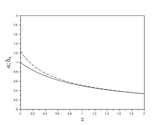
Figure 1: Evolution of $a$ (solid line) and $b_{o}$ (dashed line) in function of $z$.

In Figure 2 we present the evolution of $f_{o}$ in function of the redshift. This illustrates how proper time in overdense regions evolves with respect to the one of the universe. Here also, at large redshift, where inhomogeneities were small, $f_{o}$ tends to $1$, as expected, but at small redshift, it deviates from this value. Currently, the rate at which proper time evolves in overdense regions is about 1.3 times larger than in the FLRW metric.

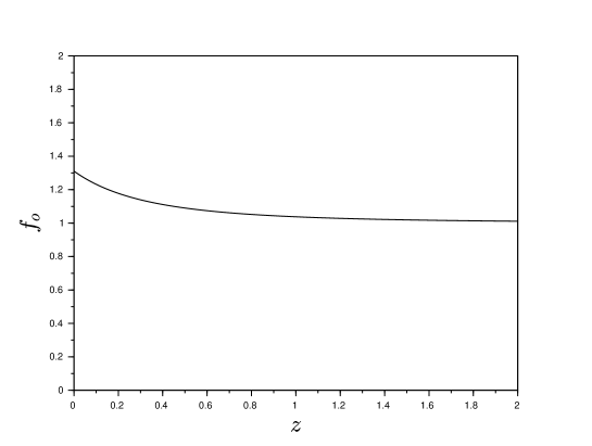
Figure 2: Evolution of $f_{o}$ in function of $z$.

It is also interesting to notice that, on the basis of the theory we have developed, we may provide on explanation of the tension highlighted between SNIa and BAO probes on the one hand and the Cosmic Microwave Background (CMB) probe on the other hand. These three cosmic probes lead to similar results, all evidencing an apparent acceleration of the expansion of the universe. Though, the results obtained with the CMB probe present with respect to the results obtained with the two other probes some slight differences, see [21].

In performing measurements to determine the evolution of the scale factor, we carry out a fitting process. The universe may present a quite complex geometrical structure, for practical purposes we assume it can globally be characterized by the FLRW metric containing a single time depending parameter, so the aim of the measurements is to fit as best as we can this FLRW metric on the real one. How this fitting is performed obviously may depend on the cosmic probe that is used. To understand the intriguing situation of the tension problem, it is important to have a clear view on the fitting processes related to each cosmic probe. We keep also in mind that, at least according to the proposed explanation in this article, space is not perfectly homogeneous. The metric may present over space significant variations. In this article, for simplicity, we have considered two regions, each one being characterized by a homogeneous metric. But in reality, we should expect some variations inside those subregions as well. All overdense regions will most probably not present exactly the same perturbation with respect to the FLRW metric.

The SNIa and BAO cosmic probes correspond to fitting processes that are conceptually identical: measurements are performed on large samples of events, covering different epochs and regions of the universe (although being part of the overdense regions). Each specific result will be affected by the local perturbation that exists with respect the FLRW metric, but in the fitting process, all results will be averaged over thanks to the size of the sample being used. At the end, the resulting evolution can hence be considered as a mean behaviour. As shown above, we measure hence with these two cosmic probes the average dynamics of the overdense regions.

On the other hand, the CMB cosmic probe presents a completely different fitting process. Let us first briefly remind the principle of this probe. The cosmic microwave background, which fills all space, is the remnant electromagnetic radiation from an early stage of the universe. This cosmic microwave background, although being almost isotropic, presents slight anisotropies. When analysing these anisotropies in terms of their power spectrum, specific peaks appear. Such peaks are the signatures of some physical phenomena, which can be related to different parameters of interest, in particular the curvature of the universe, the baryon density, and the dark-matter density. After having determined these parameters from the CMB anisotropies, the dark energy density can be deduced.

We first notice that the CMB probe is an indirect probe for the dynamics of the universe. It does not directly measure the scale factor as does the SNIa probe, but on the contrary determines the overall dynamics indirectly on the basis of other types of measurements. Conceptually, this is not an issue. If the physics is well-understood and well-described, the equations of the model predicting the CMB anisotropies should form a coherent set, and the knowledge of some parameters should allow us to determine some other ones.

Secondly, unlike the SNIa and BAO probes, the CMB probe does not track the scale factor at different times. This is a disadvantage. Indeed, this means that we have no information allowing to confirm (or not) that the temporal evolution of the scale factor indeed corresponds to the one predicted by the Friedmann equation. On the contrary, the CMB probe postulates that this temporal evolution will correspond to the one predicted by the Friedmann equation. As a consequence, the idealized manifold that we fit on the real universe is constrained by this postulate: it corresponds to a well-defined function, parametrized by the cosmological constant $\Lambda$, whose value is deduced from the measurements of curvature as well as the baryon and dark matter densities. Conceptually, this could be an issue, but on a practical point of view, the similar results obtained by the SNIa and BAO probes may support this approach.

At last, the CMB probe as it is (and can practically be) applied suffers from a major drawback. Contrary to the SNIa and BAO probes, the CMB probe provides only one single measurement that can be used to fit the FLRW metric. This single measurement depends on how the anisotropies are observed from our particular location. These measurements necessarily are affected by the perturbations of the metric existing at the locations were they have been carried out, i.e., in the vicinity of the earth. The earth is located in an overdense region, and as such we should expect that the result obtained by the CMB probe should be affected as for the SNIa and BAO probe. However, if in the simplified model we developed above we assumed homogeneous overdense regions, in reality perturbations may exist in those regions. This means that the metric at the earth location most probably does not exactly correspond to the average one characterizing the overdense regions. And since we have only one single result to fit the FLRW metric, perturbations are not averaged over, so we constrain the FLRW metric to correspond to the one existing at the earth’s location. In other words, according to this theory, the tension problem should be related to the difference existing between the average metric in overdense regions, and the real metric in the vicinity of the earth. Obviously, this is not a demonstration and further investigation is needed to confirm (or not) this explanation. This is however beyond the scope of this article.

Let us finally discuss how the two-regions model could be validated. Unfortunately, all kinds of measurements involve a source of information and an observer, and generally, at least one of them lies in an overdense region, which may hence affect the result of the measurement. However, if we could perform measurements on objects located in underdense regions, we may expect to observe a different dynamics than the one observed in overdense regions. Contrary to what has been assumed in the model, underdense regions are not completely empty, and are thus able to send some information also. SNIa are probably infrequent in these regions, and the BAO and CMB cosmic probes are not suited for this, therefore new methods should be developed. Perhaps a comparative method could be used. For example, if in some way we know that an underdense regions lies in the close neighbourhood of an overdense regions, comparing their respective redshift would allow to verify if they are similar (as predicted by the usual approach) or different (as predicted by the two-regions model). This certainly requires further research.

7.   Conclusion

Measurements performed to probe the universe use information that has been sent by astrophysical objects which are mostly located in overdense regions, where matter has grouped together. This means that such measurements could present a bias, since underdense (void) regions do not contribute to the determination of the dynamics of the universe. This would not be an issue if both regions can be considered, separately, as being representative of the universe as a whole. However, since according to the Einstein equation of General Relativity, the dynamics is a function of the local density, different dynamics could be expected between both kinds of region. Considering also that the dynamics that is observed corresponds to a total density that evolves according to a trend that resembles the one that could be expected for the density in overdense regions, the aim of the article was to investigate if this could be more than a simple coincidence. More particularly, a model has been developed to verify if the apparent accelerated expansion of the universe could be explained by the fact that we measure the dynamics of the overdense regions only, instead of the one of the global universe.

The model that has been developed corresponds to an improvement of the two-regions model developed by [19]. This model takes into account the existence of two distinct regions, namely overdense and underdense regions, each one having its own average metric. The metrics of these regions are such that, together, they lead to a global behaviour corresponding to what is expected from the Friedmann equation, assuming a null cosmological constant. The model has then been applied to the SNIa and BAO cosmic probes, with the aim to understand how in practice the inhomogeneities affect the measurements of the different parameters. Using the two-regions model, it has been shown that all these parameters depend on the redshift according to the usual theoretical relations, except that in these relations, all quantities that are related to the redshift do now depend on a measured redshift, whose dynamics involves an apparent cosmological constant. This result clearly suggests that the apparent accelerated expansion of the universe could be an artefact explained by the bias in the measurements, related to the existence of distinct regions in the universe.

Moreover, the proposed explanation provides an explanation for the tension observed between SNIa and BAO results, on the one hand, and CMB results on the other hand. The explanation is related to the fact that the first cosmic probes perform measurements on a large samples of events, covering different epochs and regions of the universe (being part of overdense regions however). Each specific measurement is affected by the local perturbation existing with respect to the FLRW metric, but in the end they are averaged over to provide a mean dynamics of overdense regions. On the other hand, the CMB cosmic probe provides only one single measurement, the one that can be performed from our particular location. The result of this measure is also affected by the local perturbation, but it is highly improbable that this perturbation corresponds to the average one that would characterize all overdense regions. The local metric being slightly different, the dynamics being deduced leads inevitably to a slightly different behaviour. This explanation needs certainly further confirmation.

References

- [1] Ries A. G. et al. [Supernova Search Team Collaboration], 1998, Observational evidence from supernovae for an accelerating universe and a cosmological constant, Astron. J., Vol. 116, Issue 3, pp. 1009-1038
- [2] Perlmutter S. et al. [Supernova Cosmology Project Collaboration], 1999, Measurements of Omega and Lambda from 42 High Redshift Supernovae, Astrophys. J., Vol. 517, pp. 565-586
- [3] D. M. Scolnic et al., 2018 The Complete Light-curve Sample of Spectroscopically Confirmed SNe Ia from Pan-STARRS1 and Cosmological Constraints from the Combined Pantheon Sample, Astrophys. J., Vol. 859, 101
- [4] C. L. Bennet et al., 2013 Nine-year Wilkinson Microwave Anisotropy Probe (WMAP) observations: final maps and results, Astrophys. J. Sup. Series, Vol. 208, 20
- [5] N. Aghanim et al. (Planck Collaboration), 2020 Planck 2018 results. VI. Cosmological parameters, Astron. Astrophys., Vol. 641, A6
- [6] D. J. Eisenstein et al., 2005 Detection of the Baryon Acoustic Peak in the Large-Scale Correlation Function of SDSS Luminous Red Galaxies Astrophys. J., Vol. 633, pp. 560
- [7] T. Buchert, 2008, Dark Energy from structure: a status report Gen. Rel. Grav., Vol. 40, pp. 467
- [8] E. W. Kolb, 2011, Backreaction of inhomogeneities can mimic dark energy Class. Quantum Grav., Vol. 28, 164009
- [9] T. Clifton, 2013, Back-reaction in relativistic cosmology Int. J. Mod. Phys., D 22, 1330004
- [10] T. Buchert et al., 2015, Is there proof that backreaction of inhomogeneities is irrelevant in cosmology? Class. Quantum Grav., Vol. 32, 215021
- [11] D. L. Wiltshire, 2007, Cosmic clocks, cosmic variance and cosmic averages New J. Phys., Vol. 9, 377
- [12] Do we really see a cosmological constant in the supernovae data? M.-N. Célérier, Astron. Astrophys. D 353 (2000)
- [13] Is dark energy the only solution to the apparent acceleration of the present universe? H. Iguchi, T. Nakamura and K. Nakao, Prog. Theor. Phys. 108 (2002) 809
- [14] Inhomogeneous alternative to dark energy? H. Alnes, M. Amarzguioui, O. Gron, Phys. Rev. D, 73 (2006) 083519
- [15] Establishing homogeneity of the universe in the shadow of dark energy M. Ishak, J. Richardson, D. Whittington and D. Garred, Phys. Rev. D 78 (2008) 123531
- [16] Local void vs dark energy: confrontation with WMAP and type Ia supernovae S. Alexander, T. Biswas, A. Notari and D. Vaid, J. Cosmol. Astropart. Phys. Vol 9 (2009) 025
- [17] Constraints on large-scale inhomogeneities from WMAP5 and SDSS: confrontation with recent observations P. Hunt and S. Sarkar, Mon. Not. R. Astron. Soc. 401 (2010) 547
- [18] V. Deledicque, 2022, Dark energy explained by a bias in the measurements, Found. of Phys., Vol. 52 (2022), No. 57
- [19] V. Deledicque, 2023, Development of a model to investigate the effect of the bias in SNIa measurements related to the inhomogeneity of space, Eur. Phys. J. C (2023) 83: 566
- [20] R. B. Tully, 2024 The Hubble Constant: A Historical Review. In: Di Valentino, E., Brout, D. (eds) The Hubble Constant Tension. Springer Series in Astrophysics and Cosmology (2024)
- [21] A. G. Riess, 2020 The expansion of the Universe is faster than expected Nat. Rev. Phys. 2 (2020) 10