A constrained optimization approach to improve robustness of neural networks

Abstract

In this paper, we present a novel nonlinear programming-based approach to fine-tune pre-trained neural networks to improve robustness against adversarial attacks while maintaining high accuracy on clean data. Our method introduces adversary-correction constraints to ensure correct classification of adversarial data and minimizes changes to the model parameters. We propose an efficient cutting-plane-based algorithm to iteratively solve the large-scale nonconvex optimization problem by approximating the feasible region through polyhedral cuts and balancing between robustness and accuracy. Computational experiments on standard datasets such as MNIST and CIFAR10 demonstrate that the proposed approach significantly improves robustness, even with a very small set of adversarial data, while maintaining minimal impact on accuracy.

1 Introduction

There has been remarkable progress in deep learning in the last two decades [13], and state-of-the-art deep learning models are even on-pair with human performance for specific image classification tasks. Still, they can be very sensitive towards adversarial attacks, i.e., tiny carefully selected perturbations to the inputs [16, 8, 27, 12]. This sensitivity is well known and is a major safety concern when incorporating deep learning models in autonomous systems [9, 20]. For example, Eykholt et al., showed that a classifier of traffic signs could be fooled by adding small perturbations resembling graffiti to the signs. Consequently, verifying whether models can be fooled by adversarial perturbations and developing techniques to train robust models have become active research areas in recent years [23, 10, 3, 8, 17].

Training a deep learning model with good performance on training data that is also robust against adversarial perturbations is an intriguing topic from a mathematical programming (MP) perspective. The task of training a deep learning model, such as a deep neural network (DNN), on a given training data set alone is challenging. DNNs used for practical applications can easily have more than a million trainable parameters, i.e., variables. On top of that, the loss function is typically highly nonconvex. The sheer size of the problems typically renders higher-order methods ill-suited, and the nonconvexity, in combination with the size, renders deterministic global optimization algorithms computationally intractable. When considering the goal of guaranteeing the robustness of a model against adversarial perturbations during the training, we are left with a truly challenging optimization problem.

Here, we focus on improving the robustness of DNNs in an image classification setting. We consider the task of fine-tuning a pre-trained model to improve robustness by utilizing a given set of adversarial examples. Some of the deterministic approaches for finding adversarial examples build upon solving a mixed-integer linear programming (MILP) problem to find each example or show that none exists [3, 7]. Often, due to the nonconvexity and large size of the resulting MILP, adversarial examples are difficult or time-consuming to find. For this reason, the goal is to improve robustness using only a small set of adversarial examples.

We propose a nonlinear programming (NLP) formulation for fine-tuning a pre-trained DNN and adjusting its parameters to improve classification accuracy on adversarial data while keeping a good accuracy on the initial training data. The formulation builds on adding constraints that the adversarial examples must be classified correctly, that the loss function on training data should be kept at a certain level, and that the change to the DNN should be minimal. The resulting problem is huge, from a classical MP perspective, with a large number of highly nonlinear and nonconvex constraints. Directly optimizing this fine-tuning NLP problem is not computationally tractable for DNN models and data sets of relevant size. We present an algorithm for approximately solving the fine-tuning problem. The idea is to iteratively solve a sequence of subproblems that approximate the feasible set by a polyhedral approximation. This is used together with a line search and a multi-objective selection strategy to balance between accuracy on training- and adversarial data. Computational experiments show that our approach can significantly improve robustness – with minimal change in accuracy on clean data – using a small set of adversarial examples.

Verifying that a DNN is robust against adversarial perturbations is, on its own, $\mathcal{NP}$-complete [10]. Instead, the robustness and sensitivity of the DNN is estimated by considering the success rate – or rather the lack thereof – of an adversarial attacker. Here, the adversarial attacker refers to an algorithm designed to make small changes to the input data to make the DNN classify the data incorrectly.

The paper is structured as follows. In Section 1.1, we briefly summarize some of the earlier work on improving the robustness of DNNs. For clarity, we briefly discuss our notation in Section 1.2. In Section 2, we present the adversary-correction problem, and our fine-tuning algorithm is presented in Section 3. Some implementation details are discussed in Section 4, and the computational experiments are presented in Section 5.

1.1 Related work

This section summarizes the recent contributions and outcomes regarding the robustness and safety of neural networks. There has been growing attention on the topic across different fields of research.

Processing on the dataset is one way to cope with adversarial attacks on the neural networks; Pre-processing on the test dataset for de-noising can help detect and remove adversarial attacks before the test evaluation [14]; Liu et al., proposed the adversarial training propagation algorithm that injects noise into the hidden layers.

Pruning-based methods have shown remarkable performance in reducing over-fitting, which also leads to improvement in robustness; Sehwag et al., introduced a pruning-based method against adversarial attacks for large neural network size (often millions of parameters); Zhao et al., introduced a MILP-based feature selection method that achieves improved robustness while maintaining accuracy; Tramèr et al., proposed an ensemble adversarial training approach that utilizes a decreasing gradient masking during the training process.

Szegedy et al., have shown that by feeding adversarial data during the training process, some regularization can be achieved.

Many research studies have focused on adversarial training (AT), which aims to minimize the loss function of adversarial attacks with the maximum distortions. Various gradient-based methods have been explored to generate an attacker with maximum distortion under this framework, e.g., Fast Gradient Sign Method [8], Projected gradient descent method (PGD) [17], and Frank-Wolfe (FW) Method [32]. PGD is regarded as the main algorithm for adversarial training with the power of finding maximum distortion, however, at the cost of computational expense. Compared to PGD’s high computational cost, FW uses fewer iterations to find near-maximal distortion.

Instead of generating adversarial distortion for each data in the training dataset, Qin et al., linearized loss of adversarial attackers by including a local linearity regularization and Raghunathan et al., use a semidefinite programming regularization as an adversarial certification.

The verification of a neural network is closely connected to the robust training and provides inspiring insights for improving robustness against data poisoning (e.g., [33, 26]); Zügner and Günnemann, and Shi et al., have introduced certified training method using interval bound propagation with regularization to tighten the certified bounds.

Due to its modeling power, mixed-integer programming has gained more popularity in neural network training. The nonlinearity of the forward function of neural networks can be encoded by mixed-integer programming [7]. This has led to MIP-based training methods, especially for neural networks with simple architecture, such as the binary neural network [2] and integer-valued neural networks [28]. Furthermore, Toro Icarte et al., emphasized robustness and simplicity by formulating the objective function as min-weight and max-margin respectively, and conducted a hybrid approach to balance these two principles.

1.2 Notation

We briefly introduce some notation and terminology that is used throughout the paper. $w$ denote all the trainable parameters, i.e., weights and biases $\{w^{l},b^{l}\}_{l=1,\dots,L-1}$, of the neural network. $\mathcal{X}_{\text{train}}:=\{x_{n},y_{n}\}_{n=1,\dots,N}$ denotes the clean training dataset with input $x_{n}$ and labels $y_{n}$. Our framework is not limited to a specific loss function, and we use

$$\ell(w):=\ell(w;\{x_{n},y_{n}\}_{n=1,\dots,N}),$$

to denote the loss function over the training dataset $\mathcal{X}_{\text{train}}$ for the neural network with parameters $w$. The forward function, i.e., the inference, of a classifier with parameters $w$ is denoted by $C(\cdot;w)$ and defined as

$$C(\cdot;w):=\operatorname*{arg\,max}_{i\in I}f_{i}(\cdot;w),$$

where $I$ is the set of labels, and $f_{i}(\cdot;w)$ is the classification confidence of label $i$ by the neural network. $f_{i}(\cdot;w)$ is, thus, the function from the input to the $i$-th output of the neural network. We define an epsilon neighborhood around the input $x$ as

$$B_{\varepsilon}(x):=\{\tilde{x}\in\mathbb{R}^{m}\mid\ \|x-\tilde{x}\|_{\infty}\leq\varepsilon\},$$

with $\varepsilon>0$. We say that any point in $B_{\varepsilon}(x)$ is an $\varepsilon$ perturbation of $x$. As adversarial data plays a central role in the paper, we include a formal definition of what we mean by adversarial data.

Definition 1.

We say that the input $\tilde{x}$ is an adversarial data point if it is misclassified and $\exists x_{n}\in\mathcal{X}_{\text{train}}:\ \tilde{x}\in B_{\varepsilon}(x_{n})$ and $x_{n}$ is correctly classified by the neural network.

We use the notation $\mathcal{X}_{\text{adv}}:=\{\tilde{x}_{n},y_{n}\}_{n=1,\dots,M}$ to denote a set of adversarial data, i.e., a set of data points $\tilde{x}$ with $y_{n}$ as its true unperturbed label that are wrongfully classified due to a small perturbation.

2 Robust training of Neural Networks

The sensitivity that enables small, sometimes even invisible, perturbations to the input to change the classification is undesirable. The goal of robust training is to make the neural network less sensitive to such perturbations. First, we introduce a formal definition for what we mean by a robust neural network.

Definition 2 ($\varepsilon$-robust).

Given a neural network $\mathcal{X}_{\text{corr}}\subset\mathcal{X}_{\text{train}}$ is the subset of training data that are all classified correctly, we say that the network is $\varepsilon$-robust if $\nexists\ \tilde{x}\in B_{\varepsilon}(x_{n})$ for any $x_{n}\in\mathcal{X}_{\text{corr}}$ such that $\tilde{x}$ is classified differently than $x_{n}$.

According to Definition 2, the neural network is $\varepsilon$-robust if no $\varepsilon$ perturbation to the input can make a correctly classified point from the training set misclassified. The strongest form of this would be that all data points in the training set $\mathcal{X}_{train}$ are classified correctly, and none of them can be misclassified by an $\varepsilon$ perturbation. However, achieving such a degree of robustness is unrealistic as correctly classifying all training data points is typically not possible for real-world applications.

We focus on fine-tuning a neural network to increase robustness; The ultimate goal of which would be to change the parameters of the neural network as little as possible while ensuring that the network is $\varepsilon$-robust. Given a trained neural network with parameters $\hat{w}$ and the set of correctly classified training points $\mathcal{X}_{\text{corr}}$, we can form the following robust fine-tuning problem:

$$\min_{w}\leavevmode\nobreak \|w-\hat{w}\|_{2}^{2}$$ (1)

s.t. $$C(\tilde{x};w)=C(x;\hat{w}),\forall\tilde{x}\in B_{\varepsilon}(x),\forall x\in\mathcal{X}_{\text{corr}}.$$

The constraint in (1) states that the classification must be corrected for all the previously correctly classified training points in $\mathcal{X}_{\text{corr}}$, as well as any $\varepsilon$ perturbation of those points. Observe that the loss function $\ell(w)$ is not included in (1), as its constraints ensure that the accuracy on $\mathcal{X}_{\text{train}}$ remains unchanged. If we could solve problem (1), we would obtain a fine-tuned neural network that is $\varepsilon$-robust. Unfortunately, solving (1) is computationally intractable for neural networks and training sets of relevant size. Problem (1) may look innocent, but keep in mind that it includes an infinite number of constraints for each corresponding point in $\mathcal{X}_{\text{corr}}$. Furthermore, each of the constraints $C(\tilde{x};w)=C(x;\hat{w})$ are, in general, nonconvex, and $w$ is high dimensional (more than $10^{5}$ variables for the larger neural network we test with).

For a given neural network architecture, and depending on the data set $\mathcal{X}_{\text{train}}$, it might not be possible to obtain an $\varepsilon$-robust neural network by a fine-tuning. Instead, we focus on improving robustness. For clarity, we include a formal definition of what we mean by a neural network being more robust.

Definition 3.

We say that a neural network is more robust if there are fewer data points in $\mathcal{X}_{\text{train}}$ that can be misclassified by an $\varepsilon$ perturbation.

As mentioned, evaluating if a data point in $\mathcal{X}_{\text{train}}$ can be misclassified is computationally challenging. Therefore, we use the success rate of an adversarial attacker to evaluate if a neural network is more robust.

To obtain a more tractable fine-tuning problem than (1), we choose to focus on adjusting the neural network based on a given set of adversarial data $\mathcal{X}_{\text{adv}}$ to improve robustness. The adversarial data can, e.g., represent critical misclassification made by the neural network. Finding such adversarial data can be computationally expensive, in fact $\mathcal{NP}$-complete [10]. Improving robustness with a small set of adversarial data is, therefore, desirable and the focus of our work. In practice, it is often easy to find adversarial data points for sensitive neural networks, but increasingly difficult for more robust neural networks. Here we have not focused on how to find adversarial examples, we simply assume we are given a set of adversarial data $\mathcal{X}_{\text{adv}}$. For more details on techniques for finding adversarial examples, we refer to [10, 3, 31].

2.1 The adversary-correction problem

As mentioned, directly optimizing (1) is not computationally tractable as such. Therefore, we instead focus on fine-tuning to correct the misclassified adversarial data. We develop a process based on an adversary-correction problem reducing the constraints in (1) to the finite set of constraints defined by the adversarial data set $\mathcal{X}_{\text{adv}}:=\{\tilde{x}_{n},y_{n}\}_{n=1,\dots,M}$, where $\tilde{x}_{n}$ is a perturbed data point from $\mathcal{X}_{\text{train}}$ and $y_{n}$ is its true unperturbed label.

To enforce the correct classification of adversarial data, we could use the constraints

$$C(\tilde{x}_{n};w)=y_{n}\quad\forall(\tilde{x}_{n},y_{n})\in\mathcal{X}_{\text{adv}}.$$ (2)

However, the forward pass function $C(\cdot;w)$ involves the $\operatorname*{arg\,max}$ operator which further complicates the constraint. Instead, we promote the correct classification by adding inequality constraints that the classification confidence in the correct label must be greater than or equal to confidence in all other labels.

For a pair of classification labels $i\in I$ and $j\in I$, $i$ is considered to be at least as likely classification as $j$ for input $\tilde{x}$ if

$$f_{i}(\tilde{x};w)\geq f_{j}(\tilde{x};w).$$ (3)

Recall that $f_{i}$ is a function representing the $i$-th output as a function of the neural network’s input, and $f_{i}(\tilde{x};w)$ represents the classification confidence of the $i$-th label. Given an adversarial data point $\tilde{x}$ and its correct classification $y$, we can ensure that $y$ is a classification by the neural network by adding the constraints

$$f_{y}(\tilde{x};w)\geq f_{j}(\tilde{x};w),\quad\forall j\in I\setminus y.$$ (4)

Note that the only variables here are $w$, as the adversarial data points and their labels are given in set $\mathcal{X}_{\text{adv}}$.

With multiple adversarial data points in $\mathcal{X}_{\text{adv}}$, we can form the constraints in (4) for each data point. To simplify the notation, we introduce the $\mathcal{G}(\mathcal{X}_{\text{adv}})$ that defines the feasible set of constraints (4) generated for each data point. The feasible set is, thus, defined as

$$\mathcal{G}(\mathcal{X}_{\text{adv}}):=\{w\in\mathbb{R}^{J}\mid f_{y}(\tilde{x};w)\geq f_{i}(\tilde{x};w),\forall i\neq y,\forall(\tilde{x},y)\in\mathcal{X}_{\text{adv}}\},$$ (5)

where $J$ is the total number of parameters of the neural network.

Projecting the neural network’s parameters $\hat{w}$ onto $\mathcal{G}(\mathcal{X}_{\text{adv}})$ ensures that each adversarial data point can be correctly classified. However, as we are now only focusing on a potentially small set of adversarial data points, this could be detrimental to the overall classification accuracy. Therefore, we should also consider the loss function for the training data. We now define the adversarial correction problem as the projection of the neural network’s parameters $\hat{w}$ onto the intersection of $\mathcal{X}_{\text{adv}}$ and solutions with a no-worse loss function over the training data $\mathcal{X}_{\text{train}}$. The adversarial correction problem can then be formulated as

$$\min\leavevmode\nobreak\ \|w-\hat{w}\|_{2}^{2}$$ (6a)

s.t. $$w\in\mathcal{G}(\mathcal{X}_{\text{adv}}),$$ (6b)

$$\ell(w;\mathcal{X}_{\text{train}})\leq\ell(\hat{w},\mathcal{X}_{\text{train}}).$$ (6c)

In practice, it can be beneficial to relax constraint (6c) to $\ell(w;\mathcal{X}_{\text{train}})\leq\ell(\hat{w},\mathcal{X}_{\text{train}})+\xi$ to allow a trade-off between training accuracy and classification of the adversarial data. Especially if the adversarial data set is larger, there might not exist a solution to (6) without relaxing the constraint on the loss function. We will come back to this trade-off later in the next section.

Even if the adversarial correction problem (6) is far simpler than the robust fine-tuning problem (1), it is still far from easy to solve. Both the constraint (6b) and (6c) are nonconvex and, for relevant applications, we are typically dealing with more than $10^{4}$ variables. Finding a globally optimal solution to the adversarial correction problem (6), therefore, still does not seem computationally tractable. In fact, optimality is not the main target as the objective function in (6) is not directly related to the neural network’s performance. Rather, it is intended to help the algorithm by making the search more targeted. Feasibility is instead our main interest, as the constraints in (6) enforce the performance criteria that we are after. In the next section, we present an algorithm for approximately solving (6) to improve robustness.

3 The cutting-planed based fine-turning algorithm

The difficulty of solving (6) boils down to the onlinearity and nonconvexity of the constraints. Due to the problem size, second-order methods, such as interior point methods or sequential quadratic programming, do not seem computationally tractable. As a motivation for this statement, the larger neural network we consider has approximately 180,000 parameters, and the Hessian of the Lagrangian would be dense due to the neural network structure. A first-order method, therefore, seems better suited for the task and is also the typical choice for training neural networks.

We will use a so-called cutting plane algorithm, where we approximate each nonlinear constraint with linear constraints. To linearize the constraints, we apply what is often referred to as gradient cuts, and we briefly describe their derivation. Recall, a first-order Taylor expansion to approximate a function $g:\mathbb{R}^{n}\rightarrow\mathbb{R}$ at the point $x_{0}$ is given by

$$\bar{g}(x):=g(x_{0})+(x-x_{0})^{\top}\nabla_{x}g(x_{0}),$$

where $\nabla_{x}g$ denotes a (sub)gradient of $g$ with respect to $x$. By setting $\bar{g}(x)\leq 0$ we get a linearized constraint, or a cut, of the constraint $g(x)\leq 0$.

We now apply this linearization technique to the constraints $f_{y}(\tilde{x};w)\geq f_{i}(\tilde{x};w)$ that enforce the correct classification of adversarial data point $\tilde{x}$. The resulting cut from one of these constraints is

$$f_{y}(\tilde{x};\hat{w})+(w-\hat{w})^{\top}\nabla_{w}f_{y}(\tilde{x};\hat{w})-f_{j}(\tilde{x};\hat{w})-(w-\hat{w})^{\top}\nabla_{w}f_{j}(\tilde{x};\hat{w})\geq 0,$$

where $\nabla_{w}f_{i}(\tilde{x};\hat{w})$ is a gradient of the $i$-th output of the neural network with respect to the neural network’s parameters $w$. Note that, depending on the type of activation functions used, the function $f_{i}$ may not be smooth everywhere, i.e., not necessarily continuously differentiable. At the nonsmooth points, we instead use a subgradient, which is also done in stochastic gradient descent for training neural networks.

Applying this linearization technique to all constraints in (5) gives us a linear approximation of $\mathcal{G}(\mathcal{X}_{\text{adv}})$, which is given by

$$\bar{\mathcal{G}}(\mathcal{X}_{\text{adv}}):=$$ (7)

$$\{w\in\mathbb{R}^{J}\mid f_{y}(\tilde{x};\hat{w})+(w-\hat{w})^{\top}\nabla_{w}f_{y}(\tilde{x};\hat{w})-f_{i}(\tilde{x};\hat{w})-(w-\hat{w})^{\top}\nabla_{w}f_{i}(\tilde{x};\hat{w})\geq 0,$$

$$\leavevmode\nobreak\ \forall i\in I/y,\forall(\tilde{x},y)\in\mathcal{X}_{\text{adv}}\}.$$

Similarly, we linearize the loss function and add the constraint that the linearized loss function should not increase, i.e.,

$$(w-\hat{w})^{\top}\nabla_{w}\ell(\hat{w})\leq 0.$$ (8)

If the loss function is smooth, then (8) restricts us from moving in an ascent direction from the current solution $\hat{w}$.

Using the linear approximations (7) and (8) of the constraints in problem (6), we form the approximated adversarial-correction problem as the convex quadratic programming (QP) problem

$$P(\hat{w},\mathcal{X}_{\text{adv}}):=\operatorname*{arg\,min}\leavevmode\nobreak \|w-\hat{w}\|_{2}^{2}$$ (9)

s.t. $$w\in\bar{\mathcal{G}}(\mathcal{X}_{\text{adv}}),$$

$$(w-\hat{w})^{\top}\nabla_{w}\ell(w)\leq 0.$$

As (9) is an approximation, we need a measure to evaluate the quality of solution $w$. For fine-tuning, we mainly care about the feasibility, or the violation, of the nonlinear constraints (6b) and (6c). We define the total violation of the constraints in (6b) as

$$V(w;\mathcal{X}_{\text{adv}}):=|\sum_{\forall(\tilde{x},y)\in\mathcal{X}_{\text{adv}}}\min_{j\neq i}\{f_{y}(\tilde{x};w)-f_{j}(\tilde{x};w),0\}|,$$ (10)

where $V(w;\mathcal{X}_{\text{adv}})=0$ indicates that the predicted labels, of all adversarial data points, have been corrected. Generally, a lower constraint violation $V(w;\mathcal{X}_{\text{adv}})$ is considered better, as it implies that the confidence in the misclassification is reduced. For evaluating the quality of the solution concerning constraint (6c), we use $\ell(w;\mathcal{X}_{\text{train}})$ as the metric.

There are two important aspects of problem (9) that we need to discuss. First, the linear approximations in (9) are only accurate close to the initial solution $\hat{w}$. In fact, the minimizer of (9) can be a worse solution to (6) compared to the initial solution. This can be dealt with by generating additional linearizations of the constraints, ideally building a better linear model. The approach for updating the linear model is discussed in the next section. Secondly, it is important to remember that the nonlinear constraints (6b) and (6c) are both nonconvex. As a consequence, $\bar{\mathcal{G}}(\mathcal{X}_{\text{adv}})$ and $(w-\hat{w})^{\top}\nabla_{w}\ell(w)\leq 0$ do not necessarily form an outer approximation of the feasible set. Still, the linearized constraints contain local information about the constraints and guide us towards regions of interest. Due to the nonconvexity, the convergence of our approach is not guaranteed. However, due to the size of problem (6), the authors are not aware of any method that would be computationally tractable and guarantee optimality or feasibility of problem (6) for neural networks and data sets of relevant size.

The realistic goal of our algorithm is not to find an optimal solution of the adversarial correction problem (6), nor necessarily a solution that satisfies all constraints, but to obtain a solution that is clearly better than the initial solution $\hat{w}$. By better we mean in terms of the total constraint violation (10) and in the loss function on the training data. We elaborate on how these two objectives are considered in Section 3.2.

3.1 Updating the linear approximation

By linearizing each constraint only at the initial point $\hat{w}$, we do not gain any insight into the curvature of the constraints, and the approximation only captures its behavior in the vicinity of $\hat{w}$. The minimizer of (9) is, therefore, usually a poor solution to (6). To accumulate more information about the constraints, we expand the QP model by linearizing the constraints at the iterative solutions obtained by our algorithm similar to a Bundle method [18], or Kelley’s cutting plane method [11].

Assume we have performed $k$ iterations resulting in the trial, or potential, solutions $w^{1},w^{2},...,w^{k}$. From these we form a set $\mathcal{W}_{cut}:=\{w^{1},w^{2},...,w^{k}\}$ that we will use to build our polyhedral approximation of the constraints. We can then form the approximation of the feasible set $\mathcal{G}(\mathcal{X}_{\text{adv}})$ in (5) as

$$\tilde{\mathcal{G}}(\mathcal{X}_{\text{adv}}, \mathcal{W}_{cut}):=$$ (11)

$$\leavevmode\nobreak\ \leavevmode\nobreak\ \{ w\in\mathbb{R}^{J}\mid f_{i}(\tilde{x};w^{k})-f_{y}(\tilde{x};w^{k})+(w-w^{k})^{\top}(\nabla_{w}f_{i}(\tilde{x};{w^{k}})-\nabla_{w}f_{y}(\tilde{x};{w^{k}}))\leq 0,$$

$$\forall i\in I/y,\ \forall w^{k}\in\mathcal{W}_{cut},\ \forall(\tilde{x},y)\in\mathcal{X}_{\text{adv}}\}.$$

Similarly, we form a polyhedral approximation of the feasible set of constraint (6c) by

$$\mathcal{H}(\mathcal{W}_{cut}):=\{w\in\mathbb{R}^{J}\mid\ell(w^{k})-\ell(\hat{w})+(w-w^{k})^{\top}\nabla_{w}\ell({w^{k}})\leq 0,\quad\forall w^{k}\in\mathcal{W}_{cut}\}.$$ (12)

As $\tilde{\mathcal{G}}(\mathcal{X}_{\text{adv}},\mathcal{W}_{cut})$ and $\mathcal{H}(\mathcal{W}_{cut})$ linearize the constraints at multiple points they can capture more details of the nonlinear constraints. We use $\tilde{\mathcal{G}}(\mathcal{X}_{\text{adv}},\mathcal{W}_{cut})$ and $\mathcal{H}(\mathcal{W}_{cut})$ to strengthen the approximated adversarial-correction problem (9) resulting in

$$P(\hat{w},\mathcal{X}_{\text{adv}},\mathcal{W}_{cut}):=\operatorname*{arg\,min}\leavevmode\nobreak \|w-\hat{w}\|_{2}^{2}$$ (13)

s.t. $$w\in\bar{\mathcal{G}}(\mathcal{X}_{\text{adv}}),$$

$$(w-\hat{w})^{\top}\nabla_{w}\ell(w)\leq 0,$$

$$w\in\tilde{\mathcal{G}}(\mathcal{X}_{\text{adv}},\mathcal{W}_{cut}),$$

$$w\in\mathcal{H}(\mathcal{W}_{cut}).$$

Note that (13) is a convex QP that typically can be solved efficiently. For large neural networks, the convex QP can still be computationally expensive. In Section 4, we propose a simple algorithm to obtain an approximate solution to (13) by a block-coordinate-based approach to speed up the algorithm for large problems.

One of the main components of our adversary-correction algorithm is iteratively solving (13). After each iteration the minimizer to the set $\mathcal{W}_{cut}$. Repeatedly solving (13), with an increased number of cuts, gives us candidate solutions that typically improve in each iteration. The minimizer of (13) also gives us promising search directions.

We do not perform a typical line search, where we would search for the optimal step length in the given direction. Instead, we want to generate a set of alternative solutions. Denote the minimizer of (13) in iteration $k$ by $w^{k}$, then we can consider $d^{k}=(w^{k}-\hat{w})$ a search direction from the initial solution $\hat{w}$. It is well known that bundle methods can take too long steps, especially in early iterations. This is our motivation for further exploring the search space in the direction $d^{k}$ from the initial solution $\hat{w}$. We can then define a set of alternative solutions in iteration $k$ as

$$\left\{\alpha w^{k}+(1-\alpha)\hat{w}\mid\ \alpha=0.1,0.2,\dots,1\right\}.$$

We could perform a more sophisticated line search, but here the goal is mainly to generate alternative solutions. A classical line search would also require a measure to combine the constraint violations and loss function, and we want to avoid combining them at this stage.

3.1.1 Considering small changes in the adversarial data

To further improve the robustness of a neural network, it would be desirable to not only focus on the data points in $\mathcal{X}_{\text{adv}}$ but to also restrict any small perturbation of these to be correctly classified. For example, we could consider an $\varepsilon_{x}$ neighborhood around an adversarial data point $x_{\text{adv}}$ defined by the $\ell_{1}$-norm ball:

$$B_{\varepsilon_{x}}(x_{\text{adv}}):=\{x\mid\|x_{\text{adv}}-x\|_{1}\leq\varepsilon_{x}\}=\{x\mid\sum_{k}|x_{adv,k}-x_{k}|\leq\varepsilon_{x}\},$$ (14)

where $\varepsilon_{x}>0$ is the radius. We cannot directly include all points from this $\varepsilon_{x}$ neighborhood, but we can consider it in the approximated adversary-correction problem through a different linearization.

Consider the Taylor expansion of $f_{i}(x,w)$ at $(x_{\text{adv}},\hat{w})$:

$$f_{i}(x,w)\approx f_{i}(x_{\text{adv}},\hat{w})+(w-\hat{w})^{\top}\nabla_{w}f_{i}(x_{\text{adv}},\hat{w})+(x-x_{\text{adv}})^{\top}\nabla_{x}f_{i}(x_{\text{adv}},\hat{w}),$$ (15)

where $\nabla_{x}f_{i}(x_{\text{adv}},\hat{w})$ is a (sub)gradient of $f_{i}$ with respect to the neural network input $x$ at the point $(x_{\text{adv}},\hat{w})$. Note that (15) is a linear approximation for how the $i$-th output of the neural network changes with its parameters and with the input. As before, we can use this linear approximation in the constraints to force the correct classification of the adversarial data point $x_{\text{adv}}$. Consider the requirement that the classification confidence in label $i$ should be greater than or equal to the confidence in label $j$: we get the linearized constraint

$$f_{j}(x_{\text{adv}},\hat{w})-f_{i}(x_{\text{adv}},\hat{w})+(w-\hat{w})^{\top}(\nabla_{w}f_{j}(x_{\text{adv}},\hat{w})-\nabla_{w}f_{i}(x_{\text{adv}},\hat{w}))$$ (16)

$$\leq-(x-x_{\text{adv}})^{\top}(\nabla_{x}f_{j}(x_{\text{adv}},\hat{w})-\nabla_{x}f_{i}(x_{\text{adv}},\hat{w})).$$

By setting $x=x_{\text{adv}}$, this reverts back to the linearized constraints in (7). Instead, we want (16) to hold for any $x\in B_{\varepsilon_{x}}(x_{\text{adv}})$. This can be achieved by using the robust formulation:

$$f_{j}(x_{\text{adv}},\hat{w})-f_{i}(x_{\text{adv}},\hat{w})+(w-\hat{w})^{\top}(\nabla_{w}f_{j}(x_{\text{adv}},\hat{w})-\nabla_{w}f_{j}(x_{\text{adv}},\hat{w}))$$ (17)

$$\leq-\max_{\|x-x_{\text{adv}}\|_{1}\leq\varepsilon_{x}}\{(x-x_{\text{adv}})^{\top}(\nabla_{x}f_{j}(x_{\text{adv}},\hat{w})-\nabla_{x}f_{i}(x_{\text{adv}},\hat{w})).$$

As the maximum of a linear function over the $\ell_{1}$ ball is obtained at one of the vertexes the constraint above simplifies into

$$f_{j}(x_{\text{adv}},\hat{w})-f_{i}(x_{\text{adv}},\hat{w})+(w-\hat{w})^{\top}(\nabla_{w}f_{j}(x_{\text{adv}},\hat{w})-\nabla_{w}f_{j}(x_{\text{adv}},\hat{w}))$$ (18)

$$\leq-\varepsilon_{x}\cdot\max_{m}|{(\nabla_{x}f^{m}_{j}(x_{\text{adv}},\hat{w})-\nabla_{x}f^{m}_{i}(x_{\text{adv}},\hat{w}))}|,$$

where $m$ denotes the index of $\nabla_{x}f(\cdot)$. Thus, the result is a strengthening of the original linearized constraints by subtracting the constant $\varepsilon_{x}\cdot\max_{m}|{(\nabla_{x}f^{m}_{j}(x_{\text{adv}},\hat{w})-\nabla_{x}f^{m}_{i}(x_{\text{adv}},\hat{w}))}|$ from the right-hand side.

We can use this linearization approach for all the constraints in problem (13). Ideally, this should account for some small perturbations on the adversarial data points. We noticed from the computational experiments that this approach seems to more quickly reduce the $V(w;\mathcal{X}_{\text{adv}})$, but it did not significantly changed the final result. Therefore, we chose to leave this strategy out of numerical experiments as it introduces an additional parameter $\varepsilon_{x}$ without any clear benefits.

3.2 Balancing between the adversary-correction and loss on training data

In practice, it is not clear whether the misclassification of all adversarial data points can be successfully corrected, and it is less likely that this can be achieved without sacrificing some performance on the training data. Therefore, we need to somehow balance between violation of $\mathcal{G}(\mathcal{X}_{\text{adv}})$ and the no-worse loss constraint (i.e., (6b) and (6c)). To select between the two, we will use some basic concepts from multiobjective optimization [5]. We first introduce the following definitions.

Definition 4 (Pareto optimal).

We say that a solution $w$ is Pareto optimal if it is not dominated by any other solution, i.e., there is no other solution that is equally good in all objective functions and strictly better in one objective.

Definition 5 (Efficient front/ Pareto front).

The efficient front consists of points that are all Pareto optimal.

We have two main objectives when evaluating the candidate solutions: the violation of $\mathcal{G}(\mathcal{X}_{adv})$, i.e., $V(w;\mathcal{X}_{\text{adv}})$, and the loss of the training data, i.e., $\ell(w)$. From the set of candidate solutions $\mathcal{W}_{t}$, we can evaluate which of them are Pareto optimal in the two objectives over the set $\mathcal{W}_{t}$. Note that these are only Pareto optimal among the candidate solutions $\mathcal{W}_{t}$, and better solutions might exist if we consider all possible parameters of the neural network. Still, Pareto optimality gives us a simple filter for discarding some of the candidate solutions.

We use the weighted sum technique to select the final solution from candidate solutions. For a given weight $0<\omega<1$, the final solution is selected as the minimizer of

$$\min\leavevmode\nobreak \omega\tilde{\ell}(w)+(1-\omega)\tilde{V}(w,\mathcal{X}_{\text{adv}}),$$ (19)

s.t. $$w\in\mathcal{W}_{t},$$

where $\tilde{\ell}$ and $\tilde{V}$ denote the values of $\ell(w)$ and $V(w,\mathcal{X}_{\text{adv}})$ scaled between 0 and 1, and $\mathcal{W}_{t}$ is the set of all candidate solutions. We scale both objectives as it makes the selection of the $\omega$ parameter more intuitive.

To better illustrate this idea, we present the candidate solutions – what we refer to as the solution pool – of a CNN model after 5 iterations with Algorithm 1 in Figure 1. The y-axis present the loss on $\mathcal{X}_{train}$, i.e., $\ell(w)$ for each solution, and the x-axis present the vio_abs_sum, i.e., $V(w,\mathcal{X}_{\text{adv}})$. The efficient front is colored in orange, and the point representing the pre-trained model is colored in purple. Comparing the initial point with the efficient front, it shows that Algorithm 1 can achieve an improvement in $V(w,\mathcal{X}_{\text{adv}})$ with a very little increase in the loss function $\ell(w)$ on the training dataset. Note that these results are obtained after only 5 iterations, and we present these results only to keep the figure clearer as it contains fewer points. Typically, we obtain significantly better results with more iterations.

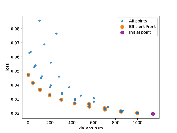
Figure 1: Efficient front and candidate solutions after 5 iterations with Algorithm 1, on the CNN model that is presented in Chapter 5. Note that we only ran 5 iterations to reduce the number of points for illustration purposes.

3.3 Main algorithm

We have now covered all components of our algorithm for improving robustness and finding an improved solution to (6). The algorithm is presented as pseudo-code in Algorithm 1. In this algorithm, we use a maximum number of iterations $M$ as the stopping criteria. This is motivated by the fact that we are searching for an approximate solution to (6), and limiting the number of iterations –and by extension the computational burden – seems reasonable. Increasing the number of iteration generally produce better results, although the main improvements are often achieved within the first 15-20 iterations.

Data: Pre-trained model parameters $\hat{w}$, $0<\omega<1$, the maximum iterations number $M$, an adversarial dataset $\mathcal{X}_{\text{adv}}$;

Output: $w$;

$\mathcal{W}_{t}\leftarrow\{w_{0}\}$ # Initialize the solutions pool;

$\mathcal{W}_{cut}\leftarrow\emptyset$ # Initialize the linear cuts set;

for $k=1,\dots,M$ do

      $w^{k}\leftarrow P(w^{0},\mathcal{X}_{\text{adv}},\mathcal{W}_{cut})$ # solving (13);

      

      $\mathcal{W}_{cut}\leftarrow\mathcal{W}_{cut}\cup w^{k}$;

       $\mathcal{W}_{t}\leftarrow\mathcal{W}_{t}\cup\{\alpha w^{k}+(1-\alpha)w^{0}\mid\forall\alpha=0.1,\dots,1\}$

      # Line search to expand the solutions pool;

      

end for

$w\leftarrow\operatorname*{arg\,min}_{w\in\mathcal{W}_{t}}\{\omega\tilde{\ell}(w)+(1-\omega)\tilde{V}(w,\mathcal{X}_{adv})\}$;

Algorithm 1 The Cutting-plane based Adversary-Correction Algorithm

In the next section, we describe some implementation details and how we can find an approximate solution to (13) in order to speed up the computations for larger neural networks.

4 Implementation details

The whole pipeline of the numerical experiment, e.g., the data preparation process, neural network training, and optimization modeling, are implemented on a MacBook Pro with an Apple M2 Pro CPU, 10 cores, and 32 GB memory. We trained neural networks using Pytorch 2.2.1 and the optimization problems are solved using Gurobi 11.0.1.

For larger neural networks, with over $10^{5}$ parameters, and with larger sets$\mathcal{X}_{\text{adv}}$ and $\mathcal{W}_{cut}$, it can become computationally costly to solve (13). To tackle the increasing computational complexity and speed-up the computations, (13) is solved by fixing a subset of variables and iterating in a block coordinate descent fashion.

An important realization is that we do not need an optimal solution to the convex QP problem (13). Instead, we need to obtain a feasible solution – ideally with an objective value close to the optimum. For this purpose, we propose a simple block coordinate optimization algorithm. The algorithm is designed for problems of the type

$$\min\leavevmode\nobreak \|w-\hat{w}\|_{2}^{2}$$ (20)

s.t. $$w\in\mathcal{L}\subset\mathbb{R}^{N},$$

where $\mathcal{L}$ is defined by linear constraints. We start by optimizing over a subset of variables and keep the other variables fixed to their corresponding values in the initial state $\hat{w}$. If the problem is feasible, we can update the solution as the initial state, and optimize over a new subset of variables. If the first selection of subset resulted in an infeasible problem, one could increase the size of the subset of variables that are optimized over or simply select a new subset. However, in practice, we never encountered a case when fixing variables and optimizing over a subset resulted in an infeasible problem. Partly because there are relatively few constraints compared to the number of variables, and partly because we still kept a large number of variables that we optimized over.

This block coordinate optimization process is simple, but there is one aspect that deserves a more detailed discussion. Let $J_{v}$ denote the subset of variables that we optimize over in each step. When updating the subsets of variables $J_{v}$ one should be careful and ensure that there is an overlap with the previous subset of variables. This is described in the following proposition.

Proposition 1.

Assume that the variables with indices $\{1,\dots,N\}\setminus J_{v}$ in (20) are fixed to their corresponding values in $\hat{w}$ and the resulting problem is feasible with a minimizer denoted by $\bar{w}$. Then by selecting any new subset of variables $J_{v}^{+}$, such that $J_{v}\cap J_{v}^{+}=\emptyset$, we cannot obtain a better solution by optimizing over the variables $J_{v}^{+}$ and fixing the rest to $\bar{w}$.

Proof.

As $J_{v}^{+}\subset\{1,\dots,N\}/J_{v}$, it is clear that $\bar{w}_{i}=\hat{w}_{i}\ \ \forall i\in J_{v}^{+}$. As we assumed that the problem was feasible by optimizing over the variables $J_{v}$, we know that $\bar{w}\in\mathcal{L}$. Furthermore, with $w_{i}=\bar{w}_{i}$ holds for all $i\in J_{v}$, $\bar{w}$ will remain the optimal solution for $w_{i}\leavevmode\nobreak\ \forall i\in J_{v}^{+}$ , as $w_{i}=\hat{w}_{i}\leavevmode\nobreak\ \forall i\in J_{v}^{+}$ minimizes their contribution to the objective. ∎

From the proposition, it is clear that we need to keep an overlap between the subsets of variables we optimize; Otherwise, we can get stuck in a potentially suboptimal solution. The algorithm is presented as pseudo-code in Algorithm 2.

Data: The feasible set $\mathcal{L}$, the variable index $I:=\subset\{1,\dots,N\}$, the fixed-ratio $0<p<1$, the maximum iterations number $T$, initial state $\hat{w}\in\mathbb{R}^{N}$;

Output: $w$;

$J_{0}\leftarrow\emptyset$;

$w^{0}\leftarrow\hat{w}$;

$J_{v}\leftarrow j_{1},\dots,j_{(1-p)|I|}\sim U(I)$ # Uniformly sample $(1-p)|I|$ indices from $I$;

for $k=1,\dots,T$ do

       $w^{k}\leftarrow\operatorname*{arg\,min}\{\|w-\hat{w}\|^{2}_{2}\mid w\in\mathcal{L}\subset\mathbb{R}^{N},w_{j}=w^{k-1}_{j},\leavevmode\nobreak\ \forall j\notin J_{v}\cup J_{0}\}$;

       $J\leftarrow I/(J_{v}\cup J_{0})$ ;

       $J_{0}\leftarrow j_{1},\dots,j_{(1-p)|I|/2}\sim U(J_{v}\cup J_{0})$ #Keep half of the selected indices from $J$;

      

      $J_{v}\leftarrow j_{1},\dots,j_{(1-p)|I|/2}\sim U(J)$ #Re-select variables to optimize;

      

end for

Algorithm 2 Alternating Approximation Algorithm for QP (20)

The selection of the fixing ratio is a trade-off between computational efficiency and approximation quality. Primary results show that even when fixing more than 50% of variables good solutions could be obtained after only a few iterations.

For the neural networks, we use a slightly more tailor-made selection strategy for selecting the variables to optimize in each step. We always keep the bias of each node as a variable, and we randomly select a proportion of variables in each layer. This ensures some flexibility to the optimization problem as the output of each node can be adjusted.

For the larger neural network ResNet8, we tackle the complexity of (20) by fixing 80% of the weight variables in each layer while keeping all the bias variables free. We performed an initial test varying the number of maximum iterations $T$, and in the end decided on using $T=1$ allowing for more iterations did not lead to any clear improvements. Although it could lead to better solutions to the QP problem (20), it did not result in final neural network with better properties. Keep in mind, for Algorithm 1, we only need a feasible solution to the QP problem (20), and a solution with a slightly lower objective will not necessarily perform better in reducing $\ell(w)$ and $V(w,\mathcal{X}_{\text{adv}})$.

For the other neural networks we did not use Algorithm 2, as we could directly solve (20) using Gurobi.

5 Computational experiments

We illustrate the performance of the fine-tuning method Alg. 1 for 2 benchmark datasets with different complexity.

• MNIST [4]: A dataset of handwritten digits of numbers 0 to 9, with each image of 28x28 pixels. The MNIST database contains 60,000 training images and 10,000 testing images. In the reprocessing, the pixel values of each image are scaled to between $0$ and $1$.

• CIFAR10 [1]: A dataset of 32x32 color images in 10 classes, i.e., airplanes, cars, birds, cats, deer, dogs, frogs, horses, ships, and trucks. There are 50,000 training images and 10,000 test images. In the preprocessing, each image is random cropped with reflection padding of size $4$, flipped horizontally with probability of $0.5$, and normalized with mean $(0.4914,0.4822,0.4465)$ and standard deviation $(0.2023,0.1994,0.2010)$.

We generate the adversarial dataset $\mathcal{X}_{\text{adv}}$ from the training dataset by the projected gradient descent (PGD) method [17] implemented with the Python library CleverHans [19], following the configurations similar as in [17]:

• MNIST: run $50$ iterations of projected gradient descent as our adversary, with a step size of $0.01$, $\ell_{\infty}$-norm with radius $0.1$.

• CIFAR10: run $3$ iterations of projected gradient descent with a step size of $3/255$, $\ell_{\infty}$-norm with radius $8/255$.

To measure the robustness of neural networks, we test their accuracy on adversarial datasets generated by PGD, and the Fast Gradient Sign Method (FGSM) [8] from CleverHans using the default test dataset. The configuration for PGD is the same as for the training process, and the configuration for FGSM has the same radius with $\ell_{\infty}$ norm.

We choose to use different architectures for each dataset. For the MNIST dataset, we choose convolutional neural networks with two sizes:

• CNNLight: A ConvNet architecture with a smaller size, which includes 2 convolutional layers, with 8 and 16 channels (each with a stride of 2, to decrease the resolution by half without requiring max pooling layers), and 2 fully connected layers stepping down to 50 and then 10 (the output dimension) hidden units, with ReLUs following each layer except the last. The total number of trainable parameters is 40908.

• CNN: A ConvNet architecture that includes 2 convolutional layers, with 16 and 32 channels (each with a stride of 2, to decrease the resolution by half without requiring max pooling layers), and 2 fully connected layers stepping down to 100 and then 10 (the output dimension) hidden units, with ReLUs following each layer except the last. The total number of trainable parameters is 162710.

For CIFAR10, we choose the residual network due to the increasing complexity of the image:

• ResNet8: An initial convolutional layer with 16 channels, followed by 3 groups of residual blocks. Each group contains 2 convolutional layers, which has 16, 32 channels (with a stride of 2 for downsampling), and 64 channels (also with a stride of 2 for downsampling) respectively. Finally, the model has an adaptive average pooling layer followed by a fully connected layer of 64x10. The residual connections are from conv1 to conv3, conv3 to conv5, and conv5 to conv7. The total number of trainable parameters is 174970.

5.1 Accuracy for MNIST

Table 1 and  2 present the results of fine-tuned CNNLight and CNN on MNIST dataset by (1) with different configurations. We present the accuracy on test dataset $\{x_{n},y_{n}\}_{test}$ and the robustness (i.e., accuracy on FGSM and PGD) with the number of adversarial datapoints, i.e., $|\mathcal{X}_{\text{adv}}|$, of $\{10,20,30,40,50\}$, and $\omega$ of $\{0,0.2,0.4\}$.

All the experiments are set up with $M=20$, which is adequate to reduce $V(\mathcal{G}(\mathcal{X}_{\text{adv}}))$ below a threshold $0.5$ in preliminary tests for CNNLight and CNN.

In Table 1, the performance of the pre-trained model (i.e., $|\mathcal{X}_{\text{adv}}|=0$) is presented as a baseline. The best result for each $|\mathcal{X}_{\text{adv}}|$ is marked in bold. The results show that the accuracy of MNIST drops less than 1 point while the accuracy on FGSM and PGD increases significantly. The accuracy on FGSM (resp. PGD) is improved from 12.38 % (resp. 3.74%) to 59.80 % (resp. 43.56%) with only $|\mathcal{X}_{\text{adv}}|=10$; With $|\mathcal{X}_{\text{adv}}|=50$, the accuracy on FGSM (resp. PGD) reaches 70.83% (resp. 62.28%). We present the results with $\omega$ of $\{0,0.2,0.4\}$ to provide some insight into how it affects the results. When $\omega=0.4$, the loss of the fine-tuned model is slightly higher than the baseline, but the accuracy on $\{x_{n},y_{n}\}_{test}$ remains the same. While decreasing the $\omega$ from $0.4$ to $0.2$ or $0$, the accuracy on FGSM and PGD increases but the MNIST accuracy drops.

Table 2 shows the fine-tuned CNN has higher accuracy on all different datasets compared to CNNLight; The accuracy on FGSM (resp. PGD) is improved from 15.67 (resp. 4.02%) to 61.54 % (reps. 45.87 %) with $|\mathcal{X}_{\text{adv}}|=10$, and further reaches 70.83% (resp. 62.28%) with $|\mathcal{X}_{\text{adv}}|=50$. It shows a similar pattern with various $\omega$.

Both tables show that the loss on $\mathcal{X}_{train}$ and accuracy on $\mathcal{X}_{test}$ are kept close to the pre-trained model. At the same time, the fine-tuning process can achieve an improvement of at least 40 points on the adversarial dataset even only with $\mathcal{X}_{adv}=10$. As $\mathcal{X}_{adv}$ increases to $50$, the improvements are further enlarged with at least 10 more points. This shows how a small number of adversarial data can be exploited to improve the robustness of our approach.

$|\mathcal{X}_{\text{adv}}|$	$\omega$	MNIST		Adversary acc.(%)
		loss	acc.(%)	FGSM	PGD
0		0.0516	97.81	12.38	3.74
10	0	0.0644	97.52	58.02	42.77
	0.2	0.0603	97.68	59.80	43.56
	0.4	0.0587	97.69	57.09	37.95
20	0	0.0685	97.65	67.83	56.08
	0.2	0.0670	97.51	66.67	55.55
	0.4	0.0619	97.64	61.65	45.48
30	0	0.0650	97.70	68.53	59.53
	0.2	0.0611	97.68	70.19	61.17
	0.4	0.0579	97.79	65.55	52.06
40	0	0.0668	97.66	69.35	61.05
	0.2	0.0610	97.89	69.44	60.15
	0.4	0.0573	97.92	64.96	50.99
50	0	0.0622	97.82	70.83	62.39
	0.2	0.0602	97.90	69.10	59.08
	0.4	0.0571	97.89	63.02	45.90

Table 1: CNNLight with $M=20$, various $|\mathcal{X}_{\text{adv}}|$ and $\omega$.

$|\mathcal{X}_{\text{adv}}|$	$\omega$	MNIST		Adversary acc.(%)
		loss	acc.(%)	FGSM	PGD
0		0.0197	98.55	15.67	4.02
10	0	0.0354	98.19	59.49	43.76
	0.2	0.0269	98.46	61.54	45.73
	0.4	0.0269	98.46	61.54	45.87
20	0	0.0276	98.54	63.84	49.84
	$0.2$	0.0276	98.54	63.84	49.84
	$0.4$	0.0252	98.53	58.60	39.71
30	0	0.0296	98.31	70.92	58.87
	$0.2$	0.0268	98.39	71.65	59.35
	$0.4$	0.0255	98.49	65.65	48.58
40	0	0.0293	98.37	72.16	62.23
	$0.2$	0.0289	98.42	73.99	63.74
	$0.4$	0.0260	98.55	68.47	53.98
50	0	0.0310	98.44	73.79	64.33
	0.2	0.0290	98.46	74.77	65.94
	0.4	0.0262	98.52	71.24	57.70

Table 2: CNN models found with $M=20$, various $|\mathcal{X}_{\text{adv}}|$ and $\omega$.

5.2 Accuracy on CIFAR10

Table 3 presents the fine-tuning results of ResNet8 on CIFAR10. Compared to MNIST dataset, CIFAR10 is a more complicated dataset and a larger model is needed to achieve a decent accuracy. The pre-trained ResNet8 has an prediction accuracy of 82.79% on CIFAR10 and 33.39 % and 30.50 % on adversarial data generated by FGSM and PGD. After the fine-tuning process with $|\mathcal{X}_{\text{adv}}|$ up to 50, the accuracy on FGSM and PGD increase up to 42.35 % and 43.86%.

Similarly as in Table 1 and 2, even using only 10 adversarial data can achieve a noticeable improvement in adversarial data classification. Even thought the growing pace is slower, the improvement is further enlarged when $\mathcal{X}_{adv}$ is included in the fine-tuning process. Initially the accuracy after fine-tuning increases when using more adversarial data, but the best results are found when $|\mathcal{X}_{\text{adv}}|=40$. This is because, as the size of the QP grows, more iterations are needed to reduce the violation of $\mathcal{G}\mathcal{X}_{\text{adv}})$ and further improvements are halted by our choice of $M=20$.

$|\mathcal{X}_{\text{adv}}|$	$\omega$	CIFAR10		Adversary acc.(%)
		loss	acc.(%)	FGSM	PGD
0		0.44	82.79	33.39	30.50
10	0	0.46	82.71	36.31	35.97
	0.2	0.46	82.20	36.71	36.36
	0.4	0.44	82.64	35.79	34.95
20	0	0.49	81.49	38.12	39.20
	0.2	0.46	81.92	40.99	42.19
	0.4	0.46	82.57	40.14	41.25
30	0	0.50	81.24	40.93	42.57
	0.2	0.46	82.19	39.67	40.52
	0.4	0.46	82.09	40.84	42.22
40	0	0.47	82.18	42.35	43.86
	0.2	0.46	82.56	41.29	43.26
	0.4	0.46	82.66	41.59	43.18
50	0	0.46	82.34	41.36	43.50
	0.2	0.46	82.12	41.12	43.12
	0.4	0.45	83.16	39.69	40.86

Table 3: ResNet8 models found with various $|\mathcal{X}_{\text{adv}}|$, $M=20$ is used to for the combined optimization.

5.3 Computational Efficiency

The fine-tuning process Algorithm 1 includes iteratively solving a growing QP problem, evaluating intermediate neural networks, and extracting the gradient information in order to generate auxiliary linear constraints. Table 4 presents the running time of solving each QP problem under various conditions, and the evaluation time of computing loss on the training dataset for neural networks with different architectures, with the aim of providing insights into the performance of each component. We break down the running time into two categories (i.e., optimization-related and evaluation-related) to further analyze the computational efficiency of this algorithm. The optimization-related computation consists of the time it takes to both construct the QP problems, and to solve them using Gurobi. The evaluation-related computation refers to the evaluation of the neural networks in order to access the gradient information.

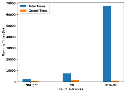
(a) $|\mathcal{X}_{\text{adv}}|=10$

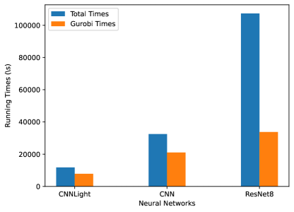
(b) $|\mathcal{X}_{\text{adv}}|=50$

Figure 2: Total running times

Table 2 illustrate the total fine-tuning time and optimization-related time (e.g., Gurobi running times) for different neural networks architectures. For CNNLight, the total fine-tuning time is between 2623.46 sec and 11763.83 sec where the number of adversarial datapoints (i.e., $|\mathcal{X}_{\text{adv}}|$) are between 10 and 50. The total optimization-related time lies between 624.37 sec and 7830.74 sec. For CNN, the total running time is between 7501.90 sec and 32514.06 sec for $|\mathcal{X}_{\text{adv}}|$ between 10 and 50, and the total optimization-related time is between 1699.61 sec and 21051.21 sec. For ResNet8, due to the increasing size of the neural network, the total running is between 67518.09 sec to 107319.27 sec with $|\mathcal{X}_{\text{adv}}|$ from 10 to 50, where the total optimization-related time is between 979.31 sec to 33763.22 sec respectively.

The above results are from experiments conducted only on CPU, and they shown that the optimization-related computations only accounts for 20% - 65% of the total execution time for CNNs, and accounts for even less, 1% - 31%, when considering the larger neural networks, i.e., ResNet8.

We want to stress that the computations could be sped up significantly. Many of the computations can easily be run in parallel, as we discuss more in detail in the following subsections. Additionally, we have not used the best machine for running experiments of this type. As an example, the time for evaluating the neural networks could potentially be reduced by a factor of 10 (as the main evaluations could be run in 10 parallel processes). We have not investigated this further, as our main goal with this paper is to provide a proof of concept – that this approach can successfully be used in order to improve the robustness of neural networks. We believe the numerical results clearly show the feasibility and value of the proposed method.

The optimization-related computation

The difficulty of solving QP problems directly relates to the number of constraints and variables. In our setting, the number of variables is proportional to the size of the neural network. The number of constraints is proportional to the size of $\mathcal{W}_{cuts}$ and $\mathcal{X}_{\text{adv}}$, which is reflected by the neural network type, iteration number $k$ and $|\mathcal{X}_{\text{adv}}|$ respectively in Table 4.

It is shown that the QP solving times are similar for different architectures with $\mathcal{X}_{\text{adv}}$, but are more impacted by the size of neural network when $k=20$. This pattern indicates the bottleneck of solving QPs efficiently is caused by the size of neural network. Due to the nature of large-sized neural networks and the formulation of (13), the number of variables is relatively large compared to the number of constraints. Therefore, we believe it could be solved more efficiently with a tailor-made implementation of a dual algorithm that could also benefit from warm-starts.

The evaluation-related computation

The evaluation times of the loss function on the training dataset for CNNLight, CNN and ResNet8 is shown in Table 4 to reflect how the level of evaluation-related computational cost changes with the size of neural networks grows. We emphasize here that the execution times of evaluating the neural networks depends on the total number of iterations, and the partition of stepsizes for the line search.

For CNNLight and CNN, the loss evaluation time for a single execution is relatively small. Still, the accumulated time – considering a total 20 iterations and 10 line search stepsizes – is still significant. To improve the efficiency, a more finely partitioned line search could be applied only in later iterations, since the high-quality candidate solutions are not found in the early stages. Moreover, the evaluation of the neural networks can be parallelized for better computational efficiency, especially for ResNet8, where a single execution of evaluating the loss can take $\sim$ 270 sec. All points of the line search could be evaluated fully in parallel, and this could greatly speed up the computations. We could also evaluate the loss function on smaller batches to reduce computational cost in this category.

	QP (Gurobi)			Eval. of loss
	$|\mathcal{X}_{\text{adv}}|$	$k$	time	Dataset	time
CNNLight	10	1	1.10	MNIST	$\sim$ 0.07
	10	20	69.23
	50	1	10.66
	50	20	949.78
CNN	10	1	1.13	MNIST	$\sim$ 9.39
	10	20	69.24
	50	1	30.19
	50	20	3089.63
ResNet8	10	1	2.09	CIFAR10	$\sim$ 275.92
	10	20	96.53
	50	1	15.98
	50	20	4130.36

Table 4: Running times in each component

6 Conclusion

We reformulate the robust training problem as a fine-tuning process that aims to solve an adversary-correction problem. This nonlinear problem is solved by linearization and cutting-plane framework to improve the approximation. Based on this framework, Algorithm 1 uses line search and a weighted objective function to balance the accuracy on both the test- and adversarial datasets. We illustrate the performance of our method by numerical experiments with pre-trained models of various sizes and architectures. The numerical results show that we can significantly improve the robustness of CNNs and ResNet8 even with as little as 10 adversarial data points in the fine-tuning process, and obtain even greater improvements using more adversarial data. Our method shows a new direction for robust training of neural networks, and the numerical results support that the adversarial correction problem is a sound approach for fine-tuning neural networks to improve robustness.

7 Acknowledgment

The authors gratefully acknowledge funding from Digital Futures and the 3.ai Digital Transformation Institute project AI techniques for Power Systems Under Cyberattacks.

References

- Alex, [2009] Alex, K. (2009). Learning multiple layers of features from tiny images. https://www. cs. toronto. edu/kriz/learning-features-2009-TR. pdf.
- Aspman et al., [2024] Aspman, J., Korpas, G., and Marecek, J. (2024). Taming binarized neural networks and mixed-integer programs. Proceedings of the AAAI Conference on Artificial Intelligence, 38(10):10935–10943.
- Botoeva et al., [2020] Botoeva, E., Kouvaros, P., Kronqvist, J., Lomuscio, A., and Misener, R. (2020). Efficient verification of relu-based neural networks via dependency analysis. In Proceedings of the AAAI Conference on Artificial Intelligence, volume 34, pages 3291–3299.
- Deng, [2012] Deng, L. (2012). The mnist database of handwritten digit images for machine learning research. IEEE Signal Process. Mag., 29(6):141–142.
- Eichfelder, [2021] Eichfelder, G. (2021). Twenty years of continuous multiobjective optimization in the twenty-first century. EURO Journal on Computational Optimization, 9:100014.
- Eykholt et al., [2018] Eykholt, K., Evtimov, I., Fernandes, E., Li, B., Rahmati, A., Xiao, C., Prakash, A., Kohno, T., and Song, D. (2018). Robust physical-world attacks on deep learning visual classification. In Proceedings of the IEEE conference on computer vision and pattern recognition, pages 1625–1634.
- Fischetti and Jo, [2018] Fischetti, M. and Jo, J. (2018). Deep neural networks and mixed integer linear optimization. Constraints, 23(3):296–309.
- Goodfellow et al., [2014] Goodfellow, I. J., Shlens, J., and Szegedy, C. (2014). Explaining and harnessing adversarial examples. arXiv preprint arXiv:1412.6572.
- Huang et al., [2018] Huang, X., Kroening, D., Kwiatkowska, M., Ruan, W., Sun, Y., Thamo, E., Wu, M., and Yi, X. (2018). Safety and trustworthiness of deep neural networks: A survey. arXiv preprint arXiv:1812.08342, page 151.
- Katz et al., [2017] Katz, G., Barrett, C., Dill, D. L., Julian, K., and Kochenderfer, M. J. (2017). Reluplex: An efficient smt solver for verifying deep neural networks. In Computer Aided Verification: 29th International Conference, CAV 2017, Heidelberg, Germany, July 24-28, 2017, Proceedings, Part I 30, pages 97–117. Springer.
- Kelley, [1960] Kelley, Jr, J. E. (1960). The cutting-plane method for solving convex programs. Journal of the society for Industrial and Applied Mathematics, 8(4):703–712.
- Kurakin et al., [2016] Kurakin, A., Goodfellow, I., and Bengio, S. (2016). Adversarial machine learning at scale. arXiv preprint arXiv:1611.01236.
- LeCun et al., [2015] LeCun, Y., Bengio, Y., and Hinton, G. (2015). Deep learning. nature, 521(7553):436–444.
- Liao et al., [2018] Liao, F., Liang, M., Dong, Y., Pang, T., Hu, X., and Zhu, J. (2018). Defense against adversarial attacks using high-level representation guided denoiser. In Proceedings of the IEEE conference on computer vision and pattern recognition, pages 1778–1787.
- Liu et al., [2021] Liu, A., Liu, X., Yu, H., Zhang, C., Liu, Q., and Tao, D. (2021). Training robust deep neural networks via adversarial noise propagation. IEEE Transactions on Image Processing, 30:5769–5781.
- Machado et al., [2021] Machado, G. R., Silva, E., and Goldschmidt, R. R. (2021). Adversarial machine learning in image classification: A survey toward the defender’s perspective. ACM Computing Surveys (CSUR), 55(1):1–38.
- Madry et al., [2017] Madry, A., Makelov, A., Schmidt, L., Tsipras, D., and Vladu, A. (2017). Towards deep learning models resistant to adversarial attacks. arXiv preprint arXiv:1706.06083.
- Mäkelä, [2002] Mäkelä, M. (2002). Survey of bundle methods for nonsmooth optimization. Optimization methods and software, 17(1):1–29.
- Papernot et al., [2018] Papernot, N., Faghri, F., Carlini, N., Goodfellow, I., Feinman, R., Kurakin, A., Xie, C., Sharma, Y., Brown, T., Roy, A., Matyasko, A., Behzadan, V., Hambardzumyan, K., Zhang, Z., Juang, Y.-L., Li, Z., Sheatsley, R., Garg, A., Uesato, J., Gierke, W., Dong, Y., Berthelot, D., Hendricks, P., Rauber, J., and Long, R. (2018). Technical report on the cleverhans v2.1.0 adversarial examples library. arXiv preprint arXiv:1610.00768.
- Papernot et al., [2017] Papernot, N., McDaniel, P., Goodfellow, I., Jha, S., Celik, Z. B., and Swami, A. (2017). Practical black-box attacks against machine learning. In Proceedings of the 2017 ACM on Asia conference on computer and communications security, pages 506–519.
- Qin et al., [2019] Qin, C., Martens, J., Gowal, S., Krishnan, D., Dvijotham, K., Fawzi, A., De, S., Stanforth, R., and Kohli, P. (2019). Adversarial robustness through local linearization. Advances in neural information processing systems, 32.
- Raghunathan et al., [2018] Raghunathan, A., Steinhardt, J., and Liang, P. (2018). Certified defenses against adversarial examples. In International Conference on Learning Representations.
- Ruan et al., [2018] Ruan, W., Huang, X., and Kwiatkowska, M. (2018). Reachability analysis of deep neural networks with provable guarantees. arXiv preprint arXiv:1805.02242.
- Sehwag et al., [2020] Sehwag, V., Wang, S., Mittal, P., and Jana, S. (2020). Hydra: Pruning adversarially robust neural networks. Advances in Neural Information Processing Systems, 33:19655–19666.
- Shi et al., [2021] Shi, Z., Wang, Y., Zhang, H., Yi, J., and Hsieh, C.-J. (2021). Fast certified robust training with short warmup. Advances in Neural Information Processing Systems, 34:18335–18349.
- Sosnin et al., [2024] Sosnin, P., Müller, M. N., Baader, M., Tsay, C., and Wicker, M. (2024). Certified robustness to data poisoning in gradient-based training. arXiv:2406.05670.
- Szegedy et al., [2014] Szegedy, C., Zaremba, W., Sutskever, I., Bruna, J., Erhan, D., Goodfellow, I., and Fergus, R. (2014). Intriguing properties of neural networks. arXiv preprint arXiv:1312.6199.
- Thorbjarnarson and Yorke-Smith, [2023] Thorbjarnarson, T. and Yorke-Smith, N. (2023). Optimal training of integer-valued neural networks with mixed integer programming. Plos one, 18(2):e0261029.
- Toro Icarte et al., [2019] Toro Icarte, R., Illanes, L., Castro, M. P., Cire, A. A., McIlraith, S. A., and Beck, J. C. (2019). Training binarized neural networks using mip and cp. In Principles and Practice of Constraint Programming: 25th International Conference, CP 2019, Stamford, CT, USA, September 30–October 4, 2019, Proceedings 25, pages 401–417. Springer.
- Tramèr et al., [2017] Tramèr, F., Kurakin, A., Papernot, N., Goodfellow, I., Boneh, D., and McDaniel, P. (2017). Ensemble adversarial training: Attacks and defenses. arXiv preprint arXiv:1705.07204.
- Tsay et al., [2021] Tsay, C., Kronqvist, J., Thebelt, A., and Misener, R. (2021). Partition-based formulations for mixed-integer optimization of trained relu neural networks. Advances in neural information processing systems, 34:3068–3080.
- Tsiligkaridis and Roberts, [2022] Tsiligkaridis, T. and Roberts, J. (2022). Understanding and increasing efficiency of frank-wolfe adversarial training. In Proceedings of the IEEE/CVF Conference on Computer Vision and Pattern Recognition, pages 50–59.
- Wu and Zhang, [2021] Wu, Y. and Zhang, M. (2021). Tightening robustness verification of convolutional neural networks with fine-grained linear approximation. In Proceedings of the AAAI Conference on Artificial Intelligence, volume 35, pages 11674–11681.
- Zhao et al., [2023] Zhao, S., Tsay, C., and Kronqvist, J. (2023). Model-based feature selection for neural networks: A mixed-integer programming approach. In International Conference on Learning and Intelligent Optimization, pages 223–238. Springer.
- Zügner and Günnemann, [2019] Zügner, D. and Günnemann, S. (2019). Certifiable robustness and robust training for graph convolutional networks. In Proceedings of the 25th ACM SIGKDD International Conference on Knowledge Discovery & Data Mining, pages 246–256.