Slowing and stopping the speed of sound

Abstract

Temporal interference between direct and surface-reflected paths induces large variation in the group speed of an acoustic signal between a source and receiver. This speed goes to zero when the source and receiver approach one another and are within $c\tilde{\delta t}/2$ of the surface, where $c$ is the in-situ speed of sound and $\tilde{\delta t}$ is the smallest temporal separation between the paths at which interference initiates. At greater depths, the group speed can drop by many orders of magnitude. The effect diminishes far from a receiver as the size of the delay shrinks relative the overall time of propagation. The phenomenon is of great importance for methods designed to locate sounds via time differences of arrival (TDOA) as the group speed between a sound and each receiver may differ by orders of magnitude, a phenomenon that invalidates the geometrical interpretation of location by hyperboloids. Isodiachronic geometries are required to derive valid locations. Analogous to gravitational black holes, where the speed of light is zero at the event horizon, “three-dimensional acoustical black holes” can be present at acoustical receivers.

I Introduction

Locations of underwater objects are often derived from measurements of emitted or reflected sounds. Examples include ships, submarines, torpedoes, mines, fish, explosions, implosions, earthquakes, and calling animals. Quite often, locations are derived from either the propagation time of sound or a TDOA between pairs of receivers. Propagation time and TDOA are converted to distance and difference in distance from two receivers respectively by multiplication by a speed of sound. The origins of these methods date back at least to Milne [39] where locations of underwater earthquakes were estimated from the TDOA of tsunamis at multiple locations on land. For three-dimensional spatial locations, the “three-dimensional effective speed” is defined as,

$$c_{3d}\equiv l_{1}/t_{m}\ ,$$ (1)

where $l_{1}$ is the distance of a straight-line path from source to receiver and $t_{m}$ is the measured time of arrival. This is a required input for numerous software packages deriving location of calling marine mammals with TDOA [36, 35, 24, 11, 25, 69, 3]. Yet, something surprising occurred when a program was run to compute $c_{3d}$ to locate explosive sounds in the ocean. Values of $c_{3d}$ were 50 m/s less than the in-situ speed a few hundreds of meters from the receiver. Initially thinking the phenomenon was a software bug, it was later discovered the phenomenon was caused by interference between the direct and surface-reflected paths. The direct path is the shortest and does not reflect from a boundary. The reflected path leaves the source, reflects once at the surface, then travels down to the receiver. For sources near the receiver, the peak of the first energetic arrival was delayed by interference. This increased $t_{m}$ and caused $c_{3d}$ to decrease (Eq. 1). We have not found prior discussions of a large drop of group speed due to this type of interference, though such a study may exist. If it does, the phenomenon is apparently not considered by contemporary acoustical oceanographers so is worth highlighting as its effects on the accuracy of location can be important. For example, a thorough investigation of this phenomenon demonstrates the $c_{3d}$ can drop to zero meters per second. Using correct values for the $c_{3d}$ may be necessary to obtain a reliable confidence interval of location (CIL) for the class of models whose inputs require $c_{3d}$.

Interference effects are discussed across many scientific disciplines. For a single acoustic frequency, interference near the ocean’s surface occurs due to the physics described by Lloyd [32]. However, propagation time is inherently a many frequency phenomenon since it cannot be measured with single-frequency emissions. For signals with positive bandwidth, interference affects propagation times of acoustic signals. For example, rays are a consequence of the interference of acoustical modes, each ray with its own time of propagation (e.g. Sec. 6.7.1, Brekhovskikh and Lysanov [6]). Interference is used to explain why the speed of light in a vacuum is slowed by glass and water [23] (Vol I, Chapt 31). When a gas is cooled near absolute zero, its interference properties can be manipulated to yield a group speed of 17 m/s for light [26]. Its speed can be decreased to zero meters per second by storing it in a quantum state for 1 ms [31].

The paper is organized as follows. Sec. II discusses geometrical shapes useful for understanding how interference affects propagation speed and how locations are understood when derived with TDOA. Sec. III quantifies how the speed of signal propagation is affected by interference between the direct and reflected paths. Sec. IV presents examples of the depressed speed along with quantification of its effects on the accuracy of locating sounds. A discussion appears in Sec. V.

II Locating objects with TDOA

Deriving locations using TDOA can mainly be interpreted using one of two geometries: hyperboloids or isodiachrons [51]. Both shapes are useful for understanding how interference affects location predictions as well as how it modifies the group speed of acoustic waves.

II.1 Location via hyperbolas

For two and three-dimensional models of location (2D and 3D), it is necessary to have at least four and five receivers respectively to yield a mathematically unambiguous solution for location from TDOA when measurements are made without error [48]. The TDOA,

$$\delta t=t({\bf r}_{2})-t({\bf r}_{1})\ ,$$ (2)

is transformed into the source’s difference in distance, $\delta d$, from receivers located at ${\bf r}_{1}$ and ${\bf r}_{2}$ using $\delta d=c\delta t$, where $c$ is a constant wave speed. The locus of points in space sharing this difference defines a hyperbola in 2D space or hyperboloid in 3D space [38]. Adding receivers creates additional hyperbolas or hyperboloids, whose intersections coincide at a single point with four receivers in 2D and and five receivers in 3D. The constant speed approximation can lead to large errors in practice so must be abandoned to obtain a reliable CIL [54, 34].

II.2 Location via isodiachrons

Deriving location from TDOA via hyperbolas requires multiplication of the TDOA by a constant speed (Sec. II.1). The isodiachron [51], invented to account for problems with a constant speed, is the locus of points for which the difference in propagation time is constant, allowing sound speed to differ between paths. Mathematically, its shape is defined by,

$$\delta t=\frac{l_{2}}{c_{2}}-\frac{l_{1}}{c_{1}}\ ,$$ (3)

where $c_{i}$ is the group speed of propagation along path $l_{i}$ from source to receiver number $i$ and $l_{i}$ are usually taken to be line segments. When $c_{1}=c_{2}=c$, Eq. (3) reduces to $l_{2}-l_{1}=c\delta t$, and the isodiachron becomes a hyperbola. When $c_{1}\neq c_{2}$, isodiachrons can look very different for realistic situations [51, 54]. When $c_{i}$ is independent of location, the isodiachron is class one. Otherwise it is class two [51].

III 3D effective speed and interference

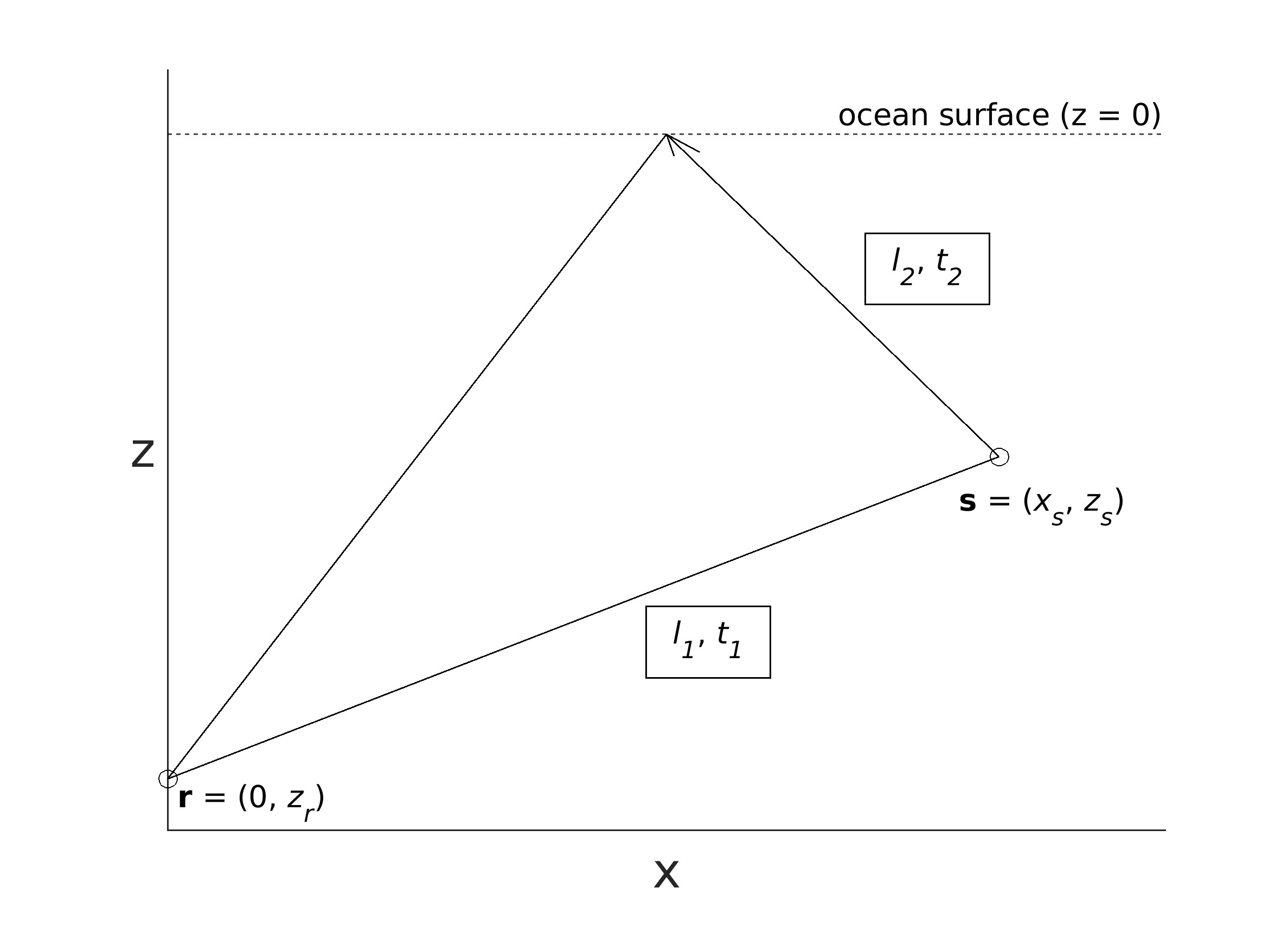
Figure 1: Sound propagates from source ${\bf s}$ to receiver ${\bf r}$ along direct and surface reflected paths with lengths, $l_{1}$ and $l_{2}$, and propagation times, $t_{1}$ and $t_{2}$, respectively.

.

The $c_{3d}$ is modified by interference over regions near an acoustic receiver, diminishing at large distances. Analytical solutions for the effects of interference are derived below for simple situations to gain intuition about where $c_{3d}$ is most impacted.

Because of Fermat’s least-time principle (p. 457-463 of Fermat [21]), the propagation time of a signal is affected by changes in path at second order, and these are ignored with respect to a curved path. Thus for short distances, the direct path is assumed to be a line segment between source and receiver while the reflected path is assumed to be two line segments: one from source to the ocean’s surface, and the other from the surface to the receiver. The angle of ray incidence at the surface is assumed to equal its angle of reflection.

The Pythagorean distance between a receiver at ${\bf r}=(0,z_{r})$ and source at ${\bf s}=(x_{s},z_{z})$ is,

$$l_{1}=|{\bf s}-{\bf r}|=\sqrt{x_{s}^{2}+(z_{r}-z_{s})^{2}}\ ,$$ (4)

where the horizontal Cartesian axis is $x$ and vertical axis, $z$, with $z$ positive up and zero at the ocean’s surface. Similarly, the length of the surface reflected path is,

$$l_{2}=\sqrt{x_{s}^{2}+(z_{r}+z_{s})^{2}}\ .$$ (5)

The z-weighted averages of sound speed along $l_{1}$ and $l_{2}$ are $c_{1}$ and $c_{2}$ respectively. The propagation times along these paths are,

$$t_{i}=\frac{l_{i}}{c_{i}}\ ;\ i=1,2\ .$$ (6)

The difference in time between the measured and direct paths is,

$$\delta t_{m}=t_{m}-t_{1}\ ,$$ (7)

where $t_{m}$ is not usually equal to $t_{2}$ in the presence of interference.

Contours of constant $c_{3d}$ can be computed from Eq. (1) given specified waveforms and knowing $\delta t_{m}$’s dependence on $c_{i}$, ${\bf r}$, and ${\bf s}$. The surfaces on which $c_{3d}$ are constant have an analytical solution assuming $c_{1}$ and $c_{2}$ are the same, and the waveforms are boxcar functions of duration $w$. The simplicity of the boxcar case stems from the reasonable assumption that $t_{m}$ is taken to be the earliest time of the largest value of the sum of the two boxcar functions, when temporal interference occurs (Fig. 2). Thus, $t_{m}=t_{2}$ (Fig. 3A) and then,

$$\delta t_{m}=t_{2}-t_{1}\ ;\ t_{2}-t_{1}\leq w\ .$$ (8)

When there is no temporal overlap, $\delta t_{m}=0$ (Fig. 2). The function, $t_{m}(t_{2}-t_{1})$ is called the “pulse interference curve” (Fig. 3).

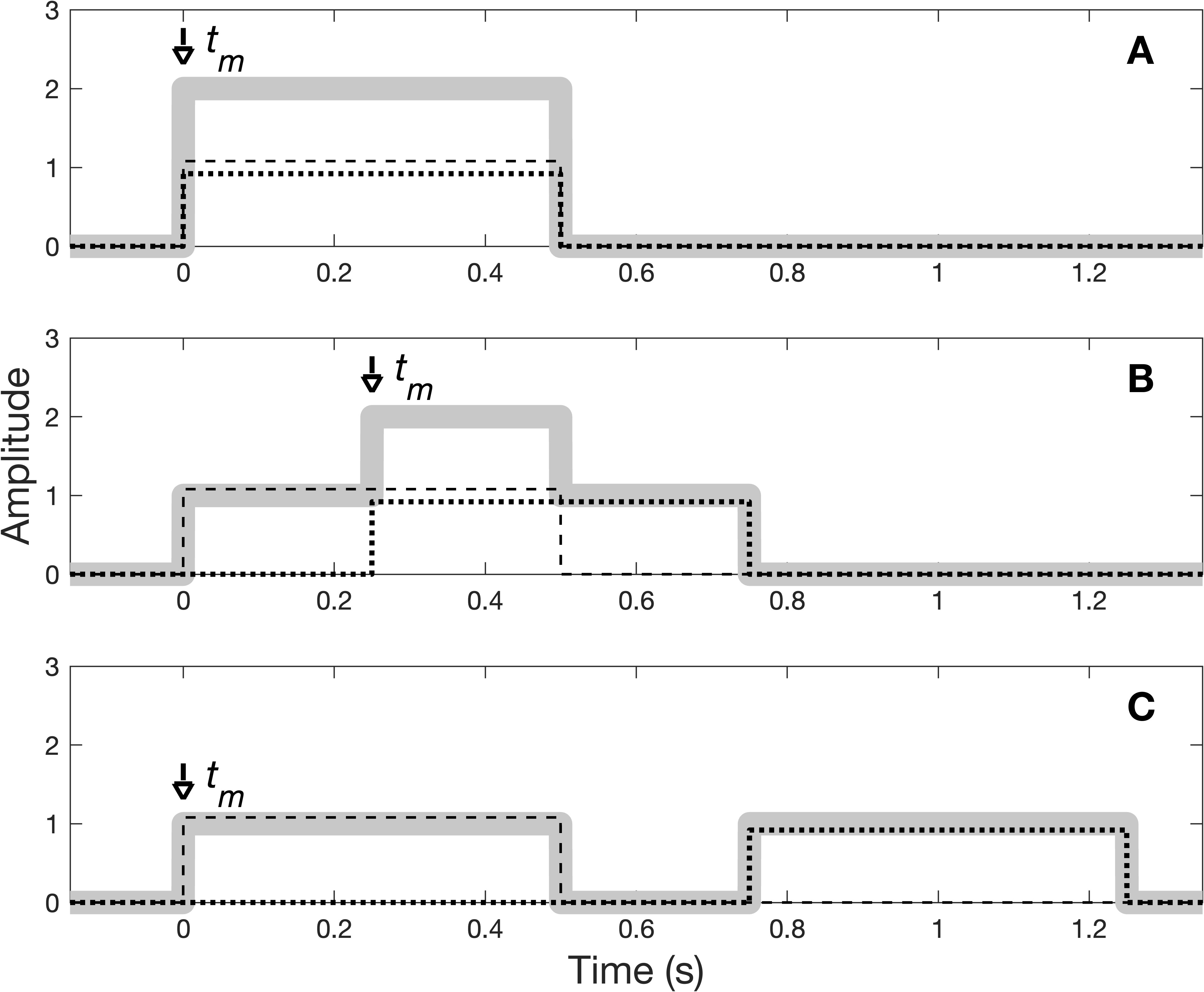
Figure 2: Measured times of arrival ($t_{m}$) based on relative arrival times of direct and reflected paths. Emitted waveforms are boxcars. A: Direct (dashed) and reflected (dotted) arrive at same time (solid gray). B: Same as A but reflected arrives later. C: Same as A but reflected arrives much later so there is no interference.

.

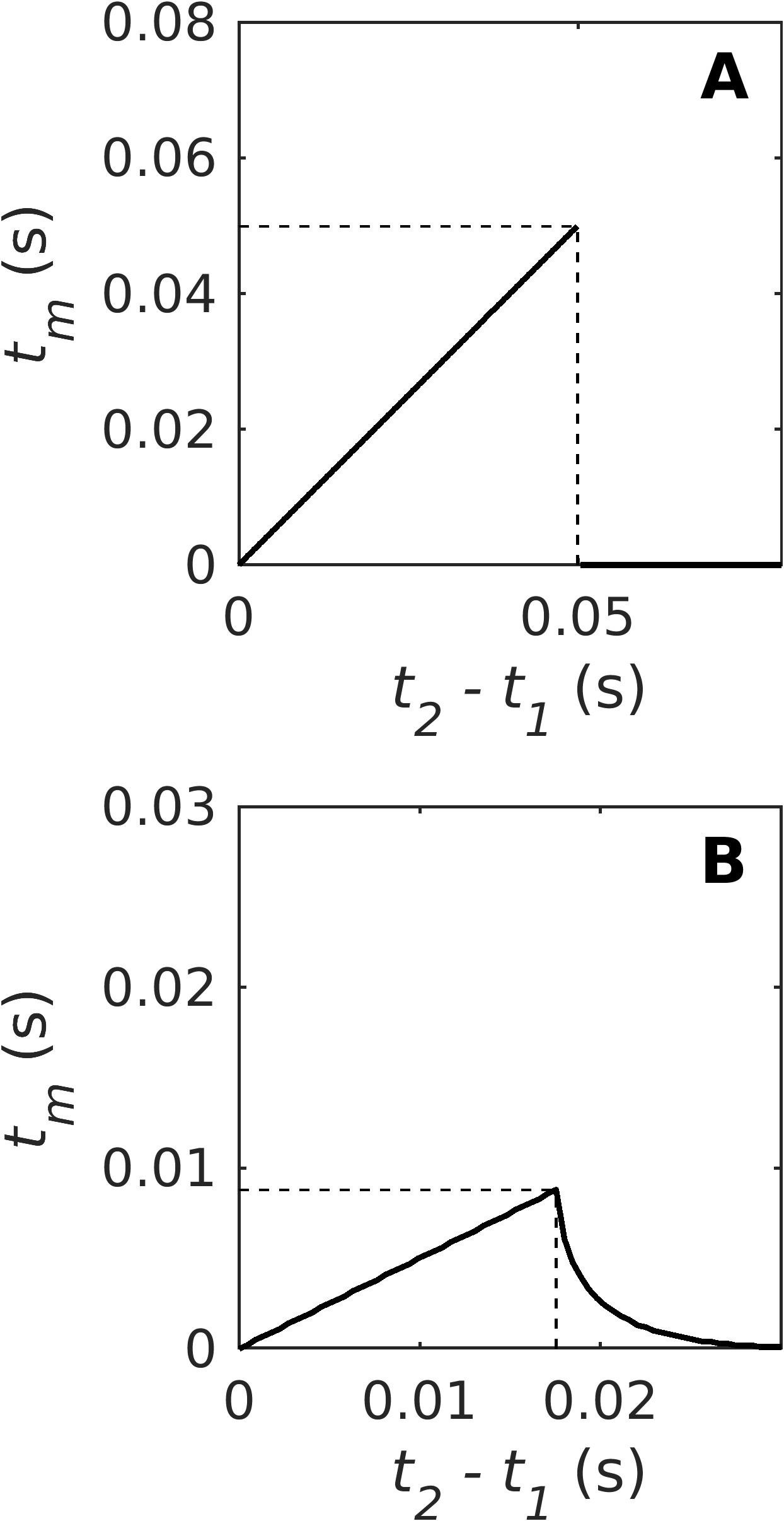
Figure 3: Pulse interference curves for boxcar (A) and exponential pulses (B). Pulse duration for boxcar is 0.05 s and $\tau=0.05$ s for exponential pulse in Eq. (32). Dashed lines indicate maximum value of $t_{m}$.

.

When interference occurs, Eq. (8) is substituted into Eq. (1) along with values for $t_{i}$ from Eq. (6) to get,

$$c_{3d}=c\frac{l_{1}}{l_{2}}\ ;\ t_{2}-t_{1}\leq w,$$ (9)

and where $c=c_{1}=c_{2}$ because the speed is spatially homogeneous. The surface on which $c_{3d}$ is constant obeys,

$$\frac{l_{1}}{l_{2}}=\frac{c_{3d}}{c}=b=\mbox{constant}\ .$$ (10)

Substituting Eqs. (4,5) into Eq. (10) yields,

$$\frac{\sqrt{x_{s}^{2}+(z_{r}-z_{s})^{2}}}{\sqrt{x_{s}^{2}+(z_{r}+z_{s})^{2}}} = b$$ (11)

$$(1-b^{2})x_{s}^{2}+(1-b^{2})z_{s}^{2}-2(1+b^{2})z_{r}z_{s} = (b^{2}-1)z_{r}^{2}$$

$$x_{s}^{2}+z_{s}^{2}-\frac{2(1+b^{2})z_{r}}{(1-b^{2})}z_{s} = -z_{r}^{2}$$

$$x_{s}^{2}+z_{s}^{2}+gz_{s} = -z_{r}^{2}$$

$$x_{s}^{2}+(z_{s}+g/2)^{2} = g^{2}/4-z_{r}^{2}\ ;\ b\neq 1\$$ (12)

where,

$$g\equiv-\frac{2(1+b^{2})z_{r}}{1-b^{2}}\ .$$ (13)

This describes a circle with center $(0,-g/2)$ and radius,

$$\rho=(g^{2}/4-z_{r}^{2})^{1/2}=\frac{2cc_{3d}}{c^{2}-c_{3d}^{2}}|z_{r}|.$$ (14)

Real-valued solutions exist when $\rho\geq 0$. When $b=1$, there is no reflected path since Eq. (10) yields $l_{1}=l_{2}$. Note $g\geq 0$ because $b<1$ and $z_{r}\leq 0$.

Eq. (9) implies $c_{3d}$ approaches zero when $l_{1}$ approaches zero, subject to interference occurring. Since $c_{3d}$ can only be zero when $l_{1}$ is zero, so the source and receiver must be co-located. If they are too deep, interference no longer occurs between the direct and reflected paths. The maximum receiver depth at which interference can occur with $c_{3d}=0$ equals,

$$d_{c}=cw/2\ ;\ \mbox{for boxcar pulses}\ ,$$ (15)

and is called the critical depth. If the emitted pulse is not a boxcar function, $w$ is replaced by,

$$d_{c}=c\tilde{\delta t}/2\ ,$$ (16)

where $\tilde{\delta t}$ is the minimum time delay, exceeding zero, yielding insignificant interference between direct and reflected signals.

III.1 Receiver below critical depth: minimum $c_{3d}$

When the in-situ speed of sound is a constant, $c$, the emitted pulse is a boxcar function, and the receiver’s depth exceeds $d_{c}$, $c_{3d}>0$ and its minimum, $\check{c}_{3d}$, can be derived analytically. Surfaces of constant $c_{3d}$ in the $x-z$ plane are circles (Eq. 12). The receiver is at $(0,z_{r})$ and the minimum speed occurs when $c_{3d}\equiv l_{1}/t_{m}$ is minimum, $\check{c}_{3d}$. Thus, the location of the source is chosen to minimize $l_{1}$ and maximize $t_{m}$. The maximum delay between measured and direct path times is given by Eq. (7) so $t_{m}$ is maximum when $\delta t_{m}$ is $\widehat{\delta t}_{m}$, its maximum value. So $\check{c}_{3d}$ corresponds to minimum $l_{1}$ and $\widehat{\delta t}_{m}$. occurring when,

$$l_{2}-l_{1}=c{\widehat{\delta}t}_{m}\ .$$ (17)

The simplest geometry for solutions of $l_{i}$ is to place the source vertically above the receiver on the circle on which $\check{c}_{3d}$ occurs. Then,

$$l_{1}=z_{s}-z_{r}\ ,$$ (18)

because the source is above the receiver, and,

$$l_{2}=l_{1}-2z_{s}\ ,$$ (19)

(Fig. 4). Solving Eq. (17) for $l_{2}$ and substituting it into Eq. (19) yields the vertical coordinate of the source,

$$z_{s}=\frac{-c{\widehat{\delta}t}_{m}}{2}\ .$$ (20)

From Eq. (18),

$$l_{1}=-c{\widehat{\delta}t}_{m}/2-z_{r}\ .$$ (21)

Since the measured time of arrival is,

$$t_{m}=l_{1}/c+{\widehat{\delta}t}_{m}\ ,$$ (22)

the minimum value of $c_{3d}$ is,

$$\check{c}_{3d}=l_{1}/t_{m}=-(c{\widehat{\delta}t}_{m}/2+z_{r})/(l_{1}/c+{\widehat{\delta}t}_{m})\ .$$ (23)

Use $l_{1}$ from Eq. (21) in this to get,

$$\check{c}_{3d}=c\frac{z_{r}+\widehat{\delta t}_{m}/2}{z_{r}-\widehat{\delta t}_{m}/2}\ .$$ (24)

When $c$ is not constant or when the emitted pulse is not a boxcar, $\check{c}_{3d}$ is computed numerically.

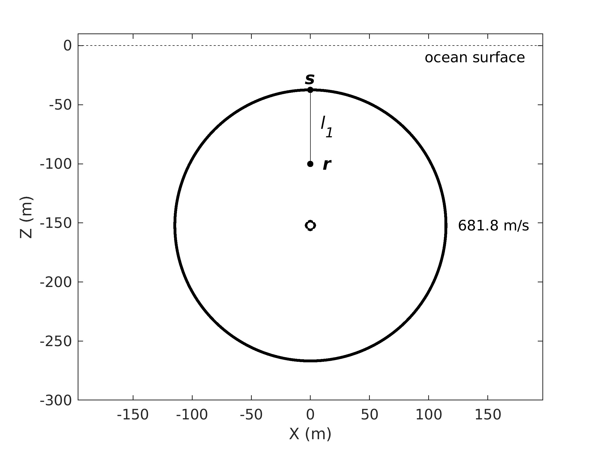
Figure 4: Source and receiver at $(x,z)$ Cartesian coordinates (0,-37.5) and (0,-100) m respectively separated by distance $l_{1}$ in ocean with constant in-situ speed of sound of 1500 m/s. Source emits a boxcar function pulse of duration 0.05 s. Because receiver is below critical depth, $d_{c}=0.05\ \mbox{s}\times 1500/2\ \mbox{m/s}=37.5$ m, minimum possible effective speed, $\check{c}_{3d}$, exceeds zero and equals 681.8 m/s anywhere on circle (Eq. 24).

III.2 Receiver below critical depth: interference boundary

There are places where interference does not occur, and the “interference-boundary” separates them from regions where interference occurs. The boundary can be computed analytically for a simple case. It satisfies,

$$\frac{l_{2}}{c_{2}}-\frac{l_{1}}{c_{1}}={\tilde{\delta}t}\ .$$ (25)

This defines an isodiachron (Sec. II). When $c_{1}=c_{2}=c$, Eq. (25) reduces to $l_{2}-l_{1}=c{\tilde{\delta}t}$; a hyperbola (Sec. II, Fig. 5). If the receiver is at or above the critical depth, all regions are subject to interference.

Figure 5: Hyperbola separates regions where interference does and does not occur between direct and reflecting paths, assuming the in-situ speed of sound is 1500 m/s and the emitted pulse is a boxcar function of duration 0.02 s. Black dots are the hyperbola’s foci. Receiver at 50 m depth is below the critical depth, $d_{c}=wc/2=0.02\ \mbox{s}\ \times\ 1500\ \mbox{m/s}=15$ m. Horizontal distance to boundary, $d_{b}$, from Eq. (26).

.

When a receiver is below the critical depth, it is useful to compute the horizontal distance, $d_{b}$, between a vertical line passing through the receiver to the interference boundary. After many algebraic steps (not shown), Eq. (25) yields,

$$d_{b}=\sqrt{\frac{c^{2}{\tilde{\delta}t}^{2}}{4}+\frac{4z_{r}^{2}z_{s}^{2}}{c^{2}{\tilde{\delta}t}^{2}}-z_{s}^{2}-z_{r}^{2}}\ \ ;\ z_{r}<-d_{c}\ \ z_{s}\leq d_{c}\ ,$$ (26)

where $d_{c}$ is defined in Eq. (16) and $d_{b}$ is $x_{s}$ for this case. The horizontal distance, $d_{b}$, is zero when $z_{s}=-c\tilde{\delta t}/2=d_{c}$. For boxcar pulses, $c_{3d}$ is minimized at the interference boundary because $t_{m}$ is most delayed when interference initiates (Fig. 2). So, $d_{b}$ is the distance to $\check{c}_{3d}$, where there is a discontinuity in the group speed. For exponential pulses, there is no discontinuity. It was found empirically that replacing $\tilde{\delta}t$ with the relative time, $t_{2}-t_{1}$, corresponding to the maximum value of $t_{m}$, in Eq. (26) yielded a distance that approximately located $\check{c}_{3d}$, and was well beyond the interference boundary (not shown).

III.3 Interference and distance of influence

Effects of interference on the $c_{3d}$ diminish at large distances from the receiver because the corresponding time shift becomes small compared with the propagation time. This is quantified using,

$$\delta c\equiv c_{1}-c_{3d}=\frac{l_{1}}{t_{1}}-\frac{l_{1}}{t_{m}}\ ,$$ (27)

where Eqs (6) and (1) are used for $c_{1}$ and $c_{3d}$. When interference occurs, an analytical solution for $\delta c$ is derived when the in-situ speed of sound, c, is constant and the emitted pulse is a boxcar function, so $t_{m}=t_{2}$. Then

$$\delta c=l_{1}\biggl{(}\frac{1}{t_{1}}-\frac{1}{t_{2}}\biggr{)}=\frac{l_{1}\delta t}{t_{1}^{2}(1+\frac{\delta t}{t_{1}})}\ .$$ (28)

For larger times of propagation, $\delta t/t_{1}<1$, and the Taylor series expansion for Eq. (28) is,

$$\delta c=c^{2}\frac{\delta t}{l_{1}}\biggl{(}1-\frac{\delta t}{l_{1}}c+(\frac{\delta t}{l_{1}}c)^{2}+\cdots\biggr{)}\ ,$$ (29)

where $l_{1}=ct_{1}$ was used. Retaining only the leading terms in $c\delta t/l_{1}$ yields an approximate distance of influence,

$$l_{1}\sim c^{2}\frac{\delta t}{\delta c}\ .$$ (30)

For example, let $c=1500$ m/s and $\delta t=$ 0.02 s. For $l_{1}=450$ m, $\delta c=100$ m/s and when $l_{1}=1125$ m, $\delta c=40$ m/s. This shows the effect dies off with distance.

III.4 Increased $c_{3d}$

The $c_{3d}$ exceeds the direct paths’ average speed when,

$$\frac{c_{3d}}{c_{1}}=\frac{t_{1}}{t_{m}}\ >1.$$ (31)

In water, this can occur when the direct path travels through slow sound speeds associated with cold water and the reflected path travels through fast sound speeds, associated with warm near-surface water. It can also occur if the reflected path is replaced by a path traveling from the source down into the solid Earth with large sonic speeds, then emerging back into the water to the receiver.

IV Examples

Some examples below model a pulse with an exponential shape following,

$$h(t)\equiv\exp[-(t-t_{a})^{2}/(\tau/4)^{2}]\ ,$$ (32)

where its time of arrival is $t_{a}$ and $\tau$ is a temporal scale. Fig. 3B displays its pulse interference curve when the received amplitudes from both paths are equal.

IV.1 $c_{3d}$ above and below critical depth

The behavior of $c_{3d}$ is displayed when the in-situ speed of sound is a constant of 1500.1 m/s and the emitted pulse is a boxcar function of duration $w=0.1$ s. The critical depth is 75 m (Eq. 16). Consider a receiver depth of 60 m. Since it is above the critical depth, contours of constant $c_{3d}$ are circles (Eq. 12) and approach zero as the distance decreases between the source and receiver (Fig. 6A). Rotating circular contours of constant $c_{3d}$ about the vertical axis from Fig. 6A yields spherical surfaces (Fig. 7).

Next consider a receiver at 75 m depth. Since it is below the critical depth, a hyperbola separates the regions where interference does and does not occur (Sec. III.2). Because the pulse shape is a boxcar function, there is a discontinuity in $c_{3d}$ at the interference boundary where $c_{3d}$ goes from =1500.1 m/s to a small value depending on location on the interference boundary (Fig. 6B).

Figure 6: Contours of $c_{3d}$ (m/s) when in-situ speed of sound is 1500.1 m/s. A: Receiver above critical depth. B: Receiver below critical depth. Hyperbola separates regions where interference does and does not occur.

Figure 7: Same as Fig. 6 except rotated about vertical axis to level sets in three-dimensional space. Receiver at cross and values of $c_{3d}$ are 750, 1000, and 1250 m/s from innermost to outermost sphere.

Unlike Fig. 6 where a boxcar pulse is transmitted, the contours of constant $c_{3d}$ are not circular when the transmitted pulse is exponential. For example, in Fig. (8) the speed of sound is the same as Fig. 6 but the critical depth decreases from 75 m to 43.3 m. The minimum value of $z$ is changed from -500 m to -150 m so details of the contours are visible.

Figure 8: Contours of $c_{3d}$ (m/s) when in-situ speed of sound is 1500.1 m/s and transmitted pulse has exponential shape with $\tau=0.1$ s in Eq. 32. A: Receiver at $z=-40$ m is above critical depth. B: Receiver at $z=-85$ m is below critical depth.

IV.2 Locations derived with TDOA

Locations of a source are estimated in a vertical plane with TDOA when the in-situ speed of sound is $c=1500$ m/s and receivers are at Cartesian $(x,z)$ coordinates (300, -15) m and (340, -40) m (Fig. 9). Measured TDOA are subject to interference between direct and reflected paths. The emitted pulse is exponential (Eq. 32) with $\tau=0.1$ s. Both receivers are above the critical depth equal to 47.32 m, determined numerically. Measured TDOA are contoured for values of 0 s, 0.024 s, and 0.0355 s. Locations of hyperbolas are computed by multiplying the measured TDOA by 1500 m/s. The largest possible TDOA for a hyperbola, 0.0314 s, equals the distance between the receivers divided by the speed of sound. Next, these hyperbolas are compared with locations of the source derived with isodiachrons.

For the TDOA of 0 s, the hyperbola and isodiachron are similar, differing at most by 50 m (Fig. 9).

For the TDOA of 0.024 s, the hyperbola and isodiachrons exhibit large differences. There are two isodiachrons on which the sound could originate, and if the sound originated on the isodiachron in the upper right side of Fig. (9), the true location of the emitted sound would differ from the nearest corresponding hyperbola by about 500 m. This appears to be the first reporting that class two isodiachrons can occur on separate surfaces. The object could be anywhere on either of them. The multiplicity of isodiachrons is due to the fact that they are of class two. Class one isodiachrons do not exhibit this multiplicity [51].

For the TDOA of 0.0355 s, there is no corresponding hyperbola because the largest possible TDOA for a hyperbola is 0.0314 s. Isodiachrons have no corresponding restriction, and correct locations can be derived.

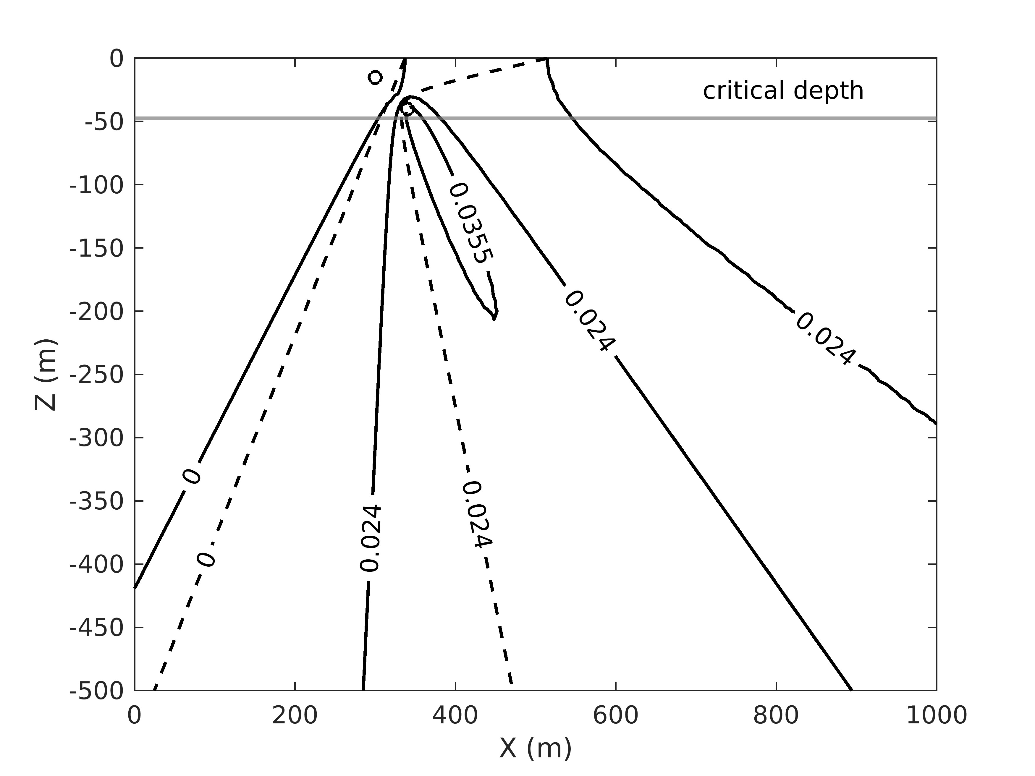
Figure 9: Contours of measured TDOA ($\delta t_{m}$) (s) from two receivers (circles) computed from dense grid of acoustic sources in Cartesian $(x,z)$ plane. Source emits exponential pulse (Eq. 32, $\tau=0.1$ s). $\delta t_{m}$ subject to interference between direct and reflected paths. In-situ speed of sound is 1500 m/s. Hyperbolas (dashed) compared with isodiachrons (solid lines) for same $\delta t_{m}$. Source cannot be located via hyperbolas when $|\delta t_{m}|$ exceeds propagation time of sound from first to second receiver but can be located with isodiachrons. Receivers above critical depth (gray line).

Next, consider deriving the locations of a source in a horizontal plane where the emitted sound is an exponential pulse with $\tau=0.1$ s (Eq. 32). When the in-situ speed of sound is 1500 m/s, the critical depth is 47.5 m. Two receivers are placed at Cartesian $(x,y,z)$ coordinates (0,0,-30) and (0,300,-30) m and source at (900,20,-30) m (Fig. 10). The measured TDOA is multiplied by 1500 m/s to yield a hyperbola. It does not contain the source’s location. The source is 27.3 m from the closest point on the hyperbola. For the same measured TDOA, the isodiachron passes through the source. When the constant sound speed field is replaced by measured sound speeds as a function of depth (Fig. 11), the measured TDOA is multiplied by 1500 m/s to yield a hyperbola whose closest approach to the source is 46.1 m (Fig. 10). The isodiachron passes through the source because it utilizes different speeds along the paths to each receiver. The receivers are above the critical depth of 47.6 m.

The receivers and source are moved from $z=-30$ to $-90$ m, all below the critical depths for both the constant and measured sound speed fields. For the constant speed case, the hyperbola misses the source by 105.7 m at closest approach (Fig. 10C). There are two isodiachrons for this case, one of which passes through the source’s location. The situation is similar when the measured field of sound speed is used (Fig. 10D). The source is missed by the hyperbola by 112.9 m, but intersected by one of the isodiachrons.

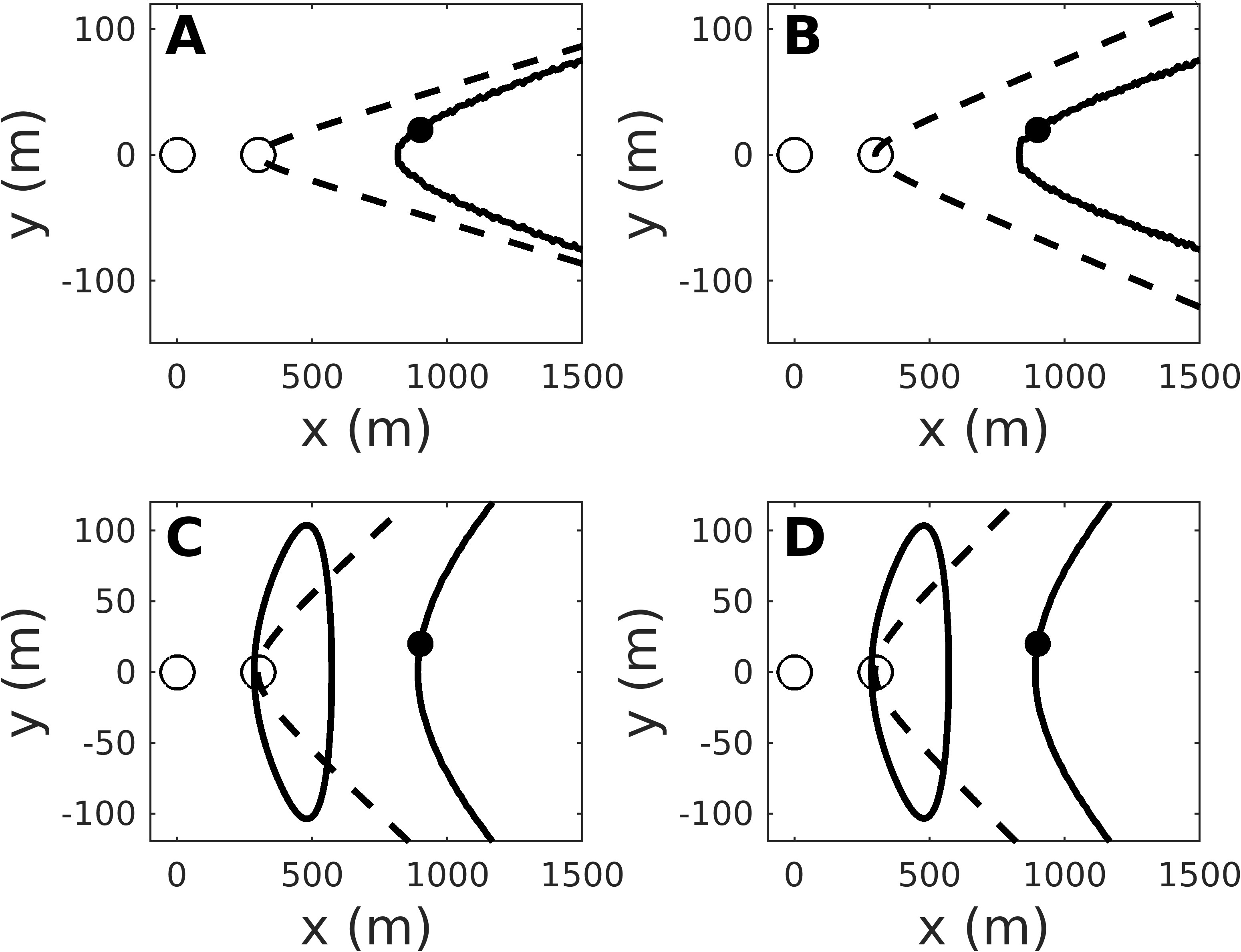
Figure 10: Hyperbola (dashed) and isodiachron (solid) for two receivers (open circles) and source (solid circle). A: Receivers above critical depth with in-situ sound speed of 1500 m/s. B: Same but sound speed derived from CTD data (Fig. 11). Receivers above critical depth. C: Same as A but receivers at 90 m depth. These are below critical depth. D: Same as C but sound speed derived from CTD data (Fig. 11)

.

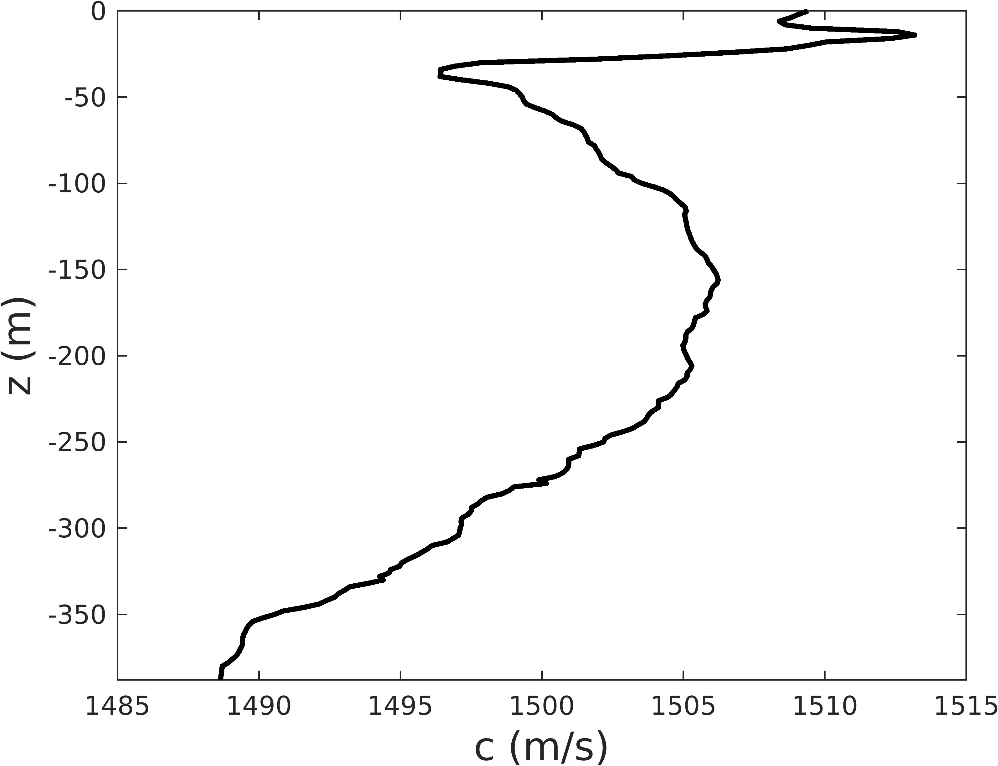
Figure 11: Sound speed (m/s) at different depths. Derived from measurements of conductivity, temperature, and depth at 17:09 30 May, 2022 Greenwich Mean Time at location 39.9608 $\mbox{}^{\circ}$N, 289.013 °E. Data courtesy Bill Hodgkiss, Scripps Institution of Oceanography.

V Discussion

Temporal interference between direct and reflecting paths can occur in solids, liquids, and gasses. This phenomenon potentially leads to large changes in the group speed of acoustic signals. In water, this speed often drops by orders of magnitude within hundreds of meters of a receiver and even approaches zero when the source and receiver are above the critical depth and near each other (Eq. 16). Many commonly-used methods for locating sounds require a single speed of sound as an input to convert a TDOA to a difference in distance from a pair of receivers, by which location is geometrically interpreted as lying on a hyperbola or hyperboloid [36, 35, 24, 11, 25, 69, 3]. However, when a source is near one receiver and distant from another, the group speeds to each receiver could be as different as 1 m/s and 1500 m/s. This implies hyperbolas are inappropriate for interpreting or deriving location. Previous results based on these models should be reconsidered when the source might be near at least one receiver.

The isodiachron is an appropriate geometrical interpretation of location derived with TDOA when the speeds of propagation differ between the source and each receiver [51]. This geometry was invented for the purpose of deriving reliable locations in these circumstances. Several illustrations of their efficacy here demonstrates the true location of the source lies on an isodiachron but not on a hyperbola where miss distances range from 10 to 100 m (Figs. 9,10). Apparently, reliable CIL need to account for the large decreases in group speed near the receivers. At least one method using isodiachrons is designed to generate reliable CIL in the presence of these variations of speed [53, 34].

The intricacy of generating reliable CIL near receivers seems unintuitive because the action is all occurring near the receivers where everything should seemingly be simple, but this is not so. A similar complexity was recently discovered for 2D models of location where the vertical coordinate is discarded and location is estimated with horizontal coordinates only. The 2D effective speed of sound used to derive location must vary with horizontal distance from the receiver if a correct location is desired [54]. This speed goes to zero meters per second when the source is above or below the receiver. This behavior is entirely caused by removing the vertical coordinate from the method of location. The requirement of zero speed above and below each receiver gave rise to the phrase, 2D black holes, to highlight their importance in 2D models for location [54]. A narrated tutorial of 2D black holes and isodiachrons is available in the supplementary material in [34]. In this paper, interference causes the group speed to decrease to zero meters per second in three-dimensional space near a receiver. This is a real physical phenomenon and not a consequence of eliminating a vertical coordinate when deriving location. In this sense, there are acoustical black holes near receivers in 3D space when interference occurs between the direct and reflected paths. This is an analogy to the naming of gravitational black holes where the speed of light goes to zero at the event horizon of a black hole. We now see there are both 2D and 3D acoustical black holes.

VI Author Declarations

Sequential bound estimation and its related technologies is a commercial location service. No other conflicts of interest.

The data that support the findings of this study are available within the article and its supplementary material.

References

- Bailey et al. [12] Bailey, H., Fandel, A. D., Silva, K., Gryzb, E., McDonald, E., Hoover, A. L., Ogburn, M. B., and Rice, A. N. (12). “Identifying and predicting occurrence and abundance of a vocal animal species based on individually specific calls,” Ecosphere 8.
- Bailey et al. [2019] Bailey, H., Rice, A., Wingfield, J. E., Hodge, K. B., Estabrook, B. J., Hawthorne, D., Garrod, A., Fandel, A. D., Fouda, L., McDonald, E., Grzyb, E., Fletcher, W., and Hoover, A. L. (2019). “Determining habitat use by marine mammals and ambient noise levels using passive acoustic monitoring offshore of Maryland,” OCS Study BOEM 2019-018.
- Baumgartner et al. [2008] Baumgartner, M., Freitag, L., Parta, J., Ball, K., and Prada, K. (2008). “Tracking large marine predators in three dimensions: the real-time acoustic tracking system,” IEEE J. Ocean Eng. 33, 146–157.
- Birchfield [2004] Birchfield, S. T. (2004). “A unifying framework for acoustic localization,” in 2004 12th European Signal Processing Conference, pp. 1127–1130.
- Birchfield and Gillmor [2002] Birchfield, S. T., and Gillmor, D. K. (2002). “Fast bayesian acoustic localization,” in 2002 IEEE International Conference on Acoustics, Speech, and Signal Processing, Vol. 2, pp. II–1793–II–1796.
- Brekhovskikh and Lysanov [1991] Brekhovskikh, L. M., and Lysanov, Y. P. (1991). Fundamentals of Ocean Acoustics (Springer-Verlag).
- Cato et al. [2019] Cato, D. H., Noad, M., and McCauley, R. (2019). “Understanding marine mammal presence in the Virginia offshore wind energy area,” OCS Study BOEM 2019-020.
- Clark et al. [2023] Clark, C. W., Charif, R. A., Hawthorne, D., Rahaman, A., Givens, G. H., George, J. C., and Muirhead, C. A. (2023). “Acoustic data from the spring 2011 bowhead whale census at Point Barrow, Alaska,” International Whaling Commission \dodoihttps://doi.org/10.47536/jcrm.v19i1.413.
- Clark et al. [1996] Clark, C. W., Charif, R. A., Mitchell, S. G., and Colby, J. (1996). “Distribution and behavior of the bowhead whale, Balaena mysticetus, based on analysis of acoustic data collected during the 1993 spring migration off point barrow, alaska,” Alaska. Sci. Rept., Intl. Whal. Commn. 46, 541–552.
- Clark et al. [2010] Clark, C. W., Ellison, W. T., Hatch, L. T., Merrick, R. L., Parijs, S. M. V., and Wiley, D. N. (2010). “An ocean observing system for large-scale monitoring and mapping of noise throughout the Stellwagen Bank National Marine Sanctuary,” Technical Report.
- Collier [2023] Collier, T. (2023). “Acoustic localization: Batch processing of wired-array data” https://github.com/travc/locbatch/, \dodoi10.1177/1045389X16667559.
- Collier et al. [2010] Collier, T. C., Kirschel, A. N., and Taylor, C. E. (2010). “Acoustic localization of antbirds in a mexican rainforest using a wireless sensor network,” J. Acoust. Soc. Am. 128, 182–189.
- Dunlop et al. [2008] Dunlop, R. A., Cato, D. H., and Noad, M. J. (2008). “Non-song acoustic communication in migrating humpback whales (Megaptera novaeangliae),” Marine Mammal Science 24(3), 613–629, \dodoi10.1111/j.1748-7692.2008.00208.x.
- Dunlop et al. [2014] Dunlop, R. A., Cato, D. H., and Noad, M. J. (2014). “Evidence of a Lombard response in migrating humpback whales (Megaptera novaeangliae),” J. Acoust. Soc. Am. 136(1), 430–437, \dodoi10.1121/1.4883598.
- Dunlop et al. [2013a] Dunlop, R. A., Cato, D. H., Noad, M. J., and M., D. (2013a). “Source levels of social sounds in migrating humpback whales (Megaptera novaeangliae),” J. Acoust. Soc. Am. 134, 706–714.
- Dunlop et al. [2013b] Dunlop, R. A., Cato, D. H., Noad, M. J., and Stokes, D. M. (2013b). “Source levels of social sounds in migrating humpback whales (Megaptera novaeangliae),” J. Acoust. Soc. Am. 134(1), 706–714, \dodoi10.1121/1.4807828.
- Dunlop et al. [2013c] Dunlop, R. A., Noad, M. J., Cato, D. H., Kniest, E., Miller, P. J. O., Smith, J. N., and Stokes, M. D. (2013c). “Multivariate analysis of behavioural response experiments in humpback whales (Megaptera novaeangliae),” J. Experimental Biology 216(5), 759–770, \dodoi10.1242/jeb.071498.
- Dunlop et al. [2007] Dunlop, R. A., Noad, M. J., Cato, D. H., and Stokes, D. (2007). “The social vocalization repertoire of east Australian migrating humpback whales (Megaptera novae angliae),” J. Acoust. Soc. Am. 122(5), 2893–2905, https://doi.org/10.1121/1.2783115, \dodoi10.1121/1.2783115.
- Dunlop et al. [2015] Dunlop, R. A., Noad, Michael J., M. R. D., Kneist, E., Paton, D., and Cato, D. H. (2015). “The behavioural response of Humpback whales (textitMegaptera novaeangliae) to a 20 cubic inch air gun.,” Aquatic Mammals 41(4), 412–433, \dodoi10.1578/AM.41.4.2015.412.
- Fandel et al. [2022] Fandel, A., Hodge, K., Rice, A., and Bailey, H. (2022). “Altered spatial distribution of a marine top predator under elevated ambient sound conditions,” in State of the Science Workshop on Wildlife and Offshore Wind Energy 2022, New York State Energy Research and Development Authority.
- Fermat [1891] Fermat, A. C. (1891). Oeuvres de Fermat (Paris: Gauthier-Villars et fils).
- Feynman [1985] Feynman, R. P. (1985). QED. The strange theory of light and matter (Princeton University Press).
- Feynman et al. [2011] Feynman, R. P., Leighton, R. B., and Sands, M. L. (2011). The Feynman lectures on physics (New millennium ed, New York).
- Gillespie et al. [2008] Gillespie, D., Gordon, J., McHugh, R., McLaren, D., Mellinger, D. K., Redmond, P., T. A., Trinder, P., and Deng, X. Y. (2008). “PAMGUARD: Semiautomated, open source software for real-time acoustic detection and localisation of cetaceans,” Proc. Inst. Acoust. 30, 9 pp.
- Greene et al. [2016] Greene, E., Shiu, Y., Morano, J., Clark, C., Little, P., Billings, A., and Hawthrone, D. (2016). “A practical guide for designing recording arrays in terrestrial environments: Best practices for maximizing location accuracy and precision,” in Ecoacoustics Congress 2016, International Society of Ecoacoustics (ISE).
- Hau et al. [1999] Hau, L. V., Harris, S. E., Dutton, Z., and Behroozi, C. H. (1999). “Light speed reduction to 17 meters per second in an ultracold atomic gas,” Nature 397, 594–598.
- Helstrom [1975] Helstrom, C. W. (1975). Statistical Theory of Signal Detection (Pergamon).
- Hoeck et al. [2023] Hoeck, R. V. V., Rowell, T. J., Dean, M. J., Rice, A. N., and Parijs, S. M. V. (2023). “Comparing atlantic cod temporal spawning dynamics across a biogeographic boundary: Insights from passive acoustic monitoring,” Technical Report, \dodoihttps://doi.org/10.1002/mcf2.10226.
- [29] john.spiesberger@gmail.com. “Scientific innovations, inc.” .
- Levenberg [1944] Levenberg, K. (1944). “A method for the solution of certain non-linear problems in least squares,” Quart. Appl. Math 2, 164–168.
- Liu et al. [2001] Liu, C., Dutton, Z., Behroozi, C. H., and Hau, L. V. (2001). “Observation of coherent optical innformation storage in an atommic medium using halted light pulses,” Nature 409, 594–598.
- Lloyd [1831] Lloyd, H. (1831). “On a new case of interference of the rays of light,” The Transactions of the Royal Irish Academy 17, 171–177.
- Marquardt [1963] Marquardt, D. (1963). “An algorithm for least-squares estimation of nonlinear parameters,” SIAM J. Appl. Math. 11, 431–441.
- Mathur et al. [2024] Mathur, M., Spiesberger, J., and Pascoe, D. (2024). “Confidence intervals of location for marine mammal calls via time-differences-of-arrival: Sensitivity analysis,” JASA Express Lett. 4.
- Mellinger [2024] Mellinger, D. (2024). “Osprey: sound visualization, measurement, localization” https://www.mathworks.com/matlabcentral/fileexchange/166186-osprey-sound-visualization-measurement-localization.
- Mellinger [2001] Mellinger, D. K. (2001). “Ishmael 1.0 user’s guide,” NOAA Technical memorandum OAR PMEL-120, available from NOAA/PMEL/OERD, 2115 SE OSU Drive, Newport, OR 97365-525.
- Mennill et al. [2006] Mennill, D. J., Burt, J. M., Fristrup, K. M., and Vehrencamp, S. L. (2006). “Accuracy of an acoustic location system for monitoring the position of duetting songbirds in tropical forest,” J. Acoust. Soc. Am 119, 283202839.
- Merriam-Webster [2023] Merriam-Webster (2023). “hyperbola” https://www.merriam-webster.com/dictionary/hyperbola.
- Milne [1886] Milne, J. (1886). Earthquakes and other Earth movements (D. Appleton and Co., New York).
- Mitchell and Bower [1995] Mitchell, S., and Bower, J. (1995). “Localization of animal calls via hyperbolic methods,” J. Acoust. Soc. Am. 97, 3352–3353.
- Moré et al. [1980] Moré, J. J., Garbow, B. S., and Hillstrom, K. E. (1980). “User Guide for MINIPACK-1,” Argonne National Laboratory Report ANL-80-74.
- Muanke and Niezrecki [2007] Muanke, P. B., and Niezrecki, C. (2007). “Manatee position estimation by passive acoustic localization,” J. Acoust. Soc. Am. 121(4), 2049–2059, https://doi.org/10.1121/1.2532210, \dodoi10.1121/1.2532210.
- Murray [2015] Murray, A. (2015). “The simple and complex phrase types of humpback wahle (Megaptera novaeangliae) song,” Ph.D. dissertation, The University of Queensland, Brisbane, AU.
- of Defense [2011] of Defense, D. (2011). “Technology readiness levels” https://www.ncbi.nlm.nih.gov/books/NBK201356/.
- Review [2018] Review, T. I. H. (2018). ““determination of velocity of sound in seawater in cape cod bay,” The International Hydrographic Review .
- Risch et al. [2014] Risch, D., Siebert, U., and Parijs, S. M. V. (2014). “Individual calling behaviour and movements of north atlantic minke whales (balaenoptera acutorostrata),” Brill 151.
- Salisbury et al. [2018] Salisbury, D. P., Estabrook, B. J., Klinck, H., and Rice, A. N. (2018). “Understanding marine mammal presence in the Virginia offshore wind energy area,” OCS Study BOEM 2019-007.
- Schmidt [1972] Schmidt, R. O. (1972). “A new approach to geometry of range difference location,” IEEE Trans. on Aerospace and Elect. Sys. AES-8, 821–835.
- Special prohibitions for endangered marine mammals [2023] Special prohibitions for endangered marine mammals (2023). “50 cfr 224.103” https://www.ecfr.gov/current/title-50/chapter-II/subchapter-C/part-224/section-224.103.
- Spiesberger [15] Spiesberger, J. (15). “Estimation algorithms and location techniques” U.S. patent 7,219,032.
- Spiesberger [2004] Spiesberger, J. (2004). “Geometry of locating sounds from differences in travel time: isodiachrons,” J. Acoust. Soc. Am 116(5), 3168–3167.
- Spiesberger [2005a] Spiesberger, J. (2005a). “Probability distributions for locations of calling animals, receivers, sound speeds, winds, and data from travel time differences,” J. Acoust. Soc. Am. 118, 1790–1800.
- Spiesberger [2005b] Spiesberger, J. (2005b). “Probability distributions for locations of calling animals, receivers, sound speeds, winds, and data from travel time differences,” J. Acoust. Soc. Am 118, 1790–1800.
- Spiesberger [2020] Spiesberger, J. (2020). “Dimension reduction in location estimation - the need for variable propagation speed,” Acoustical Physics 66, 178–190.
- Spiesberger et al. [2021] Spiesberger, J., Berchok, C., Iyer, P., Schoeny, A., Sivakumar, K., Woodrich, D., Yang, E., and Zhu, S. (2021). “Bounding the number of calling animals with passive acoustics and reliable locations,” J. Acoust. Soc. Am 150(10.1121/10.0004994), 1496–1504.
- Spiesberger and Fristrup [1990] Spiesberger, J., and Fristrup, K. (1990). “Passive localization of calling animals and sensing of their acoustic environment using acoustic tomography,” The American Naturalist 135, 107–153.
- Spiesberger et al. [2022] Spiesberger, J., Garcia, M., Klinck, H., and Shiu, Y. (2022). “Extremely-reliable locations and calling abundance or right whales in Cape Cod Bay derived with passive recordings of their calls with un-synchronized clocks,” in Detection, Classification, Localization, and Estimation, Oahu, Vol. 1, p. 24, https://www.soest.hawaii.edu/ore/dclde/wp-content/uploads/2022/03/DCLDE-2022-Abstracts.pdf.
- Spiesberger and Wahlberg [2002] Spiesberger, J., and Wahlberg, M. (2002). “Probability density functions for hyperbolic and isodiachronic location,” J. Acoust. Soc. Am. 112, 3046–3052.
- Spiesberger [2001] Spiesberger, J. L. (2001). “Hyperbolic location errors due to insufficient number of receivers,” J. Acoust. Soc. Am. 109, 3076–3079.
- Spiesberger [2008] Spiesberger, J. L. (2008). “Estimation methods for wave speed” U.S. Patent No. 7,363,191.
- Spiesberger [2011] Spiesberger, J. L. (2011). “Methods for estimating location using signal with varying signal speed” U.S. Patent No. 8,010,314.
- Spiesberger [2012] Spiesberger, J. L. (2012). “Methods and apparatus for computer-estimating a function of a probability distribution of a variable” U.S. Patent No. 8,311,773.
- Spiesberger [2014] Spiesberger, J. L. (2014). “Methods and computerized machine for sequential bound estimation of target parameters in time-series data” U. S. Patent No. 8639469.
- Spiesberger [2017] Spiesberger, J. L. (2017). “Final report, target localization using muti-static sonar with drifting sonobuoys” Contract N68335-12-C-000211.
- Spiesberger [2021] Spiesberger, J. L. (2021). “Estimation of clock synchronization errors using time difference of arrival” US patent 10915137.
- Spiesberger [2023] Spiesberger, J. L. (2023). “Estimation of clock synchronization errors using time difference of arrival” CA 3107173.
- Stanistreet et al. [2013] Stanistreet, J. E., Risch, D., and Parijs, S. M. V. (2013). “Passive acoustic tracking of singing humpback whales (Megaptera novaeangliae) on a Northwest Atlantic feeding ground,” Plos One \dodoihttps://doi.org/10.1371/journal.pone.0061263.
- [68] Statek Corporation. “Cs-1v-sm crystal oscillator” .
- Urazghildiiev and Clark [2013] Urazghildiiev, I. R., and Clark, C. W. (2013). “Comparative analysis of localization algorithms with application to passive acoustic monitoring,” J. Acoust. Soc. Am 134(6), \dodoi10.1121/1.4824683.
- Wiggins [2003] Wiggins, S. (2003). “Autonomous acoustic recording packages (arps) for long-term monitoring of whale sounds,” Marine Technology Society Journal 37(2), 13–22, \dodoi10.4031/002533203787537375.
- Wiggins et al. [2013] Wiggins, S. M., Frasier, K. E., Elizabeth Henderson, E., and Hildebrand, J. A. (2013). “Tracking dolphin whistles using an autonomous acoustic recorder array,” J. Acoust. Soc. Am. 133(6), 3813–3818, \dodoi10.1121/1.4802645.