No Pulsar Timing Noise from Brownian Motion of the Sun

Abstract

It was recently claimed [Loeb (2024a)] that evidence for a stochastic gravitational wave background observed by pulsar timing arrays can be attributed instead to random perturbations of the Sun’s motion by transiting asteroids. I show that that this would lead to a large dipole component accompanying a much smaller quadrupolar perturbation of pulsar timing signals, which would not be confused with a gravitational wave signal. Such an anomalous dipole would have been detected and identified as a spurious background by the PTA collaborations, if it existed.

Loeb (2024a) recently argued that the stochastic gravitational wave signal observed by pulsar timing arrays could be explained by perturbations in the Sun’s motion, caused by an unmodeled population of asteroids. This anomalous motion would produce a Doppler distortion of the pulsar arrival times, with the same magnitude (at least until Loeb (2024b); 20% of the observed signal subsequently) and frequency as the purported gravitational waves.

Starting in arXiv version 4, Loeb (2024a) recognized that the predicted distortion should be dipolar, whereas the GW signal must be quadrupolar, but minimized this distinction by saying “it is challenging to separate the 3D random walk of a dipole sourced by a torodial configuration of asteroids around the Sun from a quadrupolar random walk sourced by a stochastic gravitational wave background, given the small number of independent correlation times ($\sim 5$ periods of $\sim 3$ years) available during the 15 years of PTA observations.”

We believe this argument is incorrect. Consider two pulsars with whose directions on the sky relative to Earth are described by the unit vectors $\hat{k}_{1}$ and $\hat{k}_{2}$, such that $\hat{k}_{1}\cdot\hat{k}_{2}=\cos\theta$. Suppose that there are five sequential asteroids that perturb the Earth’s velocity by $\vec{v}_{i}$ for $i=1,5$. The signal from a given pulsar $p$ while the Earth is perturbed by asteroid $a$ is proportional to $\cos([\omega_{p}-\vec{v}_{a}\cdot\hat{k}_{p}/c]t+\phi_{p})$. The fractional perturbation of the pulsar frequency is given by

$${\delta\omega_{p,a}\over\omega_{p,a}}={\vec{v}_{a}\cdot\hat{k}_{p}\over c}\,.$$ (1)

Since these residuals become stacked during the multiyear observation period, we are interested in $\delta_{p}=\sum_{a}\delta\omega_{p,a}/\omega_{p,a}\equiv\hat{k}_{p}\cdot\vec{V}$. Depending on details of the asteroid transit, this sum might be weighted by dimensionless factors $b_{a}$ so that $\vec{V}=(1/c)\sum_{a}b_{a}\vec{v}_{a}$. $\vec{V}$ represents the effective mean velocity perturbation to the Earth during the observing period, in units of $c$. In Loeb (2024c) it was estimated that $v_{a}\sim 3\times 10^{-5}$ cm/s, corresponding to an amplitude $V\sim 10^{-15}$.

Now consider the correlation between timing residuals, $\langle\delta_{1}\,\delta_{2}\rangle$, averaged over all pulsars having similar angular separation $\sim\theta$. For $N$ pulsars, this is given by

$$\langle\delta_{1}\,\delta_{2}\rangle_{\theta} = {2\over N(N-1)}\sum_{p^{\prime}<p}{\hat{k}_{p}\cdot\vec{V}}\,{\hat{k}_{p}\cdot\vec{V}}$$ (2)

$$\times W(\hat{k}_{p}\cdot\hat{k}_{p^{\prime}}-\cos\theta)$$

where $W$ is a window function with support in the angular bin containing $\theta$. In the limit $N\to\infty$ with pulsars uniformly distributed over the sky, it is straightforward to show that $\langle\delta_{1}\,\delta_{2}\rangle_{\theta}\propto\cos\theta$, a purely dipolar distribution. For finite $N$, we expect fluctuations that can randomly produce a small quadrupole component.

To quantify this, we have simulated the signal that could be expected for the NANOGrav pulsar timing array [Agazie et al. (2024)], which contains $N=68$ pulsars with positions on the sky that are identified by their names (right ascension and declination). Using the same 15 angular bins (each containing $\sim 150$ pulsar pairs) adopted by NANOGrav, the resulting angular correlations are shown for random choices of the velocity perturbation orientation $\vec{V}$ in Fig. 1. We fit the results to a linear combination of Legendre polynomials $a_{1}P_{1}+a_{2}P_{2}$, allowing for a dipole plus quadrupole component, and show the ratio $a_{2}/a_{1}$. For velocity perturbations with no restriction on orientation, the average is $\langle a_{2}/a_{1}\rangle=0.16$, while for $\vec{V}$ restricted to vanishing declination, as a simplified model for asteroids lying roughly in the ecliptic plane, the average is $0.05$.

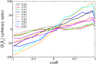
Figure 1: Angular correlation function of pulsar timing frequency residuals for random choices of the velocity perturbation $\vec{V}$. Left: $\vec{V}$ is allowed to vary over $4\pi$. Right: $\vec{V}$ is restricted to the plane of declination zero, roughly aligned with the ecliptic. Legend shows relative contribution of quadrupole versus dipole in best fit.

According to Loeb (2024c), as much as 20% of the NANOGrav GW signal could be mimicked by this source of noise; in this case, an accompanying dipolar contamination of intensity $0.2/0.16\sim 1$ times the quadrupolar signal should have been observed. The PTA collaborations carefully account for peculiar motion of the Earth in order to remove such backgrounds; hence any unmodeled source strong enough to affect the inferred gravitational wave signal would have stood out in the data as an anomalous dipole contribution [Caballero et al. (2018); Li et al. (2016); Champion et al. (2010)]. The Bayseian odds against the dipole interpretation were found to be $10^{7}$ in Agazie et al. (2023), contradicting the claim of Loeb (2024c) by many orders of magnitude. Fig. 7 of the NANOGrav discovery paper [Agazie et al. (2023)] shows a subdominant contamination of the quadrupole signal by a dipole component at the level of $a_{1}/a_{2}=\sqrt{0.2/1.8}\sim 0.3$, opposite to the behavior in Fig. 1, which predicts $a_{1}/a_{2}>6$. Therefore even a 20% contribution to the inferred GW signal from anomalous motion of the sun is strongly contradicted by the PTA analysis.

Acknowledgment. I thank Valerie Domcke, Boris Goncharov and Matthew McCullough for helpful discussions.

References

- Agazie et al. (2023) Agazie, G., et al. 2023, Astrophys. J. Lett., 951, L8, doi: 10.3847/2041-8213/acdac6
- Agazie et al. (2024) —. 2024, Astrophys. J. Lett., 964, L14, doi: 10.3847/2041-8213/ad2a51
- Caballero et al. (2018) Caballero, R. N., et al. 2018, Mon. Not. Roy. Astron. Soc., 481, 5501, doi: 10.1093/mnras/sty2632
- Champion et al. (2010) Champion, D. J., et al. 2010, Astrophys. J. Lett., 720, L201, doi: 10.1088/2041-8205/720/2/L201
- Li et al. (2016) Li, L., Guo, L., & Wang, G.-L. 2016, Research in Astronomy and Astrophysics, 16, 006, doi: 10.1088/1674-4527/16/4/058
- Loeb (2024a) Loeb, A. 2024a. https://arxiv.org/abs/2405.05410v4
- Loeb (2024b) —. 2024b. https://arxiv.org/abs/2405.05410v6
- Loeb (2024c) —. 2024c, Astrophys. J. Lett., 968, L27, doi: 10.3847/2041-8213/ad53c9