Efficient Measurement-Driven Eigenenergy Estimation with Classical Shadows

Abstract

Quantum algorithms exploiting real-time evolution under a target Hamiltonian have demonstrated remarkable efficiency in extracting key spectral information. However, the broader potential of these methods, particularly beyond ground state calculations, is underexplored. In this work, we introduce the framework of multi-observable dynamic mode decomposition (MODMD), which combines the observable dynamic mode decomposition, a measurement-driven eigensolver tailored for near-term implementation, with classical shadow tomography. MODMD leverages random scrambling in the classical shadow technique to construct, with exponentially reduced resource requirements, a signal subspace that encodes rich spectral information. Notably, we replace typical Hadamard-test circuits with a protocol designed to predict low-rank observables, thus marking a new application of classical shadow tomography for predicting many low-rank observables. We establish theoretical guarantees on the spectral approximation from MODMD, taking into account distinct sources of error. In the ideal case, we prove that the spectral error scales as $\exp(-\Delta Et_{\rm max})$, where $\Delta E$ is the Hamiltonian spectral gap and $t_{\rm max}$ is the maximal simulation time. This analysis provides a rigorous justification of the rapid convergence observed across simulations. To demonstrate the utility of our framework, we consider its application to fundamental tasks, such as determining the low-lying, i.e. ground or excited, energies of representative many-body systems. Our work paves the path for efficient designs of measurement-driven algorithms on near-term and early fault-tolerant quantum devices.

I Introduction

Quantum algorithms based on real-time evolution [1, 2, 3, 4, 5, 6, 7, 8, 9, 10, 11, 12, 13, 14] have gained increasing popularity due to the unitarity of real-time dynamics and their native implementation on quantum hardware. In particular, real-time eigensolvers have demonstrated impressive efficacy in extracting the ground state information of physical many-body systems. This success raises a natural question: can the algorithms perform highly accurate excited state calculations?

The real-time approaches were initially conceptualized from a subspace diagonalization perspective [1, 2]. While, in theory, these subspace methods have the potential to uncover spectral information beyond the ground state, they typically involve solving ill-conditioned generalized eigenvalue problems [15] and can thus suffer from perturbative errors, including standard hardware noise. Alternatively, recent approaches [7, 16, 8, 10, 11] draw inspirations from a signal processing perspective, where real-time evolution is primarily utilized to generate time series that resonate with the target eigenmodes. In general, the signal processing approaches are resilient to perturbative noise due to their robust regularization. On the other hand, they often rely on state preparation such that the initial state undergoing the Hamiltonian dynamics should overlap dominantly with the eigenstates of interest. Without such a basic assumption, accurately finding multiple eigenenergies may demand substantial quantum or classical resources.

In this work, we introduce a real-time evolution framework that flexibly combines real-time quantum evolution with classical data post-processing to access both ground and lower excited state energies of a quantum many-body system. Specifically, our framework is efficient as it only requires the preparation of a single, simple initial state on the quantum computer, with overall resource demands comparable to the leading ground state algorithms. Furthermore, our classical post-processing is ansatz-free and completely circumvents the challenges of complex optimization landscapes commonly encountered in parametric methods, particularly as the number of target eigenenergies increases [17, 18, 19].

The main technical tools that we leverage are classical shadow tomography [20, 21, 22, 23, 24, 25, 26] and observable dynamic mode decomposition (ODMD) [9]. We develop a simple, single-ancilla shadow protocol to collect real-time signals associated with many observables, and utilize ODMD to unravel these signals into single-energy modes. Since oscillating time signals with distinct power spectra are linearly independent in the space of all sinusoidal functions, they form the basis of some signal subspace, which can be systematically expanded to accommodate the desired frequencies. Our approach, termed the multi-observable dynamic mode decomposition (MODMD), can hence be viewed as a unifying framework that enjoys the strength of both subspace and signal processing algorithms.

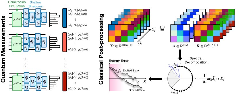
Figure 1: MODMD for eigenenergy estimation. MODMD collects the expectations, ${\rm Tr}\left[\rho(k\Delta t)\Gamma_{O}\right]=\Re\bra{\phi_{0}}Oe^{-iHk\Delta t}\ket{\phi_{0}}$, with respect to a simple reference state $\ket{\phi_{0}}$. This data can be measured efficiently on a quantum processor through Hamiltonian simulations combined with shadow tomographic techniques, where the shadow circuits can be shallow with a depth logarithmic in the number of qubits. MODMD then constructs a pair of block Hankel matrices $(\mathbf{X},\mathbf{X}^{\prime})$, and computes the DMD system matrix $A$ that adopts a block companion structure. The eigenvalues $\tilde{\lambda}_{n}$ of $A$ converge to the true eigenphases $\lambda_{n}$ as the size of $\mathbf{X}$ and $\mathbf{X}^{\prime}$ increases. The low-lying energies $E_{n}$ are estimated as angles of $\tilde{\lambda}_{n}$, $\tilde{E}_{n}=-\frac{1}{\Delta t}\text{arg}(\tilde{\lambda}_{n})$.

Compared to alternative hybrid eigensolvers, our real-time framework has the following notable advantages: it (1) achieves near-exponential convergence of the eigenenergy estimates surpassing the conventional Fourier limit, (2) provides extensive knowledge of a many-body system including eigenstate properties and dynamical responses, and (3) significantly saves quantum resources in terms of the evolution time while showing stability against perturbative noise. These features make our algorithm promising for near-term implementations on current quantum platforms, such as analog quantum simulators and early fault-tolerant quantum computers.

The manuscript is organized as follows. In Section II, we first overview key concepts underlying recent advances in real-time eigensolvers. We then establish in Section III the building blocks of real-time MODMD framework and detail our core algorithm for eigenenergy and eigenstate estimation. Theoretical guarantees on its convergence and preliminary error analysis are presented within Section IV. Finally, we numerically demonstrate our algorithm in Section V by focusing on many-body examples from condensed matter physics and quantum chemistry.

II Preliminaries

In this work, we develop an approach that gives highly accurate eigenenergy estimates beyond the ground state. Specifically, we propose a real-time framework combining the observable dynamic mode decomposition (ODMD) and classical shadow tomography, where we fully leverage the synergy between these two algorithmic components. We will show that we can design a simple shadow protocol to predict the real-time expectation value $\braket{\phi_{0}}{Oe^{-iHt}}{\phi_{0}}$ for the problem Hamiltonian $H$ and a reference state $\ket{\phi_{0}}$. In particular, classical shadows enable the simultaneous prediction of expectations for many observables $O$ of our choice. These expectations generate a multivariate time series, whose characteristic frequencies can be efficiently extracted by ODMD.

From here on, we will use $\mathcal{H}\subset\mathbb{C}^{N}$ to denote the physical Hilbert space of many-body quantum states and $\mathbb{L}(\mathcal{H})$ to denote the Liouville space, i.e., the space of linear operators acting on $\mathcal{H}$ (we work with finite-dimensional and thus bounded linear operators for simplicity). Additional essential notations are defined self-consistently in Table 1 and throughout the main text.

II.1 Real-time quantum eigensolvers

In this subsection, we first highlight the capabilities of real-time evolution in determining the eigenenergies of a target Hamiltonian $H\in\mathbb{C}^{N\times N}$. We consider the spectral decomposition, $H=\sum_{n=0}^{N-1}E_{n}\ket{\psi_{n}}\bra{\psi_{n}}$, of the Hamiltonian with ordered energies $E_{0}\leq E_{1}\leq\ldots\leq E_{N-1}$. The real-time approaches commonly require evaluation of the expectation value [1, 2, 3, 5, 7, 16, 8, 9, 10, 11, 12, 13],

$$\braket{\phi_{0}}{e^{-iHt}}{\phi_{0}}=\sum_{n=0}^{N-1}\mathinner{\!\left\lvert\alpha_{n}\right\rvert}^{2}e^{-iE_{n}t},$$ (1)

where $\ket{\phi_{0}}\in\mathcal{H}$ is a reference state, $\alpha_{n}=\braket{\psi_{n}}{\phi_{0}}$ is the overlap between the reference state and eigenstate $\ket{\psi_{n}}$, and $t=k\Delta t$ is typically an integer multiple of some time step $\Delta t$. The expectation can be efficiently sampled from repeated quantum measurements through the Hadamard test [27] or mirror fidelity estimation [28, 5].

There are several approaches for obtaining energy estimates from data of the type Eq. 1. Quantum subspace diagonalization [1, 2, 3, 5, 13, 12] variationally approximates the extremal eigenenergies by forming a projected eigenvalue problem, where a subspace can be built through successive real-time evolutions as new matrix elements with increasing $k$ are added. In essence, the subspace methods construct some polynomial $p(\lambda_{n})$ evaluated at the eigenphases $\lambda_{n}=e^{-iE_{n}\Delta t}$, where the degree of the polynomial $p$ precisely matches the number of time steps; an accurate ground state estimation then demands $|p(\lambda_{0})|\gg|p(\lambda_{n})|\approx 0$ for $n>0$. With a single reference state $\ket{\phi_{0}}$, these methods often struggle to locate excited states, though convergence can be potentially accelerated by the preparation of multiple reference states with a cost quadratic in their number. Moreover, we notice that the real-time states $\{e^{-iHk\Delta t}\ket{\phi_{0}}\}_{k\geq 0}$ lose orthogonality as a subspace basis, which can thereby lead to ill-conditioning and susceptibility to noise.

Table 1: Glossary of key notations.

Hilbert space	$\mathcal{H},~{}{\rm dim}\mathcal{H}=N=2^{L}$
Liouville space	$\mathbb{L}(\mathcal{H}),~{}{\rm dim}\mathbb{L}(\mathcal{H})=N^{2}$
Hamiltonian in Pauli basis	$H=\sum_{\nu=1}^{M}\kappa_{\nu}P_{\nu}$
Hermitian observables	$O_{i}=\sum_{\nu=1}^{M_{i}}\kappa_{i,\nu}P_{i,\nu}$
Pure quantum state	$\rho_{\phi}=\ket{\phi}\bra{\phi}$
Multi-observable signal	$\{\braket{\phi_{0}}{O_{i}e^{-iHt}}{\phi_{0}}\}_{i=1}^{I}$
Classical shadow dataset	$\{\hat{\sigma}_{q}=U_{q}^{\dagger}|b_{q}\rangle\langle b_{q}|U_{q}\}_{q=1}^{Q}$
Systematic error (e.g., shot noise)	$\epsilon_{1}$
Algorithmic error from eigensolver	$\epsilon$

Alternatively, the signal processing methods [7, 8, 16, 11, 10] capitalize on Fourier or harmonic analysis to resolve the eigenfrequencies or eigenenergies of interest. These methods mitigate the impact of noise by minimizing a customized objective function, which sharpens into robust optima as the number of time steps increases. Despite the resilience to noise, the optimization landscape depends critically on the choice of the reference state $\ket{\phi_{0}}$. For example, let us consider Eq. 1 as a spectral density over the unit circle, where the squared overlap $\lvert\alpha_{n}\rvert^{2}$ indicates the normalized spectral weight. Techniques such as peak finding on the spectral density may not yield a unique solution when the reference state has nearly uniform eigenstate overlaps. To ensure accurate energy estimations, more sophisticated reference state preparations and post-processing designs need to be accounted for.

To access both ground and excited state properties, we aim for a simple, accurate, and robust real-time protocol. To this end, we will introduce a quantum signal subspace approach that utilizes signals of the form $\braket{\phi_{0}}{Oe^{-iHt}}{\phi_{0}}$ for general operators $O$. Importantly, we seek to measure many such operator expectations simultaneously with a cost logarithmic in the number of observables. This can be precisely achieved via classical shadows, which we explore in the following subsection.

Real-time methods	Measurement cost	Post-processing cost	Algorithmic convergence	Target overlap
Single-observable signal
Subspace [1, 2, 3, 5, 13, 12]	$\displaystyle\mathcal{O}\big{(}\epsilon_{1}^{-2}\big{)}$	poly($N_{\rm eig}$)	$\tilde{\mathcal{O}}(\epsilon_{1}^{-2})$ in low-$\epsilon_{1}$ limit	non-vanishing
			unstable in high-$\epsilon_{1}$ limit
Signal processing [7, 8, 11, 10]	$\displaystyle\mathcal{O}\big{(}\epsilon_{1}^{-2}\big{)}$	$\exp(N_{\rm eig})$ in some cases	$\displaystyle\tilde{\mathcal{O}}\big{(}\epsilon^{-1}\big{)}$	dominant
Multi-observable signal
Shadow spectroscopy [29]	$\displaystyle\mathcal{O}\big{(}\log(I)3^{{\rm loc}[O]}\epsilon_{1}^{-2}\big{)}$	poly$(N_{\rm eig})$	uncertain	non-vanishing
Signal subspace (this work)	$\displaystyle\mathcal{O}\big{(}\log(I)\epsilon_{1}^{-2}\big{)}$	poly$(N_{\rm eig})$	$\tilde{\mathcal{O}}\big{(}\epsilon^{-1}\big{)}$ in some cases	non-vanishing
			stable with respect to $\epsilon_{1}$ [30, 31]

Table 2: Landscape of real-time hybrid eigensolver leveraging quantum measurements of $\braket{\phi_{0}}{Oe^{-iHt}}{\phi_{0}}$ and classical post-processing schemes. We consider estimating a target set of Hamiltonian eigenergies, $\{E_{n}\mathrel{\mathop{\mathchar 58\relax}}n\in\mathcal{N}_{\rm eig}\subset[N]\}$, where $\lvert\mathcal{N}_{\rm eig}\rvert=N_{\rm eig}$ for $N_{\rm eig}\ll N$. On quantum hardware, real-time evolution of a reference state $\ket{\phi_{0}}$ is performed and different expectation values are measured with an uncertainty of $\epsilon_{1}$. The classical post-processing then extracts from these measurements our eigenenergy estimates with an algorithmic error of $\epsilon$.

II.2 Efficient measurement with classical shadows

Classical shadow tomography [20, 21, 32, 33, 34] embodies a powerful suite for efficiently measuring expectations of many observables simultaneously:

$${\rm Tr}\left[\rho_{\phi}\Gamma_{i}\right]=\braket{\phi}{\Gamma_{i}}{\phi},\qquad\{\Gamma_{i}\}_{i=1}^{I},$$ (2)

where $\Gamma_{i}\in\mathbb{L}(\mathcal{H})$ has an efficient representation on a classical computer. Here $\rho_{\phi}=\ket{\phi}\bra{\phi}\in\mathbb{L}(\mathcal{H})$ is a pure state, though a similar trace evaluation applies to mixed states. Classical shadow tomography consists of two key steps: (1) random quench evolution using $U\in\mathcal{U}$ from a unitary ensemble $\mathcal{U}$, and (2) computational basis measurement. Upon each measurement, the quantum state collapses to a bitstring $|b_{q}\rangle$. After repetitive experiments, one obtains a classical shadow dataset, $\{U_{q}^{\dagger}|b_{q}\rangle\langle b_{q}|U_{q}\}_{q=1}^{Q}$, which can be viewed as a classical sketch of the quantum state. It is known [20] that $Q=\mathcal{O}(\log(I)\max_{i}\mathinner{\!\left\lVert\Gamma_{i}\right\rVert}_{\text{sh}}\epsilon_{1}^{-2})$ shadows can predict all the $I$ expectation values given by Eq. 2 to uncertainty $\epsilon_{1}$ with high probability. Here, the shadow norm, $\mathinner{\!\left\lVert\Gamma\right\rVert}_{\text{sh}}$, depends on both the unitary ensemble $\mathcal{U}$ and the operator $\Gamma$. For example, when the ensemble $\mathcal{U}$ is the $L$-qubit random Clifford unitaries, i.e., $\mathcal{U}=\text{Cl}(2^{L})$, and the operator $\Gamma=\Gamma^{\dagger}$ is Hermitian, the shadow norm is $\mathinner{\!\left\lVert\Gamma\right\rVert}_{\text{sh}}=3{\rm Tr}[\Gamma^{2}]$. This is especially powerful if $\Gamma$ is low-rank, meaning that its operator rank stays independent of the system size. Because ${\rm Tr}[\Gamma^{2}]\leq\text{rank}(\Gamma)\lVert\Gamma\rVert_{2}^{2}$, one can use classical shadows to predict exponentially many low-rank expectations simultaneously even for large systems. In Section III, we demonstrate how to transfer the measurement of many expectations $\{\Re\langle\phi_{0}|O_{i}e^{-iHt}|\phi_{0}\rangle\}_{i}$ to the task of predicting low-rank Hermitian operators.

Overall, the framework presented within this work is distinctive in various crucial aspects. First, our algorithm can directly estimate the individual eigenenergies and the associated energy gaps. Conversely, resolving the energy levels from estimated excitation gaps is nearly infeasible. Second, instead of the standard usage of classical shadows in predicting many local Pauli observables, we introduce a novel application of classical shadows by replacing the Hadamard-test-like circuits with those that predict many low-rank observables, expanding their primary utility beyond entanglement witnesses in quantum information science. Last, our post-processing scheme yields robust and accurate eigenenergy estimates, achieving an exponential error reduction in the low-noise regime. This surpasses an algebraic error decay in the conventional Fourier limit. Although recent work [29] has begun exploring the use of shadow techniques in spectroscopic calculations of energy gaps, our approach distinguishes itself in the sense we have discussed above.

Table 2 presents a comprehensive comparison of state-of-the-art real-time methods for extracting valuable spectral information, highlighting the efficiency and accuracy of our eigensolver. In Section III we will outline the basic construction of our measurement-driven approach, which deploys classical shadows to evaluate the real-time expectations.

III MODMD framework

Here we present a novel perspective to the problem of eigenenergy estimation, pushing the limits of convergence and robustness via a quantum signal subspace approach. Our quantum signal space is composed of time correlation functions of the form,

$$\braket{\phi_{0}}{Oe^{-iHt}}{\phi_{0}},\quad O=O^{\dagger}\in\mathbb{C}^{N\times N},$$ (3)

which captures the system quantum dynamics. Since the expectation value oscillates over time, it can be uniquely expressed in the natural basis $e^{-iE_{n}t}$. Representing real-time data in this eigenfrequency basis establishes a clear notion of linear independence in the signal subspace. By evaluating the expectation values in Eq. 3 for multiple independent operators $\{O_{1},O_{2},\ldots,O_{I}\}$, we thus manage to construct a signal subspace from which we can extract spectral information significantly better. We will refer to the vector of expectation values,

$$\vec{s}(t)=\begin{bmatrix}\braket{\phi_{0}}{O_{1}e^{-iHt}}{\phi_{0}}\\ \braket{\phi_{0}}{O_{2}e^{-iHt}}{\phi_{0}}\\ \vdots\\ \braket{\phi_{0}}{O_{I}e^{-iHt}}{\phi_{0}}\end{bmatrix},$$ (4)

as a multi-observable signal associated with $\{O_{i}\}_{i=1}^{I}$. The central ingredient of our real-time framework is hence the efficient collection of a multi-observable signal $\vec{s}(t)$, whose dimensionality $I$ reflects independence or richness of the underlying spectral information. In particular, the state overlap $\braket{\phi_{0}}{e^{-iHt}}{\phi_{0}}$ in Eq. 1 can be viewed as a simple ‘one-dimensional’ signal which oscillates over time.

To efficiently measure the multi-observable signal $\vec{s}(t)$, we leverage classical shadow tomography, specifically the shallow shadows recently demonstrated on hardware [34]. We will show that one can evaluate all the $I$ expectation values in Eq. 4 up to a small error simultaneously, with each expressed as the expectation value of a low-rank observable. Before elaborating on the favorable exponential cost reduction, we first introduce our basic measurement-driven framework.

III.1 Basic construction

III.1.1 Primer: ODMD

In recent work [9] we examined the observable dynamic mode decomposition (ODMD) as a powerful extension of the classical DMD formalism. ODMD exploits quantum resources to efficiently measure the expectations of time evolution operators, $s(t)=\Re\braket{\phi_{0}}{e^{-iHt}}{\phi_{0}}$, rather than directly tracking the dynamics of the full quantum state $e^{-iHt}\ket{\phi_{0}}\in\mathcal{H}$. The extremal (both maximum and minimum) eigenphases $e^{-iE_{n}t}$ and, thereby, the eigenenergies $E_{n}$ can be inferred via the least-squares (LS) solution to the following system of linear homogeneous equations,

$$\underbrace{\begin{bmatrix}s_{1}&s_{2}&\cdots&s_{K+1}\\ s_{2}&s_{3}&\cdots&s_{K+2}\\ \vdots&\vdots&\ddots&\vdots\\ s_{d}&s_{d+1}&\cdots&s_{K+d}\\ \end{bmatrix}}_{\mathbf{X}^{\prime}\in\mathbb{R}^{d\times(K+1)}}\stackrel{{\scriptstyle{\rm LS}}}{{=}} A\underbrace{\begin{bmatrix}s_{0}&s_{1}&\cdots&s_{K}\\ s_{1}&s_{2}&\cdots&s_{K+1}\\ \vdots&\vdots&\ddots&\vdots\\ s_{d-1}&s_{d}&\cdots&s_{K+d-1}\\ \end{bmatrix}}_{\mathbf{X}\in\mathbb{R}^{d\times(K+1)}},$$ (5)

where $s_{k}=s(k\Delta t)$ is sampled at a regular time step $\Delta t$, and $(\mathbf{X},\mathbf{X}^{\prime})$ are time-shifted data matrices containing the overlap evaluations. We note that the Hankel structure of $\mathbf{X}$ and $\mathbf{X}^{\prime}$ immediately implies a compact companion structure of the system matrix, $A\in\mathbb{R}^{d\times d}$. The extremal-phase eigenvalues $\tilde{\lambda}\in\mathbb{C}$ of the system matrix $A$ converge rapidly to the extremal eigenphases $\lambda_{n}=e^{-iE_{n}\Delta t}$ of the target Hamiltonian as we increase the dimensions $d$ and $K$ of the data matrices.

The ODMD algorithm excels in extracting the ground state information. As we move towards the interior of the spectrum, its convergence often slows down progressively or even stagnates. To achieve compact and accurate excited state estimation – a task more intricate than ground state estimation – we take advantage of classical shadow to generate extensive real-time data with minimal quantum resource overhead.

III.1.2 MODMD with classical shadows

Now we generalize the ODMD approach from the time evolution operator $e^{-iHt}$ to an operator pool of arbitrary size. To elucidate the signal collection process, we invoke the idea of shadow tomography originally introduced [20] to extract arbitrary many-body properties from random projective measurements. Similar to the Hadamard test, we introduce a single ancilla qubit to control elementary operations on the registries.

With the ancilla initialized in $\ket{0_{a}}\in\mathcal{H}_{a}$, we first create a superposition state $\ket{\Phi(t)}\in\mathcal{H}_{a}\otimes\mathcal{H}$ given by,

$$\ket{\Phi(t)}=\frac{\ket{0,\phi_{\perp}}+\ket{1,\phi_{0}(t)}}{\sqrt{2}},$$ (6)

where $\ket{1,\phi_{0}(t)}=\ket{1_{a}}\otimes\ket{\phi_{0}(t)}$ denotes the product of the ancillary state and the time-evolved reference state $\ket{\phi_{0}(t)}=e^{-iHt}\ket{\phi_{0}}$, and $\ket{\phi_{\perp}}\in\mathcal{H}$ is any residual state. In many-body systems, we can conveniently initialize $\ket{\phi_{0}}$ and $\ket{\phi_{\perp}}$ according to particular symmetry sectors of the Hamiltonian $H$. For the case of molecular Hamiltonians, it suffices to prepare $\ket{\phi_{0}}$ and $\ket{\phi_{\perp}}$ with distinct fermionic occupations which, after second quantization, correspond to two computational basis states with distinct Hamming weights. This simple choice eliminates the need for controlled evolutions typically required for generating $\ket{\Phi(t)}$: by preparing $\ket{\phi_{\perp}}$ in the vacuum state with zero particle occupation, one can directly implement time evolutions $e^{-iHt}$ on the system registries in an actual experiment.

For the composite state $\rho(t)\mathrel{\mathop{\mathchar 58\relax}}=\ket{\Phi(t)}\bra{\Phi(t)}\in\mathbb{L}(\mathcal{H}_{a}\otimes\mathcal{H})$ and the operator $\Gamma=\ket{1,\phi_{0}}\bra{0,\phi_{\perp}}+\ket{0,\phi_{\perp}}\bra{1,\phi_{0}}\in\mathbb{L}(\mathcal{H}_{a}\otimes\mathcal{H})$, we recognize the pivotal relation that

$$\Re\braket{\phi_{0}}{\phi_{0}(t)}={\rm Tr}\left[\rho(t)\Gamma\right],$$ (7)

which establishes a fundamental connection between the expectation in Eq. 1 and the trace in Eq. 2. Notably, $\Gamma=\Gamma^{\dagger}$ is Hermitian, and its classical simulability entirely depends on that of $\ket{\phi_{0}}$ and $\ket{\phi_{\perp}}$. Following Eq. 7, it is straightforward to show that the density operator $\rho(t)$ in fact encodes the time correlation function $\braket{\phi_{0}}{O}{\phi_{0}(t)}$ of any Hermitian operator $O=O^{\dagger}\in\mathbb{L}(\mathcal{H})$, since

$$\Re\braket{\phi_{0}}{O}{\phi_{0}(t)}={\rm Tr}\left[\rho(t)\Gamma_{O}\right]=\Re\sum_{n=0}^{N-1}c_{n}e^{-iE_{n}t},$$ (8)

where $c_{n}=\sum_{m=0}^{N-1}\alpha_{m}^{\ast}\alpha_{n}\braket{m}{O}{n}$ and

$$\Gamma_{O}=({\rm Id}_{a}\otimes O)\ket{1,\phi_{0}}\bra{0,\phi_{\perp}}+{\rm h.c.},$$ (9)

with the identity ${\rm Id}_{a}$ acting on the ancilla Hilbert space. The classical simulability of $\Gamma_{O}$ now depends on that of $\ket{\phi_{0}}$, $\ket{\phi_{\perp}}$, and $O$. In particular, $\Gamma_{O}$ has an efficient classical representation if the two states and the operator are sparse in the computational and Pauli basis, respectively. For instance, if $\ket{\phi_{0}}$ and $\ket{\phi_{\perp}}$ are simple computational basis states, as in the context of quantum chemistry, $\Gamma_{O}$ can be classically represented for any Pauli string $O$.

If one measures each term from $\{\Re\langle\phi_{0}|O_{i}|\phi_{0}(t)\rangle\}_{i=1}^{I}$ individually with a Hadamard-test circuit, it will take a total of $\mathcal{O}(I\epsilon_{1}^{-2})$ measurements to achieve a uniform error of $\epsilon_{1}$. With classical shadow tomography, we significantly reduce this measurement sample complexity. As shown in Eq. 8, we can rewrite each expectation value as the trace of a Hermitian, low-rank observable $\Gamma_{O}$ over a state $\rho(t)\in\mathbb{L}(\mathcal{H}_{a}\otimes\mathcal{H})$. Moreover, we emphasize that the state preparation circuit of $\rho(t)$ only involves a single ancillary qubit, matching the overhead of a Hadamard-test circuit. As shown in Fig. 1, after preparing $\rho(t)$ with the quantum time evolution circuit, we apply a global Clifford shadow protocol on the quantum state and collect shadows $\{\hat{\sigma}_{q}=U_{q}^{\dagger}|b_{q}\rangle\langle b_{q}|U_{q}\}_{q=1}^{Q}$. On a classical computer, we employ the stored shadows to construct an empirical estimator for the trace,

$$\langle\Gamma_{O}\rangle_{\text{est}}=\dfrac{1}{Q}\sum_{q=1}^{Q}{\rm Tr}[\mathcal{M}^{-1}(\hat{\sigma}_{q})\Gamma_{O}],$$ (10)

where $\mathcal{M}\in\mathbb{L}(\mathcal{H}_{a}\otimes\mathcal{H})$ is linear. For classical shadows obtained from global random circuits or shallow random circuits, $\mathcal{M}$ can be calculated efficiently [20, 23, 33, 35]. It can be proven [20] that when $Q=\mathcal{O}(\log(I)\ \epsilon_{1}^{-2})$, we can estimate all the $I$ expectation values to $\epsilon_{1}$ error with high probability using the global Clifford classical shadow, i.e., $|\langle\Gamma_{O_{i}}\rangle_{\text{est}}-{\rm Tr}(\rho(t)\Gamma_{O_{i}})|<\epsilon_{1}$ for all $\Gamma_{O_{i}}$. In addition, one can also read out the imaginary part, $\Im\langle\phi_{0}|O|\phi_{0}(t)\rangle$, by setting $\Gamma_{O}=i~{}({\rm Id}_{a}\otimes O)\ket{1,\phi_{0}}\bra{0,\phi_{\perp}}+{\rm h.c.}$.

To realize global Clifford random unitaries, one needs linear-depth quantum circuits. This could pose a serious challenge on the near-term quantum platforms due to the severe two-qubit gate errors. Fortunately, recent finding shows that shallow quantum circuits with depth $\mathcal{O}(\log L)$ can form global random unitaries on $L$ qubits [36]. Moreover, experiments have demonstrated that classical shadows using log-depth quantum circuits can be made robust against various quantum errors through new theoretical advancements [34]. These emerging developments enable one to fully leverage the robust shallow shadow technique in experiments to achieve a low measurement overhead for MODMD. Without loss of generality, we will focus on the global Clifford classical shadow tomography for our our analysis.

III.2 Main algorithm

With our efficient shadow implementation, we can estimate the density operator $\rho(t)$ and the associated expectation values for an arbitrary pool of operators $\{O_{i}\}_{i=1}^{I}$. By doing so, we facilitate an exponential expansion of the signal subspace relative to the measurement cost for the shadow reconstruction, as estimating $I$ observables only requires $Q=\mathcal{O}(\log(I))$ samples $\{\hat{\sigma}_{q}\}_{q=1}^{Q}$. The collection of expectation values takes the form,

$$\vec{s}(t)=\begin{bmatrix}\braket{\phi_{0}}{O_{1}}{\phi_{0}(t)}\\ \braket{\phi_{0}}{O_{2}}{\phi_{0}(t)}\\ \vdots\\ \braket{\phi_{0}}{O_{I}}{\phi_{0}(t)}\end{bmatrix}=\sum_{n=0}^{N-1}\vec{c}_{n}e^{-iE_{n}t},$$ (11)

for $\vec{c}_{n}\in\mathbb{C}^{I}$ with $c_{n,i}=\sum_{m=0}^{N-1}\alpha_{m}^{\ast}\alpha_{n}\braket{\psi_{m}}{O_{i}}{\psi_{n}}$.

Given our access to real-time expectations $\vec{s}_{k}=\vec{s}(k\Delta t)$ sampled at time step $\Delta t$, we formulate a LS problem as the multi-dimensional variant of Eq. 5,

$$\underbrace{\begin{bmatrix}\vec{s}_{1}&\vec{s}_{2}&\cdots&\vec{s}_{K+1}\\ \vec{s}_{2}&\vec{s}_{3}&\cdots&\vec{s}_{K+2}\\ \vdots&\vdots&\ddots&\vdots\\ \vec{s}_{d}&\vec{s}_{d+1}&\cdots&\vec{s}_{K+d}\\ \end{bmatrix}}_{\mathbf{X}^{\prime}\in\mathbb{R}^{dI\times(K+1)}}\stackrel{{\scriptstyle{\rm LS}}}{{=}} A\underbrace{\begin{bmatrix}\vec{s}_{0}&\vec{s}_{1}&\cdots&\vec{s}_{K}\\ \vec{s}_{1}&\vec{s}_{2}&\cdots&\vec{s}_{K+1}\\ \vdots&\vdots&\ddots&\vdots\\ \vec{s}_{d-1}&\vec{s}_{d}&\cdots&\vec{s}_{K+d-1}\\ \end{bmatrix}}_{\mathbf{X}\in\mathbb{R}^{dI\times(K+1)}},$$ (12)

where $(\mathbf{X},\mathbf{X}^{\prime})$ are time-shifted data matrices containing the observable evaluations through shadows. The system matrix $A\in\mathbb{C}^{dI\times dI}$ is now block companion with $dI^{2}$ free parameters, i.e., its last $I$ rows. In the special case where the observable pool contains a single operator $O_{1}$, namely the identity ${\rm Id}$ on the system Hilbert space, our approach reduces to the original ODMD setting.

The system matrix $A$ captures the evolution of multi-dimensional expectations propagated by unitary dynamics $e^{-iH\Delta t}$. Hence, the eigenenergies and corresponding eigenstates of the Hamiltonian $H$, as the generator of the dynamics, can be simply estimated via the eigenvalue decomposition of $A$,

$$A=\sum_{\ell=0}^{dI-1}\tilde{\lambda}_{\ell}\mathbf{\Psi}_{{\rm R},\ell}\mathbf{\Psi}_{{\rm L},\ell},$$ (13)

where $\tilde{\lambda}_{\ell}$ give the DMD eigenvalues while $(\mathbf{\Psi}_{{\rm R},\ell},\mathbf{\Psi}_{{\rm L},\ell})$ denote the corresponding right and left eigenvectors. We note that $\tilde{\lambda}_{\ell}\in\mathbb{C}$ since $A$, being block companion, is not Hermitian.

Input: Reference state $\ket{\phi_{0}}$, operator pool $\{O_{i}\}_{i=1}^{I}$, time step $\Delta t$, noise threshold $\tilde{\delta}$.

Output: Estimated energies $\tilde{E}_{n}$ and eigenstates $\ket{\tilde{\psi}_{n}}$.

1$k\leftarrow 0$

while ${\rm not~{}converged}$ do

      2 $\vec{s}_{k}\leftarrow e^{-iHk\Delta t}\ket{\phi_{0}}$ ;

        /* classical shadows */

      3 $\mathbf{X},\mathbf{X}^{\prime}\leftarrow\mathrm{Hankel}\left(\vec{s}_{0},\vec{s}_{1},\ldots,\vec{s}_{k}\right)$ ;

        /* Eq. 12 */

      4 $\mathbf{X}_{\tilde{\delta}}\leftarrow\mathbf{X}$ ;

        /* least-squares regularization */

      5 $A\leftarrow\mathbf{X}^{\prime}\mathbf{X}_{\tilde{\delta}}^{+}$ ;

        /* update system matrix */

      6 $\tilde{E}_{n}\leftarrow-\Im\log(\tilde{\lambda}_{n})/\Delta t$ ;

        /* energies */

      

      7$\ket{\tilde{\psi}_{n}}\leftarrow\sum_{(a,i)}z_{(a,i),n}O_{i}e^{-iHa\Delta t}\ket{\phi_{0}}$ ;

        /* states */

      8 $k\leftarrow k+1$

end while

Algorithm 1 MODMD eigenenergy estimation  

We can read off our eigenpair approximations from the ordering of the phases ${\rm arg}(\tilde{\lambda}_{\ell})$. Without loss of generality, we assume that the phases are arranged in a descending order, ${\rm arg}(\tilde{\lambda}_{0})\geq{\rm arg}(\tilde{\lambda}_{1})\geq\ldots$, such that the eigenvalue with the maximal phase, $\tilde{\lambda}_{0}\mathrel{\mathop{\mathchar 58\relax}}=\lvert\tilde{\lambda}_{0}\rvert e^{-i\tilde{E}_{0}\Delta t}\approx e^{-iE_{0}\Delta t}$, encodes the DMD approximation $\tilde{E}_{0}$ to the exact ground state energy $E_{0}$. Likewise, the eigenvalue $\tilde{\lambda}_{1}$ provides an approximation to the first excited state energy $E_{1}$. The eigenstates, on the other hand, can be accessed from the DMD eigenvectors $\boldsymbol{\Psi}_{{\rm L},n}=[z_{0,n},z_{1,n},\ldots,z_{dI-1,n}]$. The left eigenvectors satisfy the eigenvalue equation,

$$\boldsymbol{\Psi}_{{\rm L},n}\mathbf{X}^{\prime}=\tilde{\lambda}_{n}\boldsymbol{\Psi}_{{\rm L},n}\mathbf{X},$$ (14)

where Eq. 14 can be seen as an equality concerning the matrix elements of $\mathbf{X}$ and $\mathbf{X}^{\prime}$. Such an equality restricted to the first columns of the data matrices, for example, implies

$$\boldsymbol{\Psi}_{{\rm L},n}\begin{bmatrix}\vec{s}_{1}\\ \vec{s}_{2}\\ \vdots\\ \vec{s}_{d}\end{bmatrix}=\tilde{\lambda}_{n}\boldsymbol{\Psi}_{{\rm L},n}\begin{bmatrix}\vec{s}_{0}\\ \vec{s}_{1}\\ \vdots\\ \vec{s}_{d-1}\end{bmatrix},$$ (15)

which can be expressed in terms of the eigenvector coordinates and real-time observables,

$$\begin{split}\bra{\phi_{0}}&e^{-iH\Delta t}\left(\sum_{a=0}^{d-1}\sum_{i=1}^{I}z_{(a,i),n}O_{i}e^{-iHa\Delta t}\ket{\phi_{0}}\right)\\ &=\tilde{\lambda}_{n}\bra{\phi_{0}}\left(\sum_{a=0}^{d-1}\sum_{i=1}^{I}z_{(a,i),n}O_{i}e^{-iHa\Delta t}\ket{\phi_{0}}\right),\end{split}$$ (16)

where $z_{(a,i),n}\mathrel{\mathop{\mathchar 58\relax}}=z_{aI+i-1,n}$ are the vectorized coefficients of $\boldsymbol{\Psi}_{{\rm L},n}$. Since $\tilde{\lambda}_{n}\approx e^{-iE_{n}\Delta t}$, the dynamic mode above closely follows the eigenstate oscillation driven at desired frequency, $\braket{\phi_{0}}{e^{-iH\Delta t}}{\psi_{n}}=e^{-iE_{n}\Delta t}\braket{\phi_{0}}{\psi_{n}}$. Thus, we can approximate $\ket{\psi_{n}}$ by Eq. 16,

$$\ket{\tilde{\psi}_{n}}=\sum_{a=0}^{d-1}\sum_{i=1}^{I}z_{(a,i),n}O_{i}e^{-iHa\Delta t}\ket{\phi_{0}},$$ (17)

where $z_{(a,i),n}$ are now scaled to give a normalized state. Any eigenstate properties can in turn be derived in terms of the pool of operators $\{O_{i}\}_{i=1}^{I}$ and time-evolved states $\{e^{-iHa\Delta t}\ket{\phi_{0}}\}_{a}$.

The formal solution to Eq. 12 entails computing the Moore–Penrose pseudo-inverse $\mathbf{X}^{+}=(\mathbf{X}^{\dagger}\mathbf{X})^{-1}\mathbf{X}^{\dagger}$ of the data matrix $\bf{X}$. To ensure stability and filter out perturbative noise, we employ the following truncated singular value decomposition (SVD) of the data matrix,

$$\mathbf{X}_{\tilde{\delta}}=\sum_{\ell\mathrel{\mathop{\mathchar 58\relax}}\sigma_{\ell}>\tilde{\delta}\sigma_{\rm max}}\sigma_{\ell}\boldsymbol{u}_{\ell}\boldsymbol{v}_{\ell}^{\dagger},$$ (18)

where $\sigma_{\ell}$ and $(\boldsymbol{u}_{\ell},\boldsymbol{v}_{\ell})$ are the singular values and vectors respectively. Here $\tilde{\delta}>0$ is a truncation threshold defined relative to the largest singular value $\sigma_{\rm max}=\max_{\ell}\sigma_{\ell}$ of $\mathbf{X}$. This thresholding procedure, which removes smaller singular values associated with noise, serves to regularize the LS problem of Eq. 12.

In summary, our shadow-based algorithm requires as input the selected observables $\{O_{i}\}_{i=1}^{I}$, time step $\Delta t$, and singular value threshold $\tilde{\delta}$. The algorithm is described in Algorithm 1, which we call the multi-observable dynamic mode decomposition (MODMD).

III.3 Selection of hyperparameters

The performance of our algorithm clearly relies on the choice of the input parameters. We first remark that the convergence of MODMD, just as any subspace method, is influenced by the choice of reference state $\ket{\phi_{0}}$, where the estimation error scales inversely with the squared overlap with the eigenstates of interest. Although having a larger overlap is ideal, it suffices to prepare $\ket{\phi_{0}}$ using simplified single-particle calculations, which generally translates to a sparse sum of product states. Next, the SVD threshold $\tilde{\delta}$ is entirely subject to the noise level, which can be controlled as we collect real-time data via low-rank shadow techniques. For practical purposes, we set $\tilde{\delta}\approx 10\varepsilon_{\rm noise}$ to be roughly an order of magnitude above the uncertainty $\varepsilon_{\rm noise}$ due to statistical/shot noise. Thus, our focus shifts to optimizing the time step and choice of operator pool.

The time step $\Delta t$ impacts the algorithmic convergence as it sets the separation of eigenphases $e^{-iE_{n}\Delta t}$ over the unit circle. A larger time step is advantageous for better distinguishing the eigenphases, until an ambiguity arises when $\Delta_{0,N-1}\Delta t\geq 2\pi$, where the energy gaps are defined as $\Delta_{m,n}=E_{n}-E_{m}$ (so $\Delta_{0,N-1}$ is the spectral range). Additionally, $\Delta t$ must satisfy a further compatibility condition [9],

$$\Delta t\lesssim\frac{2\pi}{\displaystyle\Delta_{0,N-1}+\max_{0\leq n<N_{\rm eig}}(\Delta_{n,n+1}-\Delta_{0,n})},$$ (19)

where $N_{\rm eig}$ counts the eigenenergies $\{E_{0},\ldots,E_{N_{\rm eig}-1}\}$ of interest. For unambiguous and appropriately ordered (so that $\tilde{E}_{n}$ approximates $E_{n}$) estimation, we suggest bounding the spectral range of the Hamiltonian and then linearly shifting the range to be in $[-C\pi,C\pi]$ for some positive constant $C<1$. In this case, the time step can be set to $1$, uniquely restricting eigenangles $E_{n}\Delta t$ in the $2\pi$-window $(-\pi,\pi)$. Note that Eq. 19 holds for the relevant energy lower and upper bounds so the exact eigenenergies do not need to be known in advance.

The choice of observables $\{O_{i}\}_{i=1}^{I}$ also determines the convergence. Drawing upon the signal subspace intuition from Eq. 11, the observables should be ‘independent’ in the sense that the matrix of oscillation amplitudes,

$$\boldsymbol{c}=\begin{bmatrix}c_{0,1}&c_{0,2}&\ldots&c_{0,I}\\ c_{1,1}&c_{1,2}&\ldots&c_{1,I}\\ \vdots&\vdots&\ddots&\vdots\\ c_{N-1,1}&c_{N-1,2}&\ldots&c_{N-1,I}\end{bmatrix},$$ (20)

maintains a full column rank of $I$. Otherwise, the multi-dimensional signals contain redundant information. As a convention, we always fix $O_{1}={\rm Id}$ corresponding to the ODMD algorithm.

It is worth noting that the shadow reconstruction involves strictly classical computation, thus requiring each observable $O_{i}$ to have a sparse representation in the Pauli basis,

$$O_{i}=\sum_{\nu=1}^{M_{i}}\kappa_{i,\nu}P_{i,\nu},$$ (21)

where $\{P_{i,\nu}\}_{\nu=1}^{M_{i}}$ is a set of $M_{i}=\mathcal{O}({\rm poly}(L))$ distinct $L$-qubit Pauli strings with associated weights $\{\kappa_{i,\nu}\}_{\nu=1}^{M}$. Although it is rather convenient to select the observables $O_{i}$ randomly from the $4^{L}$ Pauli strings, the resulting real-time signals may suffer from diminished utility because of probable suppression of the target oscillation amplitudes $\lvert c_{n,i}\rvert=\lvert\braket{\psi_{n}}{\phi_{0}}\rvert\lvert\braket{\phi_{0}}{O_{i}}{\psi_{n}}\rvert$. For ground state estimate, this occurs when $\lvert\braket{\phi_{0}}{O_{i}}{\psi_{0}}\rvert\approx 0$, which deteriorates the quality of the signals. As an example, a $1$-local Pauli $X$ operator changes the Hamming weight of reference state, and can hence lead to zero amplitude if the Hamiltonian preserves the total $Z$-spin.

Alternatively, we propose the systematic generation of observable pool starting from the problem Hamiltonian,

$$H=\sum_{\nu=1}^{M}\kappa_{\nu}P_{\nu},$$ (22)

where the terms are ordered by the magnitude of their coefficients, $\lvert\kappa_{1}\rvert\geq...\geq\lvert\kappa_{M}\rvert$. Such sorting induces a family of partial sums, $\sum_{\nu\in\mathcal{V}}\kappa_{\nu}P_{\nu}$, with $\mathcal{V}\subseteq\{1,\ldots,M\}$ labeling a subset of Pauli strings. Our observables can be selected from these partial sums based on importance of the $M$ Pauli weights $\{\kappa_{\nu}\}_{\nu=1}^{M}$. That is, we may consider $O_{1}=\sum_{\nu=1}^{M}\kappa_{\nu}P_{\nu}=H$, $O_{2}=\sum_{\nu=1}^{M-1}\kappa_{\nu}P_{\nu}$, etc. Let us assume that the target Hamiltonian is linearly shifted, as discussed for selection of time step, such that the low-lying energies are large in magnitude. In contrast to randomly selecting a Pauli string, the low energy amplitudes of interest, for example $\lvert c_{0,1}\rvert=\lvert\braket{\psi_{n}}{\phi_{0}}\rvert^{2}|E_{0}|$, are effectively ‘magnified’ relative to amplitudes associated with energies interior in the spectrum.

We remark that integer powers of the partial sums and their linear combinations can also be desired additions to the observable pool for generating high-quality real-time signals. This imposes no computational bottleneck since the observable predictions can be performed in a parallel and distributed manner on classical computers, and the variance only depends on the $1$-norm, $\max_{1\leq i\leq I}\lVert\vec{\kappa}_{i}\rVert_{1}$, of the Pauli weights (see Section IV.3).

III.4 Hamiltonian properties beyond energies

The MODMD framework extends beyond estimating the eigenenergies, providing access to useful Hamiltonian properties including eigenstate properties and dynamical responses. To illustrate, we first recall from Section III.2 that the MODMD eigenpairs $(\tilde{\lambda}_{\ell},\mathbf{\Psi}_{{\rm L},\ell})$ of system matrix $A$ can also be leveraged to construct compact approximations $\ket{\tilde{\psi}_{n}}$ to the low-lying eigenstates $\ket{\psi_{n}}$, as detailed in Section III.2. Such eigenstate information can be explicitly translated and implemented as linear combination of time evolutions on quantum hardware, and is unavailable from typical signal processing methods. As a consequence, arbitrary eigenstate properties can be predicted as

$$f(\ket{\psi_{n}})\approx f(\ket{\tilde{\psi}_{n}}),$$ (23)

for any scalar-valued function $f\mathrel{\mathop{\mathchar 58\relax}}\mathcal{H}\rightarrow\mathbb{C}$. This predictive capability straightforwardly applies to any state property within the low-lying energy subspace.

In addition, the state shadows $\{\hat{\sigma}_{q}\}_{q=1}^{Q}$ stored on the classical computer can be utilized to calculate the time-dependent expectations $\braket{\phi_{0}(t)}{O_{i}}{\phi_{0}(t)}$ (note that they differ from $\braket{\phi_{0}}{O_{i}}{\phi_{0}(t)}$). Specifically, we recognize that

$$\braket{O_{i}(t)}_{\rm est}=\frac{2}{Q}\sum_{q=1}^{Q}{\rm Tr}[\mathcal{M}^{-1}(\hat{\sigma}_{q})(\ket{1_{a}}\bra{1_{a}}\otimes O_{i})],$$ (24)

gives an unbiased estimate of $\braket{O_{i}(t)}=\braket{\phi_{0}(t)}{O_{i}}{\phi_{0}(t)}$. These additional data can, of course, be taken as an input to a separate set of MODMD calculations.

Augmenting the capability of real-time subspace methods to compactly represent the eigenstates, the general framework of dynamic mode decomposition (DMD) moreover enables the prediction of system dynamics over longer timescales [37, 38, 39]. A multi-observable signal $\vec{s}(t)$, composed of time correlation functions, contains essential dynamical fingerprint that characterizes, for instance, how a many-body system reacts to an external perturbation in the linear-response regime [40, 41]. Here, the response represents a dynamical property distinct from the stationary properties governed by a single eigenstate. To further study these dynamical properties, we analyze how time correlation functions are predicted within the MODMD framework.

First, the one-point correlators $\braket{\phi_{0}}{O_{i}e^{-iHt}}{\phi_{0}}$ can be propagated forward in time in increments of $\Delta t$: Eq. 12 suggests that integer powers of the system matrix $A$ can be used to (approximately) fast-forward the observables beyond the measurement window. That is, for any integer $k>K+d$, MODMD predicts the dynamics at a later time $k\Delta t$ via

$$\braket{\phi_{0}}{O_{i}e^{-iHk\Delta t}}{\phi_{0}}\stackrel{{\scriptstyle{\rm MODMD}}}{{\approx}}\boldsymbol{e}_{i}^{\dagger}A^{k-K-d+1}\boldsymbol{x}_{K},$$ (25)

where $\boldsymbol{x}_{K}\in\mathbb{R}^{dI}$ is the last column of the data matrix $\mathbf{X}$, and $\boldsymbol{e}_{i}=[0,\ldots,0,1,0,\ldots,0]^{\top}\in\mathbb{R}^{dI}$ labels the standard basis vector with the $[(d-1)I+i]$th entry equal to $1$. The system matrix $A$ functions as the forward $\Delta t$-propagator in the space of observables, therefore establishing $A^{-1}$ as the respective backward propagator. Next, the two-point correlators can be approximated, utilizing our MODMD eigenenergy and eigenstate estimates, as

$$\langle\phi_{0}|O_{i}(k\Delta t)O_{j}(l\Delta t)|\phi_{0}\rangle\stackrel{{\scriptstyle{\rm MODMD}}}{{\approx}}\sum_{n=0}^{dI-1}e^{-i\tilde{E}_{n}(k-l)\Delta t}\braket{\phi_{0}}{e^{iHk\Delta t}O_{i}}{\tilde{\psi}_{n}}\braket{\tilde{\psi}_{n}}{O_{j}e^{-iHl\Delta t}}{\phi_{0}},$$ (26)

where $O(t)=e^{iHt}Oe^{-iHt}$ labels a time-evolved operator in the Heisenberg picture. The behavior of the one-point correlators $\braket{\tilde{\psi}_{n}}{O_{i}e^{-iHk\Delta t}}{\phi_{0}}$ over longer times can then be predicted via short-time snapshots $\braket{\tilde{\psi}_{n}}{O_{i}e^{-iHa\Delta t}}{\phi_{0}}$ for $0\leq a\leq K+d$. Notice that the inner products involve the approximate eigenstates $\ket{\tilde{\psi}_{n}}$ alongside $\ket{\phi_{0}}$. Thus by Eq. 17, measuring these snapshots in general incurs an additional cost of $\mathcal{O}(I^{2}(K+d)^{2})$, which makes predictions of two-point correlators more demanding. However in the case where $\ket{\phi_{0}}=\ket{\tilde{\psi}_{m}}$, we can fully leverage information in the signal subspace with no extra measurements as, for instance, $e^{-iHa\Delta t}\ket{\tilde{\psi}_{0}}\approx e^{-i\tilde{E}_{0}a\Delta t}\ket{\tilde{\psi}_{0}}$. This reduces the cost back to $\mathcal{O}(\log(I)(K+d))$. Importantly, the favorable $\log(I)$ scaling is absent in conventional subspace methods where matrix elements of the forms $\braket{\phi_{0}}{O_{i}e^{-iHk\Delta t}O_{j}}{\phi_{0}}$ or $\braket{\phi_{0}}{e^{iHk\Delta t}O_{i}e^{-iH\Delta t}O_{j}e^{-iHl\Delta t}}{\phi_{0}}$ can be measured at the costs of at least $\mathcal{O}(I\log(I)(K+d))$ or $\mathcal{O}(I^{2}(K+d)^{2}))$, respectively. While MODMD offers versatile capabilities discussed in this section, our work focuses on estimation of eigenenergies, leaving the specific explorations of other applications for future studies.

IV Theoretical Guarantees

We establish in this section fundamental connections between MODMD and modern spectral approaches, furnishing a theoretical framework that guarantees its convergence. We first explicitly show a speedup of MODMD over ODMD by having an expansive pool of observables. Next, we exploit the linearity of quantum dynamical evolution and consider MODMD as a multi-reference scheme within a suitably defined function space through Koopman operator analysis. [42, 43, 44, 45, 46, 47] These two analytical viewpoints reinforce each other, underpinning the reliable performance of our algorithm for excited state problems.

IV.1 Multi-observable dynamic mode decomposition

For the minimal-residual problem of Eq. 12 with observables $\{O_{i}\}_{i=1}^{I}$, the multivariate LS solution is,

$$A=\left[\begin{array}[]{c|ccc}\begin{matrix}0\\ \vdots\\ 0\end{matrix}&{\rm Id}_{d-1}\otimes{\rm Id}_{I}\\ \hline\cr-A_{0}&\begin{matrix}-A_{1}&\cdots&-A_{d-1}\end{matrix}\end{array}\right],$$ (29)

where each $A_{\ell}\in\mathbb{R}^{I\times I}$ for $\ell=0,1,\cdots,d-1$ represents a submatrix, and ${\rm Id_{d-1}}$ and ${\rm Id_{I}}$ are identity operators of respective dimensions. The block companion structure of the system matrix $A\in\mathbb{C}^{dI\times dI}$ immediately follows from block Hankel structure of the data matrices $\mathbf{X}$ and $\mathbf{X}^{\prime}$. The multi-observable system matrix has a characteristic polynomial, $\mathcal{C}_{A}(z)={\rm det}(z-A)={\rm det}\left(\sum_{\ell=0}^{d}z^{\ell}A_{\ell}\right)$, with $A_{d}\equiv{\rm Id}_{I}$. The roots of $\mathcal{C}_{A}(z)$ correspond precisely to the $dI$ eigenvalues of system matrix $A$. To understand convergence of the $A$-spectrum to the actual eigenphases upon the introduction of additional observables, we first consider two limiting cases. For the case $(d,I)=(N,1)$, we essentially recover the celebrated Prony’s method [48] as the single-observable ODMD so that,

$$\mathcal{C}_{A}(z)=\sum_{\ell=0}^{d}z^{\ell}a_{\ell}=\prod_{n=0}^{N-1}(z-\lambda_{n}),$$ (30)

where $A_{\ell}=a_{\ell}(\lambda_{0},\lambda_{1},\cdots,\lambda_{N-1})\in\mathbb{C}$ and $\lambda_{n}=e^{-iE_{n}\Delta t}$. As for the complementary case of $(d,I)=(1,N)$, $\mathcal{C}_{A}(z)={\rm det}(\overline{A})$ where $\overline{A}(\lambda_{0},\lambda_{1},\cdots,\lambda_{N-1})\in\mathbb{C}^{N\times N}$ satisfies the linear homogeneous equation,

$$\begin{bmatrix}\braket{\phi_{0}}{O_{1}}{\phi_{0}(t+\Delta t)}\\ \braket{\phi_{0}}{O_{2}}{\phi_{0}(t+\Delta t)}\\ \vdots\\ \braket{\phi_{0}}{O_{N}}{\phi_{0}(t+\Delta t)}\\ \end{bmatrix}=\overline{A}\begin{bmatrix}\braket{\phi_{0}}{O_{1}}{\phi_{0}(t)}\\ \braket{\phi_{0}}{O_{2}}{\phi_{0}(t)}\\ \vdots\\ \braket{\phi_{0}}{O_{N}}{\phi_{0}(t)}\\ \end{bmatrix},$$ (31)

for any time $t\in\mathbb{R}$. Such a matrix $\overline{A}$ indeed exists because the real-time expectations $\braket{\phi_{0}}{O_{i}}{\phi_{0}(t)}$ reside within the $N$-dimensional space spanned by single-frequency signals driven at individual eigenfrequencies. To investigate the general case $1\ll dI\ll N$, we start with a simpler version of Eq. 12, assuming the $d$ matrix blocks to be diagonal:

$$A_{\ell}={\rm Diag}\begin{bmatrix}A_{\ell,11}&&\\ &A_{\ell,22}&&\\ &&\ddots&\\ &&&A_{\ell,II}\\ \end{bmatrix},$$ (32)

where $A_{\ell,ij}\equiv 0$ for $i\neq j$. In this case individual residuals associated with the observables $O_{i}$ are independent, and it is straightforward to show that the resulting MODMD estimates are bounded by the $I$ single-observable ODMD estimates, e.g.,

$$\min_{1\leq i\leq I}\lvert\tilde{E}_{i,0}-E_{0}\rvert\leq\lvert\tilde{E}_{0}-E_{0}\rvert\leq\max_{1\leq i\leq I}\lvert\tilde{E}_{i,0}-E_{0}\rvert,$$ (33)

where $\tilde{E}_{0}$ and $\tilde{E}_{i,0}$ indicate, respectively, the ground state energy estimate using the entire observable pool (the full system matrix $A$) and one single observable (only $i$th row $A_{\ell,ii}$ of the submatrices $A_{\ell}$).

More interesting convergence arises when the $I$ single-observable residuals are coupled to one another, allowing reductions in the individual residuals due to the flexibility of off-diagonal elements in the submatrices $A_{\ell}$. Specific scenarios in which MODMD substantially improves upon the ODMD residuals are considered within Appendix C. Intuitively, we expect a reduced total residual to, in turn, improve the eigenenergy estimates, where Eq. 33 holds accordingly with tighter lower and upper bound – ideally, both approaching zero. Moreover, the reduction in total residual from MODMD signifies a more expressive system matrix as a proxy for the underlying dynamics, which is crucial for accurately predicting a multi-observable signal over longer times as discussed in Section III.4.

IV.2 Koopman operator analysis

We now establish convergence properties of MODMD from a functional-theoretic perspective. Our analysis will revolve around the study of Koopman operator, a pivotal mathematical object in understanding the complexities of a dynamical system. The Koopman operator $\mathcal{K}_{\Delta t}$ probes the underlying dynamics of a system by acting on scalar-valued functions. For any function $f\mathrel{\mathop{\mathchar 58\relax}}\mathcal{H}\rightarrow\mathbb{C}$, its action is

$$\mathcal{K}_{\Delta t}[f](\ket{\phi})=f(e^{-iH\Delta t}\ket{\phi}),$$ (34)

which gives a push-forward of the dynamics via the time evolution operator $e^{-iH\Delta t}$. For a quantum-dynamical system, we first observe that $f_{n}(\ket{\phi})=\braket{\psi_{n}}{\phi}$ constitutes an eigenfunction of $\mathcal{K}_{\Delta t}$ since

$$\mathcal{K}_{\Delta t}[f_{n}]=e^{-iE_{n}\Delta t}f_{n},$$ (35)

where $e^{-iE_{n}\Delta t}$ is the corresponding eigenvalue. Therefore scalar functions of the form $f_{\psi,O}(\ket{\phi})\mathrel{\mathop{\mathchar 58\relax}}=\braket{\psi}{O}{\phi}=\sum_{n=0}^{N-1}\braket{\psi}{O}{\psi_{n}}\braket{\psi_{n}}{\phi}$ lie in a $\mathcal{K}_{\Delta t}$-invariant subspace spanned by these eigenfunctions. By choosing $\ket{\psi}$ and $O$, we recast the task of identifying Hamiltonian eigenmodes as an equivalent, finite-dimensional Koopman eigenvalue problem. We use $\vec{g}=[g_{1},g_{2},\ldots,g_{D}]^{\top}$ to denote a vector of $D$ distinct scalar functions $g_{i}$ in the invariant function subspace, all taking the form of $f_{\psi,O}$.

We first examine the case where $g_{i}=(\mathcal{K}_{\Delta t})^{i-1}[f_{\psi,{\rm Id}}]$, which gives rise to the ODMD approach when $D=d$. We seek to determine the closest approximation $\mathbf{K}_{\Delta t}\in\mathbb{C}^{d\times d}$ of the Koopman operator when restricted to the invariant subspace. The closest-fitting problem has a least-squares formulation,

$$\mathbf{K}_{\Delta t}=\operatorname*{arg\,min}_{\mathbf{K}\in\mathbb{C}^{d\times d}}\sum_{k=0}^{K}\mathinner{\!\left\lVert\mathcal{K}_{\Delta t}[\vec{g}](\ket{\phi_{k}})-\mathbf{K}\vec{g}(\ket{\phi_{k}})\right\rVert}_{2}^{2},$$ (36)

where $\mathcal{K}_{\Delta t}$ acts component-wise on $\vec{g}$, and the $\ell^{2}$-residual is being minimized with respect to some states $\{\ket{\phi_{k}}\}_{k=0}^{K}$ sampled from the Hilbert space. Formally, we can express Eq. 36 as a matrix equation

$$\underbrace{\begin{bmatrix}\rule[-0.86108pt]{0.5pt}{12.91663pt}&&\rule[-0.86108pt]{0.5pt}{12.91663pt}\\ \vec{g}(e^{-iH\Delta t}\ket{\phi_{0}})&\cdots&\vec{g}(e^{-iH\Delta t}\ket{\phi_{K}})\\ \rule[-0.86108pt]{0.5pt}{12.91663pt}&&\rule[-0.86108pt]{0.5pt}{12.91663pt}\\ \end{bmatrix}}_{\mathbf{G}^{\prime}\in\mathbb{C}^{d\times(K+1)}}=\mathbf{K}_{\Delta t}\underbrace{\begin{bmatrix}\rule[-0.86108pt]{0.5pt}{12.91663pt}&&\rule[-0.86108pt]{0.5pt}{12.91663pt}\\ \vec{g}(\ket{\phi_{0}})&\cdots&\vec{g}(\ket{\phi_{K}})\\ \rule[-0.86108pt]{0.5pt}{12.91663pt}&&\rule[-0.86108pt]{0.5pt}{12.91663pt}\\ \end{bmatrix}}_{\mathbf{G}\in\mathbb{C}^{d\times(K+1)}},$$ (37)

whose solution $\mathbf{K}_{\Delta t}=\mathbf{G}^{\prime}(\mathbf{G})^{+}$ involves computing the pseudo-inverse $\mathbf{G}^{+}$. Utilizing $\mathbf{G}^{+}=(\mathbf{G}^{\dagger}\mathbf{G})^{-1}\mathbf{G}^{\dagger}$, we can directly show that $\mathbf{K}_{\Delta t}$ yields an equivalent factorization $\mathbf{K}_{\Delta t}=\mathbf{W}(\mathbf{Z})^{+}$, where $\mathbf{Z},\mathbf{W}\in\mathbb{C}^{d\times d}$ are constructed by

$$\mathbf{Z} =\frac{1}{K+1}\sum_{k=0}^{K}\vec{g}(\ket{\phi_{k}})\vec{g}^{\dagger}(\ket{\phi_{k}}),$$ (38)

$$\mathbf{W} =\frac{1}{K+1}\sum_{k=0}^{K}\vec{g}(e^{-iH\Delta t}\ket{\phi_{k}})\vec{g}^{\dagger}(\ket{\phi_{k}}).$$ (39)

This alternative factorization is intimately related to the powerful Krylov approaches for operator diagonalization [49, 50, 51]. Suppose we sample the states $\{\ket{\phi_{k}}\}_{k}$ according to a probability measure $\mu$ defined over the Hilbert space. With sufficiently many samples, we have

$$\mathbf{Z}_{ij} \rightarrow\int_{\ket{\phi}\in\mathcal{H}}d\mu\hskip 0.85355ptg_{i}g_{j}^{\ast}=\braket{g_{j},g_{i}}_{\mu},$$ (40)

$$\mathbf{W}_{ij} \rightarrow\int_{\ket{\phi}\in\mathcal{H}}d\mu\hskip 0.85355pt\mathcal{K}_{\Delta t}[g_{i}]g_{j}^{\ast}=\braket{g_{j},\mathcal{K}_{\Delta t}[g_{i}]}_{\mu},$$ (41)

where the $L^{2}(\mu)$ inner product gives the continuum limit of Monte-Carlo averages in Eqs. 38 and 39. Therefore eigenpairs $(\lambda_{\mathbf{K}},\vec{v}_{\mathbf{K}})$ of $\mathbf{K}_{\Delta t}$ should satisfy the generalized eigenvalue equation,

$$\mathbf{W}\vec{v}_{\mathbf{K}}=\lambda_{\mathbf{K}}\mathbf{Z}\vec{v}_{\mathbf{K}},$$ (42)

where $\mathbf{Z}$ and $\mathbf{W}$ can now be reinterpreted, respectively, as the matrix representation of the functional overlap and Koopman operator in the finite basis $\{g_{1},\cdots,\mathcal{K}_{\Delta t}^{d-1}[g_{1}]\}$. This special nonorthogonal basis is known as the order-$d$ Krylov basis, and the associated subspace is the Krylov subspace $\mathcal{K}_{d}(g_{1})\subset{\rm span}\{f_{n}\}_{n}$.

Projecting the full Koopman eigenvalue problem onto this subspace of size $d\ll N$ allows an efficient retrieval of spectral information, including the extremal eigenvalues. In the ODMD algorithm, we choose $\ket{\phi_{k}}=e^{-iHk\Delta t}\ket{\phi_{0}}$ for a fixed state $\ket{\phi_{0}}$ and take the sampling measure $\mu$ to be the empirical measure

$$\mu=\frac{1}{K+1}\sum_{k=0}^{K}\delta_{\ket{\phi_{k}}},$$ (43)

along the orbit $(\ket{\phi_{0}},e^{-iH\Delta t}\ket{\phi_{0}},\cdots,e^{-iHK\Delta t}\ket{\phi_{0}})$. In this case, $\lim_{K\rightarrow\infty}\lVert\mathcal{K}_{\Delta t}[f]\rVert_{L^{2}(\mu)}=\lim_{K\rightarrow\infty}\lVert f\rVert_{L^{2}(\mu)}$ for a continuous function $f$ (we expect the limit to exist  for generic many-body Hamiltonian $H$ and time step $\Delta t$), since

$$\lim_{K\rightarrow\infty}\braket{\mathcal{K}_{\Delta t}[f],\mathcal{K}_{\Delta t}[f]}_{\mu} =\lim_{K\rightarrow\infty}\frac{1}{K+1}\sum_{k=1}^{K+1}\mathinner{\!\left\lvert f(e^{-iHk\Delta t}\ket{\phi_{0}})\right\rvert}^{2}=\lim_{K\rightarrow\infty}\frac{1}{K+1}\sum_{k=0}^{K}\mathinner{\!\left\lvert f(e^{-iHk\Delta t}\ket{\phi_{0}})\right\rvert}^{2}=\lim_{K\rightarrow\infty}\braket{f,f}_{\mu},$$ (44)

where the middle equality holds due to a vanishing difference, $\lim_{K\rightarrow\infty}\frac{1}{K+1}[|f(e^{-iH(K+1)\Delta t}\ket{\phi_{0}})|^{2}-|f(\ket{\phi_{0}})|^{2}]=0$. In other words, the Koopman operator $\mathcal{K}_{\Delta t}$, when restricted to the invariant subspace, is isometric and hence normal. By the spectral theorem, the $\mathcal{K}_{\Delta t}$-eigenfunctions $\{f_{n}\}_{n=0}^{N-1}$ are orthogonal to each other. Under this condition, exponentially rapid convergence of standard Krylov approach has been thoroughly analyzed [53], which aligns consistently with our ODMD observations.

Now we explicitly assert an exponential convergence of the functional Krylov approach when the eigenfunctions are orthogonal, i.e.,

$$\braket{f_{m},f_{n}}_{\mu}=\int_{\ket{\psi}\in\mathcal{H}}d\mu\,\braket{n}{\psi}\braket{\psi}{m}=\frac{\delta_{mn}}{N},$$ (45)

where Eq. 45 clearly holds if we randomly sample states $\ket{\psi}$ i.i.d. via a 1-design. For the single observable case, we refer to the following theorem that ensures an exponential decay of the estimation error in the ground state energy.

Theorem 1. Let $\tilde{E}_{0}(d)$ be the approximate ground state energy extracted in the $d$-dimensional function subspace spanned by $\{g_{1},\mathcal{K}_{\Delta t}[g_{1}],\cdots,\mathcal{K}_{\Delta t}^{d-1}[g_{1}]\}$. For $d\geq 1$, there exists time step $\Delta t$ so that the error $\delta E_{g}(d)=\tilde{E}_{0}(d)-E_{0}$ is bounded by

$$\delta E_{0}(d)\leq\frac{\mathinner{\!\left\lvert\sin[(E_{N-1}-E_{0})\Delta t]\right\rvert}}{\tilde{\epsilon}_{0\rightarrow 1}^{2(d-1)}\Delta t}\tan^{2}{\Xi},$$ (46)

where $\cos^{2}{\Xi}=\lvert\langle Nf_{0},g_{1}\rangle_{\mu}\rvert^{2}=\lvert\braket{0}{\psi_{0}}\rvert^{2}$ is the squared overlap between the reference function $g_{1}$ and the true ground state $\mathcal{K}_{\Delta t}$-eigenfunction, while $\tilde{\epsilon}_{0\rightarrow 1}=1+3(E_{1}-E_{0})\Delta t/2\pi$ $\in[1,2]$ characterizes the normalized spectral gap of the Hamiltonian $H$.

Proof. The proof is provided in Section D.1.

Building on the single-observable Krylov idea (ODMD) above, the MODMD approach can thus be viewed as an enriched extension, where we allow for an extra degree of freedom in selecting multiple functions

$$\vec{g}=\begin{bmatrix}f_{\phi_{0},{\rm Id}}\\ f_{\phi_{0},{O_{2}}}\\ \vdots\\ f_{\phi_{0},{O_{I}}}\end{bmatrix}\implies\vec{g}(e^{-iHt}\ket{\phi_{0}})=\vec{s}(t).$$ (47)

By leveraging the classical shadows, each quantum circuit $e^{-iHk\Delta t}$ originally capable of computing a single overlap can now simultaneously compute the Koopman action on a vector $\vec{g}$ of scalar functions. Each function corresponds to a unique choice of observable. This key algorithmic improvement enables a block Krylov scheme, significantly accelerating the energy convergence. The rate of convergence in the MODMD setting is described by the theorem below.

Theorem 2. Let $\tilde{E}_{n}(d)$ be the approximate $n$th eigenenergy extracted in the $dI$-dimensional function subspace ${\rm span}\{\vec{g},\mathcal{K}_{\Delta t}[\vec{g}],\cdots,\mathcal{K}_{\Delta t}^{d-1}[\vec{g}]\}$, and $\delta E_{n}(d)=\tilde{E}_{n}(d)-E_{n}$ be the approximation error. Consider the diagonal error matrix

$$\boldsymbol{\Delta}_{I}(d)=\begin{bmatrix}\delta E_{0}(d)&&\\ &&\ddots&\\ &&&\delta E_{I-1}(d)\\ \end{bmatrix},$$ (48)

which contains approximations to the lowest $I$ energies. For $d\geq 1$, there exists time step $\Delta t$ so that the spectral approximation $\boldsymbol{\Delta}_{I}(d)$ is bounded by

$$\lVert\boldsymbol{\Delta}_{I}(d)\rVert_{2}\leq\frac{\mathinner{\!\left\lvert\sin[(E_{N-1}-E_{0})\Delta t]\right\rvert}}{\tilde{\epsilon}_{I-1\mapsto I}^{2(d-1)}\Delta t}\lVert\tan^{2}\Theta\rVert_{2},$$ (49)

for the operator norm $\lVert\cdot\rVert_{2}$. Here $\Theta$ denotes the canonical angle between the two subspaces ${\rm span}\{f_{n}\mathrel{\mathop{\mathchar 58\relax}}0\leq n\leq I-1\}$ and ${\rm span}\{g_{i}\mathrel{\mathop{\mathchar 58\relax}}1\leq i\leq I\}$, which generalizes the squared overlap in theorem 1 (see Sections D.2 and D.3). In the denominator, $\tilde{\epsilon}_{I-1\mapsto I}\in[1,2]$ depends on the $I$th spectral gap $(E_{I}-E_{I-1})$ of the Hamiltonian $H$.

Proof. The proof is provided in Section D.3.

Despite the formal similarity between the bounds from theorem 1 and theorem 2, we highlight that convergence in a multi-observable setting can offer distinct advantages for excited state calculations. The ODMD bound for the $I$th lowest eigenenergy, as in standard subspace methods employing the reference state $\ket{\phi_{0}}$, includes an additional multiplicative factor of $\Omega\big{(}2^{I-1}\tilde{\epsilon}_{I-1\mapsto I}^{2I-2}\big{)}$ [4]. Notably, this prefactor grows exponentially as we approach the higher excited states, counteracting the single-observable error decay from theorem 1 unless $d>I$. While it is natural to extend the standard subspace methods using $I$ reference states $\ket{\phi_{i}}\propto O_{i}\ket{\phi_{0}}$, the quantum cost of measuring the relevant expectations $\braket{\phi_{i}}{e^{-iHt}}{\phi_{j}}$ is at least $\mathcal{O}(I\log(I))$ since each state $\ket{\phi_{i}}$ must be time-evolved, hence making it exponentially more expensive than MODMD.

IV.3 Error analysis

To account for noisy quantum hardware, we present in this section a preliminary error analysis. For our basic considerations, we examine error components of two distinct kinds, the statistical error arising from the randomizing shadow protocol and the deterministic error due to the imperfect compilation of the time evolution. We show that both errors remain independent of the problem size across practical range of observable selections. Moreover, the latter grows linearly with the maximal evolution time when we implement Trotterized evolution as viable proxy to the actual evolution.

IV.3.1 Statistical noise

First, we note that the prediction error associated with randomized measurements in the classical shadow techniques admits, in our case, a variance independent of the system size $L$. The classical shadows can predict observables, $\gamma_{i}(t)={\rm Tr}[\rho(t)\Gamma_{O_{i}}]$, of the form Eq. 8, where we recall that ${\rm rank}(\Gamma_{O_{i}})\leq 2$ even when ${\rm rank}(O_{i})=2^{L}=N$. The low-rank property implies [20],

$$\mathbb{V}[\gamma_{i}]\leq\mathinner{\!\left\lVert\Gamma_{O_{i}}-\frac{{\rm Tr}[\Gamma_{O_{i}}]}{N}{\rm Id}\right\rVert}_{\rm sh}^{2} \stackrel{{\scriptstyle\mathcal{U}={\rm Cl}(N)}}{{=}}3{\rm Tr}[\Gamma_{O_{i}}^{2}],$$ (50)

where $\mathinner{\!\left\lVert\cdot\right\rVert}_{\rm sh}$ is the shadow norm conditional on the measurement primitive and the trace ${\rm Tr}[\Gamma_{O_{i}}^{2}]$ on the RHS of Eq. 50 can be unfolded by the defining relation $\Gamma_{O_{i}}={\rm Id}_{a}\otimes O_{i}\ket{1,\phi_{0}}\bra{0,\phi_{\perp}}+\ket{0,\phi_{\perp}}\bra{1,\phi_{0}}{\rm Id}_{a}\otimes O_{i}$. Hence, the prediction variance for a Pauli string, $P=\bigotimes_{\ell=1}^{L}\sigma_{\ell}$ with $\sigma_{\ell}\in\{{\rm Id}_{\ell},X_{\ell},Y_{\ell},Z_{\ell}\}$, can be uniformly bounded through the Cauchy–Schwarz inequality, ${\rm Tr}[\Gamma_{P}^{2}]\leq 4\mathinner{\!\left\lVert P\right\rVert}_{2}^{2}\leq 4$. This immediately implies

$$O_{i}=\sum_{\nu=1}^{M_{i}}\kappa_{i,\nu}P_{\nu}\implies\mathbb{V}[\gamma_{i}]\leq\mathcal{O}(\hskip 1.42271pt\mathinner{\!\left\lVert\vec{\kappa}_{i}\right\rVert}_{1}^{2}),$$ (51)

for a general Hermitian operator $O_{i}=O_{i}^{\dagger}$. Observe that the variance remains rather insensitive to the operator locality or the system size. Accordingly, each data matrix element in the MODMD setting incurs an additive error of at most $\epsilon_{1}$ if we take $Q=\mathcal{O}(\log(I)\max_{1\leq i\leq I}\mathinner{\!\left\lVert\vec{\kappa}_{i}\right\rVert}_{1}^{2}\epsilon_{1}^{-2})$ quantum measurements.

IV.3.2 Trotter error

A second error source pertains to inexact implementation of the unitary evolution $e^{-iHt}$, which perturbs both the eigenfrequencies $e^{-iE_{n}t}$ and the time-evolved states $\rho(t)$. For near-term implementation, we assume query access to an approximate compilation of the evolution, for example, through Trotter–Suzuki factorization [54, 55] or linear combination of unitaries (LCU) [56]. We consider specifically the Trotter scheme for illustration and comment that similar analysis should hold for other schemes. For $H=\sum_{\nu=1}^{M}H_{\nu}=\sum_{\nu=1}^{M}\kappa_{H,\nu}P_{\nu}$, a first-order Trotter formula gives,

$$\mathinner{\!\left\lVert e^{-iH\Delta t}-\Bigg{(}\prod_{\nu=1}^{M}e^{-iH_{\nu}\Delta t/r}\Bigg{)}^{r}\right\rVert}_{2}=\mathcal{O}\left(\frac{M^{2}\mathinner{\!\left\lVert\vec{\kappa}_{H}\right\rVert}_{\infty}^{2}\Delta t^{2}}{r}\right),$$ (52)

where the Trotterized Hamiltonian simulation can be performed efficiently on a quantum computer if $M=\mathcal{O}({\rm polylog}(N))$. Specifically for

$$r=\mathcal{O}(M^{2}\mathinner{\!\left\lVert\vec{\kappa}_{H}\right\rVert}_{\infty}^{2}\Delta t^{2}\epsilon_{1}^{-1})$$ (53)

Trotterized blocks with a time discretization $\Delta t^{\rm Trotter}=\Delta t/r$, we make an compilation error of at most $\epsilon_{1}$ in the operator norm. We further assume that the time step $\Delta t$ is suitably chosen such that,

$$\mathinner{\!\left\lvert E_{0}-\mathcal{E}^{\rm Trotter}_{0}\right\rvert}\Delta t\leq\mathcal{O}(\epsilon_{1}),$$ (54)

where $\mathcal{E}^{\rm Trotter}_{0}$ represents the approximate ground state energy associated with the Trotterized time evolution operator. As Eq. 52 implies $\big{\lVert}{\rm Id}-e^{i(H-H^{\rm Trotter})\Delta t}\big{\rVert}_{2}\leq\epsilon_{1}$ and thus $\mathinner{\!\left\lVert(H-H^{\rm Trotter})\Delta t\right\rVert}_{2}\leq 2\arcsin{[\epsilon_{1}/2]}=\mathcal{O}(\epsilon_{1})$, our assumption holds as a straightforward consequence of Weyl’s theorem; a necessary condition on the time step $\Delta t$ to avoid any eigenphase ambiguity is $\mathinner{\!\left\lVert H\right\rVert}_{2}\Delta t<\pi$. Defining $\gamma_{i}(t)=\Re\braket{\phi_{0}}{O_{i}e^{-iHt}}{\phi_{0}}$, we have for a fixed Trotter time interval $\Delta t^{\rm Trotter}$,

$$\mathinner{\!\left\lvert\gamma_{i}(k\Delta t)-\gamma_{i}^{\rm Trotter}(k\Delta t)\right\rvert}\leq k\epsilon_{1}\mathinner{\!\left\lVert O_{i}\right\rVert}_{2}\leq k\epsilon_{1}\mathinner{\!\left\lVert\vec{\kappa}_{i}\right\rVert}_{1},$$ (55)

which corresponds to a systematic deviation of $\mathcal{O}(\epsilon_{1})$ in the data matrix element.

V Applications

In this section, we detail numerical studies conducted on representative many-body systems from condensed-matter physics and quantum chemistry to demonstrate the efficacy of the MODMD framework. Our numerical experiments precisely follow prescriptions in Section III.

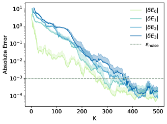
(a) MODMD algorithm

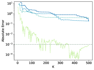
(b) ODMD algorithm

Figure 2: Convergence of eigenenergies for the transverse-field Ising model (TFIM). To obtain eigenenergy estimates $\tilde{E}_{n}$, we fix the (M)ODMD parameters $\frac{K}{d}=\frac{5}{2}$ and $\tilde{\delta}=10^{-2}$ for constructing and thresholding the pair of data matrices $\mathbf{X},\mathbf{X}^{\prime}\in\mathbb{R}^{dI\times(K+1)}$. Gaussian $\mathcal{N}(0,\varepsilon_{\rm noise}^{2})$ noise with $\varepsilon_{\rm noise}=10^{-3}$ is added independently to the real or/and imaginary parts of the matrix elements. The absolute errors, $\lvert\tilde{E}_{n}-E_{n}\rvert$, in the first four eigenenergies of the TFIM Hamiltonian are shown with respect to $K$ proportional to the non-dimensional maximal simulation time. The reference state $\ket{\phi_{0}}$ is an equal superposition of six computational basis states and we use a time step of $\Delta t\approx 0.08$. The shading above the solid/dashed lines shows the standard deviation across trials for each quantity. Left Absolute errors from the multi-observable (MODMD) algorithm with $I=6$, where the convergence results are averaged over 20 trials, each involving a Gaussian noise realization and a selection of $I$ random observables. Right. Absolute errors from the single-observable (ODMD) algorithm where the convergence results are averaged over 20 trials, each involving a Gaussian noise realization.

V.1 Condensed-matter physics

We examine the convergence of the ground and excited state eigenenergies of the 1D transverse field Ising model (TFIM) with a total of $L=15$ spins and open boundary conditions. The system Hamiltonian is given by

$$H_{\text{TFIM}}=-J\sum_{i=1}^{L-1}X_{i}X_{i+1}-h\sum_{i=1}^{L}Z_{i},$$ (56)

for coupling constant $J$ and external field strength $h$.

We first demonstrate the performance of MODMD for TFIM parameters fixed at $J=h=1$, examining how the algorithm behaves with varying number of time steps, or equivalently the maximal simulation time. As discussed in Sections II and IV, increasing the dimensions $d$ and $K$ of the data matrix $\mathbf{X}\in\mathbb{R}^{dI\times(K+1)}$ facilitates convergence of the MODMD eigenvalues $\tilde{\lambda}_{n}=\lvert\tilde{\lambda}_{n}\rvert e^{-i\tilde{E}_{n}\Delta t}$ (note that these eigenvalues are not necessarily confined to the unit circle in complex plane) to the eigenphases $\lambda_{n}=e^{-iE_{n}\Delta t}$ of the Hamiltonian. Fig. 2 illustrates this convergence for the first $N_{\rm eig}=4$ eigenenergy estimates. Specifically, we report the absolute error $\lvert\delta E_{n}\rvert=\lvert\tilde{E}_{n}-E_{n}\rvert$ as a function of the dimension $K$, with the ratio $\frac{K}{d}=\frac{5}{2}$ held constant throughout subsequent calculations as this ratio provides near-optimal performance for ODMD [9].

Figure 3: Convergence of the first excited state energy of the TFIM. Absolute error in the first excited state energy is shown as a function of the spectral gap between the ground and the first excited state for fixed $K=500$. The vertical dotted line marks the noise level $\varepsilon_{\rm noise}=10^{-3}$. Convergence results are averaged over 20 trials each involving a Gaussian noise realization and, in the MODMD case, also a selection of $I$ random observables. The shading above the solid/dashed lines shows the standard deviation across trials for each quantity.

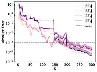
(a) MODMD algorithm

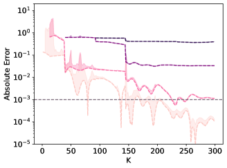
(b) ODMD algorithm

Figure 4: Convergence of eigenenergies for the lithium hydride (LiH) molecule. To obtain eigenenergy estimates $\tilde{E}_{n}$, we fix the (M)ODMD parameters $\frac{K}{d}=\frac{5}{2}$ and $\tilde{\delta}=10^{-2}$ for constructing and thresholding the pair of data matrices $\mathbf{X},\mathbf{X}^{\prime}\in\mathbb{R}^{dI\times(K+1)}$. Gaussian $\mathcal{N}(0,\varepsilon_{\rm noise}^{2})$ noise with $\varepsilon_{\rm noise}=10^{-3}$ is added independently to the real or/and imaginary parts of the matrix elements. The reference state $\ket{\phi_{0}}$ is an equal superposition of the lowest four Hartree-Fock states with identical particle occupation number and we use a time step of $\Delta t\approx 0.33$. The absolute errors, $\lvert\tilde{E}_{n}-E_{n}\rvert$, in the first four eigenenergies of the LiH Hamiltonian are shown with respect to $K$ proportional to the non-dimensional maximal simulation time. Convergence results are averaged over 20 trials of Gaussian noise realizations with shading above the solid/dashed lines showing the standard deviation across trials for each quantity. Left. Absolute errors from the multi-observable (MODMD) algorithm with $I=6$. Right. Absolute errors from the single-observable (ODMD) algorithm.

The left panel illustrates convergence in the multi-observable setting, where we select $I=6$ operators randomly from the set of 1-local Pauli gates and initialize a reference state $\ket{\phi_{0}}$ composed equally of $6$ computational basis states. The use of simple random Pauli observables proves effective here since $(1)$ the TFIM does not preserve the Hamming weight (local bit-flip $X$ does not annihilate $\braket{\phi_{0}}{O_{i}}{\phi_{0}(t)}$) and $(2)$ our reference is a superposition (so local phase-flip $Z$ does not add a trivial $\pm 1$ overall phase). The reference $\ket{\phi_{0}}$ contains relatively small but sufficient overlap with the first few Hamiltonian eigenstates, where the squared overlap sums to $\sum_{n=0}^{N_{\rm eig}-1}\lvert\braket{\psi_{n}}{\phi_{0}}\rvert^{2}\approx 10^{-1}$. This allows for the algorithm to generate an adequate signal without requiring substantial similarity between the reference state and target eigenstates. To stimulate the shadow-induced errors, we additionally introduce Gaussian $\mathcal{N}(0,\varepsilon_{\rm noise}^{2})$ noise with $\varepsilon_{\rm noise}=10^{-3}$ to the multi-observable signal. The absolute energy errors shown are averaged over a total of 20 realizations of both the Gaussian noise and 1-local Pauli observables. For comparison, the right panel displays the single-observable convergence from the standard ODMD algorithm as our benchmark. We observe considerably faster convergence in the excited state energies in MODMD for cases where ODMD nearly stagnates. We highlight that the quantum cost, or total number of shots required, is at most $2(K+d)\log(I)\varepsilon_{\rm noise}^{-2}$, only a factor of $2\log(I)<4$ more than that of ODMD in this case.

The convergence of MODMD naturally divides into two regimes, each defined by a distinct error scaling. The noise level $\varepsilon_{\rm noise}$ essentially determines the crossover between the two convergence regimes. When $\lvert\delta E_{n}\rvert>\varepsilon_{\rm noise}$, we observe an exponentially decaying error typical of the classical subspace methods [49, 53, 51]. Conversely, in the regime where $\lvert\delta E_{n}\rvert<\varepsilon_{\rm noise}$, increasing simulation time leads to slower, algebraic error decay with precision ultimately limited by Heisenberg scaling. This crossover between the exponential and algebraic error decay is shown explicitly within Section E.2. In practice, the onset of the algebraic error behavior can be considerably delayed, for example, via increased and noise-mitigated sampling of classical shadows.

Despite its simplicity, the TFIM is an instructive toy model as it undergoes a quantum phase transition, where the spectral gap between the first two eigenstates can be systematically tuned by varying the $\frac{h}{J}$ ratio. In the thermodynamic limit $L\rightarrow\infty$, the gap closes at $\frac{h}{J}=1$ and increases monotonically with $\frac{h}{J}$. To investigate the gap dependence near a phase transition, we demonstrate the difference in performance between the single-observable (ODMD) and multi-observable (MODMD) algorithms in the presence of near-degenerate target energies. In Fig. 3, we focus on comparing the error $\lvert\delta E_{1}\rvert$ in the first excited energy against the gap $E_{1}-E_{0}$. The convergence results indicate that, in a multi-observable approach, the first excited state energy $E_{1}$ can be accurately estimated if the noise level is slightly smaller than the spectral gap. In contrast, ODMD requires a visibly higher gap-to-noise ratio to achieve a comparable accuracy. This highlights a significant improvement of MODMD in distinguishing near-degenerate eigenstates.

V.2 Quantum chemistry

Electronic structure calculation is a fundamental problem in quantum chemistry. Here we evaluate performance of the MODMD algorithm for molecular Hamiltonians, whose second quantization can be efficiently implemented on the quantum computer. Unlike our condensed-matter example where the first few Hamiltonian eigenvalues map directly to the energy levels of interest, we only consider eigenvalues corresponding to eigenstates with the correct particle number. This symmetry is preserved under time evolution.

Moreover, we construct observables based on the Pauli representation of the Hamiltonian as per Eq. 22, and deterministically select a subset of $I=6$ Pauli operators $P_{\nu}$ with medium-magnitude weights $\kappa_{\nu}$ to maximize the signal independence among the observables. The reference state $\ket{\phi_{0}}$ is prepared as an equal superposition of the lowest four Hartree-Fock states with identical particle occupation number. These Hartree-Fock states are computational basis states readily derived from a mean-field calculation. This choice ensures both a nonzero overlap with the target eigenstates and viability for experimental preparation.

For demonstration, we illustrate MODMD specifically for the lithium hydride (LiH) molecule. Fig. 4 shows the convergence for the first $N_{\rm eig}=4$ eigenenergy estimates, constrained to fixed particle occupation and bond length of $1.59$Å at equilibrium geometry. Similar to the TFIM results in Fig. 2, Fig. 4 exhibits, roughly, an exponential-to-algebraic crossover in the error decay, with a transition occurring around the noise level $\varepsilon_{\rm noise}$. The plateaus for the higher energy levels at intermediate $K$ values can be attributed to the anomalous convergence to different but higher-lying eigenenergies, which we verified numerically. As we approach the interior of the Hamiltonian spectrum, MODMD can resolve the higher excited state energies for sufficiently large $K$, whereas ODMD stagnates.

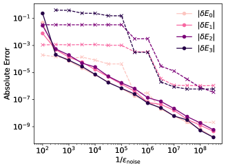
Figure 5: Convergence of eigenergies for LiH under varying noise level. The absolute errors in the first four eigenenergies of the LiH Hamiltonian are shown as a function of the noise level $\varepsilon_{\rm noise}$ for fixed $K=300$ and $\tilde{\delta}=10\varepsilon_{\rm noise}$. Convergence results are averaged over 20 trials of Gaussian noise realizations. The solid lines depict the results for the multi-observable (MODMD) algorithm with $I=6$ and the dashed lines depict the results for the single-observable (ODMD) algorithm.

In Fig. 5 we assess the noise robustness of the MODMD algorithm in our LiH example. Adopting the same hyperparameters as used in Fig. 4, we now fix $K=300$ and vary the noise level $\varepsilon_{\rm noise}$. Importantly, we maintain the SVD threshold $\tilde{\delta}=10\varepsilon_{\rm noise}$ at a consistently larger value. We observe a power law scaling of the absolute error with respect to the noise level, suggesting that a conservative truncation strategy can be used to protect the actual signal from noise across a wide range of noise magnitudes. By comparison, the ODMD algorithm yields larger errors for any given $\varepsilon_{\rm noise}$. Furthermore, reducing noise only improve the ODMD performance when $\varepsilon_{\rm noise}$ reaches small values. In other words, more aggressive truncations must be employed, which may cause a serious loss of the signal information and thereby slower convergence.

VI Conclusion

In this work, we developed a hybrid quantum-classical measurement-driven framework for effectively extracting information about the low-energy eigenspaces of quantum many-body systems. Our novel MODMD approach leverages real-time evolution on quantum hardware and classically unravels multi-dimensional signals, composed of real-time observables, from a limited number of randomized measurements. The simultaneous prediction of many observables leads to accurate estimates of eigenenergies and shallower circuits with shorter evolution time. We explored the theoretical underpinnings of MODMD, which exponentially suppresses spectral error in the low-noise regime. We numerically demonstrated its rapid convergence in the presence of perturbative noise using examples from condensed matter physics and quantum chemistry.

Compared to state-of-the-art real-time approaches, we highlight the unique strengths of our method in addition to its reliable convergence and noise resilience. To our best knowledge, MODMD is among the most resource-efficient for generating real-time signals. This is because (1) we evolve a single reference state for a duration shorter than required by single-observable approaches, where the reduction in the simulation time becomes more substantial as the number of observables included in the signal subspace increases, and (2) the reference state does not have to possess large overlaps with the low energy eigenstates of interest. Furthermore, our classical post-processing consists of solving a simple least-squares problem followed by a truncated SVD, which is ansatz-free and thus circumvents an exponential growth in optimization costs, whether quantum or classical, associated with the number of desired eigenenergies.

In fact, our MODMD framework is capable of retrieving ground and excited state properties beyond eigenenergy levels, demonstrating an extensive and timely application of the low-rank shadow. Building upon recent theoretical progress in adaptive time scheduling, we finally comment that our algorithm may in principle saturate the optimal Heisenberg-limited scaling for phase estimation (here the multi-eigenvalue estimation) under some additional spectral gap assumptions [16]. This promising prospect warrants further analysis in the future work.

Appendix

Appendix A Shadow under locally scrambling dynamics

Here we adopt a dynamical perspective on the efficient generation of the classical shadow, which introduces random scrambling via real-time evolution under a disordered local Hamiltonian $H_{s}(t)$. For concreteness, we focus on quantum spin glass, in particular the disordered transverse field Ising model (TFIM) with Hamiltonian,

$$H_{s}(\tau)=-\sum_{\langle i,j\rangle}^{L}J_{ij}(\tau)X_{i}X_{j}-h(\tau)\sum_{i=1}^{L}Z_{i},$$ (57)

where $J_{ij}$ and $h$ set the spin-spin coupling and external field strength respectively. We assume for simplicity that $J_{ij}=\sum_{k}J_{ij,k}{\mathchoice{\raisebox{0.0pt}{$\displaystyle\chi$}}{\raisebox{0.0pt}{$\textstyle\chi$}}{\raisebox{0.0pt}{$\scriptstyle\chi$}}{\raisebox{0.0pt}{$\scriptscriptstyle\chi$}}}_{[\tau_{k},\tau_{k+1})}(\tau)$ and $h=\sum_{k}h_{k}{\mathchoice{\raisebox{0.0pt}{$\displaystyle\chi$}}{\raisebox{0.0pt}{$\textstyle\chi$}}{\raisebox{0.0pt}{$\scriptstyle\chi$}}{\raisebox{0.0pt}{$\scriptscriptstyle\chi$}}}_{[\tau_{k},\tau_{k+1})}(\tau)$ remain piecewise constant in time, with ${\mathchoice{\raisebox{0.0pt}{$\displaystyle\chi$}}{\raisebox{0.0pt}{$\textstyle\chi$}}{\raisebox{0.0pt}{$\scriptstyle\chi$}}{\raisebox{0.0pt}{$\scriptscriptstyle\chi$}}}_{[\tau_{k},\tau_{k+1}]}$ being an indicator function of the $k$th-step interval. To incorporate scrambling disorder, we employ quenched random interactions, e.g., $J_{ij,k}\sim\mathcal{N}(0,\sigma_{J}^{2})$ and $h_{k}\sim\mathcal{N}(0,\sigma_{h}^{2})$. Thus under the time evolution $U_{s}=\prod_{k=K_{s}}^{0}e^{-iH_{s}(\tau_{k})(\tau_{k+1}-\tau_{k})}$, local quantum information gets scrambled and the resulting entanglement produced by the disorder dynamics facilitates the recovery of $\rho_{\Phi}(t)$. We remark that the number of scrambling time steps $K_{s}$ serves the role analogous to the circuit depth when considering Clifford gates [57]. For any integer $T\geq 0$, $\lim_{K_{s}\rightarrow\infty}\mathcal{U}(\{\tau_{k}\}_{0\leq k\leq K_{s}})$ is a $T$-design, whereby its first $T$ statistical moments align with those of the Haar measure. To simulate long-time dynamics, we draw upon our recent tool of algebraic circuit compression [58, 59], particularly suited to a disordered TFIM Hamiltonian $H_{s}(\tau)$ in Eq. 57, to keep the effective depth of the time evolution $U_{s}$ shallow. Remarkably, the depth post compression should exhibit no dependence on the maximal runtime $\tau_{K_{s}}$, therefore allowing a significantly more efficient exploration of the Haar limit.

Appendix B Observable dynamic mode decomposition

The standard dynamic mode decomposition (DMD), originally developed in the field of numerical fluid dynamics, is a measurement-driven approximation for the temporal progression of a classical dynamical system [60, 61, 62, 63, 64]. Specifically, DMD samples the system snapshots at regular time intervals $\Delta t$ and uses them to construct an efficient representation of the full dynamical trajectory. For simplicity, we consider a system whose $N$-dimensional state manifold is $\mathbb{C}^{N}$. The optimal linear approximation for the discretized time step $k\mapsto k+1$ is expressed as the least-squares (LS) relation,

$$\boldsymbol{\phi}_{k+1}\stackrel{{\scriptstyle{\rm LS}}}{{=}}A_{k}\boldsymbol{\phi}_{k},$$ (58)

where $\boldsymbol{\phi}_{k}\in\mathbb{C}^{N}$ specifies the system state at time $k\Delta t$ and $A_{k}\in\mathbb{C}^{N\times N}$ is the system matrix, i.e., the linear operator that minimizes the residual $\|\boldsymbol{\phi}_{k+1}-A_{k}\boldsymbol{\phi}_{k}\|_{2}$ to yield the LS relation above. Similarly, the optimal linear approximation for a sequence of successive snapshots $k=0,1,\ldots,K+1$ can be determined by the solution,

$$\begin{bmatrix}\rule[-0.86108pt]{0.5pt}{12.91663pt}&\rule[-0.86108pt]{0.5pt}{12.91663pt}&&\rule[-0.86108pt]{0.5pt}{12.91663pt}\\ \boldsymbol{\phi}_{1}&\boldsymbol{\phi}_{2}&\cdots&\boldsymbol{\phi}_{K+1}\\ \rule[-0.86108pt]{0.5pt}{12.91663pt}&\rule[-0.86108pt]{0.5pt}{12.91663pt}&&\rule[-0.86108pt]{0.5pt}{12.91663pt}\\ \end{bmatrix}\stackrel{{\scriptstyle{\rm LS}}}{{=}}A\begin{bmatrix}\rule[-0.86108pt]{0.5pt}{12.91663pt}&\rule[-0.86108pt]{0.5pt}{12.91663pt}&&\rule[-0.86108pt]{0.5pt}{12.91663pt}\\ \boldsymbol{\phi}_{0}&\boldsymbol{\phi}_{1}&\cdots&\boldsymbol{\phi}_{K}\\ \rule[-0.86108pt]{0.5pt}{12.91663pt}&\rule[-0.86108pt]{0.5pt}{12.91663pt}&&\rule[-0.86108pt]{0.5pt}{12.91663pt}\\ \end{bmatrix},$$ (59)

where the system matrix $A$ minimizes the sum of squared residuals over the length-$K$ sequence. The linear flow described by Eq. 59 naturally generates approximate dynamics $\boldsymbol{\phi}_{\rm DMD}(t)=A^{\frac{t}{\Delta t}}\boldsymbol{\phi}_{0}$ governed by eigenmodes of $A$. DMD-based approaches can be remarkably effective despite their formal simplicity, since they are rooted in the general Koopman operator theory developed to describe the behavior of general (non)linear dynamical systems [42, 43, 44, 46, 47].

The standard DMD approach described above for classical dynamics cannot be immediately translated to quantum dynamics. The DMD approximation of the system evolution would require complete knowledge of the system state, as specified by an $N$-dimensional complex vector at each time step. However, we do not have direct access to the full many-body quantum state. Instead, we can only access the state of a quantum system via measurement sampling of observables . To address this challenge, we employ a technique motivated by Takens’ embedding theorem [66, 67, 68] to obtain an effective state vector consisting of an operator measured at a sequence of successive times. We reformulate the linear model underpinning DMD in terms of these observable-vectors to approximate the system dynamics.

Takens’ embedding theorem [66, 67] establishes a connection between the manifold of states, which an observer cannot directly access, and time-delayed measurements of an observable. In particular, the theorem asserts, under generous conditions, that a state on an $N$-dimensional (sub)manifold can be completely determined using a sequence of at most $d_{\star}\leq 2N+1$ time-delayed observables. This correspondence reads

$$\boldsymbol{\phi}(t)\leftrightarrow\boldsymbol{o}_{t,d_{\star}}=\begin{bmatrix}o(t)\\ o(t+\Delta\tau)\\ \vdots\\ o(t+(d_{*}-1)\Delta\tau)\end{bmatrix},$$ (60)

where $\Delta\tau>0$ is the time delay, $\boldsymbol{\phi}(t)$ is the system state, $o(t)=o[\boldsymbol{\phi}(t)]$ is the measured observable, and $\boldsymbol{o}_{t}$ is the $d_{\star}$-dimensional “observable trajectory” containing the dynamical information. The RHS of Eq. 60 is known as a $d_{\star}$-dimensional delayed embedding of the observable. Takens’ theorem relates the evolution of microscopic degrees of freedom to the evolution history of macroscopic observables, providing a concrete probe into the dynamical properties of the system without direct access to the full states. Here we adopt the term Takens’ embedding technique to refer to the method of applying time delays on the system observables, motivated by the rigorous results of Takens’ embedding theorem.

In anticipation of efficiently leveraging near-term quantum resources, we choose the time delay in Takens’ embedding technique to equal the DMD time interval, i.e., $\Delta\tau=\Delta t$. Given this choice, we then measure the system along time steps $\{t_{k}=k\Delta t\}_{k=0}^{K+1}$ and acquire the sequence of observable trajectories $\{\boldsymbol{o}_{t_{k},d}\}_{k=0}^{K+1}$, each of some length $d\leq d_{\star}$,

$$\boldsymbol{o}_{t_{k},d}=\begin{bmatrix}o(t_{k})\\ o(t_{k+1})\\ \vdots\\ o(t_{k+d-1})\\ \end{bmatrix},\qquad 0\leq k\leq K+1.$$ (61)

By construction, the first $(d-1)$ entries of $\boldsymbol{o}_{t_{k},d}$ are identical to the last $(d-1)$ entries of $\boldsymbol{o}_{t_{k-1},d}$. Consequently, the matrix assembled by arranging successive trajectories $\boldsymbol{o}_{t_{k}}$ as columns

$$\mathbf{X}_{k_{1}\mathrel{\mathop{\mathchar 58\relax}}k_{2}}=\begin{bmatrix}\boldsymbol{o}_{t_{k_{1}},d}&\boldsymbol{o}_{t_{k_{1}+1},d}&\cdots&\boldsymbol{o}_{t_{k_{2}},d}\end{bmatrix},$$ (62)

has a Hankel form, i.e., the matrix elements on each anti-diagonal are equal. In the embedding space, we can identify the closest linear flow,

$$\mathbf{X}_{1\mathrel{\mathop{\mathchar 58\relax}}K+1}\stackrel{{\scriptstyle{\rm LS}}}{{=}}A\mathbf{X}_{0\mathrel{\mathop{\mathchar 58\relax}}K}\implies A=\mathbf{X}_{1\mathrel{\mathop{\mathchar 58\relax}}K+1}(\mathbf{X}_{0\mathrel{\mathop{\mathchar 58\relax}}K})^{+},$$ (63)

where $+$ denotes the Moore–Penrose pseudo-inverse. Here the system matrix $A$ assumes a companion structure with just $d$ free parameters. The approximation to the system dynamics is then stored in the $d$ parameters inferred from measurements of $K+d+1$ delayed observables. We hence name our least-squares embedding in the observable space the observable dynamic mode decomposition (ODMD).

Appendix C Multi-observable dynamic mode decomposition

Recall that the multi-observable system matrix has a characteristic polynomial,

$$\mathcal{C}_{A}(z)={\rm det}(z-A)={\rm det}\left(\sum_{\ell=0}^{d}z^{\ell}A_{\ell}\right),$$ (64)

where $A_{d}\equiv{\rm Id}_{I}$. We examine the simpler version of Eq. 12 in which we assume the $d$ matrix blocks,

$$A_{\ell}={\rm Diag}\begin{bmatrix}A_{\ell,11}&&\\ &A_{\ell,22}&&\\ &&\ddots&\\ &&&A_{\ell,II}\\ \end{bmatrix},$$ (65)

to be diagonal with $A_{\ell,ij}\equiv 0$ for $i\neq j$. In this case, the multivariate residual is

$$\overrightarrow{{\rm Res}}_{k}(A)=\sum_{\ell=0}^{d}A_{\ell}\vec{s}_{\ell+k} =\sum_{\ell=0}^{d}A_{\ell}\sum_{n=0}^{N-1}\vec{c}_{n}\lambda_{n}^{\ell+k}=\sum_{n=0}^{N-1}\lambda_{n}^{k}\sum_{\ell=0}^{d}\lambda_{n}^{\ell}A_{\ell}\vec{c}_{n}=\sum_{n=0}^{N-1}\lambda_{n}^{k}\sum_{i=1}^{I}c_{n,i}\left(\sum_{\ell=0}^{d}\lambda_{n}^{\ell}A_{\ell,ii}\right)\vec{e}_{i},$$ (66)

$$=\sum_{n=0}^{N-1}\lambda_{n}^{k}\sum_{i=1}^{I}c_{n,i}\mathcal{C}_{A|i}(\lambda_{n})\vec{e}_{i}=\sum_{i=1}^{I}\left(\sum_{n=0}^{N-1}c_{n,i}\lambda_{n}^{k}\mathcal{C}_{A|i}(\lambda_{n})\right)\vec{e}_{i},$$ (67)

where Eq. 66 directly follows from the submatrices $A_{\ell}$ being diagonal and $\vec{e}_{i}$ denotes the canonical basis vector of $\mathbb{C}^{I}$. Moreover, we define in Eq. 67 the $I$ single-observable characteristic polynomials,

$$\mathcal{C}_{A|i}(z)=\sum_{\ell=0}^{d}z^{\ell}A_{\ell,ii}=\prod_{\ell=0}^{d-1}\left(z-\tilde{\lambda}_{\ell|i}\right),$$ (68)

each with $d$ roots $\tilde{\lambda}_{\ell|i}(A_{0,ii},A_{1,ii},\cdots,A_{d-1,ii})$. Clearly, Eq. 67 indicates that the multivariate residual admits $I$ decoupled components corresponding to the different observables. Minimizing the total residual, $\lVert\overrightarrow{{\rm Res}}_{k}(A)\rVert_{2}$, is hence equivalent to minimizing each of the $I$ observable residuals, $\big{\lvert}\sum_{n=0}^{N-1}c_{n,i}\lambda_{n}^{k}\mathcal{C}_{A|i}(\lambda_{n})\big{\rvert}$. This is consistent with the fact that the matrix determinant ${\rm det}(z-A$) factorizes into independent contributions,

$$\mathcal{C}_{A}(z)=\prod_{i=1}^{I}\left(\sum_{\ell=0}^{d}z^{\ell}A_{\ell,ii}\right)=\prod_{i=1}^{I}\mathcal{C}_{A|i}(z),$$ (69)

such that the eigenvalues of $A$ also factorize into clusters based on single-observable residuals. The resulting MODMD estimates are bounded by the $I$ single-observable ODMD estimates, e.g.,

$$\min_{1\leq i\leq I}\lvert\tilde{E}_{i,0}-E_{0}\rvert\leq\lvert\tilde{E}_{0}-E_{0}\rvert\leq\max_{1\leq i\leq I}\lvert\tilde{E}_{i,0}-E_{0}\rvert,$$ (70)

where $\tilde{E}_{0}$ and $\tilde{E}_{i,0}$ designate, respectively, the ground state energy estimate using the entire observable pool (the full system matrix $A$) and a single observable (one row of the system matrix $A_{\ell,ii}$).

More interesting convergence arises when the $I$ observable residuals are coupled and give a total residual,

$$\overrightarrow{{\rm Res}}_{k}(A) =\sum_{n=0}^{N-1}\lambda_{n}^{k}\sum_{i,j=1}^{I}c_{n,j}\left(\sum_{\ell=0}^{d}\lambda_{n}^{\ell}A_{\ell,ij}\right)\vec{e}_{i},$$ (71)

$$=\sum_{i=1}^{I}\left(\sum_{n=0}^{N-1}c_{n,i}\lambda_{n}^{k}\mathcal{C}_{A|i}(\lambda_{n})+\sum_{n=0}^{N-1}\lambda_{n}^{k}\sum_{\ell=0}^{d-1}\lambda_{n}^{\ell}\sum_{j\neq i}^{I}A_{\ell,ij}c_{n,j}\right)\vec{e}_{i},$$ (72)

where we can lower the residual by utilizing the flexibility of off-diagonal elements in the submatrices $A_{\ell}$. For example, the total residual may vanish completely when the multi-observable signal is $d(I-1)$-sparse in the eigenfrequency basis, where, for $1\leq i\leq I$, the coefficients $c_{n,i}$ are supported on at most $d(I-1)$ eigenindices $\mathcal{N}_{i}=\{0\leq n\leq N-1\mathrel{\mathop{\mathchar 58\relax}}c_{n,i}\neq 0\}$. That is, $\max_{1\leq i\leq I}\lvert\mathcal{N}_{i}\rvert\leq d(I-1)$. In this case, a vanishing residual is possible, provided that $(a)$ $\lvert\cup_{i=1}^{I}\mathcal{N}_{i}\rvert\leq d(I-1)$ and $(b)$ the matrix elements $\{A_{\ell,ij}\}_{\ell,j\neq i}$ can be set appropriately such that $\forall 1\leq i\leq I$,

$$\begin{bmatrix}\beta_{0,i1}(1)&\ldots&\beta_{\ell,ij\neq i}(1)&\ldots&\beta_{d-1,iI}(1)\\ \beta_{0,i1}(2)&\ldots&\beta_{\ell,ij\neq i}(2)&\ldots&\beta_{d-1,iI}(2)\\ \vdots&&\ddots&&\vdots\\ \beta_{0,i1}(\lvert\mathcal{N}_{i}\rvert)&\ldots&\beta_{\ell,ij\neq i}(\lvert\mathcal{N}_{i}\rvert)&\ldots&\beta_{d-1,iI}(\lvert\mathcal{N}_{i}\rvert)\\ \beta_{0,11}(1)&\ldots&\beta_{\ell,1j\neq i}(1)&\ldots&\beta_{d-1,1I}(1)\\ \vdots&&&\ddots&\vdots\\ \beta_{0,I1}(\lvert\mathcal{N}_{I}\rvert)&\ldots&\beta_{\ell,Ij\neq i}(\lvert\mathcal{N}_{I}\rvert)&\ldots&\beta_{d-1,II}(\lvert\mathcal{N}_{I}\rvert)\\ \end{bmatrix}\begin{bmatrix}A_{0,i1}\\ A_{0,i2}\\ \vdots\\ A_{\ell,ij}\\ \\ \vdots\\ A_{d-1,iI}\end{bmatrix}=-\begin{bmatrix}\beta_{0,ii}(1)\mathcal{C}_{A|i}\big{(}\lambda_{n_{1}[i]}\big{)}\\ \beta_{0,ii}(2)\mathcal{C}_{A|i}\big{(}\lambda_{n_{2}[i]}\big{)}\\ \vdots\\ \beta_{0,ii}(\lvert\mathcal{N}_{i}\rvert)\mathcal{C}_{A|i}\big{(}\lambda_{n_{\lvert\mathcal{N}_{i}\rvert}[i]}\big{)}\\ 0\\ \vdots\\ 0\end{bmatrix},$$ (73)

where $n_{\xi}[i]$ numerates support eigenindices in the set $\mathcal{N}_{i}$ for observable $O_{i}$, and $\beta_{\ell,ij}(\xi)=\lambda_{n_{\xi}[i]}^{\ell}c_{n_{\xi}[i],j}$. Given $\{A_{\ell,ii}\}_{\ell}$, a formal solution $\{A_{\ell,ij}\}_{\ell,j\neq i}$ to Eq. 73 exists if the matrix on the LHS has a full rank. This directly implies that the total residual may vanish completely for a $dI$-sparse multi-observable signal in the eigenfrequency basis (as expected), because $\{A_{\ell,ii}\}_{\ell}$ can always be chosen so that the single-observable characteristic polynomial $\mathcal{C}_{A|i}(z)$ encompasses the roots $\{\lambda_{n_{\xi}[i]}\}_{\xi}$ corresponding to at most $d$ members of $\mathcal{N}_{i}$. Without additional degrees of freedom from the off-diagonal matrix elements of $A$, the residual only vanishes for a $d$-sparse signal.

We now relax the sparsity assumption on the signal to explore the general case. Observe that

$$\min_{A}\sum_{k=0}^{K}\left\lVert\overrightarrow{{\rm Res}}_{k}(A)\right\rVert^{2}_{2} =\min_{A}\sum_{k=0}^{K}\sum_{i=1}^{I}\left\lvert\sum_{n=0}^{N-1}c_{n,i}\lambda_{n}^{k}\mathcal{C}_{A|i}(\lambda_{n})+\sum_{j\neq i}^{I}\sum_{n=0}^{N-1}c_{n,j}\lambda_{n}^{k}\mathcal{C}_{A|ij}(\lambda_{n})\right\rvert^{2},$$ (74)

$$\leq\min_{\left\{A_{\ell,ii}\mathrel{\mathop{\mathchar 58\relax}}0\leq\ell\leq d-1,1\leq i\leq I\right\}}\sum_{k=0}^{K}\sum_{i=1}^{I}\left\lvert\sum_{n\notin\mathcal{N}_{i}^{\star}}c_{n,i}\lambda_{n}^{k}\mathcal{C}_{A|i}(\lambda_{n})+\sum_{j\neq i}^{I}\sum_{n\notin\mathcal{N}_{i}^{\star}}c_{n,j}\lambda_{n}^{k}\bar{\mathcal{C}}_{A|ij}(\lambda_{n})\right\rvert^{2},$$ (75)

where $\mathcal{C}_{A|ij}(z)=\sum_{\ell=0}^{d}z^{\ell}A_{\ell,ij}\equiv\sum_{\ell=0}^{d-1}z^{\ell}A_{\ell,ij}$ for $j\neq i$ defines a degree-$(d-1)$ polynomial via the off-diagonal matrix elements $\{A_{\ell,ij}\}_{\ell}$, $\mathcal{N}_{i}^{\star}\subset[N]$ is an eigenindex subset of size $\lvert\mathcal{N}_{i}^{\star}\rvert=d(I-1)$, and $\bar{\mathcal{C}}_{A|ij}(z)=\sum_{\ell=0}^{d-1}z^{\ell}A_{\ell,ij}(\mathcal{N}_{i}^{\star};\{A_{\ell,ii}\}_{\ell})$ fixes $\mathcal{C}_{A|ij}(z)$ by evaluating specific coefficients $\{A_{\ell,ij}\}_{\ell}$ such that,

$$\sum_{j\neq i}^{I}c_{n,j}\bar{\mathcal{C}}_{A|ij}(\lambda_{n})=-c_{n,i}\mathcal{C}_{A|i}(\lambda_{n}),\qquad\forall n\in\mathcal{N}_{i}^{\star}.$$ (76)

Resembling Eq. 73, we reserve the notation $n_{\xi}^{\star}[i]$ for the support eigenindices in $\mathcal{N}_{i}^{\star}$. Eq. 76 then holds only if the following coefficient matrix has full rank, i.e.,

$${\rm rank}[\beta_{\mathcal{N}_{i}^{\star}}]={\rm rank}\begin{bmatrix}\beta_{0,i1}^{\star}(1)&\ldots&\beta_{\ell,ij\neq i}^{\star}(1)&\ldots&\beta_{d-1,iI}^{\star}(1)\\ \beta_{0,i1}^{\star}(2)&\ldots&\beta_{\ell,ij\neq i}^{\star}(2)&\ldots&\beta_{d-1,iI}^{\star}(2)\\ \vdots&&\ddots&&\vdots\\ \beta_{0,i1}^{\star}(\lvert\mathcal{N}_{i}^{\star}\rvert)&\ldots&\beta_{\ell,ij\neq i}^{\star}(\lvert\mathcal{N}_{i}^{\star}\rvert)&\ldots&\beta_{d-1,iI}^{\star}(\lvert\mathcal{N}_{i}^{\star}\rvert)\\ \end{bmatrix}=d(I-1),$$ (77)

for $\beta_{\ell,ij}^{\star}(\xi)=\lambda_{n_{\xi}^{\star}[i]}^{\ell}c_{n_{\xi}^{\star}[i],j}$. An arbitrary index set $\mathcal{N}_{i}^{\star}$ can be assigned as long as the full-rank condition is met; ideally, we aim for $\mathcal{N}_{i}^{\star}=\mathcal{N}_{i}^{\star}(\{A_{\ell,ii}\}_{\ell})$ to satisfy the optimal property,

$$\left\lvert\sum_{j=1}^{I}\sum_{n\notin\mathcal{N}_{i}^{\star}}c_{n,j}\lambda_{n}^{k}\bar{\mathcal{C}}_{A|ij}(\lambda_{n})\right\rvert=\min_{\mathcal{N}\subset[N]\mathrel{\mathop{\mathchar 58\relax}}\lvert\mathcal{N}\rvert=d(I-1)}\left\lvert\sum_{j=1}^{I}\sum_{n\notin\mathcal{N}}c_{n,j}\lambda_{n}^{k}\bar{\mathcal{C}}_{A|ij}(\lambda_{n})\right\rvert,$$ (78)

which minimizes the effective residual parametrized by the $d$ diagonal matrix elements $\{A_{\ell,ii}\}_{\ell}$, with $\bar{\mathcal{C}}_{A|ii}(z)=\mathcal{C}_{A|i}(z)$. By the triangle inequality, we can bound the RHS of Eq. 75 as,

$$\left\lvert\sum_{n\notin\mathcal{N}_{i}^{\star}}c_{n,i}\lambda_{n}^{k}\mathcal{C}_{A|i}(\lambda_{n})+\sum_{j\neq i}^{I}\sum_{n\notin\mathcal{N}_{i}^{\star}}c_{n,j}\lambda_{n}^{k}\bar{\mathcal{C}}_{A|ij}(\lambda_{n})\right\rvert\leq\sum_{j=1}^{I}\sum_{n\notin\mathcal{N}_{i}^{\star}}\left\lvert c_{n,j}\bar{\mathcal{C}}_{A|ij}(\lambda_{n})\right\rvert\leq\bar{c}_{i}\sum_{j=1}^{I}\bar{C}_{ij},$$ (79)

where $\bar{c}_{i}=\max_{1\leq j\leq I}\sum_{n\notin\mathcal{N}_{i}^{\star}}\left\lvert c_{n,j}\right\rvert$ and $\bar{C}_{ij}=\max_{n\notin\mathcal{N}_{i}^{\star}}\lvert\bar{\mathcal{C}}_{A|ij}(\lambda_{n})\rvert$. With suitable choices of the reference state $\ket{\phi_{0}}$ and operator pool $\{O_{i}\}_{i=1}^{I}$, we can strategically adjust the coefficients $\{c_{n,i}\}_{n,i}$, therefore controlling the constant $\bar{c}_{i}$ and the conditioning of the matrix $\beta_{\mathcal{N}_{i}^{\star}}$ (or equivalently $\lVert\beta_{\mathcal{N}_{i}^{\star}}^{-1}\rVert_{2}$). Accordingly, for given index sets $\{\mathcal{N}_{i}^{\star}\}_{i}$, we have

$$\begin{split}\min_{\left\{A_{\ell,ii}\mathrel{\mathop{\mathchar 58\relax}}0\leq\ell\leq d-1,1\leq i\leq I\right\}}&\sum_{k=0}^{K}\sum_{i=1}^{I}\left(\bar{c}_{i}\sum_{j=1}^{I}\bar{C}_{ij}\right)^{2}\\ &\leq(K+1)\sum_{i=1}^{I}\bar{c}_{i}^{2}\min_{\left\{A_{\ell,ii}\mathrel{\mathop{\mathchar 58\relax}}0\leq\ell\leq d-1\right\}}\left(\max_{n\notin\mathcal{N}_{i}^{\star}}\big{\lvert}\mathcal{C}_{A|i}(\lambda_{n})\big{\rvert}+\sum_{\ell=0}^{d-1}\sum_{j\neq i}^{I}\left\lvert A_{\ell,ij}(\mathcal{N}_{i}^{\star};\{A_{\ell,ii}\}_{\ell})\right\rvert\right)^{2},\end{split}$$ (80)

where the residual from the off-diagonal matrix elements can be bounded by,

$$\sum_{\ell=0}^{d-1}\sum_{j\neq i}^{I}\left\lvert A_{\ell,ij}(\mathcal{N}_{i}^{\star};\{A_{\ell,ii}\}_{\ell})\right\rvert\leq d(I-1)\max_{n\in\mathcal{N}_{i}^{\star}}\lvert c_{n,i}\rvert\lVert\beta_{\mathcal{N}_{i}^{\star}}^{-1}\rVert_{2}\max_{n\in\mathcal{N}_{i}^{\star}}\big{\lvert}\mathcal{C}_{A|i}(\lambda_{n})\big{\rvert},$$ (81)

using an identity analogous to Eq. 73. To further bound the RHS of Eq. 80, we attempt to tightly approximate the minimizer over the $d$ diagonal matrix elements $\{A_{\ell,ii}\}_{\ell}$, or alternatively over the set of degree-$d$ monic polynomials defined along the circular arc $\mathcal{A}_{\theta}=\{z\in\mathbb{C}\mathrel{\mathop{\mathchar 58\relax}}\mathinner{\!\left\lvert z\right\rvert}=1,{\rm-\theta\leq arg}(z)\leq\theta\}$. In particular let us consider the complex-valued Chebyshev polynomials,

$$\hat{\mathcal{C}}(z)=\operatorname*{arg\,min}_{\mathcal{C}\hskip 0.56917pt\text{monic}\mathrel{\mathop{\mathchar 58\relax}}\hskip 0.56917pt{\rm deg}(\mathcal{C})=d}\sup_{z\in\mathcal{A}_{\theta}}\mathinner{\!\left\lvert\mathcal{C}(z)\right\rvert},$$ (82)

whose parametric representations are explicitly constructible by tools such as Jacobi’s elliptic and theta functions [69]. For notational convenience, we denote $\lVert\mathcal{C}\rVert_{\theta}=\sup_{z\in\mathcal{A}_{\theta}}\mathinner{\!\left\lvert\mathcal{C}(z)\right\rvert}$. Similar to the real-valued Chebyshev polynomials over the interval $[-1,1]$, $\hat{\mathcal{C}}(z)$ retains the minimal-norm property on $\mathcal{A}_{\theta}$, where $\lVert\hat{\mathcal{C}}\rVert_{\theta}\sim 2\sin^{d}(\theta/2)\cos^{2}(\theta/4)$ asymptotically for large $d$ [70]. Setting $\theta_{H}(\Delta t)=(E_{N-1}-E_{0})\Delta t/2$, the total residual decays at least exponentially:

$$\min_{A}\sum_{k=0}^{K}\left\lVert\overrightarrow{{\rm Res}}_{k}(A)\right\rVert^{2}_{2}\leq(K+1)\lVert\hat{\mathcal{C}}\rVert_{\theta_{H}(\Delta t)}^{2}\sum_{i=1}^{I}\bar{c}_{i}^{2}\left[1+d(I-1)\max_{n\in\mathcal{N}_{i}^{\star}}\lvert c_{n,i}\rvert\lVert\beta_{\mathcal{N}_{i}^{\star}}^{-1}\rVert_{2}\right]^{2},$$ (83)

where the prefactor improves significantly, compared to the single-observable case derived in [9], when

$$\max_{1\leq j\leq I}\sum_{n\notin\mathcal{N}_{i}^{\star}}\left\lvert c_{n,j}\right\rvert\ll\frac{1}{\displaystyle 1+d(I-1)\max_{n\in\mathcal{N}_{i}^{\star}}\lvert c_{n,i}\rvert\lVert\beta_{\mathcal{N}_{i}^{\star}}^{-1}\rVert_{2}},\qquad\forall 1\leq i\leq I.$$ (84)

Appendix D Proof of theorems

D.1 Theorem 1

Theorem 1. Let $\tilde{E}_{0}(d)$ be the approximate ground state energy extracted from the $d$-dimensional function subspace spanned by $\{g_{1},\mathcal{K}_{\Delta t}[g_{1}],\cdots,\mathcal{K}_{\Delta t}^{d-1}[g_{1}]\}$. For $d\geq 1$, there exists time step $\Delta t$ such that the error $\delta E_{g}(d)=\tilde{E}_{0}(d)-E_{0}$ is bounded by

$$\delta E_{0}(d)\leq\frac{\mathinner{\!\left\lvert\sin[(E_{N-1}-E_{0})\Delta t]\right\rvert}}{\tilde{\epsilon}_{0\rightarrow 1}^{2(d-1)}\Delta t}\tan^{2}{\Xi},$$ (85)

where $\cos^{2}{\Xi}=\lvert\langle Nf_{0},g_{1}\rangle_{\mu}\rvert^{2}=\lvert\braket{0}{\psi_{0}}\rvert^{2}$ is the squared overlap between the reference function $g_{1}$ and the true ground state $\mathcal{K}_{\Delta t}$-eigenfunction while $\tilde{\epsilon}_{0\rightarrow 1}=1+3(E_{1}-E_{0})\Delta t/2\pi$ $\in[1,2]$ characterizes the normalized spectral gap of the Hamiltonian $H$.

[Proof.] Let us define,

$$\theta(f)=\arg\frac{\langle f,\mathcal{K}_{\Delta t}f\rangle_{\mu}}{\langle f,f\rangle_{\mu}}\in[-\pi,\pi],$$ (86)

which returns the expected dynamical phase factor associated with a function $f$ under Koopman evolution, where $f$ belongs to the invariance subspace ${\rm span}\{f_{n}\}_{n=0}^{N-1}$. Given a suitable symmetrizing spectral shift such that $\mathinner{\!\left\lVert H\right\rVert}\Delta t\leq\pi$, we note that $\theta(f_{0})=\max_{f}\theta(f)=-E_{0}\Delta t$. This variational principle implies,

$$\tilde{E}_{0}(d) =-\frac{1}{\Delta t}\max_{f\in{\rm Kr}_{d}}\theta(f)=-\frac{1}{\Delta t}\max_{p\in\mathcal{P}_{d-1}}\theta(p(\mathcal{K}_{\Delta t})g_{1}),$$ (87)

for which we use ${\rm Kr}_{d}$ to denote our $d$-dimensional function Krylov subspace ${\rm span}\{g_{1},\cdots,\mathcal{K}_{\Delta t}^{d-1}[g_{1}]\}$ and $\mathcal{P}_{d-1}$ the set of degree-$(d-1)$ polynomials over $\mathbb{C}$. By Eq. 45, we recall that $g_{1}$ can be expanded in $N$ orthogonal eigenfunctions $\{f_{n}\}_{n=0}^{N-1}$, i.e.,

$$g_{1}=\sum_{n=0}^{N-1}z_{n}f_{n},$$ (88)

with $\sum_{n=0}^{N-1}\mathinner{\!\left\lvert z_{n}\right\rvert}^{2}=1$. Thus Eq. 87 in the eigenbasis reads,

$$\tilde{E}_{0}(d) =-\frac{1}{\Delta t}\max_{p\in\mathcal{P}_{d-1}}\arg\frac{\langle p(\mathcal{K}_{\Delta t})g_{1},\mathcal{K}_{\Delta t}p(\mathcal{K}_{\Delta t})g_{1}\rangle_{\mu}}{\langle p(\mathcal{K}_{\Delta t})g_{1},p(\mathcal{K}_{\Delta t})g_{1}\rangle_{\mu}},$$ (89)

$$=-\frac{1}{\Delta t}\max_{p\in\mathcal{P}_{d-1}}\arg\frac{\sum_{n=0}^{N-1}\lambda_{n}\mathinner{\!\left\lvert z_{n}p(\lambda_{n})\right\rvert}^{2}}{\sum_{n=0}^{N-1}\mathinner{\!\left\lvert z_{n}p(\lambda_{n})\right\rvert}^{2}},$$ (90)

where $\lambda_{n}=e^{-iE\Delta t}$ label the eigenvalues of the Koopman operator. We note that

$$\max_{p\in\mathcal{P}_{d-1}}\arg\frac{\sum_{n=0}^{N-1}\lambda_{n}\mathinner{\!\left\lvert z_{n}p(\lambda_{n})\right\rvert}^{2}}{\sum_{n=0}^{N-1}\mathinner{\!\left\lvert z_{n}p(\lambda_{n})\right\rvert}^{2}}\geq\max_{p\in\mathcal{P}_{d-1}}\arg\frac{\lambda_{0}\mathinner{\!\left\lvert z_{0}p(\lambda_{0})\right\rvert}^{2}+\lambda_{N-1}\sum_{n=1}^{N-1}\mathinner{\!\left\lvert z_{n}p(\lambda_{n})\right\rvert}^{2}}{\sum_{n=0}^{N-1}\mathinner{\!\left\lvert z_{n}p(\lambda_{n})\right\rvert}^{2}},$$ (91)

by convexity of the circular sector with angle $[-E_{N-1}\Delta t,-E_{0}\Delta t]$ in the complex plane. Then

$$\tilde{E}_{0}(d) \leq-\frac{1}{\Delta t}\max_{p\in\mathcal{P}_{d-1}}\arg\left[\lambda_{0}+(\lambda_{N-1}-\lambda_{0})\frac{\sum_{n=1}^{N-1}\mathinner{\!\left\lvert z_{n}p(\lambda_{n})\right\rvert}^{2}}{\sum_{n=0}^{N-1}\mathinner{\!\left\lvert z_{n}p(\lambda_{n})\right\rvert}^{2}}\right],$$ (92)

$$=-\frac{1}{\Delta t}\arg\left[\lambda_{0}+(\lambda_{N-1}-\lambda_{0})\min_{p\in\mathcal{P}_{d}}\frac{\sum_{n=1}^{N-1}\mathinner{\!\left\lvert z_{n}p(\lambda_{n})\right\rvert}^{2}}{\sum_{n=0}^{N-1}\mathinner{\!\left\lvert z_{n}p(\lambda_{n})\right\rvert}^{2}}\right],$$ (93)

where we observe $\arg(\lambda_{N-1}-\lambda_{0})=\frac{1}{2}[\arg\lambda_{N-1}+\arg(-\lambda_{0})]\leq\arg\lambda_{0}$ assuming $E_{0}\leq 0$ WLOG. To proceed, we seek a family of polynomials defined over the unit circle $\mathbb{S}^{1}=\{z\in\mathbb{C}\mathrel{\mathop{\mathchar 58\relax}}|z|=1\}$ to bound the fraction on the RHS of Eq. 93. Now let us fix some $q\in(0,1]$ and consider the handy choice of complex-valued Rogers-Szegő polynomials [71, 72],

$$W_{d}(z|q)=\begin{cases}1&d=0\\ z+1&d=1\\ (1+z)W_{d-1}(z|q)\\ \hskip 17.07182pt-(1-q^{j-1})zW_{d-2}(z|q)&d\geq 2\end{cases},$$ (94)

over the circle $\mathbb{S}^{1,q}=\{z\mathrel{\mathop{\mathchar 58\relax}}|z|=q^{-1/2}\}$. For simplicity, we rewrite $z=-q^{-1/2}\exp{(-i\vartheta)}$ where $\vartheta\in[-\pi,\pi])$ denotes an angular phase. Here a prefactor of $-1$ is included to periodically translate the polynomials so that $W_{d}(\vartheta|q)$ adapts the symmetry $W_{d}(-\vartheta)=W_{d}(\vartheta)^{\ast}$ (we also omit a conditional dependence of $W_{d}$ on $q$ for notational clarity). Such family of polynomials shares the key properties that $(i)$ $|W_{d}(\vartheta)|$ remains bounded below unity over some angular window $\mathcal{W}=[-\Omega,\Omega]$ $\subset[-\pi,\pi]$ and $(ii)$ $|W_{d}(\vartheta)|$ grows rapidly outside $\mathcal{W}$.

Note that the constant $q$ controls the width of our truncated angular window $\mathcal{W}$. In the limit of $q\rightarrow 1$, one can verify that these polynomials converge to,

$$W_{d}(\vartheta)\rightarrow\sum_{k=0}^{d}\binom{d}{k}\exp{\left[-ik(\vartheta+\pi)\right]},$$ (95)

which simply gives the sum of evenly spaced points along $\mathbb{S}^{1}$ weighted by binomial coefficients. As a consequence, $\sup_{\vartheta}|W_{d}(\vartheta)|\approx 2^{d}$ for $q\approx 1$. To bound the fraction in Eq. 93 tightly, we look for a suitable linear transformation $\mathcal{L}\mathrel{\mathop{\mathchar 58\relax}}\mathbb{S}^{1}\rightarrow\mathbb{S}^{1}$ acting on the $N$ individual eigenphases, $\lambda_{n}=e^{-i\vartheta_{n}(\Delta t)}$, such that $\mathcal{L}$ nudges excited state angles $\vartheta_{n\geq 1}$ all inside the truncated window $\mathcal{W}$ while keeping the ground state angle $\vartheta_{0}$ outside. It is safe to assume $\vartheta_{N-1}-\vartheta_{1}\leq 2\Omega$ and $2\Omega\leq\vartheta_{N-1}-\vartheta_{0}\leq\pi+\Omega$ by adapting a suitable time step size $\Delta t$, e.g.,

$$\Delta t=\sup_{\tau}\Big{\{}\tau\in\mathbb{R}^{+}\mathrel{\mathop{\mathchar 58\relax}}\vartheta_{N-1}(\tau)-\vartheta_{1}(\tau)\leq 2\Omega,\vartheta_{1}(\tau)-\vartheta_{0}(\tau)\leq\Omega^{\rm c}\Big{\}},$$ (96)

with $\Omega^{\rm c}=\pi-\Omega$. Therefore a natural choice of $\mathcal{L}$ is the phase multiplication or angular translation, $\mathcal{L}\mathrel{\mathop{\mathchar 58\relax}}\vartheta\mapsto\vartheta-\Omega+\vartheta_{1}$, which circularly moves $\{\lambda_{n}\}_{n=0}^{N-1}$ so that $\mathcal{L}(\vartheta_{0})\leq-\Omega=\mathcal{L}(\vartheta_{1})\leq-\mathcal{L}(\vartheta_{N-1})$ as desired. With $\mathcal{L}$ chosen above, we establish a variational upper bound on the ground state energy error by substituting the trial polynomials $p=W_{d-1}\circ\mathcal{L}$ into Eq. 93,

$$\tilde{E}_{0}(d) \leq-\frac{1}{\Delta t}\arg\left[\lambda_{0}+(\lambda_{N-1}-\lambda_{0})\frac{\sum_{n=1}^{Q-1}\mathinner{\!\left\lvert z_{n}W_{d-1}(\mathcal{L}(\lambda_{n}))\right\rvert}^{2}}{\sum_{n=0}^{N-1}\mathinner{\!\left\lvert z_{n}W_{d-1}(\mathcal{L}(\lambda_{n}))\right\rvert}^{2}}\right],$$ (97)

$$\leq-\frac{1}{\Delta t}\arg\left[\lambda_{0}+(\lambda_{N-1}-\lambda_{0})\frac{\sum_{n=1}^{Q-1}\mathinner{\!\left\lvert z_{n}W_{d-1}(\Omega)\right\rvert}^{2}}{\mathinner{\!\left\lvert z_{0}W_{d-1}(\mathcal{L}(\lambda_{0}))\right\rvert}^{2}}\right],$$ (98)

$$=-\frac{1}{\Delta t}\arg\left[\lambda_{0}+(\lambda_{N-1}-\lambda_{0})\frac{\sin^{2}{\Xi}}{\mathinner{\!\left\lvert W_{d-1}(\mathcal{L}(\lambda_{0}))\right\rvert}^{2}\cos^{2}{\Xi}}\right],$$ (99)

where in arriving at Eq. 99 we have utilized the property $(i)$ of $W_{d-1}(\vartheta)$ and defined the angle $\Xi$ by $\cos^{2}{\Xi}=|z_{0}|^{2}=\lvert\langle Nf_{0},g_{1}\rangle_{\mu}\rvert^{2}$ which specifies $L^{2}$-projection of our reference function $g_{1}$ onto the ground state eigenfunction. For the limiting case $q=1$, it is rather straightforward to show that $\Omega=\pi/3$ and,

$$\mathinner{\!\left\lvert W_{d}(\mathcal{L}(\lambda_{0}))\right\rvert}^{1/d}=\sqrt{2-2\cos{\left(\vartheta_{1}-\vartheta_{0}+\Omega\right)}}\geq 1+C\epsilon_{0\rightarrow 1},$$ (100)

where $\epsilon_{0\rightarrow 1}=(\vartheta_{1}-\vartheta_{0})/\Omega^{\rm c}=(E_{1}-E_{0})\Delta t/\Omega^{\rm c}$ gives the normalized spectral gap times the time step and $C$ is a constant for which Eq. 100 holds with $\epsilon_{0\rightarrow 1}\in[0,1]$. For example, $C=1$ can be justified by concavity of the LHS of the inequality above with respect to $(\vartheta_{1}-\vartheta_{0})$. Hence we can further bound Eq. 99 using Eq. 100,

$$\tilde{E}_{0}(d) \leq-\frac{1}{\Delta t}\arg\left[\lambda_{0}\left(1-\tilde{\epsilon}_{0\rightarrow 1}^{-2(d-1)}\tan^{2}{\Xi}\right)+\lambda_{N-1}\tilde{\epsilon}_{0\rightarrow 1}^{-2(d-1)}\tan^{2}{\Xi}\right],$$ (101)

$$\leq\frac{1}{\Delta t}\arctan\left[\frac{(1-\zeta)\sin\vartheta_{0}+\zeta\sin\vartheta_{N-1}}{(1-\zeta)\cos\vartheta_{0}+\zeta\cos\vartheta_{N-1}}\right],$$ (102)

$$=E_{0}+\frac{\sin(\vartheta_{N-1}-\vartheta_{0})}{\Delta t}\zeta+\mathcal{O}(\zeta^{2}),$$ (103)

where we have defined $\tilde{\epsilon}_{0\rightarrow 1}=1+C\epsilon_{0\rightarrow 1}>1$ and $\zeta=\tilde{\epsilon}_{0\rightarrow 1}^{-2(d-1)}\tan^{2}{\Xi}$. The last equality can be derived from a Taylor expansion up to leading order in $\zeta$. So we have proved the statement as claimed. $\square$

D.2 Aside: canonical angles

To set up the proof of theorem 2, we first introduce the notion of subspace overlap for our subsequent discussions. [73] Suppose that we have two subspaces $\mathcal{X}$ and $\mathcal{Y}$ of $\mathbb{C}^{N}$ with ${\rm dim}\mathcal{X}\leq{\rm dim}\mathcal{Y}$. Let $B_{\mathcal{X}}\in\mathbb{C}^{N\times{\rm dim}\mathcal{X}}$ and $B_{\mathcal{Y}}\in\mathbb{C}^{N\times{\rm dim}\mathcal{Y}}$ be the orthornormal basis matrices of $\mathcal{X}$ and $\mathcal{Y}$ ($B_{\mathcal{X}}$ and $B_{\mathcal{Y}}$ are thus not unique). The canonical angles between the subspaces are defined as

$$\theta_{\ell}[\mathcal{X},\mathcal{Y}]=\arccos{\sigma_{\ell}}\in[0,\frac{\pi}{2}],\quad 1\leq\ell\leq{\rm dim}\mathcal{X},$$ (104)

where $\sigma_{1}\leq\sigma_{2}\leq\ldots\leq\sigma_{{\rm dim}\mathcal{X}}$ denote the singular values of $B_{\mathcal{X}}^{\dagger}B_{\mathcal{Y}}$. For convenience, we use a diagonal matrix

$$\Theta[\mathcal{X},\mathcal{Y}]=\begin{bmatrix}\theta_{1}&&&\\ &\theta_{2}&&\\ &&\ddots&\\ &&&\theta_{{\rm dim}\mathcal{X}}\end{bmatrix}$$ (105)

to record the set of ${\rm dim}\mathcal{X}$ canonical angles. Notice when ${\rm dim}\mathcal{X}=1$, the canonical angle is determined by the familiar $\ell^{2}$-inner product on the Hilbert space. Here we present elementary and known results [74] that are helpful for deriving the block convergence bound.

Result C.2.1. For $\mathcal{Y}_{0}\subseteq\mathcal{Y}$ with ${\rm dim}\mathcal{Y}_{0}={\rm dim}\mathcal{X}$, $\theta_{\ell}[\mathcal{X},\mathcal{Y}]\leq\theta_{\ell}[\mathcal{X},\mathcal{Y}_{0}]$ and the equality can be saturated.

Result C.2.2. Suppose ${\rm dim}\mathcal{X}={\rm dim}\mathcal{Y}$ and $\theta_{\ell}[\mathcal{X},\mathcal{Y}]\neq\frac{\pi}{2}$.

(a) For $\mathcal{Y}_{0}\subseteq\mathcal{Y}$, there exists unique $\mathcal{X}_{0}\subseteq\mathcal{X}$ with ${\rm dim}\mathcal{X}_{0}={\rm dim}\mathcal{Y}_{0}$ such that $\Pi_{\mathcal{Y}}\mathcal{X}_{0}=\mathcal{Y}_{0}$ for orthogonal projection $\Pi_{\mathcal{Y}}$ onto $\mathcal{Y}$. Moreover,

$$\theta_{\ell}[\mathcal{X}_{0},\mathcal{Y}_{0}]\leq\theta_{\ell}[\mathcal{X},\mathcal{Y}],$$ (106)

for $1\leq\ell\leq{\rm dim}\mathcal{Y}_{0}$ and hence

$$\lVert\sin\Theta[\mathcal{X}_{0},\mathcal{Y}_{0}]\rVert\leq\lVert\sin\Theta[\mathcal{X},\mathcal{Y}]\rVert$$ (107)

for any unitarily invariant norm $\lVert\cdot\rVert$.

(b) For any orthonormal vectors $[y_{1},\ldots,y_{Q}]$ in $\mathcal{Y}$, there exists linearly independent vectors $[x_{1},\ldots,x_{Q}]$ in $\mathcal{X}$ so that $\Pi_{\mathcal{Y}}x_{\ell}=y_{\ell}$ and $(a)$ holds for $\mathcal{X}_{0}={\rm span}\{x_{1},\ldots,x_{Q}\}$ and $\mathcal{Y}_{0}={\rm span}\{y_{1},\ldots,y_{Q}\}$ with ${\rm dim}\mathcal{X}_{0}={\rm dim}\mathcal{Y}_{0}=Q$.

D.3 Theorem 2

Theorem 2. Let $\tilde{E}_{n}(d)$ be the approximate $n$th eigenenergy extracted from the $dI$-dimensional function subspace ${\rm span}\{\vec{g},\mathcal{K}_{\Delta t}[\vec{g}],\cdots,\mathcal{K}_{\Delta t}^{d-1}[\vec{g}]\}$, and $\delta E_{n}(d)=\tilde{E}_{n}(d)-E_{n}$ be the approximation error. Consider the error matrix,

$$\boldsymbol{\Delta}_{I}(d)={\rm diag}\begin{bmatrix}\delta E_{0}(d)&&\\ &&\ddots&\\ &&&\delta E_{I-1}(d)\\ \end{bmatrix},$$ (108)

which contains approximations to the lowest $I$ energies. For $d\geq 1$, there exists time step $\Delta t$ such that the spectral approximation $\boldsymbol{\Delta}_{I}(d)$ is bounded by

$$\lVert\boldsymbol{\Delta}_{I}(d)\rVert_{2}\leq\frac{\mathinner{\!\left\lvert\sin[(E_{N-1}-E_{0})\Delta t]\right\rvert}}{\tilde{\epsilon}_{I-1\mapsto I}^{2(d-1)}\Delta t}\lVert\tan^{2}\Theta\rVert_{2},$$ (109)

for the operator norm $\lVert\cdot\rVert_{2}$. Here $\Theta$ denotes the canonical angle between the two subspaces ${\rm span}\{f_{n}\mathrel{\mathop{\mathchar 58\relax}}0\leq n\leq I-1\}$ and ${\rm span}\{g_{i}\mathrel{\mathop{\mathchar 58\relax}}1\leq i\leq I\}$, which generalizes the squared overlap in theorem 1 (see Sections D.2 and D.3). In the denominator, $\tilde{\epsilon}_{I-1\mapsto I}\in[1,2]$ depends on the $I$th spectral gap $(E_{I}-E_{I-1})$ of the Hamiltonian $H$.

[Proof.] It suffices to establish the more general result for the error matrix $\boldsymbol{\Delta}={\rm diag}[\delta E_{n_{1}}(d),\delta E_{n_{1}+1}(d),\ldots,\delta E_{n_{2}}(d)]$ for $n_{2}-n_{1}+1=I$. From here on, we will use the operator norm as a specific example of a unitarily invariant norm by setting $\lVert\cdot\rVert=\lVert\cdot\rVert_{2}$. Our key contribution lies in extending the proof of the theorem, building on existing results for block Krylov methods [73], to the real-time setting. Applying result C.2.2(b), we know there exists $B_{I}=[x_{1},\ldots,x_{I}]$ with ${\rm span}B_{I}={\rm span}\{g_{1},\ldots,g_{I}\}$ so that $\Pi_{{\rm invariant~{}subspace}}B_{I}=[f_{n_{1}},\ldots,f_{n_{2}}]$. WLOG we assume that $B_{I}\mapsto B_{I}(B_{I}^{\dagger}B_{I})^{-1/2}$ has orthonormal columns, i.e., $\braket{x_{i},x_{j}}_{\mu}=\delta_{ij}$ for $1\leq i,j\leq I$. For a degree-$(d-1)$ polynomial $p$, we define

$$R_{I}=p(\mathcal{K}_{\Delta t})B_{I}=\sum_{n=0}^{N-1}f_{n}p(\lambda_{n})f_{n}^{\dagger}B_{I},$$ (110)

where the dual $f_{n}^{\dagger}$ are defined with respect to the functional inner product $\braket{\cdot,\cdot}_{\mu}$. We will further write the equality above as

$$R_{I}=Fp(\Lambda)F^{\dagger}B_{I}=\left[F_{a}p(\Lambda_{a})F^{\dagger}_{a}+F_{b}p(\Lambda_{b})F^{\dagger}_{b}+F_{c}p(\Lambda_{c})F^{\dagger}_{c}\right]B_{I},$$ (111)

where $F=[F_{a}~{}F_{b}~{}F_{c}]$ and $\Lambda=\Lambda_{a}\oplus\Lambda_{b}\oplus\Lambda_{c}$ contain the $N$ Koopman eigenfunctions and eigenvalues respectively in a block form. Here we use three subscripts $a$, $b$, and $c$ to label the partition of Hamiltonian spectrum into three disjoint blocks with energies below $E_{n_{1}}$, from $E_{n_{1}}$ to $E_{n_{2}}$, and above $E_{n_{2}}$. In particular, the middle block $b$ is represented by $F_{b}=[f_{n_{1}},\ldots,f_{n_{2}}]$ and $\Lambda_{b}={\rm diag}[\lambda_{n_{1}},\ldots,\lambda_{n_{2}}]$.

By our construction, $F_{b}^{\dagger}B_{I}$ is nonsingular so

$$R_{I}(F_{b}^{\dagger}R_{I})^{-1}=R_{I}\left[p(\Lambda_{b})F_{b}^{\dagger}B_{I}\right]^{-1}=F_{a}p(\Lambda_{a})F^{\dagger}_{a}B_{I}\left[p(\Lambda_{b})F_{b}^{\dagger}B_{I}\right]^{-1}+F_{b}+F_{c}p(\Lambda_{c})F^{\dagger}_{c}B_{I}\left[p(\Lambda_{b})F_{b}^{\dagger}B_{I}\right]^{-1},$$ (112)

whenever $p(\Lambda_{b})$ is nonsingular by suitable choice of the polynomial $p$. Since ${\rm span}R_{I}$ is clearly a subspace of the Krylov subspace ${\rm Kr}_{d,I}\mathrel{\mathop{\mathchar 58\relax}}={\rm span}\{\vec{g},\cdots,\mathcal{K}_{\Delta t}^{d-1}[\vec{g}]\}$, result C.2.1 implies

$$\left\lVert\tan\Theta\left[{\rm span}F_{b},{\rm Kr}_{d,I}\right]\right\rVert \leq\Big{\lVert}\tan\Theta[{\rm span}F_{b},{\rm span}R_{I}]\Big{\rVert},$$ (113)

$$=\left\lVert\sin{\Theta[{\rm span}F_{b},{\rm span}R_{I}]}\left(\cos{\Theta[{\rm span}F_{b},{\rm span}R_{I}]}\right)^{-1}\right\rVert,$$ (114)

$$=\left\lVert[F_{a}~{}F_{c}]^{\dagger}R_{I}(F_{b}^{\dagger}R_{I})^{-1}\right\rVert=\left\lVert\begin{bmatrix}p(\Lambda_{a})&0\\ 0&p(\Lambda_{c})\end{bmatrix}\begin{bmatrix}F_{a}^{\dagger}B_{I}(F_{b}^{\dagger}B_{I})^{-1}\\ F_{c}^{\dagger}B_{I}(F_{b}^{\dagger}B_{I})^{-1}\end{bmatrix}p(\Lambda_{b})^{-1}\right\rVert,$$ (115)

$$\leq\left\lVert\begin{bmatrix}p(\Lambda_{a})&0\\ 0&p(\Lambda_{c})\end{bmatrix}\right\rVert\left\lVert p(\Lambda_{b})^{-1}\right\rVert\left\lVert\begin{bmatrix}F_{a}^{\dagger}B_{I}(F_{b}^{\dagger}B_{I})^{-1}\\ F_{c}^{\dagger}B_{I}(F_{b}^{\dagger}B_{I})^{-1}\end{bmatrix}\right\rVert,$$ (116)

$$\leq\frac{\displaystyle\max_{n<n_{1}\lor n>n_{2}}\lvert p(\lambda_{n})\rvert}{\displaystyle\min_{n_{1}\leq n\leq n_{2}}\lvert p(\lambda_{n})\rvert}\left\lVert\tan\Theta[{\rm span}F_{b},{\rm span}B_{I}]\right\rVert,$$ (117)

where Eq. 115 results from the substitution of Eq. 112.

The inequality above characterizes the convergence of the Krylov subspace (towards to the target eigenstates), and our task is to choose a polynomial $p$ that can tightly bound the fraction in Eq. 117. As in Section D.1, we exploit the Rogers-Szegő polynomials $W_{d-1}(z|q)$ and work in the limit $q=1$ to derive relevant results. For $n_{2}=N-1$, let us consider the polynomial

$$p(z)=\frac{W_{d-1}(e^{-i\varphi}z)}{W_{d-1}(e^{-i\varphi}\lambda_{n_{1}})},$$ (118)

where $e^{-i\varphi}$ is a constant phase offset shifting the angles $\vartheta_{n<n_{1}}$ (recall that $\vartheta_{n}=E_{n}\Delta t$) inside the window $\mathcal{W}=[-\Omega,\Omega]$ while keeping the angles $\vartheta_{n_{1}\leq n\leq n_{2}}$ outside $\mathcal{W}$. In this case, observe that

$$\min_{n_{1}\leq n\leq n_{2}}\lvert p(\lambda_{n})\rvert =\lvert p(\lambda_{n_{1}})\rvert=1,$$ (119)

$$\max_{n<n_{1}\lor n>n_{2}}\lvert p(\lambda_{n})\rvert =\max_{n<n_{1}}\lvert p(\lambda_{n})\rvert\leq\frac{1}{\left\lvert{W_{d-1}(e^{-i\varphi}\lambda_{n_{1}})}\right\rvert}.$$ (120)

By employing suitable time step size $\Delta t$, e.g., that from Eq. 96, we assume $\vartheta_{n_{1}-1}-\vartheta_{0}\leq 2\Omega$ and $2\Omega\leq\vartheta_{N-1}-\vartheta_{0}\leq\pi+\Omega$. Specifically, $\varphi=\Omega-\vartheta_{n_{1}-1}$ circularly shifts the eigenphases $\{\lambda_{n}\}_{n=0}^{N-1}$. This ensures that $\mathinner{\!\left\lvert\varphi+\vartheta_{0}\right\rvert}\leq\varphi+\vartheta_{n_{1}-1}=\Omega\leq\varphi+\vartheta_{n_{1}}$ as intended. From theorem 1, we recall $\Omega=\pi/3$ and $\lvert W_{d-1}(e^{-i\varphi}\lambda_{n_{1}})\rvert^{1/(d-1)}\geq 1+C\epsilon_{n_{1}-1\mapsto n_{1}}$ where $\epsilon_{n_{1}-1\mapsto n_{1}}=3(E_{n_{1}}-E_{n_{1}-1})\Delta t/2\pi$ encodes the normalized $n_{1}$th energy gap and $C$ is some appropriate constant that can be set to $1$ (c.f. Eq. 100). This immediately implies an exponential convergence to the eigenspaces,

$$\left\lVert\tan\Theta\left[{\rm span}F_{b},{\rm Kr}_{d,I}\right]\right\rVert\leq\frac{1}{\tilde{\epsilon}_{n_{1}-1\mapsto n_{1}}^{(d-1)}}\left\lVert\tan\Theta\left[{\rm span}F_{b},{\rm span}\{g_{1},\ldots,g_{I}\}\right]\right\rVert,$$ (121)

for the base case $n_{2}=N-1$. When $n_{2}<N-1$, we consider the polynomial $p=p_{1}\cdot p_{2}$ with

$$p_{1}(z)=\frac{W_{d-N+n_{2}}(e^{-i\varphi}z)}{W_{d-N+n_{2}}(e^{-i\varphi}\lambda_{n_{1}})},$$ (122)

and

$$p_{2}(z)=\prod_{n=n_{2}+1}^{N-1}\frac{z-\lambda_{n}}{\lambda_{n_{2}}-\lambda_{n}},$$ (123)

where $p$ is factorized into lower order polynomials $p_{1}$ of degree $(d-N+n_{2})$ and $p_{2}$ of degree $(N-n_{2}-1)$. Observe that by design $p(\lambda_{n})=0$ for $n\geq n_{2}+1$ and thus

$$\min_{n_{1}\leq n\leq n_{2}}\lvert p(\lambda_{n})\rvert \geq\min_{n_{1}\leq n\leq n_{2}}\lvert p_{1}(\lambda_{n})\rvert\min_{n_{1}\leq n\leq n_{2}}\left\lvert p_{2}(\lambda_{n})\right\rvert=\min_{n_{1}\leq n\leq n_{2}}\prod_{m=n_{2}+1}^{N-1}\left\lvert\frac{\lambda_{n}-\lambda_{m}}{\lambda_{n_{2}}-\lambda_{m}}\right\rvert,$$ (124)

$$\max_{n<n_{1}\lor n>n_{2}}\lvert p(\lambda_{n})\rvert \leq\max_{n<n_{1}}\lvert p_{1}(\lambda_{n})\rvert\max_{n<n_{1}}\lvert p_{2}(\lambda_{n})\rvert\leq\frac{1}{\left\lvert{W_{d-N+n_{2}}(e^{-i\varphi}\lambda_{n_{1}})}\right\rvert}\max_{n<n_{1}}\prod_{m=n_{2}+1}^{N-1}\left\lvert\frac{\lambda_{n}-\lambda_{m}}{\lambda_{n_{2}}-\lambda_{m}}\right\rvert,$$ (125)

which directly follows from applying our base case result to the eigensector $\{\lambda_{n}\}_{n=0}^{n_{2}}$. Note that our argument requires $d\geq N-n_{2}$: a symmetric bound can be readily established using the exact same argument with the roles of $n_{1}$ and $n_{2}$ exchanged, i.e., for $d\geq n_{1}+1$, upon a spectral flip $H\mapsto-H$.

Now we proceed to analyze the convergence of the Krylov energy approximation. For simplicity, we focus again on approximating from below Hamiltonian eigenvalues $E_{n}\lesssim E_{N-1}$ near the right edge of the spectrum. The argument for approximating from above eigenvalues near the left edge of the spectrum can be easily adapted with a spectral flip. We observe that up to the trivial spectral rotation $\mathcal{K}_{\Delta t}\mapsto\lambda_{n_{2}}^{-1}\mathcal{K}_{\Delta t}$ leaving the functional Krylov subspace invariant, we can assume WLOG $E_{n_{2}-1}\leq 0<E_{n_{2}+1}$ for the remainder of the proof. For $V_{0}\mathrel{\mathop{\mathchar 58\relax}}=R_{I}(F_{b}^{\dagger}R_{I})^{-1}$, we first construct $V_{-}=V_{0}(V_{0}^{\dagger}V_{0})^{-1/2}$, which contains orthonormal columns. This allows us to introduce eigenvalues, $\hat{\lambda}_{n}=\lvert\hat{\lambda}_{n}\rvert e^{-i\hat{E}_{n}\Delta t}$ for $n_{1}\leq n\leq n_{2}$, of the ${\rm span}V_{0}$-projected Koopman operator $V^{\dagger}_{-}\mathcal{K}_{\Delta t}V_{-}$, with the ordering ${\rm arg}(\hat{\lambda}_{n_{1}})\geq\ldots\geq{\rm arg}(\hat{\lambda}_{n_{2}})$. These eigenvalues depend explicitly on choices of the degree-$(d-1)$ polynomial $p$ (as $R_{I}$ does). Since ${\rm span}V_{0}\subseteq{\rm Kr}_{d,I}$ irrespective of $p$, the variational principle gives

$$\hat{E}_{n}(d)\leq\tilde{E}_{n}(d)\leq E_{n}\implies 0\leq\delta E_{n}(d)\leq E_{n}-\hat{E}_{n}(d),\quad n_{1}\leq n\leq n_{2}.$$ (126)

The variational characterization, as we shall see, leads to an upper bound on the spectral error

$$\boldsymbol{\Delta}_{I,n_{1},n_{2}}={\rm diag}\begin{bmatrix}\delta E_{n_{1}}&&\\ &\ddots&\\ &&\delta E_{n_{2}}\end{bmatrix},$$ (127)

which generalizes $\boldsymbol{\Delta}_{I}$ in theorem 2 ($\boldsymbol{\Delta}_{I,n_{1},n_{2}}=\boldsymbol{\Delta}_{I}$ when $n_{1}=N-I$ and $n_{2}=N-1$). With our previous assumption $E_{n_{2}}=0$, we have $\hat{E}_{n}\leq 0$ for $n_{1}\leq n\leq n_{2}$. Consequently, $\forall x\in\mathbb{C}^{I}$

$$-\frac{1}{\Delta t}\theta(V_{0}x)=-\frac{1}{\Delta t}{\rm arg}\frac{\braket{V_{0}x,\mathcal{K}_{\Delta t}V_{0}x}_{\mu}}{\braket{V_{0}x,V_{0}x}_{\mu}}\leq 0,$$ (128)

where we adopt the same notation as in theorem 1 (c.f. Eq. 86). By unfolding $V_{0}$ via Eq. 112, we arrive at

$$V_{0}^{\dagger}\mathcal{K}_{\Delta t}V_{0} =G_{a}^{\dagger}\Lambda_{a}G_{a}+\Lambda_{b}+G_{c}^{\dagger}\Lambda_{c}G_{c},$$ (129)

and

$$V_{0}^{\dagger}V_{0} =G_{a}^{\dagger}G_{a}+{\rm Id}_{I}+G_{c}^{\dagger}G_{c},$$ (130)

for $G_{a}=p(\Lambda_{a})F_{a}^{\dagger}B_{I}[p(\Lambda_{b})F_{b}^{\dagger}B_{I}]^{-1}$ and $G_{c}=p(\Lambda_{c})F_{c}^{\dagger}B_{I}[p(\Lambda_{b})F_{b}^{\dagger}B_{I}]^{-1}$. Substituting Eqs. 129 and 130 into the variational inequality, we can derive

$$-\frac{1}{\Delta t}{\rm arg}\frac{x^{\dagger}(G^{\dagger}_{a}\Lambda_{a}G_{a}+\eta_{b}\lambda_{n_{2}}{\rm Id}_{I})x}{x^{\dagger}x}-\frac{1}{\Delta t}{\rm arg}\frac{x^{\dagger}\Lambda_{b}x}{x^{\dagger}x}+\frac{1}{\Delta t}{\rm arg}\lambda_{n_{2}} \leq-\frac{1}{\Delta t}{\rm arg}\frac{x^{\dagger}(G_{a}^{\dagger}\Lambda_{a}G_{a}+\Lambda_{b})x}{x^{\dagger}x},$$ (131)

$$\leq-\frac{1}{\Delta t}{\rm arg}\frac{x^{\dagger}(G_{a}^{\dagger}\Lambda_{a}G_{a}+\Lambda_{b}+G_{c}^{\dagger}\Lambda_{c}G_{c})x}{x^{\dagger}(G_{a}^{\dagger}G_{a}+{\rm Id}_{I}+G_{c}^{\dagger}G_{c})x},$$ (132)

$$=-\frac{1}{\Delta t}{\rm arg}\frac{\braket{V_{0}x,\mathcal{K}_{\Delta t}V_{0}x}_{\mu}}{\braket{V_{0}x,V_{0}x}_{\mu}}\leq 0,$$ (133)

where $\eta_{b}=\inf_{x\in\mathbb{C}^{I}\mathrel{\mathop{\mathchar 58\relax}}x^{\dagger}x=1}\lVert x^{\dagger}\Lambda_{b}x\rVert$ is a constant of $\mathcal{O}(1)$ when $\vartheta_{n_{2}}-\vartheta_{n_{1}}<\pi/2$, and we recall that $E_{n_{2}}=0\implies\lambda_{n_{2}}=1$ in our current setting. In particular, the inequality Eq. 131 above holds since for any unit vector $x\mapsto\frac{x}{\sqrt{x^{\dagger}x}}$,

$${\rm arg}\frac{\displaystyle\lambda_{n_{2}}x^{\dagger}(G^{\dagger}_{a}\Lambda_{a}G_{a}+\Lambda_{b})x}{\displaystyle x^{\dagger}(G^{\dagger}_{a}\Lambda_{a}G_{a}+\eta_{b}\lambda_{n_{2}}{\rm Id}_{I})x\cdot x^{\dagger}\Lambda_{b}x}={\rm arg}\frac{\displaystyle\frac{\lambda_{n_{2}}}{x^{\dagger}\Lambda_{b}x}+\frac{\lambda_{n_{2}}}{x^{\dagger}G^{\dagger}_{a}\Lambda_{a}G_{a}x}}{\displaystyle 1+\frac{\eta_{b}\lambda_{n_{2}}}{x^{\dagger}G^{\dagger}_{a}\Lambda_{a}G_{a}x}}\leq{\rm arg}\frac{\displaystyle\frac{\lambda_{n_{2}}}{x^{\dagger}\Lambda_{b}x}+\frac{\lambda_{n_{2}}}{x^{\dagger}G^{\dagger}_{a}\Lambda_{a}G_{a}x}}{\displaystyle 1+\frac{\lVert x^{\dagger}\Lambda_{b}x\rVert\lambda_{n_{2}}}{x^{\dagger}G^{\dagger}_{a}\Lambda_{a}G_{a}x}}\leq 0,$$ (134)

where the numerator has a smaller phase than the denominator. The inequality Eq. 133, on the other hand, follows from our basic assumption that $E_{n}\leq 0$ for $n\leq n_{2}$. The inequalities indicate that the $G_{a}^{\dagger}\Lambda_{a}G_{a}$-eigenvalues, denoted as $\bar{\lambda}_{n}$ for $n_{1}\leq n\leq n_{2}$ (with the eigenvalues ordered by decreasing arguments), are related to the $V^{\dagger}_{-}\mathcal{K}_{\Delta t}V_{-}$-eigenvalues through

$$-\frac{1}{\Delta t}{\rm arg}(\bar{\lambda}_{n}+\eta_{b}\lambda_{n_{2}})+E_{n}-E_{n_{2}}\leq\hat{E}_{n},\quad n_{1}\leq n\leq n_{2}.$$ (135)

Consequently, we may relax the error bound in Eq. 126,

$$\delta E_{n}\leq E_{n}-\hat{E}_{n} \leq\frac{1}{\Delta t}{\rm arg}(\bar{\lambda}_{n}+\eta_{b}\lambda_{n_{2}})+E_{n_{2}},$$ (136)

$$\leq\frac{1}{\Delta t}{\rm arg}\left[\lambda_{0}\frac{e^{\dagger}_{n}G^{\dagger}_{a}G_{a}e_{n}}{\eta_{b}e^{\dagger}_{n}e_{n}}+\lambda_{n_{2}}\right]+E_{n_{2}},$$ (137)

$$\leq\frac{1}{\Delta t}{\rm arg}\left[\lambda_{0}\frac{y^{\dagger}_{n}G^{\dagger}_{a}G_{a}y_{n}}{\eta_{b}y^{\dagger}_{n}y_{n}}+\lambda_{n_{2}}\right]+E_{n_{2}},$$ (138)

where $e_{n}$ denotes the eigenvector of $G^{\dagger}_{a}\Lambda_{a}G_{a}$ corresponding to $\bar{\lambda}_{n}$ and $y_{n}$ the eigenvector of $G^{\dagger}_{a}G_{a}$ corresponding to the $(n-n_{1}+1)$th largest eigenvalue. Importantly, we remark that Eqs. 131 and 138 can be established without phase ambiguity of $2\pi\mathbb{Z}$ by choosing suitable time step size $\Delta t$.

We therefore seek a tight bound on the eigenvalues of $G_{a}^{\dagger}G_{a}$ (or equivalently the singular values of $G_{a}$). Notice that the singular values of $p(\Lambda_{a})^{-1}\cdot G_{a}\cdot p(\Lambda_{b})=p(\Lambda_{a})^{-1}\cdot p(\Lambda_{a})F_{a}^{\dagger}B_{I}[p(\Lambda_{b})F_{b}^{\dagger}B_{I}]^{-1}\cdot p(\Lambda_{b})=F_{a}^{\dagger}B_{I}[F_{b}^{\dagger}B_{I}]^{-1}$ are bounded above by the singular values of the canonical tangents (c.f. Eq. 117)

$$\tan\Theta[{\rm span}F_{b},{\rm span}B_{I}]=\begin{bmatrix}F_{a}^{\dagger}B_{I}(F_{b}^{\dagger}B_{I})^{-1}\\ F_{c}^{\dagger}B_{I}(F_{b}^{\dagger}B_{I})^{-1}\end{bmatrix}.$$ (139)

This allows us to effectively control the spectral radius of $G_{a}^{\dagger}G_{a}$,

$$\lVert G^{\dagger}_{a}G_{a}\rVert \leq\lVert p(\Lambda_{a})\rVert^{2}\lVert p(\Lambda_{b})^{-1}\rVert^{2}\left\lVert\tan^{2}\Theta[{\rm span}F_{b},{\rm span}B_{I}]\right\rVert,$$ (140)

$$=\frac{\displaystyle\max_{n<n_{1}}\lvert p(\lambda_{n})\rvert^{2}}{\displaystyle\min_{n_{1}\leq n\leq n_{2}}\lvert p(\lambda_{n})\rvert^{2}}\left\lVert\tan^{2}\Theta[{\rm span}F_{b},{\rm span}B_{I}]\right\rVert,$$ (141)

where it suffices to identify a degree-$(d-1)$ polynomial $p$ that tightly bounds the fraction on the RHS of the expression above. In addition, here $p$ must satisfy the key orthogonality constraints,

$$\tilde{f}_{n}^{\dagger}R_{I}=[0~{}0~{}\ldots~{}0],\quad n_{2}+1\leq n\leq N-1,$$ (142)

where $\tilde{f}_{n}\in{\rm Kr}_{d,I}$ denotes the approximate eigenfunction corresponding to the Krylov eigenvalue $\tilde{\lambda}_{n}=\lvert\tilde{\lambda}_{n}\rvert e^{-i\tilde{E}_{n}\Delta t}$. The set of $(N-n_{2})$ constraints ensure that ${\rm span}R_{I}=p(\mathcal{K}_{\Delta t}){\rm span}B_{I}=p(\mathcal{K}_{\Delta t}){\rm span}\{g_{1},\ldots,g_{I}\}$ belongs to the correct eigensector of the Krylov subspace. Let us consider the familiar polynomial $p=p_{1}\cdot p_{2}$ with $p_{1}$ of degree-$(d-N+n_{2})$ and $p_{2}$ of degree $(N-n_{2}-1)$ given by

$$p_{1}(z)=\frac{W_{d-N+n_{2}}(e^{-i\varphi}z)}{W_{d-N+n_{2}}(e^{-i\varphi}\lambda_{n_{1}})},$$ (143)

and

$$p_{2}(z)=\prod_{n=n_{2}+1}^{N-1}\frac{z-\tilde{\lambda}_{n}}{\lambda_{n_{2}}-\tilde{\lambda}_{n}},$$ (144)

as introduced in Eq. 122 and Eq. 123 respectively. Accordingly, we can generalize Eq. 101 from theorem 1,

$$\delta E_{n} \leq-\frac{1}{\Delta t}\arctan\left[\frac{\zeta_{n_{1},n_{2}}\sin\vartheta_{0}+\sin\vartheta_{n_{2}}}{\zeta_{n_{1},n_{2}}\cos\vartheta_{0}+\cos\vartheta_{n_{2}}}\right]+E_{n_{2}},$$ (145)

$$=\frac{\sin(\vartheta_{n_{2}}-\vartheta_{0})}{\Delta t}\zeta_{n_{1},n_{2}}+\mathcal{O}(\zeta^{2}_{n_{1},n_{2}}),$$ (146)

where $\zeta_{n_{1},n_{2}}=\eta_{b}^{-1}\iota_{n_{1},n_{2}}^{2}\tilde{\epsilon}_{n_{1}-1\rightarrow n_{1}}^{-2(d-N+n_{2})}\lVert\tan^{2}{\Theta}\rVert$ for

$$\iota_{n_{1},n_{2}}=\begin{cases}\displaystyle 1&{\rm when}~{}n_{2}=N-1,\\ \frac{\displaystyle\max_{n<n_{1}}\prod_{m=n_{2}+1}^{N-1}\left\lvert\frac{\lambda_{n}-\tilde{\lambda}_{m}}{\lambda_{n_{2}}-\tilde{\lambda}_{m}}\right\rvert}{\displaystyle\min_{n_{1}\leq n\leq n_{2}}\prod_{m=n_{2}+1}^{N-1}\left\lvert\frac{\lambda_{n}-\tilde{\lambda}_{m}}{\lambda_{n_{2}}-\tilde{\lambda}_{m}}\right\rvert}&{\rm otherwise}.\end{cases}$$ (147)

This immediately implies

$$\lVert\boldsymbol{\Delta}_{I,n_{1},n_{2}}\rVert\leq\frac{\iota_{n_{1},n_{2}}^{2}\mathinner{\!\left\lvert\sin[(E_{n_{2}}-E_{0})\Delta t]\right\rvert}\lVert\tan^{2}{\Theta}\rVert}{\eta_{b}\tilde{\epsilon}_{n_{1}-1\rightarrow n_{1}}^{2(d-N+n_{2})}\Delta t},$$ (148)

which simplifies to the desired result when $n_{2}=N-1$ as claimed. $\square$

Appendix E Additional simulation details

E.1 Reference States

Below we provide the exact reference states $\ket{\phi_{0}}$ employed for the TFIM and LiH calculations. The TFIM reference is an equal superposition of $6$ bitstring states,

$$\ket{\phi_{0}}_{\text{TFIM}}=\frac{1}{\sqrt{6}}(\ket{000000000000000}+\ket{111111111111111}+\ket{100000000000000}$$

$$+\ket{000000001111111}+\ket{000000011111111}+\ket{000000111111111}),$$

while the LiH reference is an equal superposition of $4$ Hartree-Fock states,

$$\ket{\phi_{0}}_{\text{LiH}}=\frac{1}{2}(\ket{0000100001}+\ket{0000000011}+\ket{0001000001}+\ket{0010100000}),$$

where we work with the STO-3G basis set (2 core and 2 valence electrons) to represent the second-quantized molecular Hamiltonian. Note that both reference states are superpositions of a small number of computational basis states and thus have efficient classical representation.

E.2 Convergence Plots

In order to better illustrate the regime division in error convergence, as explained in Section V, we provide alternative visualizations of Fig. 2(a) and Fig. 4(a). Fig. 6 shows the absolute energy error as a function of time steps on the log-log scale, highlighting the transition from the exponential to algebraic convergence. As the number of time steps increases, the log-log plot demonstrates the linear behavior expected for algebraic error decay.

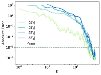
(a) TFIM MODMD Convergence

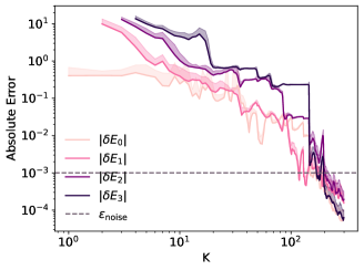
(b) LiH MODMD Convergence

Figure 6: Convergence of eigenenergies for TFIM and LiH. To obtain eigenenergy estimates $\tilde{E}_{n}$, we fix the MODMD parameters $\frac{K}{d}=\frac{5}{2}$ and $\tilde{\delta}=10^{-2}$ for constructing and thresholding the data matrix pair $\mathbf{X},\mathbf{X}^{\prime}\in\mathbb{R}^{dI\times(K+1)}$. Gaussian $\mathcal{N}(0,\varepsilon_{\rm noise}^{2})$ noise with $\varepsilon_{\rm noise}=10^{-3}$ is added independently to distinct matrix elements. The absolute errors, $\lvert\tilde{E}_{n}-E_{n}\rvert$, in the first four lowest target eigenenergies of the TFIM and LiH Hamiltonians are shown with respect to $K$ proportional to the non-dimensional maximal simulation time. The reference states $\ket{\phi_{0}}$ are sparse in the computational basis as prescribed in Section E.1. The shading above the solid lines indicates standard deviation across repeated trials for each quantity. Left TFIM absolute errors from the MODMD algorithm with $\Delta t\approx 0.08$ and $I=6$ (plotted on a log-log scale), where the convergence results are averaged over 20 trials, each involving a Gaussian noise realization and a random selection of $I$ observables. Right. LiH absolute errors from the MODMD algorithm with $\Delta t\approx 0.33$ and $I=6$ (on a log-log scale), where the results are averaged over 20 trials, each involving a Gaussian noise realization.