Measurement of the Higgs boson mass and width using the four-lepton final state in proton-proton collisions at $\sqrt{s}=13\TeV$

Abstract

A measurement of the Higgs boson mass and width via its decay to two bosons is presented. Proton-proton collision data collected by the CMS experiment, corresponding to an integrated luminosity of 138at a center-of-mass energy of 13is used. The invariant mass distribution of four leptons in the on-shell Higgs boson decay is used to measure its mass and contrain its width. This yields the most precise single measurement of the Higgs boson mass to date, $125.04\pm 0.12\GeV$, and an upper limit on the width $\Gamma_{\PH}<330\MeV$ at 95% confidence level. A combination of the on- and off-shell Higgs boson production decaying to four leptons is used to determine the Higgs boson width, assuming that no new virtual particles affect the production, a premise that is tested by adding new heavy particles in the gluon fusion loop model. This result is combined with a previous CMS analysis of the off-shell Higgs boson production with decay to two leptons and two neutrinos, giving a measured Higgs boson width of $3.0^{+2.0}_{-1.5}\MeV$, in agreement with the standard model prediction of 4.1. The strength of the off-shell Higgs boson production is also reported. The scenario of no off-shell Higgs boson production is excluded at a confidence level corresponding to 3.8 standard deviations.

0.1 Introduction

The standard model (SM) of particle physics postulates the existence of a Higgs field responsible for the generation of the masses of fundamental particles. The excitation of this field is known as the Higgs boson ($\PH$) [StandardModel67_1, Englert:1964et, Higgs:1964ia, Higgs:1964pj, Guralnik:1964eu, StandardModel67_2, StandardModel67_3]. The properties of the Higgs boson, observed with a mass of approximately 125by the ATLAS and CMS Collaborations [Aad:2012tfa, Chatrchyan:2012xdj, Chatrchyan:2013lba] at the CERN LHC, are found to be consistent with the expectations of the SM [ATLASnature, CMSnature]. The mass of the Higgs boson ($m_{\PH}$) is a free parameter of the model and, since it determines all other Higgs properties, should be measured with as high precision as possible. For example, the Higgs boson couplings to vector bosons strongly depend on the Higgs boson mass and are precisely predicted by the SM. Another important Higgs boson characteristic is its lifetime, predicted by the SM to be $1.6\times 10^{-22}$ s, corresponding to a total width ($\Gamma_{\PH}$) of $4.1$ [deFlorian:2016spz], as predicted precisely within the SM for $m_{\PH}=125\GeV$. A deviation from the SM prediction would point to either anomalous Higgs boson couplings or its decay to yet undiscovered particles.

The ATLAS and CMS Collaborations measured the Higgs boson mass to be $125.09\pm 0.24\GeV$ [Aad:2015zhl] using $\sqrt{s}=7$ and 8proton-proton ($\Pp\Pp$) collision data from the 2011–2012 data-taking periods (Run 1), corresponding to a total integreted luminosity per experiment of 25. This result has been superseded by both collaborations. The ATLAS experiment measured the Higgs boson mass to be $125.11\pm 0.11(\pm 0.09)\GeV$ [ATLAS_mass], combining the $\PH\to\PGg\PGg$ and $\PH\to 4\Pell$ ($\Pell=\Pe$, $\PGm$) channels from Run 1 and data collected at $\sqrt{s}=13\TeV$ in 2015–2018 (Run 2). The value in parentheses is the statistical uncertainty only. The most recent CMS result, also using the $\PH\to\PGg\PGg$ and $\PH\to 4\Pell$ channels and including Run 1 and 36of $\sqrt{s}=13\TeV$ data from 2016, is $m_{\PH}$ = $125.38\pm 0.14$ $(\pm 0.11)\GeV$. Measurements from ATLAS and CMS using only the $\PH\to 4\Pell$ channel and 2016 data are $124.94\pm 0.18(\pm 0.17)\GeV$ and $125.26\pm 0.21(\pm 0.19)\GeV$, respectively.

Considering only on-shell Higgs boson production, CMS set an upper limit on the Higgs boson width $\Gamma_{\PH}<1.10\GeV$ at 95% confidence level (), limited by the four-lepton invariant mass resolution [Khachatryan:2014jba, Sirunyan:2017exp]. Both the ATLAS and CMS experiments have also set limits on $\Gamma_{\PH}$ [Khachatryan:2014iha, Aad:2015xua, Khachatryan:2015mma, Khachatryan:2016ctc, Aaboud:2018puo, Sirunyan:2019twz, CMS:2022ley] from an off-shell production method [Caola:2013yja, Kauer:2012hd, Campbell:2013una], which relies on the measurement of the ratio of off- to on-shell production rates. Considering both gluon fusion ($\Pg\Pg\PH$) and electroweak (EW) processes, the most recent measurements are $\Gamma_{\PH}=3.2^{+2.4}_{-1.7}\MeV$ [CMS:2022ley] and $\Gamma_{\PH}=4.3^{+3.3}_{-2.5}\MeV$ [atlascollaboration2023evidence] by CMS and ATLAS, respectively. Finally, from an upper limit on the Higgs boson flight distance in the detector, CMS set a lower limit of $\Gamma_{\PH}>3.5\times 10^{-9}$at 95%  [Khachatryan:2015mma].

This paper reports an updated CMS measurement of the Higgs boson mass and width using on-shell production and the $\PH\to 4\Pell$ decay. The data sample includes 138of $\Pp\Pp$ collision data at $\sqrt{s}=13\TeV$ collected in 2016–2018, in combination with the Run 1 data. Compared to the previous CMS on-shell Higgs boson measurement in this channel [Sirunyan:2017exp], the statistical and systematic uncertainties affecting $m_{\PH}$ have been reduced by including the beam spot in a refit of the muon tracks; adopting an improved event categorization procedure; and performing a detailed study of the lepton momentum scale and resolution.

A measurement of the relative off- and on-shell Higgs boson production offers direct information about $\Gamma_{\PH}$ [Caola:2013yja, Kauer:2012hd, Campbell:2013una]. For each Higgs boson production mechanism $j$, with subsequent decay to four leptons, the on- and off-shell cross sections $\sigma_{j}$ are proportional to

$$\sigma_{j}^{\text{on-shell}}\propto\mu_{j}^{\text{on-shell}}\quad\text{and}\quad\sigma_{j}^{\text{off-shell}}\propto\mu_{j}^{\text{on-shell}}\ \Gamma_{\PH},$$ (1)

where $\mu_{j}^{\text{on-shell}}$ is the on-shell signal strength, defined as the ratio of the observed number of on-shell four-lepton events relative to the SM expectation. The signal strength is denoted as $\mu_{\cmsSymbolFace{F}}$ for Higgs boson production mechanisms driven by fermion couplings, , production via $\Pg\Pg\PH$ or in association with a ($\PQt\PAQt\PH$) or $\PQb\PAQb$ pair ($\PQb\PAQb\PH$). For EW production, , production via vector boson fusion ($\mathrm{VBF}$) or in association with a $\PW$ or $\PZ$ boson ($\PV\PH$), the ratio is denoted as $\mu_{\PV}$. Contrary to on-shell in both gluon fusion and EW production, there is sizable destructive interference between the Higgs boson signal and the nonresonant four-lepton production in the off-shell region [Lee:1977yc, Kauer:2012hd]. This interference is crucial for maintaining unitarity and scales with $\sqrt{\smash[b]{\mu_{j}^{\text{on-shell}}\Gamma_{\PH}}}$.

In the described technique for measuring $\Gamma_{\PH}$, it is anticipated that the ratio of the couplings governing off- and on-shell production production matches the SM prediction. In particular, it is assumed that the dominant production mechanism is $\Pg\Pg\PH$ rather than quark-antiquark annihilation. The dominance of the $\Pg\Pg\PH$ production mechanism has been thoroughly tested in the on-shell regime [deFlorian:2016spz, CMSnature]. It is also assumed that beyond-SM particles do not make significant contributions to the $\Pg\Pg\PH$ loop within the mass range considered by the analysis. In this paper, we explicitly test this assumption for the first time through a joint off- and on-shell analysis and find that the $\Gamma_{\PH}$ constraints are not substantially altered. In our previous off-shell analyses [Sirunyan:2019twz, CMS:2022ley], we evaluated the anomalous contributions to the $\PH\PV\PV$ vertex (where $\PV$ denotes a boson, boson, or $\PGg$) in both EW production and Higgs boson decay. We found that these potential contributions did not significantly affect the $\Gamma_{\PH}$ bounds. It is also assumed that no beyond-SM particles, such as higher-mass resonances, significantly contribute within the mass range investigated by the analysis. However, such resonances would typically increase the yield of events at higher masses, which is not supported by our measurement, and no such resonances have been found in a direct search [Sirunyan:2018qlb]. These tests do not address every possible scenario that could impact the measurement of the width, but a violation of any of the above assumptions would, by itself, indicate the presence of physics beyond the SM.

The Higgs boson width may deviate from the SM expectation of 4.1 [deFlorian:2016spz] if the Higgs boson has non-SM decay channels, or if the known decay modes have non-SM rates. Therefore, the direct measurement of the Higgs boson width complements searches for Higgs boson decays to invisible or undetected particles and measurements of the Higgs boson couplings to the known SM particles. For example, if the Higgs boson decays into a pair of unknown particles, potentially candidates for dark matter, this would increase the predicted Higgs boson width but would not introduce a bias into the measurement technique.

0.2 The CMS detector

The central feature of the CMS apparatus is a superconducting solenoid of 6m internal diameter, providing a magnetic field of 3.8T. Within the solenoid volume are a silicon pixel and strip tracker, a lead tungstate crystal electromagnetic calorimeter (ECAL), and a brass and scintillator hadron calorimeter (HCAL), each composed of a barrel and two endcap sections. Forward calorimeters extend the pseudorapidity coverage provided by the barrel and endcap detectors. Muons are reconstructed in gas-ionization detectors embedded in the steel flux-return yoke outside the solenoid. More detailed descriptions of the CMS detector, together with a definition of the coordinate system used and the relevant kinematic variables, can be found in Refs. [CMS:2008xjf, CMS:2023gfb].

Events of interest are selected using a two-tiered trigger system. The first level, composed of custom hardware processors, uses information from the calorimeters and muon detectors to select events at a rate of around 100kHz within a fixed latency of about 4 [Sirunyan:2020zal]. The second level, known as the high-level trigger, consists of a farm of processors running a version of the full event reconstruction software optimized for fast processing, and reduces the event rate to around 1kHz before data storage [Khachatryan:2016bia].

The primary vertex is taken to be the vertex corresponding to the hardest scattering in the event, evaluated using tracking information alone, as described in Section 9.4.1 of Ref. [CMS-TDR-15-02].

The electron momentum is estimated by combining the energy measurement in the ECAL with the momentum measurement in the silicon tracker. The transerve momentum () resolution for electrons with $\pt\approx 45\GeV$ from $\PZ\to\Pe\Pe$ decays ranges from 1.6 to 5%. It is generally better in the barrel region than in the endcaps, and also depends on the bremsstrahlung energy emitted by an electron as it traverses the material in front of the ECAL [eleReco, ScaleSmear2].

Muons are measured in the pseudorapidity range $\abs{\eta}<2.4$, with detection planes made using three technologies: drift tubes, cathode strip chambers, and resistive plate chambers. The single-muon trigger efficiency exceeds 90% over the full $\eta$ range, and the efficiency to reconstruct and identify muons is greater than 96%. Matching muons to tracks measured in the silicon tracker results in a relative transverse momentum resolution, for muons with up to 100, of 1% in the barrel and 3% in the endcaps. The resolution in the barrel is better than 7% for muons with up to 1 [MuReco].

0.3 Data and simulated samples

The data sample used in this analysis corresponds to integrated luminosities of 36.3, 41.5, and 59.8collected in 2016, 2017, and 2018, respectively, for a total of 138at a center-of-mass energy of 13. Events are selected online using the same set of triggers as adopted in Ref. [Sirunyan:2021rug]. They require the presence of at least one lepton (either muon or electron), or up to three leptons with relaxed conditions. The trigger efficiency relative to the offline selection is found to be larger than 99%, measured in data using $4\Pell$ events collected by the single-lepton triggers. It agrees with the expectation from simulation at permille precision. Monte Carlo simulations are used to model signal processes, which involve the Higgs boson and background processes.

On-shell Higgs boson production through $\Pg\Pg\PH$ is simulated using the  2.0 [Frixione:2007vw, Bagnaschi:2011tu, Nason:2009ai, Luisoni:2013kna, Hartanto:2015uka, PowhegBox_1, PowhegBox_2] event generator at next-to-leading order (NLO) in quantum chromodynamics (QCD). Simulation with the MINLO [Hamilton:2012np] program at NLO in QCD is used for the evaluation of systematic uncertainties related to the modeling of jets produced in association with the Higgs boson. Modeling of associated jet activity in gluon fusion simulation is important for categorization of events across a wide range of four-lepton invariant masses for the Higgs boson off-shell analysis.

On-shell Higgs boson production through $\mathrm{VBF}$, in association with a $\PW$ or $\PZ$ boson, or with a pair, is simulated using both  2.0 at NLO in QCD and JHUGen 7.3.0 [Gao:2010qx, Bolognesi:2012mm, Anderson:2013afp, Gritsan:2016hjl, Gritsan:2020pib] at leading order (LO) in QCD. Production in association with a $\PQb\PAQb$ pair or a single top quark is simulated only at LO in QCD with JHUGen. In the $\mathrm{VBF}$, $\PV\PH$, and $\PQt\PAQt\PH$ production modes, the JHUGen and simulations are explicitly compared after parton showering, and no significant differences are found in the kinematic observables. Both on- and off-shell Higgs boson production are simulated following Refs. [Sirunyan:2019twz, CMS:2022ley]. Therefore, the JHUGen simulation is adopted to describe kinematic distributions in the $\mathrm{VBF}$, $\PV\PH$, $\PQt\PAQt\PH$, $\PQb\PAQb\PH$, and $\PQt\PQq\PH$ production mechanisms in the on-shell region, with the expected yields taken from the higher-order simulation. The considered $\PV\PH$ process does not include $\Pg\Pg\to\PZ\PH$ production, which is expected to contribute only about 5% of the $\PV\PH$ cross section [deFlorian:2016spz], and is therefore neglected in this analysis.

The samples modeling off-shell production include interference effects between diagrams with and without the Higgs boson in the propagator. The $\Pg\Pg\to\PZ\PZ$ / $\PZ\PGg^{*}\to 4\Pell$ process is simulated with  7.0.1 [MCFM, Campbell:2011bn, Campbell:2013una, Campbell:2015vwa], which is integrated into the JHUGen generator framework, which is also used to model the vector boson scattering and triple-gauge-boson ($\cmsSymbolFace{VVV}$) backgrounds, the EW signal, and their interference. The background is modeled using the matrix elements. The JHUGen framework enables the incorporation of anomalous interactions involving the Higgs boson or gauge bosons in both $\Pg\Pg\PH$ and EW production processes. The simulation of the EW processes is validated by comparing its results to those obtained with the phantom 1.3 generator [Ballestrero:2007]. All off-shell production simulations are conducted at LO in QCD, with higher-order corrections included through a $K$ factor, as described later.

The mela [Gao:2010qx, Bolognesi:2012mm, Anderson:2013afp, Gritsan:2016hjl, Gritsan:2020pib] package contains a library of matrix elements from JHUGen for the simulation of the signal channel and from for the background, which enables further reweighting of the generated off-shell samples, as discussed in the following. The program is used to simulate wide resonances with masses ranging from 115to 3produced in $\Pg\Pg\PH$, $\mathrm{VBF}$, or $\PV\PH$, and the JHUGen program simulates their decay to four leptons. The events from the $\POWHEG+\textsc{JHUGen}$ simulation are reweighted using the mela package to model off-shell Higgs boson production distributions, as an alternative approach to the direct off-shell simulation discussed above. The two approaches are complementary and allow us to apply mutual cross-checks. Both approaches use the same LO matrix elements available in the mela package based on the JHUGen framework. Reweighting of simulated high-mass $\POWHEG+\textsc{JHUGen}$ events allows the modeling to start from NLO calculations of the SM signal hard-scattering production integrated with the parton shower simulation, compared to integrating LO production of direct off-shell samples. This gives better modeling of the associated jet activity in the events. Furthermore, introducing additional reweighting based on the LO matrix elements would lead to more complexity and internal inconsistencies in the QCD order, which is utilized in the reweighting to obtain both the background and interference predictions.

In the gluon fusion process, the factorization and renormalization scales are allowed to run by equating them to $m_{4\Pell}/2$. To include higher-order QCD corrections, signal cross section calculations are performed at LO, NLO, and next-to-NLO (NNLO), using the and hnnlo 2 programs [Catani:2007vq, Grazzini:2008tf, Grazzini:2013mca] with a narrow-width approximation, for a wide range of masses covering both on- and off-shell ranges. The ratios between the NNLO and LO cross section values, called the NNLO-to-LO $K$ factors, are used to reweight [deFlorian:2016spz] the $m_{4\Pell}$ distributions from the and JHUGen simulations at LO in QCD. A uniform $K$ factor of 1.10 is applied across the entire $m_{4\Pell}$ range to normalize the Higgs boson production cross section via gluon fusion to the predictions for $m_{4\Pell}\approx 125\GeV$ at next-to-NNLO (N${}^{3}\text{LO}$) in QCD [deFlorian:2016spz]. The $m_{4\Pell}$ distributions obtained from the $\POWHEG+\textsc{JHUGen}$ simulation of the $\Pg\Pg\PH$ process are reweighted with the NNLO-to-NLO $K$ factors.

While the NNLO-to-LO $K$ factor calculation is directly applicable to the signal cross section, it is only approximate for the $\Pg\Pg\to\PZ\PZ$ background and its interference with the signal. An approximate NLO calculation  [Caola:2015psa, Melnikov:2015laa, Campbell:2016ivq, Caola:2016trd] is available for the background and the interference. Using the results of this NLO calculation instead of the values from the simulation programs leads to an increase in the NNLO-to-NLO K factor for the interference close to the $m_{4\Pell}$ value corresponding to the kinematic threshold for two on-shell bosons. However, the NNLO-to-NLO $K$ factors for the background and interference are consistent with that for the signal within approximately 10% in the relevant mass range for this analysis of $m_{4\Pell}>220\GeV$. We therefore multiply the background and interference contributions by the same NNLO-to-LO $K$ factor and uniform N${}^{3}\text{LO}$ correction, both calculated for the signal and including associated uncertainties. We introduce an additional 10% uncertainty associated with this factor for the background and the square root of this value for the interference.

The $\qqbar\to 4\Pell$ background simulation is performed at NLO in QCD and LO in the EW theory with . The fully differential cross section for this process has been computed at NNLO in QCD [Grazzini:2015hta], and the NNLO-to-NLO $K$ factor as a function of $m_{4\Pell}$ has been applied to the sample. This $K$ factor is 1.1 at $m_{4\Pell}=125\GeV$ and it varies from 1.0 to 1.2 in the $m_{4\Pell}<500\GeV$ range. The uncertainty due to missing EW corrections in the region $m_{4\Pell}<2m_{\PZ}$ is expected to be small compared to the uncertainties in the QCD calculation. An EW NLO-to-LO $K$ factor [Bierweiler:2013dja] is applied to two on-shell bosons. This $K$ factor depends on $m_{4\Pell}$, decreasing from unity (close to 125) to ${\approx}$0.9 (in the $m_{4\Pell}>500\GeV$ range). The uncertainty in the latter is the dominant uncertainty for the off-shell width measurement and is applied as a function of $m_{4\Pell}$. In the on-shell region, the EW background from the $\PV\PV\PV$, $\ttbar\PV\PV$, and $\ttbar\PV$ processes is generated with  [Alwall:2014hca].

All signal and background event generators are interfaced with the  8.320 program [Sjostrand:2014zea] to simulate multiparton interactions, parton showering, and hadronization. The CUETP8M1 and CP5 tunes [Khachatryan:2015pea, Sirunyan:2019dfx] are applied in simulating the 2016 and 2017–2018 data-taking periods, respectively. The NNPDF 3.1 parton distribution functions [Ball:2011uy] are used for all simulated samples. Simulated events include the contribution from additional $\Pp\Pp$ interactions within the same or adjacent bunch crossings (pileup) and are weighted to reproduce the pileup distribution observed in data. The generated events are further processed through a detailed simulation of the CMS detector based on  [Agostinelli2003250].

0.4 Event reconstruction and selection

The event reconstruction is based on the particle-flow (PF) algorithm [Sirunyan:2017ulk]. This algorithm aims to reconstruct and identify each individual particle in an event, with an optimized combination of information from the various elements of the CMS detector. The energy of photons is obtained from the ECAL measurement. The energy of electrons is determined from a combination of the electron momentum at the primary vertex as determined by the tracker, the energy of the corresponding ECAL cluster, and the energy sum of all bremsstrahlung photons spatially compatible with originating from the electron track. The energy of muons is obtained from the curvature of the corresponding track. The energy of charged hadrons is determined from a combination of their momentum measured in the tracker and the matching ECAL and HCAL energy deposits, corrected for the response function of the calorimeters to hadronic showers. Finally, the energy of neutral hadrons is obtained from the corresponding corrected ECAL and HCAL energies.

Muons with $\pt>5\GeV$ are reconstructed within the geometrical acceptance, corresponding to the region $\abs{\eta}<2.4$, by combining information from the silicon tracker and the muon systems [MuReco]. The muons are selected among the reconstructed muon track candidates by applying quality requirements on the track in both the muon and silicon tracker systems, and demanding small energy deposits in the calorimeters. A relative muon isolation variable is defined as

$${\mathcal{I}}^{\PGm}\equiv\Big{(}\sum\pt^{\text{charged}}+\max\big{[}0,\sum\pt^{\text{neutral}}+\sum\pt^{\PGg}-\pt^{\mathrm{PU}}\big{]}\Big{)}/\pt,$$ (2)

where $\pt$ is the muon transverse momentum, and $\pt^{\text{charged}}$, $\pt^{\text{neutral}}$, and $\pt^{\PGg}$ are the transverse momentum of charged hadrons, neutral hadrons, and photons, respectively, within an cone radius of $\Delta R=0.3$ around the muon direction at the primary vertex.
Here, $\Delta R(i,j)\equiv\sqrt{\smash[b]{(\eta^{i}-\eta^{j})^{2}+(\phi^{i}-\phi^{j})^{2}}}$, where $\phi$ is the azimuthal angle, and in this case i refers to the hadron or photon, and j to the muon. Since the isolation variable is particularly sensitive to energy deposits from pileup interactions, a contribution $\pt^{\mathrm{PU}}$ from pileup is subtracted from the isolation parameter, as shown in Eq. (2). It is defined as the sum of all charged hadrons $i$ not originating from the primary vertex $\pt^{\mathrm{PU}}=0.5\sum_{i}\pt^{i,\mathrm{PU}}$, where the 0.5 factor accounts for the different fraction of charged and neutral hadrons [PUmitigationCMS]. A requirement of ${\mathcal{I}^{\PGm}}<0.35$ is placed on each muon in the event.

Photons from final-state radiation are reconstructed using the PF algorithm [Sirunyan:2017ulk]. Isolated photons with $\pt>2\GeV$, $\abs{\eta}<2.4$, and $\mathcal{I}^{\PGg}<1.8$, are associated with the closest lepton (either muon or electron) in the event. Photons that do not satisfy the requirements $\Delta R(\PGg,\Pell)/(\pt^{\PGg})^{2}<0.012\GeV^{-2}$ and $\Delta R(\PGg,\Pell)<0.5$ are discarded. If more than one photon candidate fulfils the above conditions, the one with the lowest value of $\Delta R(\PGg,\Pell)/(\pt^{\PGg})^{2}$ with respect to the given lepton is retained. Photons passing the above criteria are excluded from the computation of the relative isolation parameter.

Electrons with $\pt>7\GeV$ are reconstructed within the geometrical acceptance, corresponding to the pseudorapidity region $\abs{\eta}<2.5$ [eleReco]. They are identified using a multivariate discriminant, which includes observables sensitive to the emission of bremsstrahlung along the electron trajectory, the geometrical and momentum-energy matching between the electron trajectory and the associated cluster in the ECAL, the shape of the electromagnetic shower in the ECAL, and variables that discriminate against electrons originating from photon conversions. The isolation parameter sums for electrons, defined similarly as for muons, are included in the multivariate discriminant. This information is used to discriminate between prompt leptons from boson decays and those arising from EW decays of hadrons within jets. The package XGBoost [xgboost] is used to train and optimize this multivariate discriminant. The training is performed with simulated events that are not used at any other stage of the analysis. Separate trainings are performed for the three different data-taking periods [ElectronBDT]. Electrons from photon conversions and muons from in-flight decays of hadrons are rejected if the ratio of their impact parameter in three dimensions, computed with respect to the primary vertex position, to their uncertainty is greater than four.

The reconstruction and selection efficiencies for prompt leptons in both data and simulation have been estimated using a tag-and-probe technique [CMS:2011aa] based on samples of $\PZ$ boson events. The ratio of the efficiencies measured in data and simulation is used to rescale the yields of selected events in the simulated samples. In addition, $\PZ$ boson events have been used to calibrate the momentum scale and resolution of electrons and muons in bins of different kinematic variables [ScaleSmear2, Roch2].

In the selection of Higgs boson candidates, four prompt and isolated leptons are required following the prescription above. One of the leptons must have $>20$and at least one of the remaining leptons satisfy $\pt>10\GeV$. The boson candidates are constructed from $\Pep\Pem$ or $\PGmp\PGmm$ pairs whose invariant mass is in the range 12–120. The dilepton pairs are then combined to form the Higgs boson candidate. In the following, $\PZ_{1}$ denotes the pair with the mass closest to the nominal $\PZ$ boson mass, while $\PZ_{2}$ refers to the remaining one. Four possible combinations are considered and treated separately: 4, 4, $2\Pe 2\PGm$, and $2\PGm 2\Pe$, where the mixed-flavor final states are separated based on the decay of $\PZ_{1}$. The four possible combinations have different four-lepton mass resolutions (largely driven by whether the $\PZ_{1}$ is formed from 2$\PGm$ or 2$\Pe$) and different amounts of reducible background (largely driven by whether the $\PZ_{2}$ decays to 2or 2). None of the above differences between the flavor channels affect the off-shell Higgs boson analysis and therefore all flavor channels are combined in that measurement. Signal candidates must satisfy $m_{4\Pell}>70$. If more than one Higgs boson candidate can be formed in the event, the one with the highest value of the kinematic discriminant $\mathcal{D}_{\text{bkg}}^{\text{kin}}$, defined in Section 0.6, is retained, unless these candidates consist of the same four leptons. In this case, the candidate with the $\PZ_{1}$ invariant mass closest to the nominal boson mass is retained.

In the off-shell analysis, events are further categorized based on the jets associated with the Higgs boson candidate. The jets are clustered using the anti-jet finding algorithm [Cacciari:2008gp, Cacciari:2011ma] with a distance parameter of 0.4. The jet momentum is determined as the vector sum of all particle momenta in the jet. Jets must satisfy $\pt>30\GeV$ and $\abs{\eta}<4.7$ and must be separated from all selected lepton candidates and any selected final-state radiation photons by demanding $\Delta R(\Pell/\cPgg,{\text{jet}})>0.4$. Jets originating from the hadronization of quarks are identified using the DeepCSV algorithm [Sirunyan:2017ezt], which combines information on impact parameter significance, the secondary vertex, and jet kinematic variables. The use of this identification is described in Section 0.6.

0.5 Lepton momentum measurement and four-lepton mass resolution

Once an event is selected in the Higgs boson mass and on-shell width measurements, beam spot information is used to improve the $m_{4\Pell}$ resolution. In this approach (denoted as BS in the following), the beam spot position is included as a common point in the reconstruction of the tracks from the Higgs boson decay. While muon kinematic parameters such as are recalculated after implementing this constraint, electron kinematic parameters are not modified. This is because the electron momentum is determined mostly by the energy measurement in the ECAL, rather than from the track curvature. Thus, applying the beam spot constraint does not change the momentum measurement. In the final states involving muons, the BS constraint improves the $m_{4\Pell}$ resolution by about 3–8%, mostly depending on the flavor of the leptons originating from $\PZ_{1}$.

Once the BS approach is applied, an important variable, the event-by-event four-lepton mass uncertainty ($\delta m_{4\Pell}$), is introduced. Individual lepton momentum uncertainty (per-lepton uncertainty in the following) is obtained from the algorithms used to estimate lepton momenta. For muons, the full covariance matrix is obtained from the muon track fit, and the uncertainty in the muon direction is assumed to be negligible. For the electrons, the momentum uncertainty is estimated from the combination of the ECAL and silicon tracker measurements, neglecting the uncertainty in the track direction. The per-lepton momentum uncertainty is then propagated to the $m_{4\Pell}$ to predict $\delta m_{4\Pell}$. Each $\delta m_{4\Pell}^{i}$ corresponding to individual lepton momentum variation is calculated separately. The total per-event uncertainty $\delta m_{4\Pell}$ is obtained as the quadrature sum of the four individual $\delta m_{4\Pell}^{i}$.

This invariant mass uncertainty is decreased by applying correcting factors to the momentum uncertainty. These corrections are derived for muons in several $\abs{\eta}$ bins, and for electrons in bins of $\delta$/vs. $\abs{\eta}$. The $2\Pell$ invariant mass distribution is used to extract these corrections. The mass distribution is fit in two steps with a convolution of a Breit–Wigner function (that describes the intrinsic shape of the boson resonance) with a double-sided Crystal Ball function [Skwarnicki:1986xj] (to describe the detector effects), plus an exponential function (used to describe the background). The first step is used to estimate all the parameters in the fit function, while the correction to the momentum uncertainty is determined in the second step. After the corrections are extracted, a closure test between the predicted and measured invariant mass resolutions is performed.

To further improve the $m_{4\Pell}$ resolution, a kinematic fit is also performed using a mass constraint on the intermediate on-shell resonance, with an approach similar to the one described in Ref. [Sirunyan:2017exp]. For a 125 Higgs boson, the selected $Z_{1}$ is mostly on-shell, while the $m_{\PZ_{2}}$ invariant mass distribution is broad and the width is much larger than the detector resolution. When considering the Higgs boson mass measurement, the expected gain in resolution comes from refitting $Z_{1}$. Thus, it is possible to reevaluate the of the two leptons forming $\PZ_{1}$, using the constraint that the reconstructed invariant mass of the boson candidates must follow the true shape of the boson. In every event, the lepton momenta are adjusted using the likelihood function

$$\mathcal{L}(\pt^{1},\pt^{2}|\pt^{\text{reco1}},\sigma^{1},\pt^{\text{reco2}},\sigma^{2})=\text{Gauss}(\pt^{\text{reco1}}|\pt^{1},\sigma^{1})\text{Gauss}(\pt^{\text{reco2}}|\pt^{2},\sigma^{2})\mathcal{L}(m_{12}|m_{\PZ},m_{\PH}),$$

where $\pt^{\text{reco1}}$ and $\pt^{\text{reco2}}$ are the reconstructed transverse momenta of the two leptons forming the $Z_{1}$, $\sigma^{1}$ and $\sigma^{2}$ are the per-lepton resolutions (uncertainties in the measurements, corrected using the method described above), $\pt^{1}$ and $\pt^{2}$ are the observables under optimization, and $m_{12}$ is the invariant mass calculated from $\pt^{1}$ and $\pt^{2}$. Finally, $\mathcal{L}(m_{12}|m_{\PZ},m_{\PH})$ is the likelihood function given the true shapes of $m_{\PZ_{1}}$ and of the 125Higgs boson. For each event, the likelihood is maximized and the values of the refitted leptons are updated.

For the Higgs boson off-shell production, the $m_{4\Pell}$ distribution is much broader than the $m_{4\Pell}$ resolution, and, therefore, improvements in the treatment of the lepton momentum uncertainties are not applied. Figure 1 shows the $m_{4\Pell}$ distribution inclusively for all the four-lepton states (upper plot) and separately for the four individual final states. Expectations for the signal and background contributions are shown as stacked histograms. The yields from the signal and $\PZ\PZ$ backgrounds are estimated from simulation assuming SM cross sections, while the $\PZ+\PX$ background yield is estimated from data. More details are given in Sections 0.7 and 0.8. Figure 2 displays the distribution of the relative per-event mass uncertainty of the four-lepton system ($\delta m_{4\Pell}/m_{4\Pell}$) in the inclusive final state with $105<m_{4\Pell}<140\GeV$. This variable is used to categorize events in the on-shell region according to their invariant mass resolution. The categorization is performed by defining nine mutually exclusive bins with an equal number of signal events in each. Since each final state has a different resolution that also varies across data-taking periods, the bin boundaries are determined independently per final state and per data-taking year. Figure 3 plots the observed and predicted yields of four-lepton events as a function of $\delta m_{4\Pell}/m_{4\Pell}$ bin for the $105<m_{4\Pell}<140$invariant mass range. This approach improves the precision of the Higgs boson mass measurement by about 10%.

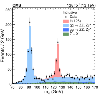
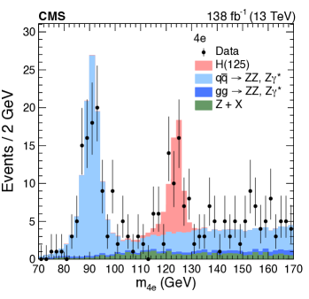
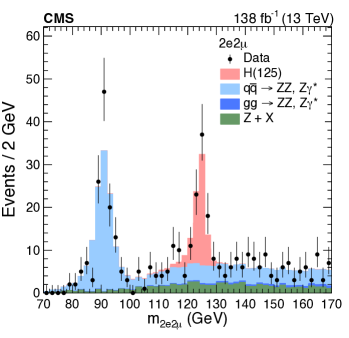
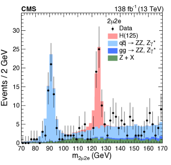
Figure 1: The observed (points) and predicted (stacked histograms) $m_{4\Pell}$ distributions in the inclusive (upper), 4$\PGm$ (middle left), 4$\Pe$ (middle right), 2$\Pe$2$\PGm$ (lower left) and 2$\PGm 2\Pe$ (lower right) final states, defined such that the first lepton pair is taken to be the one with the mass closest to the nominal $\PZ$ boson mass. The predictions for the Higgs boson signal and the three main backgrounds are given by the different colors. The vertical bars on the points show the statistical uncertainties in the data.

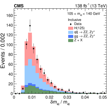
Figure 2: Distributions of the observed (points) and predicted (stacked histograms) relative per-event mass uncertainty of the four-lepton system, in the inclusive final state. The predictions for the Higgs boson signal and the three main backgrounds are given by the different colors. The vertical bars on the points show the statistical uncertainties in the data.

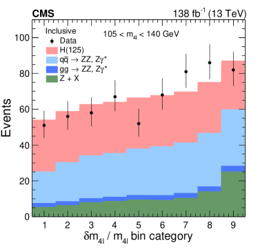
Figure 3: Observed (points) and predicted (stacked histograms) yields of four-lepton events in each of the 9 $\delta m_{4\Pell}/m_{4\Pell}$ bin categories for the inclusive final state. The bins are shown in the order of increasing $\delta m_{4\Pell}/m_{4\Pell}$. The predictions for the Higgs boson signal and the three main backgrounds are given by the different colors. The vertical bars on the points show the statistical uncertainties in the data.

0.6 Kinematic discriminants and off-shell event categorization

The reconstructed four-lepton events and their associated jets, where relevant, can be described with several observables using the kinematic features of the Higgs boson decay and associated particles. It is a challenging task to perform an optimal analysis in a large multidimensional phase space. There are up to 13 observables in the set $\boldsymbol{\Omega}$ that describe the Higgs boson kinematic distributions in the $2\to 6$ process of collision of two protons and the production of four leptons and two associated jets. The mela approach is designed to reduce the number of observables to the minimum while retaining all essential information. In this method, optimal discriminators are defined through the utilization of matrix element likelihood calculations [Gao:2010qx, Bolognesi:2012mm, Anderson:2013afp, Gritsan:2016hjl, Gritsan:2020pib]. Two types of discriminants are defined for each of the Higgs boson production and decay processes as

$$\mathcal{D}_{\text{alt}}\left(\boldsymbol{\Omega}\right)=\frac{\mathcal{P}_{\text{sig}}\left(\boldsymbol{\Omega}\right)}{\mathcal{P}_{\text{sig}}\left(\boldsymbol{\Omega}\right)+\mathcal{P}_{\text{alt}}\left(\boldsymbol{\Omega}\right)}$$ (3)

and

$$\mathcal{D}_{\text{int}}\left(\boldsymbol{\Omega}\right)=\frac{\mathcal{P}_{\text{int}}\left(\boldsymbol{\Omega}\right)}{2\ \sqrt{{\mathcal{P}_{\text{sig}}\left(\boldsymbol{\Omega}\right)\ \mathcal{P}_{\text{alt}}\left(\boldsymbol{\Omega}\right)}}},$$ (4)

where the probability of a certain process $\mathcal{P}$ is calculated using the full set of kinematic observables $\boldsymbol{\Omega}$ for the processes denoted as “sig” for a signal model and “alt” for an alternative model, which can be for either an alternative Higgs boson production mechanism, or a background, depending on the individual case. The “int” label represents the interference between the two model contributions. The probabilities $\mathcal{P}$ are calculated from the matrix elements obtained from the mela approach.

The ${\mathcal{D}}^{\text{kin}}_{\text{bkg}}$ discriminant is used in the selection of events, as discussed in Section 0.4, and as one of the observables in the maximum likelihood fit for the signal extraction, in both the on- and off-shell analyses. It is determined following Eq. (3), where $\mathcal{P}_{\text{bkg}}$ is calculated for the dominant $\qqbar\to 4\Pell$ background process and $\mathcal{P}_{\text{sig}}$ is found for the $\PH\to 4\Pell$ decay using the full kinematic information of the four leptons. Figure 4 shows the inclusive ${\mathcal{D}}^{\text{kin}}_{\text{bkg}}$ distribution of the four-lepton system. The inclusion of ${\mathcal{D}}^{\text{kin}}_{\text{bkg}}$ in the analysis produces a $4\%$ improvement in the $m_{4\Pell}$ resolution. In the off-shell analysis, the ${\mathcal{D}}^{\text{kin}}_{\text{bkg}}$ discriminant is used for events without associated jets.

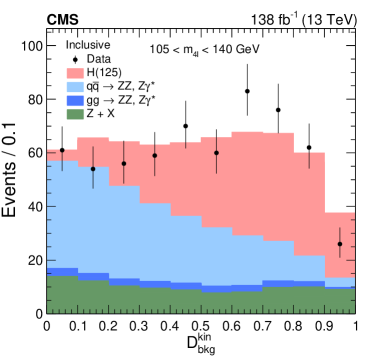
Figure 4: Distributions of the observed (points) and predicted (stacked histograms) ${\mathcal{D}}^{\text{kin}}_{\text{bkg}}$ of the four-lepton system, in the inclusive final state. The predictions for the Higgs boson signal and the three main backgrounds are given by the different colors. The vertical bars on the points show the statistical uncertainties in the data.

For the two categories of off-shell events with two associated jets described below, $\mathrm{VBF}$- and $\PV\PH$-tagged events, $\mathcal{P}_{\text{bkg}}$ and $\mathcal{P}_{\text{sig}}$ include the kinematic information on the four leptons and the two jets. The $\mathcal{P}_{\text{bkg}}$ probability density corresponds to the EW and QCD background processes with four leptons and two jets, while $\mathcal{P}_{\text{sig}}$ is determined for the EW signal processes $\mathrm{VBF}$ and $\PV\PH$. Including jet kinematic information in the ${\mathcal{D}}_{\text{bkg}}$ calculation improves the separation of the signal from both the background and $\Pg\Pg\PH$ production, when compared to ${\mathcal{D}}^{\text{kin}}_{\text{bkg}}$.

In the analysis of the off-shell region, a dedicated study of a particular kinematic topology is done, treating gluon fusion and EW production separately, because they evolve differently with $m_{4\Pell}$, thus allowing us to probe their individual behaviors. Therefore, in the off-shell region, events are further split into three mutually exclusive categories based on the presence of other particles produced in association with the Higgs boson candidate [Sirunyan:2021rug]. This is not necessary in the on-shell analysis.

We use various kinematic discriminants and other selection requirements to perform the categorization of the off-shell events. The definition of these discriminants is given by Eq. (3). They are specifically designed to distinguish the targeted signal production mechanisms ($\mathrm{VBF}$, $\PW\PH$, $\PZ\PH$) within each category from gluon fusion production and are denoted as $\mathcal{D}_{\text{2jet}}^{\mathrm{VBF}}$, $\mathcal{D}_{\text{2jet}}^{\PZ\PH}$, and $\mathcal{D}_{\text{2jet}}^{\PW\PH}$. They are labeled to indicate a specific dijet topology (“2jet”) and production mechanism ($\mathrm{VBF}$, $\PW\PH$, $\PZ\PH$). Calculated using the mela approach with matrix elements at LO in QCD, these discriminants utilize the complete kinematic information from the Higgs boson decay and the associated jets. Additional details can be found in Refs. [Sirunyan:2017exp, Sirunyan:2017tqd, Sirunyan:2019twz, Sirunyan:2021rug].

The selected off-shell events are split into three categories: $\mathrm{VBF}$-tagged, $\PV\PH$-tagged, and Untagged events, as summarized in Table 0.6. The discriminants $\mathcal{D}_{\text{2jet}}$ are constructed following Eq. (3), where $\mathcal{P}_{\text{sig}}$ corresponds to the signal probability for $\mathrm{VBF}$ ($\PW\PH$ or $\PZ\PH$) production in the $\mathrm{VBF}$-tagged ($\PV\PH$-tagged) category, and $\mathcal{P}_{\text{alt}}$ to Higgs boson production via $\Pg\Pg\PH$ in association with two jets. When more than two jets pass the selection criteria, the two jets with the highest are chosen for the matrix element calculations. Thereby, the $\mathcal{D}_{\text{2jet}}$ discriminants separate the targeted signal production mode of each category from $\Pg\Pg\PH$ production using only the kinematic variables of the Higgs boson and the two associated jets. Sequential selection criteria are applied to define the categories as follows:

• The $\mathrm{VBF}$-2jet category requires exactly four leptons. In addition, there must be either two or three jets of which at most one is identified as coming from the hadronization of a quark, which we term a -tagged jet [Sirunyan:2021rug], or at least four jets and no -tagged jets. Finally, $\mathcal{D}_{\text{2jet}}^{\mathrm{VBF}}>0.5$ is required [Sirunyan:2021rug].

• The $\PV\PH$-hadronic category requires exactly four leptons. In addition, there must be either two or three jets, or at least four jets and no -tagged jets. Finally, we demand $\max(\mathcal{D}_{\text{2jet}}^{\PW\PH},~{}\mathcal{D}_{\text{2jet}}^{\PZ\PH})>0.5$ [Sirunyan:2021rug].

• The Untagged category consists of the remaining events.

Table 0.6 provides a summary of the key categorization requirements, with selections applied sequentially from left to right to define the three mutually exclusive categories. All discriminants are calculated with the JHUGen signal and background matrix elements. The $\PV\PH$ interference discriminant in the $\PV\PH$-tagged category is defined as the simple average of the ones corresponding to the $\PZ\PH$ and $\PW\PH$ processes. The use of decay kinematic information is denoted by the label “dec”.

Summary of the three production categories in the off-shell $m_{4\Pell}$ region and the observables used in the fits. lccc Category & VBF-tagged $\PV\PH$-tagged Untagged

Selection $\mathcal{D}_{\text{2jet}}^{\text{VBF}}>0.5$ $\mathcal{D}_{\text{2jet}}^{\Z\PH}$ or $\mathcal{D}_{\text{2jet}}^{\PW\PH}>0.5$ Rest of the events
Observables $m_{4\Pell}$, $\mathcal{D}^{\text{VBF}+\text{dec}}_{\text{bkg}}$, $\mathcal{D}_{\text{bsi}}^{\text{VBF}+\text{dec}}$ $m_{4\Pell}$, $\mathcal{D}^{\PV\PH+\text{dec}}_{\text{bkg}}$, $\mathcal{D}_{\text{bsi}}^{\PV\PH+\text{dec}}$ $m_{4\Pell}$, $\mathcal{D}^{\text{kin}}_{\text{bkg}}$, $\mathcal{D}_{\text{bsi}}^{{\Pg\Pg}+\text{dec}}$

In each category of events, three observables $\vec{x}$ are defined following Eqs. (3) and (4). As summarized in Table 0.6, $\vec{x}=\{m_{4\Pell},{\mathcal{D}}_{\text{bkg}},{\mathcal{D}}_{\text{int}}\}$. The $m_{4\Pell}$ and ${\mathcal{D}}_{\text{bkg}}$ parameters have already been introduced earlier. The third observable, ${\mathcal{D}}_{\text{int}}$ defined in Eq. (4), separates the interference of Higgs boson production (with SM-like couplings) and the background (used as the alternative model). It is called ${\mathcal{D}}_{\text{bsi}}$ for the signal-background interference in the off-shell region. In the Untagged category, decay information is used in the calculation of ${\mathcal{D}}_{\text{int}}$, as indicated with the label “dec”. In the VBF- and VH-tagged categories, production information from the two associated jets is used, along with decay information. Distributions of the observed and expected $\vec{x}$ observables for events in the off-shell region are illustrated in Fig. 5 for each of the three categories. The expected distributions are found using the SM predicted signal and background cross sections.

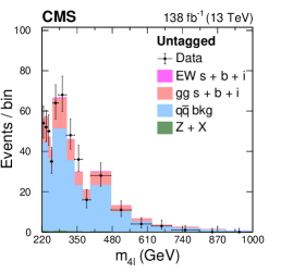
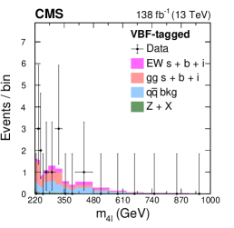
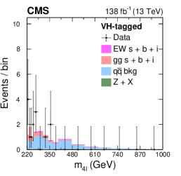
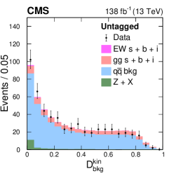
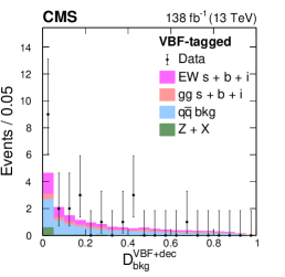
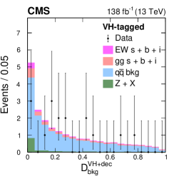
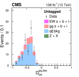
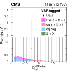
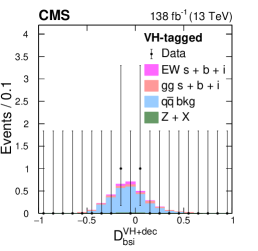
Figure 5: Off-shell data (points) and pre-fit distributions (histograms) for the Untagged (left), $\mathrm{VBF}$-tagged (middle), and $\PV\PH$-tagged (right) categories. The upper row shows $m_{4\Pell}$ distributions with a requirement on ${\mathcal{D}}^{\text{kin}}_{\text{bkg}}>0.6$ (left), $\mathcal{D}^{{\mathrm{VBF}}+{\text{dec}}}_{\text{bkg}}>0.6$ (middle), or $\mathcal{D}^{{\PV\PH}+{\text{dec}}}_{\text{bkg}}>0.6$ (right) applied for illustration purposes to enhance signal over background contributions. The middle row shows $\mathcal{D}^{\text{kin}}_{\text{bkg}}$ (left), $\mathcal{D}^{{\mathrm{VBF}}+{\text{dec}}}_{\text{bkg}}$ (middle), $\mathcal{D}^{{\PV\PH}+{\text{dec}}}_{\text{bkg}}$ (right) distributions, where an additional requirement $m_{4\Pell}>340$is applied to enhance signal-over-background contributions. The lower row plots the $\mathcal{D}_{\text{bsi}}$ with both the $m_{4\Pell}$ and ${\mathcal{D}}^{\text{kin}}_{\text{bkg}}$ requirements specified above. Contributions from the four processes are shown by the different colors, where “s”, “b”, and “i” refer to the signal, background, and interference contributions, respectively. The vertical bars on the points give the statistical uncertainties in the data, and the horizontal bars represent the bin widths. For the prefit distributions, the different cross sections are set to their SM values.

0.7 Estimation of background

The largest background to the Higgs boson signal in the $\PH\to 4\Pell$ channel is from the process $\qqbar\to\PZ\PZ/\PZ\PGg^{*}/\PGg^{*}\PGg^{*}\to 4\Pell$. The $\Pg\Pg\to\PZ\PZ/\PZ\PGg^{*}/\PGg^{*}\PGg^{*}\to 4\Pell$ background process, as well as the EW background, which includes the vector boson scattering and $\PV\PZ\PZ$ processes, interfere with off-shell Higgs boson production and are discussed in more detail in Sections 0.3 and 0.8. The interference between on-shell Higgs boson production and these backgrounds is, instead, negligible. In the on-shell region, the EW background also incorporates other $\PV\PV\PV$, $\ttbar\PV\PV$, and $\ttbar\PV$ processes. To model the $m_{4\Pell}$ distributions for each of these irreducible backgrounds, a Bernstein polynomial of third order is used in the $m_{4\Pell}$ range 105–140 .

An additional background to the Higgs boson signal, referred to as $\PZ+\PX$ in the following, comes from processes in which decays of heavy-flavor hadrons, in-flight decays of light mesons within jets, or charged hadrons overlapping with decays are misidentified as leptons. The main process contributing to this background is $\PZ$+jets production, which is estimated from control regions in data. The control regions are defined by requiring a lepton pair, satisfying all the requirements of a ${\PZ}_{1}$ candidate, along with two additional opposite-sign leptons satisfying looser identification requirements than those in the main analysis. These four leptons are then required to pass the ${\PZ}_{1},{\PZ}_{2}$ selection. The background yield in the signal region is obtained by weighting the control region events by the lepton misidentification probability ($f_{\Pell}$), defined as the fraction of nonsignal leptons that pass the analysis selection criteria. A detailed description of the method can be found in Ref. [Sirunyan:2017exp]. The shape of the $m_{4\Pell}$ distribution from $\PZ+\PX$ events is described by a Landau function. Due to the low number of events, the functional form is extracted using a larger $m_{4\Pell}$ range of 70–770 .

The observed number of data events, expected background, and signal yields are listed in Tables 0.7 and 0.7 for the on- and off-shell region, respectively. The signal and $\PZ\PZ$ background yields are estimated from simulation, while the $\PZ+\PX$ yield is estimated from data. The details of the Higgs boson signal modeling, its interference with background, and the $\PZ\PH$ cross-feed for the off-shell results are given in Section 0.8.

The observed and expected yields for the Higgs boson signal and background contributions in the on-shell region $105<m_{4\Pell}<140\GeV$, for each of the four-lepton categories and the total. lrrrrr 4 4 $2\Pe 2\PGm$ $2\PGm 2\Pe$ Total
Total signal 90.9 48.7 65.5 53.3 258.4
$\qqbar\to 4\Pell$ background 89.2 38.9 64.4 42.1 234.6
$\Pg\Pg\to 4\Pell$ background 9.7 4.9 4.9 3.8 23.4
$\PZ+\PX$ background 32.4 12.2 28.2 18.6 91.3
Total expected 222.2 104.6 163.0 117.8 607.7
Observed 230 94 170 107 601

Table 1: Observed and expected yields for the Higgs boson signal and background contributions in the off-shell region $m_{4\Pell}>220\GeV$, for each of the four-lepton categories and the total. The yields from interference of the signal and background and the $\PZ\PH$ cross-feed are also shown.

lrrrr VBF-tagged VH-tagged Untagged Total
$\Pg\Pg\to 4\Pell$ signal 1.0 0.9 25.1 27.0
$\Pg\Pg\to 4\Pell$ background 16.0 13.5 457.0 486.4
$\Pg\Pg\to 4\Pell$ interference $-2.1$ $-1.9$ $-52.0$ $-56.1$
EW signal 1.3 0.1 1.8 3.2
EW background 14.9 2.9 19.7 37.5
EW interference $-3.4$ $-0.2$ $-3.9$ $-7.4$
$\PZ\PH$ cross-feed 0.2 0.4 7.0 7.6
$\qqbar\to 4\Pell$ background 28.6 46.7 1795.1 1870.4
$\PZ+\PX$ background 4.7 5.3 89.7 99.7
Total expected 61.2 67.8 2339.4 2468.4
Observed 70 67 2335 2472

0.8 Extraction of signal

The modeling of the signal process is different for the on- and off-shell regions. In the on-shell region, there is negligible interference between the Higgs boson and background production, so the signal can be treated separately. At the same time, the narrow Higgs boson peak requires careful treatment of the detector resolution effects. There is also little dependence on the production processes because the $\PH\to 4\Pell$ decay is independent of the production mechanism due to the narrow-width approximation. In the off-shell region, on the other hand, the distributions are much wider, with minimal influence from detector resolution on the measurements. However, there is a sizable interference between the Higgs boson signal and background processes, and their proper treatment requires special care. Moreover, the treatment of the gluon fusion and EW productions is different because of their different evolution with $m_{4\Pell}$.

0.8.1 Signal modeling in the on-shell region

The probability density for the on-shell region includes both signal and background contributions. It is normalized to the total event yield for each process $j$ and category $k$, and can be written as

$$\mathcal{P}_{jk}(\vec{x};\vec{\xi}_{jk},\vec{\zeta})=\mu_{j}\mathcal{P}_{jk}^{\text{sig}}(\vec{x};\vec{\xi}_{jk},\vec{\zeta})+\mathcal{P}_{jk}^{\text{bkg}}(\vec{x};\vec{\xi}_{jk}),$$ (5)

where $\vec{\zeta}$ are the unconstrained parameters of interest, including the signal strength $\mu_{j}$ defined as the ratio of the signal yield to the SM expectation, $\vec{\xi}_{jk}$ are the constrained nuisance parameters for a particular parametrization, and $\vec{x}$ are the observables.

In the on-shell Higgs boson mass and width analysis, there are six signal processes ($\Pg\Pg\PH$, $\mathrm{VBF}$, $\PV\PH$, $\PQt\PAQt\PH$, $\PQb\PAQb\PH$, and $\PQt\PQq\PH$) and three background processes ($\qqbar/\Pg\Pg\to\PZ\PZ/\PZ\PGg^{*}/\PGg^{*}\PGg^{*}\to 4\Pell$ and $\PZ+\PX$). When constraints on $\Gamma_{\PH}$ are determined by simultaneously fitting both the on-shell and off-shell regions, the on-shell region follows Scheme 2 as described in Ref. [CMS:2021nnc], where additional details on categorization and signal and background modeling can be found. Additional details regarding the signal modeling for the mass and width analyses using only the on-shell region are provided below.

For the Higgs boson mass measurement, a one-dimensional (1D) statistical model is built in each category using the observable $m_{4\Pell}$, split between data-taking years and final states, and taking each of the nine $\delta m_{4\Pell}/m_{4\Pell}$ bins separately. The signal shape for each process is obtained from a fit of the simulated $m_{4\Pell}$ distribution, in the range 105–140, using a double-sided Crystal Ball function [Oreglia:1980cs]. In the case of $\PV\PH$ and $\PQt\PAQt\PH$ production, a Landau function is added to include the possible contribution of a lepton from Higgs boson decay being outside the detector acceptance or failing the selection criteria. Five simulated mass points (120, 124, 125, 126, and 130 ) are used to parametrize the $m_{\PH}$ dependence of each shape parameter $p^{i}$ in the Crystal Ball and Landau functions. A set of first-order polynomials with constants $a^{i}$ and $b^{i}$ is fitted simultaneously as functions of $m_{\PH}$:

$$p^{i}=a^{i}+b^{i}(m_{\PH}-125\GeV).$$ (6)

The natural width of the Higgs boson is assumed to be much smaller than the instrumental $m_{4\Pell}$ resolution. For the on-shell width measurement instead, the signal shape is the convolution of a Crystal Ball function with a Breit–Wigner function, to include $\Gamma_{\PH}$ as a parameter in the model. This model is referred to as 1D. If the BS and $m(\PZ_{1})$ constraints are applied, the model is referred to as 1D${}^{{}^{\prime}}_{\text{BS}}$. Figure 6 shows an example of the signal model used in the on-shell analysis and how it varies across the $\delta m_{4\Pell}/m_{4\Pell}$ bins.

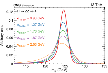
Figure 6: Examples of the on-shell signal model $m_{4\Pell}$ shape for five $\delta m_{4\Pell}/m_{4\Pell}$ bins. For illustration purposes, the mass range shown is reduced to 112–135 , and all final states and all data-taking years are combined. The resolution estimator $\sigma_{i~{}bin}$ is defined as the width of the Gaussian function from a fit to events in bin $i$ having the smallest mass window that contains 68% of the signal events.

This categorization isolates the events with better invariant mass resolution and improves the description of the signal shape and the modeling of the peak position. This latter improvement is most important for the final state where the on-shell boson decays to two electrons. An illustration of the full model used in the on-shell analysis is shown in Fig. 7.

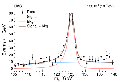
Figure 7: Illustration of how the on-shell statistical model is constructed, combining the $m_{4}\Pell$ distributions from all data-taking years and all final states. The red, blue, and brown lines show the results of the fit to the signal, background, and their sum, respectively.. The solid black points with vertical bars show the data and the associated statistical uncertainties.

Based on the 1D model, a two-dimensional (2D) statistical model is built with a probability density $\mathcal{P}_{\text{2D}}$ using the observables $m_{4\Pell}$ and ${\mathcal{D}}^{\text{kin}}_{\text{bkg}}$ and the expression

$$\mathcal{P}_{\text{2D}}(m_{4\Pell},~{}{\mathcal{D}}^{\text{kin}}_{\text{bkg}})=\mathcal{P}^{\text{sig}}_{\text{1D}}~{}T^{\text{sig}}({\mathcal{D}}^{\text{kin}}_{\text{bkg}}|m_{4\Pell})+\mathcal{P}^{\text{bkg}}_{\text{1D}}~{}T^{\text{bkg}}({\mathcal{D}}^{\text{kin}}_{\text{bkg}}|m_{4\Pell}).$$

The factor $T$, based on a 2D histogram template, is a conditional probability density function of ${\mathcal{D}}^{\text{kin}}_{\text{bkg}}$ and $m_{4\Pell}$, implemented by normalizing the sum of the contents in each $m_{4\Pell}$ histogram bin to one.

The final model, designated $\mathcal{N}$–2D is built by combining all 2D models of $\mathcal{N}$ different $\delta m_{4\Pell}/m_{4\Pell}$ categories. If the BS and $m(\PZ_{1})$ constraint approaches are applied, the model is referred to as $\mathcal{N}$–2$D^{\prime}_{\text{BS}}$. This configuration provides the best Higgs boson mass and width precision and is used as the default for the on-shell measurements. A simultaneous signal-plus-background unbinned fit to all categories is performed to extract $m_{\PH}$ and $\Gamma_{\PH}$. The signal strength is left unconstrained in this fit.

0.8.2 Signal and background interference modeling in the off-shell region

In the off-shell region, the probability density follows Eqs. (1) and (5) closely, with the additional contribution of the interference (“int”) between the signal and background amplitudes, as well as a cross-feed (“cross”) component discussed below. It is parametrized as

$$\mathcal{P}_{jk}(\vec{x};\vec{\xi}_{jk},\vec{\zeta})=\frac{\mu_{j}\Gamma_{\PH}}{\Gamma_{0}}\mathcal{P}_{jk}^{\text{sig}}(\vec{x};\vec{\xi}_{jk})+\sqrt{\frac{\mu_{j}\Gamma_{\PH}}{\Gamma_{0}}}\mathcal{P}_{jk}^{\mathrm{int}}(\vec{x};\vec{\xi}_{jk})+\mu_{j}\mathcal{P}_{jk}^{\text{cross}}(\vec{x};\vec{\xi}_{jk})+\mathcal{P}_{jk}^{\text{bkg}}(\vec{x};\vec{\xi}_{jk}),$$ (7)

where $\Gamma_{0}$ is the reference value of the Higgs boson width (not necessarily its SM value) used in simulation. Otherwise, the definition of the terms is the same as in Eq. (5). In the off-shell width analysis, there are two production modes, $j$ (gluon fusion and EW, which includes both $\mathrm{VBF}$ and $\PV\PH$), and three jet-tagged categories, $k$. All lepton flavors and data periods are combined in this analysis. The contributions from $\PQt\PAQt\PH$, $\PQb\PAQb\PH$, and $\PQt\PQq\PH$ are expected to be negligible in the off-shell region.

The $\mathcal{P}_{jk}^{\text{sig}}$, $\mathcal{P}_{jk}^{\text{int}}$, $\mathcal{P}_{jk}^{\text{cross}}$, and $\mathcal{P}_{jk}^{\text{bkg}}$ probability densities are normalized to the expected number of events, and are implemented as binned histograms (templates) of the observables $\vec{x}$ listed in Table 0.6. These templates are obtained as weighted linear combinations of existing simulated signal or background samples.

The off-shell region includes all events with $m_{4\Pell}$ greater than $220\GeV$. Other processes can mimic off-shell Higgs boson production and decay to four leptons in this region. Specifically, we study on-shell signal events in which the Higgs boson decays to $2\Pell+X$, and $X$ contains further leptons that allow the event to pass the four-lepton selections. The dominant on-shell Higgs boson process that can contaminate the off-shell region is $\PZ(\Pell\Pell)\PH(2\Pell+X)$, called $\PZ\PH$ cross-feed.

The $\PZ\PH$ cross-feed contribution is estimated using on-shell $\PZ\PH$ samples with $\PH\to\PW\PW$ and $\PZ\PZ$ decays, where both hadronic and leptonic decay of the bosons is allowed. The dominant contributions come from the $\PH\to 2\Pell 2\PGn$ and $2\Pell 2\Pq$ final states produced in association with $\PZ\to 2\Pell$. To prevent double counting, on-shell cross-feed events are eliminated from the off-shell simulated samples.

The gluon fusion cross section is calculated using the highest order QCD and EW expansions available to simulate inclusive $\PZ\PZ$ production [deFlorian:2016spz]. However, event categorization depends on modeling associated jets through ’s parton showering and hadronization, which involves matching these processes to the hard-scattering production. Off-shell gluon fusion production is generated at LO with no associated jets at the matrix element level, and therefore all jets come from . The parton showering and hadronization requires setting the hadronization scale, which can depend on the energy scale in the process. In the case of the $\Pg\Pg\to 4\Pell$ process, the energy scale is set at $m_{4\Pell}$.

The EW cross section for the inclusive production of $\PZ\PZ$ and two associated jets is also calculated to the highest order QCD and EW expansion available [deFlorian:2016spz]. Contrary to the gluon fusion process, two hard jets, which are typically the leading jets in the process, are already generated at the matrix element level in the LO simulation. These are the two associated jets in the VBF process, or the two jets from the hadronic decay of the associated or boson. Therefore, the dependence on the parton shower and hadronization and its matching to the hard-scattering production is much weaker for these EW processes.

The categorization efficiency of simulated $\Pg\Pg\PH$ and EW Higgs boson production can be checked using alternative and MINLO simulations. The samples are generated for a wide range of off-shell Higgs boson masses at NLO in QCD, with one jet generated at the matrix element, and using matching to simulate additional jets. The MINLO simulation of $\Pg\Pg\PH$ production is done for Higgs boson masses of 125 and $300\GeV$ at NLO in QCD, with two jets generated at the matrix element level, and matching for additional jets. While the JHUGen categorization efficiencies agree with those using and MINLO within the uncertainties of the QCD scale used in , for the $\Pg\Pg\PH$ process the deviations of the central values and the corresponding uncertainties are up to 20% in the signal-dominated $m_{4\Pell}$ range 300–500, depending on the category. In the EW process, categorization efficiencies from the two approaches typically agree within 5–10%. In all cases, we adjust the categorization efficiency as a function of $m_{4\Pell}$ to match that for the SM signal obtained from the samples, and assume the same behavior for the background and interference contributions. This correction procedure ensures that the total event yield, summed over the three categories, is unchanged at each value of $m_{4\Pell}$.

Simulation of the $\vec{x}$ observables listed in Table 0.6 is not affected by the jet modeling in the Untagged category. It is also found that the modeling of the observables in the jet-tagged categories is nearly the same in the EW process, when compared between the direct + JHUGen samples and reweighted + JHUGen. However, the modeling of jets in the jet-tagged categories for the $\Pg\Pg\PH$ process does impact the parametrization of the probability distributions. Therefore, within these two jet-tagged categories, the gluon fusion process is incorporated through the reweighted + JHUGen simulation. This approach allows a more precise matching with the parton shower, thereby better describing the associated jet activity. In this case, the samples are reweighted for the appropriate model using the mela package, as discussed in Section 0.3.

0.9 Systematic uncertainties

Several systematic uncertainties are estimated in the measurement of the constrained parameters $\vec{\xi}_{jk}$. The template shapes describing the probability distributions in Eqs. (5) and (7) are varied separately within either the theoretical or experimental uncertainties, and the resulting variation in the constrained parameters is taken as the systematic uncertainty from this source.

The largest systematic uncertainties in the on-shell determination of the Higgs boson mass and width are in the lepton momentum scale and resolution. The estimation of the scale uncertainty is extracted in a two-step process. First, the offsets in the measured boson mass peak position with respect to the nominal boson mass in data and simulation are extracted, as a function of and $\abs{\eta}$ of the related leptons. The estimate of this effect is about $0.02$ and $0.12\%$ for muons and electrons, respectively, independent of the data-taking year. In the second step, the systematic uncertainties affecting the corrections are propagated to the $m_{4\Pell}$ distribution. Considering both effects, the estimated systematic uncertainties are 0.03 and 0.15% in the muon and electron momentum scales, respectively, with an uncertainty in the corresponding Higgs boson invariant mass resolutions of 3 and 10%.

The largest systematic uncertainty in the off-shell measurement of the Higgs boson width is from the modeling of the dominant background process $\qqbar\to\PZ\PZ/\PZ\PGg^{*}/\PGg^{*}\PGg^{*}\to 4\Pell$. Experimental uncertainties specific to the off-shell analysis involve those from the jet energy calibration, which are only relevant for the $\mathrm{VBF}$- and $\PV\PH$-tagged categories.

Theoretical uncertainties that affect both the signal and background estimations include those from the renormalization and factorization scales, and the choice of the parton distribution function set. The uncertainty from the renormalization and factorization scales is determined by varying these scales by factors of 0.5 and 2 from their nominal values while keeping the ratio of the two scales between 0.5 and 2. The uncertainty due to the parton distribution function set is estimated by taking the root mean square of the variations when using different replicas of the default NNPDF set. An additional uncertainty of 10% in the $K$ factor used for the $\Pg\Pg\to\PZ\PZ$ prediction is applied.

The integrated luminosities for the 2016, 2017, and 2018 data-taking years have 1.2–2.5% individual systematic uncertainties [CMS-LUM-17-003, CMS-PAS-LUM-17-004, CMS-PAS-LUM-18-002], while the overall uncertainty for the 2016–2018 period is 1.6%. The uncertainty in the lepton identification, reconstruction, and selection efficiency ranges from 2 to 14% in terms of the overall event yield for the 4$\PGm$ and 4final states, respectively, and affects both signal and background processes.

In the estimation of the $\PZ+\PX$ background, the flavor composition of hadronic jets misidentified as leptons can be different in the $\PZ+1\Pell$ and $\PZ+2\Pell$ control regions. Together with the statistical uncertainty in the $\PZ+2\Pell$ region, this uncertainty accounts for about a 30% variation in the background yields. The uncertainty in the modeling of this misidentification rate as a function of and $\eta$, combined with the $\PZ+1\Pell$ control region statistical uncertainty, leads to uncertainties in the backgrounds yields ranging from 32% in the 4final state to 39% in the 4$\PGm$.

0.10 Higgs boson mass and width measurements with on-shell production

The Higgs boson mass is measured using different likelihood models as described in Section 0.8.1. Table 0.10 shows the mass measurements obtained from the 1D approach, where no further assumptions have been made. In comparison to the 1D model, the 1D${}^{{}^{\prime}}_{\text{BS}}$ model (as described in Section 0.5) reduces the uncertainty by about 15%. Implementing the $\delta m_{4\Pell}/m_{4\Pell}$ categorization then gives the $\mathcal{N}$–1D${}^{\prime}_{\text{BS}}$ model, which leads to an additional 10% improvement. Finally, using the $\mathcal{D}^{\text{kin}}_{\text{bkg}}$ discriminant to reduce the background produces the $\mathcal{N}$–2D${}^{\prime}_{\text{BS}}$ model with another 4% improvement. Table 0.10 shows the resulting $m_{4\Pell}$ measurements using this last model. All the measured $m_{4\Pell}$ values from the different fits are statistically compatible, given their uncertainties and correlations. Figure 8 displays the observed 1D likelihood scans as functions of $m_{\PH}$, from the fits for the different $4\Pell$ categories and combined. Combining all the $m_{4\Pell}$ final states and data-taking years, our final result is $m_{\PH}=125.04~{}\pm~{}0.11$ (stat)$~{}\pm~{}0.05$ (syst) = $125.04~{}\pm~{}0.12$. The largest systematic uncertainty is from the lepton momentum scale and equals 0.03 and 0.04 for final states with muons and electrons, respectively.

Best fit values for the mass of the Higgs boson measured in the inclusive 4$\Pell$ final state and separately for different flavor categories using the 1D approach. Uncertainties are separated into statistical and systematic uncertainties. Expected uncertainties are also given assuming $m_{\PH}=125.38\GeV$ [Sirunyan:2020xwk]. lcc $4\Pell$ category Observed ($\pm$stat$\pm$syst) ($\GeVns$) Expected uncertainty ($\pm$stat$\pm$syst) ($\GeVns$)
Inclusive $124.98\pm 0.14\pm 0.05$ $\pm 0.14\pm 0.05$
$4\PGm$ $124.87\pm 0.17\pm 0.04$ $\pm 0.18\pm 0.04$
$2\PGm 2\Pe$ $125.32^{+0.36}_{-0.37}\pm 0.10$ ${}^{+0.34+0.09}_{-0.34-0.10}$
$2\Pe 2\PGm$ $125.23^{+0.36+0.09}_{-0.35-0.11}$ ${}^{+0.35+0.09}_{-0.35-0.10}$
${4\Pe}$ $124.94^{+0.68}_{-0.71}\pm 0.20$ ${}^{+0.51+0.18}_{-0.51-0.20}$

Best fit values for the mass of the Higgs boson measured in the inclusive 4$\Pell$ final state and separately for different flavor categories, using the final fit configuration ($\mathcal{N}$–2D’${}_{\text{BS}}$). Uncertainties are separated into statistical and systematic uncertainties. Expected uncertainties are also given assuming $m_{\PH}=125.38\GeV$ [Sirunyan:2020xwk]. lccc $4\Pell$ category Observed ($\pm$stat$\pm$syst) ($\GeVns$) Expected uncertainty ($\pm$stat$\pm$syst) ($\GeVns$)
Inclusive $125.04\pm 0.11\pm 0.05$ $\pm 0.11\pm 0.05$
$4\PGm$ $124.90\pm 0.14\pm 0.05$ $\pm 0.14\pm 0.04$
$2\Pe 2\PGm$ $125.50^{+0.25}_{-0.24}\pm 0.10$ $\pm 0.24\pm 0.10$
$2\PGm 2\Pe$ $125.20^{+0.27+0.11}_{-0.26-0.07}$ $\pm 0.27\pm 0.10$
$4\Pe$ $124.70^{+0.49}_{-0.47}\pm 0.20$ $\pm 0.38\pm 0.20$

As a check on the analysis technique and the systematic uncertainty from this method, the 1D${}^{{}^{\prime}}_{\text{BS}}$ model is applied to $\PZ\to 4\Pell$ events in the $m_{4\Pell}$ range 70–105 . The signal shape is obtained using a convolution of a Breit–Wigner function and a double-sided Crystal Ball function. The fitted values of ${m}_{\PZ}$ in different subchannels are $m_{\PZ}^{4\PGm}=91.02\pm 0.14\GeV$, $m_{\PZ}^{4\Pe}=91.18\pm 0.45\GeV$, $m_{\PZ}^{2\Pe 2\PGm}=91.40\pm 0.29\GeV$, and $m_{\PZ}^{2\PGm 2\Pe}=91.40\pm 0.37\GeV$, leading to a combined value of $m_{\PZ}=91.17\pm 0.12\GeV$, consistent with the world-average boson mass [Agashe:2014kda] and with the uncertainty in agreement with the expected value of $\pm~{}0.12$ from simulation.

0.10.1 Higgs boson mass measurement with Runs 1 and 2 data combined

The results from this analysis are combined with those extracted using data recorded with the CMS detector during Run 1 at $\sqrt{s}=7$ and 8 [Chatrchyan:2013mxa]. Since this analysis uses an improved method to extract the systematic uncertainties affecting lepton momentum, the lepton energy scales and resolution uncertainties are considered uncorrelated between the two runs. The combined observed result from both data-taking periods is $m_{\PH}=125.08\pm 0.12\GeV=125.08\pm 0.10\stat\pm 0.05\syst$. The corresponding expected statistical and systematic uncertainties are $\pm$0.10 and $\pm$0.05, respectively. Figure 9 presents a summary of the Higgs boson mass measurements by the CMS Collaboration in the four-lepton decay channel.

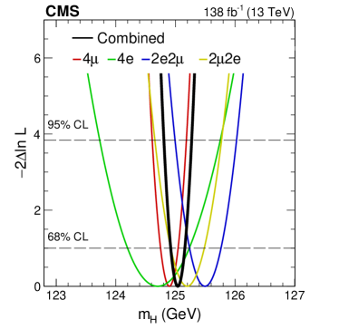
Figure 8: The profile likelihood from the $m_{\PH}$ fit using the $\mathcal{N}$–2D${}^{\prime}_{\text{BS}}$ model for each of the 4$\Pell$ categories and combined. The change in likelihood corresponding to 68 and 95% CLs are shown by the dashed horizontal lines. Both statistical and systematic uncertainties are included in the fits.

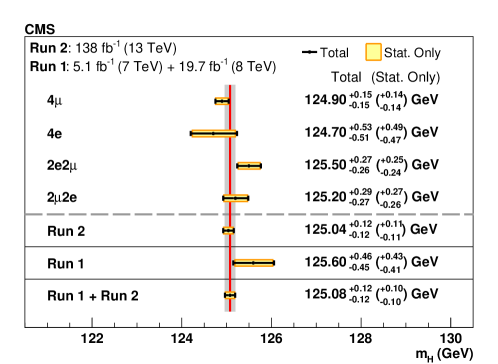
Figure 9: Summary of the CMS Higgs boson mass measurements using the four-lepton final state. The red vertical line and the gray column represent the best fit value and the total uncertainty, respectively, as measured by combining the Runs 1 and 2 data. The yellow band and horizontal black bars show the statistical and total uncertainties in each measurement, respectively. The value of each measurement is given, along with the total and statistical only (in parentheses) uncertainties.

0.10.2 Higgs boson width measurement from on-shell production

The Higgs boson width is measured using on-shell production by fitting the $m_{4\Pell}$ distribution in the mass range $105<m_{4\Pell}<140\GeV$. The $\mathcal{N}$–2D${}^{\prime}_{BS}$ model used for the mass measurement is adopted also in this case, changing the signal model, as described before, to include the $\Gamma_{\PH}$ parameter. Since the theoretical value is very close to zero, which is a strict lower bound, confidence intervals for the Higgs boson width are obtained following the Feldman–Cousins approach [FC]. The is evaluated for several width hypotheses using distributions obtained from simulated pseudo-experiments. In this process, the nuisance parameters are fixed to their best fit values. The observed (expected) upper limit on $\Gamma_{\PH}$ is 50 (320)at 68% and 330 (640)at 95% . Although the observed limit is much less than the expected one, the two are statistically compatible. The resulting distribution of $1-\CL$ vs. $\Gamma_{\PH}$ is shown in Fig. 10.

Figure 10: Distribution of $1-\CL$ vs. $\Gamma_{\PH}$ from the fit in the measurement of the Higgs boson width using on-shell production only. The values shown by the points are extracted using the Feldman-Cousins approach. The vertical bars on the points represent the spread of the simulated pseudo-experiment values. The 68 and 95% values are shown by the dashed horizontal lines.

0.11 Higgs boson width measurement with off-shell production

We perform an extended binned maximum likelihood fit to the on- and off-shell events split in several categories. The final measurements on $m_{\PH}$, $\Gamma_{\PH}$, and $\mu_{j}$ are conducted using the profile likelihood method [cmscollaboration2024cms] implemented in the RooFit toolkit [Verkerke:2003ir] within the root [Brun:1997pa] framework. The extended likelihood function is constructed using the probability densities in Eqs. (5) and (7), with each event characterized by the discrete category $k$ and typically three observables $\vec{x}$. The likelihood $\mathcal{L}$ is maximized with respect to the nuisance parameters $\vec{\xi}_{jk}$ describing the systematic uncertainties and the signal strength parameters $\mu$ (total signal strength), or $\mu_{\cmsSymbolFace{F}}$ (signal strength for $\Pg\Pg\PH$) and $\mu_{\PV}$ (signal strength for the EW processes). The allowed 68 and 95%intervals are defined using the profile likelihood function, $-2\Delta\ln\mathcal{L}=1.00$ and $3.84$, respectively, for which exact coverage is expected in the asymptotic limit [Wilks:1938dza].

Constraints on $\Gamma_{\PH}$ are set by simultaneously fitting $\PH\to\PZ\PZ\to 4\Pell$ events from the on- and off-shell regions. The on-shell region corresponds to Scheme 2 in Ref. [CMS:2021nnc], where six mutually exclusive event categories are defined and anomalous interactions are constrained to zero. It determines the signal strengths $\mu^{\text{on-shell}}_{\cmsSymbolFace{F}}$ and $\mu^{\text{on-shell}}_{\PV}$, corresponding to production mechanisms driven by fermion and vector boson couplings of the Higgs boson, respectively, as defined in Section 0.1. The Higgs boson mass is constrained to $m_{\PH}=125.38$ [Sirunyan:2020xwk] in this fit. In the on- and off-shell parametrizations in Eqs. (5) and (7), we set $\mu^{\text{on-shell}}_{\cmsSymbolFace{F}}=\mu^{\text{off-shell}}_{\cmsSymbolFace{F}}$ and $\mu^{\text{on-shell}}_{\PV}=\mu^{\text{off-shell}}_{\PV}$. The observed and expected constraints on the Higgs boson width are shown in Table 0.11. The likelihood scan of $\Gamma_{\PH}$ using the asymptotic approximation method is shown in Fig. 11. This measurement excludes the scenario of no off-shell Higgs boson production with a corresponding to 3.0 standard deviations (average expected 1.4).

Summary of the total Higgs boson width $\Gamma_{\PH}$ measurement, showing the 68% (central values with uncertainties) and 95% (in square brackets) intervals for the $\PH\to\PZ\PZ\to 4\Pell$ channel alone and in combination with the off-shell $\PH\to\PZ\PZ\to 2\Pell 2\PGn$ channel. lll Channel Observed $\Gamma_{\PH}$ () Expected $\Gamma_{\PH}$ ()
$4\Pell$ on- and off-shell $2.9^{+2.3}_{-1.7}\ [0.3,7.9]$ $4.1\pm 4.0\ [<11.5]$
$4\Pell$ on- and off-shell + $2\Pell 2\PGn$ off-shell $3.0^{+2.0}_{-1.5}\ [0.6,7.3]$ $4.1\pm 3.5\ [0.1,10.5]$

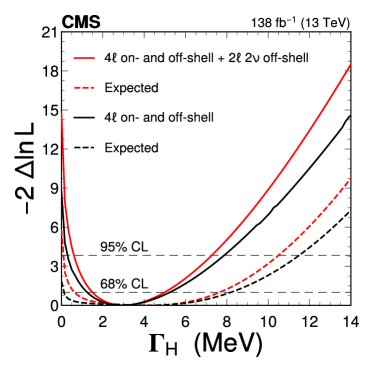
Figure 11: Observed (solid) and expected (dashed) profile likelihood projections from the Higgs boson width fit using on- and off-shell production from this analysis. The analysis of the off-shell $\PH\to\PZ\PZ\to 4\Pell$ channel combined with the on-shell $\PH\to\PZ\PZ\to 4\Pell$ channel [CMS:2021nnc] is shown in black. The full combination of $\PH\to\PZ\PZ\to 4\Pell$ with the off-shell $\PH\to\PZ\PZ\to 2\Pell 2\PGn$ [CMS:2022ley] is given in red. The black horizontal dashed lines show the 68 and 95% values.

The observed limits on $\Gamma_{\PH}$ are stronger than the average expected values from simulation. This is supported by the upper left plot of Fig. 5, where the number of observed events in the sensitive region of $m_{4\Pell}>340$and ${\mathcal{D}}_{\text{bkg}}>0.6$ in the Untagged category is below the expected value, but still consistent with it. The smaller number of events in this region favors the hypothesis of negative interference between the signal and background contributions, which dominates over the pure signal contributions for $\Gamma_{\PH}$ values near the SM value. Therefore, large and very small values of $\Gamma_{\PH}$ are disfavored.

0.11.1 Examination of model dependency in width measurement

The above $\Gamma_{\PH}$ constraints assume the expected SM-like evolution of the Higgs boson couplings over a large $m_{4\Pell}$ range. The anomalous contributions to the $\PH{\PV\PV}$ vertex in EW production and Higgs boson decay were evaluated in our earlier analyses using a smaller data set [Sirunyan:2019twz, CMS:2022ley], and the constraints on $\Gamma_{\PH}$ remained consistent. However, the predominance of the top quark in the $\Pg\Pg\PH$ loop is assumed here and in our previous analyses. If there are additional contributions, such as from yet undiscovered heavy particles, then the $m_{4\Pell}$ evolution in the off-shell region would be altered.

To investigate the impact of large-mass yet undiscovered particles in the $\Pg\Pg\PH$ loop, we introduce a new heavy quark $\PQQ$ with an unconstrained coupling strength $\kappa_{\PQQ}$ in the likelihood parametrization, as described in Refs. [Gritsan:2020pib, Davis:2021tiv]. In the framework of effective field theories, the contribution of $\PQQ$ can be interpreted as a point-like interaction that encapsulates the influence of any heavy particles present in the loop. The parameterization in Eq. (7) is extended to include the templates for terms proportional to $\kappa^{2}_{\PQQ}$ and $\kappa_{\PQQ}$, utilizing simulations reweighted with the mela package in the limit of the infinite $\PQQ$ mass. The $m_{4\Pell}$ shape in the off-shell region shows contrasting patterns between the SM $\Pg\Pg\PH$ production, which is mainly affected by the top quark loop with the $2m_{\PQt}$ threshold effect, and the Higgs boson produced via $\Pg\Pg\PH$ loop involving the heavy quark $\PQQ$ [Gritsan:2020pib].

An unconstrained $\kappa_{\PQQ}$ introduces additional uncertainty into the $m_{4\Pell}$ dependence in the off-shell region, resulting in less stringent limits on $\Gamma_{\PH}$. However, both on- and off-shell $\PH\to 4\Pell$ data constrain the possible values of $\kappa_{\PQQ}$, and the constraints on $\Gamma_{\PH}$ remain largely consistent with those for $\kappa_{\PQQ}=0$. The resulting $\Gamma_{\PH}$ measurement from the combined on- and off-shell events is $2.7^{+2.7}_{-1.8}\MeV$ (expected $4.1^{+5.3}_{-4.0}\MeV$). The observed (expected) 95%  interval is $\,[0.1,8.7]\,(\,[{<}14.1]\,)$. We note that combining measurements from other on-shell Higgs boson production and decay channels in the future will lead to much stricter constraints on $\kappa_{\PQQ}$, reducing the flexibility to alter the SM-like evolution of the Higgs boson couplings over a large $m_{4\Pell}$ range.

0.11.2 Higgs boson width measurement with a combination of off-shell channels

The results of this analysis with the SM-like couplings are combined with the prior CMS off-shell $\PH\to\PZ\PZ\to 2\Pell 2\PGn$ analysis [CMS:2022ley], giving the first CMS measurement of $\Gamma_{\PH}$ using the full $4\Pell$ and $2\Pell 2\PGn$ data sample collected during Run 2. The observed and expected $\Gamma_{\PH}$ measurements are shown in Table 0.11 and Fig. 11 and supersede the previous CMS results [CMS:2022ley] under the SM-like coupling assumption. The fit results rule out the scenario of no off-shell Higgs boson production with a corresponding to 3.8 standard deviations (average expected 2.4).

The off-shell region fit can also be performed without relating its signal strength to that for the on-shell region. In this case, the signal strength is modified by the parameter $\mu^{\text{off-shell}}$ common to all production mechanisms, with $\Gamma_{\PH}=\Gamma_{\PH}^{\mathrm{SM}}$ in Eq. (7), and the SM expectation corresponding to $\mu^{\text{off-shell}}=1$. In addition, we also perform a fit of the off-shell events with two unconstrained parameters $\mu^{\text{off-shell}}_{\cmsSymbolFace{F}}$ and $\mu^{\text{off-shell}}_{\PV}$, which express the signal strengths in the $\Pg\Pg\PH$ and EW processes, respectively. The measured signal strengths are reported in Table 0.11.2 and a 2D scan of these parameters is presented in Fig. 12. The observed limits on signal strength in the off-shell region are stronger than expected on average, following a trend similar to that previously discussed for $\Gamma_{\PH}$.

Measured values of the signal strengths $\mu^{\text{off-shell}}$, $\mu_{\cmsSymbolFace{F}}^{\text{off-shell}}$, and $\mu_{\PV}^{\text{off-shell}}$, and their 68% and 95% (in square brackets) intervals from the combined fit to the off-shell $\PH\to\PZ\PZ\to 4\Pell$ and $2\Pell 2\PGn$ channels. lcc Parameter Observed Expected
$\mu^{\text{off-shell}}$ $0.67^{+0.42}_{-0.32}\ [0.14,1.54]$ $1.00^{+0.83}_{-0.84}\ [0.02,2.46]$
$\mu_{\cmsSymbolFace{F}}^{\text{off-shell}}$ $0.57^{+0.50}_{-0.36}\ [0.04,1.61]$ $1.00^{+0.90}_{-0.98}\ [{<}2.62]$
$\mu_{\PV}^{\text{off-shell}}$ $0.87^{+0.93}_{-0.57}\ [0.05,2.90]$ $1.00^{+1.95}_{-0.89}\ [{<}4.34]$

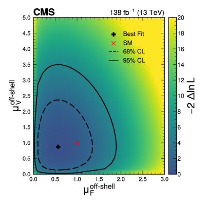
Figure 12: Observed 2D profile likelihood projection of the off-shell signal strength parameters ($\mu^{\text{off-shell}}_{\cmsSymbolFace{F}}$, $\mu^{\text{off-shell}}_{\PV}$) from the fit to the combined off-shell $\PH\to\PZ\PZ\to 4\Pell$ and $2\Pell 2\PGn$ channels. The best fit value is shown by the black cross and the SM prediction by the red x. The 68 and 95% contours are given by the dashed and solid curves, respectively. The color scale to the right of the plot relates the quantitative values.

0.12 Summary

A measurement of the Higgs boson mass ($m_{\PH}$) and width ($\Gamma_{\PH}$) using the decays to two bosons is presented. The data sample comes from proton-proton collisions at the LHC recorded by the CMS experiment at a center-of-mass energy of 13, corresponding to an integrated luminosity of 138. On-shell Higgs boson production with the $\PH\to 4\Pell$ decay ($\Pell=\Pe$, $\PGm$) is used to measure its mass and constrain its width. The mass measurement yields $m_{\PH}=125.04\pm 0.11\stat\pm 0.05\syst\GeV=125.04\pm 0.12$, in agreement with the expected precision of $\pm$0.12. From on-shell production events, an upper limit of $\Gamma_{\PH}<330\MeV$ is set at 95% confidence level. The mass measurement is further improved combining data from Runs 1 and 2, leading to the most precise single measurement of the mass to date in this channel, $m_{\PH}=125.08\pm 0.10\stat\pm 0.05\syst\GeV=125.08\pm 0.12$. Using on- and off-shell Higgs boson production with the decay to four leptons, and combining them with a separate analysis with Higgs boson decay to two leptons plus two neutrinos, we measure $\Gamma_{\PH}=3.0^{+2.0}_{-1.5}\MeV$, consistent with the standard model prediction of 4.1. These results are summarized in Table 0.12. The strength of the off-shell Higgs boson production is also reported, and the scenario of no off-shell Higgs boson production is excluded at a confidence level corresponding to 3.8 standard deviations. Results of the measurements are tabulated in the HEPData record for this analysis [hepdata].

Summary of the Higgs boson mass and total width $\Gamma_{\PH}$ measurements, showing the allowed 68% (central values with uncertainties) and 95% (in square brackets) intervals. Uncertainties are reported as a combination of statistical and systematic uncertainties. The first two rows display the outcomes of the analysis conducted within the on-shell $\PH\to\PZ\PZ\to 4\Pell$ region, where the width is restricted to be positive. The third row incorporates results from the off-shell $\PH\to\PZ\PZ\to 4\Pell$ region combined with the on-shell $\PH\to\PZ\PZ\to 4\Pell$ [CMS:2021nnc] and off-shell $\PH\to\PZ\PZ\to 2\Pell 2\PGn$ [CMS:2022ley]. lcc Parameter Observed Expected
$m_{\PH}$ () $125.08\pm 0.12$ $\pm 0.12$
on-shell $\Gamma_{\PH}$ () $<$50 $[{<}330]$ $<$320 $[{<}640]$
off-shell $\Gamma_{\PH}$ () $3.0^{+2.0}_{-1.5}\ [0.6,7.3]$ $4.1\pm 3.5\ [0.1,10.5]$