Hölder curves with exotic tangent spaces

Abstract.

An important implication of Rademacher’s Differentiation Theorem is that every Lipschitz curve $\Gamma$ infinitesimally looks like a line at almost all of its points in the sense that at $\mathcal{H}^{1}$-almost every point of $\Gamma$, the only weak tangent to $\Gamma$ is a straight line through the origin. In this article, we show that, in contrast, the infinitesimal structure of Hölder curves can be much more extreme. First we show that for every $s>1$ there exists a $(1/s)$-Hölder curve $\Gamma_{s}$ in a Euclidean space with $\mathcal{H}^{s}(\Gamma_{s})>0$ such that $\mathcal{H}^{s}$-almost every point of $\Gamma_{s}$ admits infinitely many topologically distinct weak tangents. Second, we study the weak tangents of self-similar connected sets (which are canonical examples of Hölder curves) and prove that infinitely many of the curves $\Gamma_{s}$ have the additional property that $\mathcal{H}^{s}$-almost every point of $\Gamma_{s}$ admits a weak tangent to $\Gamma_{s}$ which is not admitted as (not even bi-Lipschitz to) a weak tangent to any planar self-similar set at typical points.

1. Introduction

Rademacher’s Theorem, one of the most important theorems in geometric measure theory, states that every Lipschitz function defined on $[0,1]$ is differentiable at $\mathcal{H}^{1}$-almost every point of $[0,1]$. It is natural to ask whether a similar result may hold for more general functions. Calderon [Cal51] extended Rademacher’s Theorem by proving that every function in the Sobolev class $\mathcal{W}^{1,p}$ with $p>1$ is $\mathcal{H}^{1}$-almost everywhere differentiable. However, any further generalization would be futile as for each $s>1$ there exists a Weierstrass function on $[0,1]$ which is $\frac{1}{s}$-Hölder but nowhere differentiable [Zyg02].

A major application of Rademacher’s Theorem is towards the understanding of the “infinitesimal structure” of Lipschitz curves (i.e. Lipschitz images of $[0,1]$). To state this application, let us first define the notion of weak tangents. Given a closed set $X\subset\mathbb{R}^{n}$ and a point $x\in X$, we say that a closed set $T$ is a weak tangent of $X$ at $x$ if there exists a sequence of positive scales $r_{j}$ that go to zero such that the blow-up sets $r_{j}^{-1}(X-x)$ converge to the set $T$ in the Attouch-Wets topology; see §2.4 for the precise definition. Other notions of metric space convergences which produce similar weak tangents are known in the literature; see [Gro81, Gro99, DS97]. Another well-known notion of infinitesimal structure in geometric measure theory is that of the tangent cone [Fed69, 3.1.21]. The tangent cone of $X$ at $x$ is the union of all weak tangents of $X$ at $x$, which means that some local information is lost. We denote by $\operatorname{Tan}(X,x)$ the collection of all weak tangent of $X$ at $x$. It is well-known that $\operatorname{Tan}(X,x)$ is nonempty and that if $T$ is in $\operatorname{Tan}(X,x)$, then $\lambda T$ is in $\operatorname{Tan}(X,x)$ for every $\lambda>0$.

By Rademacher’s Theorem and by a theorem of Besicovitch [Bes44] (see also [Fal86, Corollary 3.15]), every Lipschitz curve is infinitesimally a line at $\mathcal{H}^{1}$-almost every point. More precisely, the following is true, and we provide a proof in Section 3.

Proposition 1.1.

If $f:[0,1]\to\mathbb{R}^{N}$ is Lipschitz, then for $\mathcal{H}^{1}$-a.e. $x\in f([0,1])$, there exists a straight line $L\subset\mathbb{R}^{N}$ through the origin such that $\operatorname{Tan}(f([0,1]),x)=\{L\}$.

More generally, if $X$ is the Lipschitz (or even $p$-Sobolev for $p>n$) image of $[0,1]^{n}$ into some $\mathbb{R}^{m}$ with $m>n$, then for $\mathcal{H}^{n}$-a.e. $x\in X$, the tangent space of $X$ at $x$ (in the pointed Gromov-Hausdorff sense) contains exactly one element which is an $n$-plane [BKV24]. Here and for the rest of this paper, given $\alpha>0$, we denote by $\mathcal{H}^{\alpha}(X)$ the Hausdorff $\alpha$-dimensional measure of a metric space $X$.

It is worthwhile to note that while typical points of a Lipschitz curve have a simple tangent space, exceptional points may exhibit extreme behaviors. In particular, there exists a Lipschitz curve $\Gamma\subset\mathbb{R}^{2}$ (or in any Euclidean space of dimension at least $2$) and a point $x_{0}\in\Gamma$ such that $\operatorname{Tan}(\Gamma,x_{0})$ contains every possible weak tangent; see Appendix A for a precise statement and the proof.

The infinitesimal structure of Lipschitz curves plays an important role in the classification of 1-rectifiable sets by Jones [Jon90] and Okikiolu [Oki92]. A feature of the proofs is the use of Jones’s beta numbers, which roughly measure how well a given set $E$ can be approximated by lines at a given scale and location, and showing that if these values are small enough at all scales and locations then $E$ can be captured in a rectifiable curve. Roughly speaking, a set $E$ is contained in a Lipschitz curve if and only if at almost all points, tangent spaces are lines in a strong quantitative way. For a more complete discussion of the history of the Analyst’s Traveling Salesperson Theorem, see [Sch07] and the citations therein.

Recent years have seen great interest in obtaining a Hölder version of the Analyst’s Traveling Salesperson Theorem, that is, in characterizing all sets which are contained in a Hölder curve; see for example [MM93, Rem98, MM00, BV17, BNV19, BZ20, BV21, SV24, BS23]. This notion of “Hölder rectifiability” is greatly motivated by the fact that many fractals in analysis on metric spaces admit a Hölder parameterization but not a Lipschitz one. For example, if the attractor of an iterated function system is connected (e.g. the von Koch curve, the Sierpiński gasket, the Sierpiński carpet), then it admits a Hölder parameterization by $[0,1]$; see [Rem98, BV21].

In lieu of the Lipschitz rectifiability results discussed above, a crucial step towards a comprehensive theory of Hölder rectifiable sets would be to understand the tangent spaces of Hölder curves at typical points. Unfortunately, unlike the Lipschitz case, it would be naive to expect that given $s>1$ there exists one single set $T_{s}$ which is the weak tangent of all $\frac{1}{s}$-Hölder curves at typical points. For example, consider the two self similar sets $\mathcal{S}$ and $\mathcal{C}$ constructed as follows. Set $S_{0}=T$ where $T$ is be an isosceles triangle with side-lengths $1,5^{-1/4},5^{-1/4}$, and for each $n\in\mathbb{N}$ set $S_{n}=\phi_{1}(S_{n-1})\cup\phi_{2}(S_{n-1})$ where $\phi_{1},\phi_{2}$ are the two similarities in the left image of Figure 1. The sets $S_{n}$ converge to a snowflake-like curve $\mathcal{S}=\bigcap_{n\in\mathbb{N}}S_{n}$. Similarly, set $C_{0}=[0,1]^{2}$ and for each $n\in\mathbb{N}$ set $C_{n}=\bigcup_{i=1}^{16}\psi_{i}(C_{n-1})$ where $\psi_{1},\dots,\psi_{16}$ are the similarities in the right image of Figure 1. The sets $C_{n}$ converge to a carpet-like set $\mathcal{C}=\bigcap_{n\in\mathbb{N}}S_{n}$. Both $\mathcal{S}$ and $\mathcal{C}$ are connected self-similar sets which have Hausdorff dimension equal to $s=\log{16}/\log{5}$ and positive $\mathcal{H}^{s}$ measure, and by a theorem of Remes [Rem98], both are $\frac{1}{s}$-Hölder curves. However, the tangents of $\mathcal{S}$ at $\mathcal{H}^{s}$-a.e. point are infinite snowflakes while the tangents of $\mathcal{C}$ at $\mathcal{H}^{s}$-a.e. point are infinite carpets; hence they are topologically different.

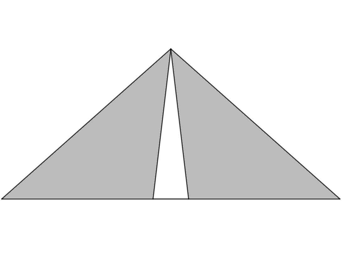
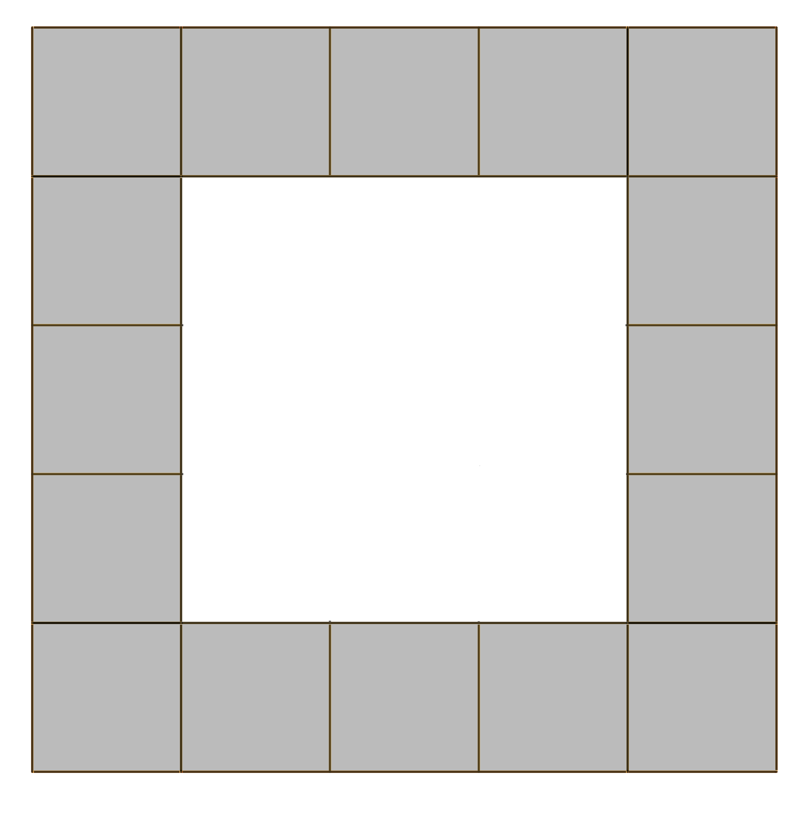
Figure 1. First stages of sets $\mathcal{S}$ (left) and $\mathcal{C}$ (right).

The previous two examples lead us to ask whether there are infinitely many Hölder curves $\Gamma_{1},\Gamma_{2},\dots$ and infinitely many sets $T_{1},T_{2},\dots$ such that $T_{i}$ are pairwise topologically different and each $T_{i}$ is a weak tangent of $\Gamma_{i}$ at typical points. In our main result, we show that not only is this true but it is even worse: this situation can arise in one single Hölder curve. Furthermore, the Hölder exponent of such a curve can be chosen arbitrarily close to 1.

Theorem 1.2.

For each $s>1$, there exists a $\frac{1}{s}$-Hölder curve $\Gamma_{s}$ in some Euclidean space such that $\mathcal{H}^{s}(\Gamma_{s})>0$ and for $\mathcal{H}^{s}$-almost every $x\in\Gamma_{s}$, the space $\operatorname{Tan}(\Gamma_{s},x)$ contains infinitely many topologically different weak tangents.

We note that little is currently known about the geometry of weak tangents at typical points. For example, are weak tangents at typical points connected? If so, are they Hölder images of $\mathbb{R}$? Proposition 1.1 answers the previous two questions in the affirmative for Lipschitz curves.

1.1. Weak tangents of self-similar sets

Recall that an iterated function system (abbv. IFS) of similarities on $\mathbb{R}^{n}$ is a finite collection $\mathcal{F}$ of contracting similarities of $\mathbb{R}^{n}$. We say that a set $K$ is the attractor of an IFS $\mathcal{F}$ if $K=\bigcup_{\phi\in\mathcal{F}}\phi(K)$. An IFS $\mathcal{F}$ satisfies the open set condition (abbv. OSC) if there exists an open set $U\subset\mathbb{R}^{n}$ such that for all distinct $\phi,\phi^{\prime}\in\mathcal{F}$ we have $\phi(U)\subset U$ and $\phi(U)\cap\phi^{\prime}(U)=\emptyset$. In this paper, we say that a set $Q$ is self-similar if it is the attractor of an IFS of similarities with the OSC. A well-known theorem of Hutchinson [Hut81] states that every self-similar set has finite and positive $\mathcal{H}^{s}$-measure for some $s>0$.

Perhaps the richest source of Hölder curves with positive and finite Hausdorff measure is that of self-similar sets. While there are examples of Hölder curves with positive and finite Hausdorff measure which are not self-similar sets (e.g. a bi-Lipschitz embedding of the snowflaked space $([0,1],|\cdot|^{\epsilon})$ [BH04, Wu15, RV17]), these examples are all bi-Lipschitz equivalent to self-similar sets. Therefore, it is natural to ask if Hölder curves have weak tangents possessing some form of self-similarity at typical points. Note that weak tangents of Lipschitz curves at typical points are straight lines which do possess local self-similarity. This discussion motivates two questions. First, can we classify weak tangents of (connected) self-similar sets? Second, are weak tangents of general Hölder curves always bi-Lipschitz equivalent to weak tangents of connected self-similar sets?

In pursuit of the first of question, we investigate the weak tangents of self-similar sets and we show that if $Q$ is a self-similar set in Euclidean space, then at $\mathcal{H}^{\operatorname{dim_{H}}(Q)}$-almost every point $x$ of $Q$, every weak tangent is locally made up of “big pieces of $Q$”.

Proposition 1.3.

Let $\{\phi_{i}:\mathbb{R}^{N}\to\mathbb{R}^{N}\}_{i=1}^{m}$ be an IFS of similarities satisfying the OSC for some open set $U$, let $Q$ be the attractor, and let $s=\operatorname{dim_{H}}{Q}$. Assume $U\cap Q\neq\emptyset$. There exists $c_{0}\in\mathbb{N}$ depending only on the Lipschitz norms of $\phi_{1},\dots,\phi_{m}$ such that for $\mathcal{H}^{s}$-almost every $x\in Q$, every weak tangent $T\in\operatorname{Tan}(Q,x)$, and every $R>0$, there exist similarities $\{f_{i}^{R}:Q\to T\}_{i=1}^{M_{R}}$ with $M_{R}\leq c_{0}$ with Lipschitz norms in $[c_{0}^{-1}R,R]$ such that

$$\overline{B}({\bf 0},R)\cap T\subset\bigcup\limits_{j=1}^{M_{R}}f_{j}^{R}(Q)\subset\overline{B}({\bf 0},2R)\cap T$$

and for all distinct $i,j\in\{1,\dots,M_{R}\}$, $f_{i}^{R}(U)\cap f_{j}^{R}(U)=\emptyset$, $f_{i}^{R}(U\cap Q)$ is an open subset of $T$.

Here we denote by ${\bf 0}$ the origin in $\mathbb{R}^{N}$. For the special case of self-similar sponges (which includes self-similar carpets such as the Sierpiński carpet), we show in Section 10 that at typical points of the sponge, each weak tangent is locally self-similar, which means roughly that every open ball contains a similar copy of every other open ball as an open subset.

Regarding the second question, following the construction in Theorem 1.2, we show in Section 10 that there exist Hölder curves which infinitesimally, do not resemble self-similar sets.

Theorem 1.4.

For each $\epsilon>0$ there exists $s\in(1,1+\epsilon)$ and a $\frac{1}{s}$-Hölder curve $\Gamma_{s}\subset\mathbb{R}^{2}$ such that $\mathcal{H}^{s}(\Gamma_{s})>0$, and such that at $\mathcal{H}^{s}$-a.e. point $x\in\Gamma_{s}$ there exists $T\in\operatorname{Tan}(\Gamma_{s},x)$ with the following property. If $Q\subset\mathbb{R}^{2}$ is a self-similar set with $\operatorname{dim_{H}}{Q}=s$, then the set of points $z\in Q$ for which $T$ is bi-Lipschitz homeomorphic to an element of $\operatorname{Tan}(Q,z)$ is $\mathcal{H}^{s}$-null.

To the best of our knowledge, the curves of Theorem 1.4 are the first examples of Hölder curves that $\mathcal{H}^{s}$-almost everywhere possess weak tangents which are not realizable as a weak tangent of a self-similar set at $\mathcal{H}^{s}$-almost any point. However, it is worthwhile noting that the Hölder curves of Theorem 1.4 have the property that at typical points, some weak tangent does arise as a weak tangent of a self-similar set at typical points. In light of this, we leave open a weakened version of the second question as a conjecture, originally due to Matthew Badger and the second named author in 2019.

Question 1.5 (Badger, Vellis).

If $\Gamma$ is a Hölder curve in Euclidean space, then is it true that at typical points, there is some weak tangent which is bi-Lipschitz to a weak tangent of a connected self-similar set at typical points?

1.2. Outline of the proof of Theorem 1.2

To simplify the exposition, we first describe the construction of $\Gamma_{s}$ in the special case that $s=\log{24}/\log{6}$. The set $\Gamma_{s}$ is constructed by applying two sets of iterated function systems on $\mathbb{R}^{2}$ in a somewhat random fashion. We start with the unit square $\mathcal{S}^{0}$. Assume now that for some $k\geq 0$ we have defined $\mathcal{S}^{k}$ which is the union of $24^{k}$ closed squares $\mathcal{S}^{k}_{w}$ with disjoint interiors. Each such square is replaced by a copy of Model 1 or a copy of Model 2 in Figure 2, rescaled by $6^{-k}$. After replacing each square, we obtain $\mathcal{S}^{k+1}$. We have that $\mathcal{S}^{0}\supset\mathcal{S}^{1}\supset\cdots$ and the set $\Gamma_{s}$ is the Hausdorff limit of these sets. The choice between Model 1 or Model 2 at every stage of the construction is encoded by a choice function $\eta$ which is defined on all finite words made from characters $\{1,\dots,24\}$ and takes values in $\{1,2\}$. See Section 4 for the rigorous construction. The important detail is that Model 1 contains one local cut-point (i.e. a point $x$ which if removed makes a neighborhood of $x$ disconnected) while Model 2 has no such point.

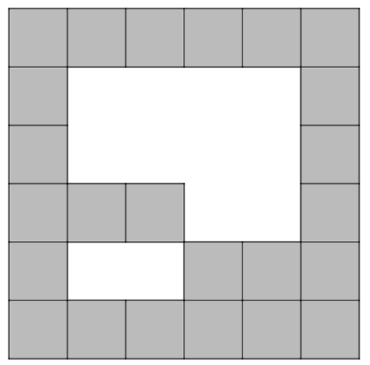
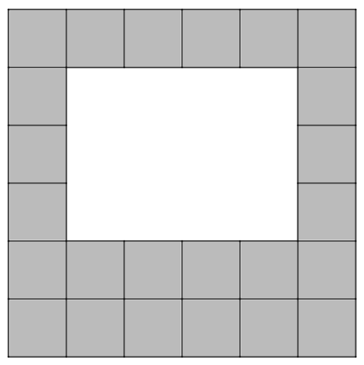
Figure 2. Model 1 (left) and Model 2 (right) for $s=\log{24}/\log{6}$.

In Section 5 we show that, no matter what the choice function $\eta$ is, the resulting “limit set” $\Gamma_{s}$ will satisfy $0<\mathcal{H}^{s}(\Gamma_{s})<\infty$. Then, in Section 6, drawing inspiration from the techniques in parametrization results of attractors of iterated function systems (e.g. in [Hat85] and [BV21]), for each choice function $\eta$, we construct Lipschitz curves which approximate $\Gamma_{s}$ and converge to a $\frac{1}{s}$-Hölder parameterization of $\Gamma_{s}$.

Note that if a choice function takes only one value (say 1), then the resulting set $\Gamma_{s}$ is self-similar, and in fact, a self-similar sponge which, as we prove, have very nice tangent spaces; see §10.1. Thus in order to obtain a set where at typical points, the tangent space contains infinitely many topologically different elements which cannot be obtained from a self-similar set, the choice function necessarily must exhibit some form of randomness. In Section 7, using a measure-theoretic argument on the set of choice functions, we show that almost every choice function (in terms of a suitable probability measure) yields a continuum $\Gamma_{s}$ which “sees” both models in arbitrarily small neighborhoods at $\mathcal{H}^{s}$-almost every point. With such a choice function in hand, we show in Section 8 that at $\mathcal{H}^{s}$-almost every $x\in\Gamma_{s}$, and for each $k\in\mathbb{N}$, there exists a weak tangent $T\in\operatorname{Tan}(\Gamma_{s},x)$ that contains exactly $\frac{1}{23}(24^{k}-1)$ many local cut-points (see §2.5). Therefore, there are infinitely many topologically different weak tangents.

A construction similar to the one described above works for all values $s$ of the form $\alpha_{n}=\frac{\log(5n-6)}{\log(n)}$ where $n\geq 4$ is an even number. To obtain Theorem 1.2 for an arbitrary $s>1$, we first choose $n\geq 4$ even such that $s>\alpha_{n}$. Then in Section 9 we appropriately “snowflake” the curve $\Gamma_{\alpha_{n}}$, apply Assouad’s embedding theorem [Ass83] to bi-Lipschitz embed the snowflaked $\Gamma_{\alpha_{n}}$ into some Euclidean space, and use a weak-tangent-snowflaking argument to show that the embedded image (which has dimension $s$) satisfies the conclusions of Theorem 1.2.

Finally, in Section 10 we prove that these weak tangents cannot be obtained as weak tangents of planar self-similar sets at generic points.

2. Preliminaries

2.1. Dendrites

A dendrite is a Peano continuum (that is, compact, connected, and locally connected at every point) which contains no simple closed curves. The leaves of a dendrite $X$ are exactly those points $x\in X$ such that $X\setminus\{x\}$ is connected.

Lemma 2.1.

Let $T_{1},T_{2}$ be two dendrites in $\mathbb{R}^{n}$ that intersect on a point. Then $T_{1}\cup T_{2}$ is a dendrite.

Proof.

Recall that a metric space is a dendrite if and only if any two distinct points can be separated by a third point [Nad92, Theorem X.10.2]. Suppose that $T_{1}\cap T_{2}=\{x_{0}\}$. Fix distinct $x,y\in T_{1}\cup T_{2}$. If $x,y\in T_{1}$, since $T_{1}$ is a dendrite, there exists a point $z\in T_{1}$ that separates $x$ and $y$. Similarly if $x,y\in T_{2}$. If $x\in T_{1}\setminus T_{2}$ and $y\in T_{2}\setminus T_{1}$, then $x_{0}$ separates $x$ and $y$. ∎

2.2. Words

For each even positive integer $n\geq 4$ we denote

$$\mathcal{A}_{n}=\{1,\dots,5n-6\}.$$

Given $n$ as above and integer $m\geq 0$, let $\mathcal{A}_{n}^{m}$ be the set of words of length $m$ formed by characters in $\mathcal{A}_{n}$, with the convention that $\mathcal{A}_{n}^{0}=\{\varepsilon\}$, where $\varepsilon$ is the empty word. Define $\mathcal{A}_{n}^{*}:=\bigcup_{m=0}^{\infty}\mathcal{A}_{m}^{m}$ and $\mathcal{A}_{n}^{\mathbb{N}}$ be the set of infinitely countable words.

Given a word $w\in\mathcal{A}_{n}^{*}$, we denote by $|w|$ the length of $w$. Also, given $w=i_{1}\cdots i_{m}\in\mathcal{A}_{n}^{m}$ and $j\leq m$, we write $w(j)=i_{1}\cdots i_{j}$. For any $w\in\mathcal{A}_{n}^{*}$, define the cylinder set $\mathcal{A}_{n,w}^{\mathbb{N}}:=\{\tau\in\mathcal{A}_{n}^{\mathbb{N}}:\tau(m)=w\}$, that is, the set of infinite words which agree with $w$ for the first $m$ characters. Similarly, for $j,m\in\mathbb{N}$ with $m\geq j$ and for each $w\in\mathcal{A}_{n}^{j}$, we define $\mathcal{A}_{n,w}^{m}:=\{v\in\mathcal{A}_{n}^{m}:v(j)=w\}$.

Denote by $\Sigma_{n}$ the $\sigma$-algebra generated by the cylinders $\mathcal{A}^{\mathbb{N}}_{n,w}$ where $w\in\mathcal{A}_{n}^{*}$. Then there exists a unique probability measure $\nu_{n}:\Sigma_{n}\to[0,1]$ such that $\nu_{n}(\mathcal{A}^{\mathbb{N}}_{n,w})=(5n-6)^{-|w|}$ for all $w\in\mathcal{A}_{n}^{*}$; see for example [Str93, §3.1].

2.3. Combinatorial graphs and trees

A combinatorial graph is a pair $G=(V,E)$ of a finite or countable vertex set $V$ and an edge set

$$E\subset\{\{v,v^{\prime}\}:v,v^{\prime}\in V\text{ and }v\neq v^{\prime}\}.$$

If $\{v,v^{\prime}\}\in E$, we say that the vertices $v$ and $v^{\prime}$ are adjacent in $G$.

If $V\subset\mathbb{R}^{n}$ for some $n\in\mathbb{N}$, then we define the image of $G$ to be the set

$$\text{Im}(G):=\bigcup_{\{v,v^{\prime}\}\in E}[v,v^{\prime}]$$

where $[v,v^{\prime}]$ denotes the line segment from $v$ to $v^{\prime}$. Recall that if $v\in V$ is a vertex, then the valence of $v$ in $G$ is the number of components of $\text{Im}(G)\setminus\{v\}$.

A simple path in $G$ is a set $\gamma=\{\{v_{1},v_{2}\},\dots,\{v_{n-1},v_{n}\}\}\subset E$ such that for all distinct $i,j\in\{1,\dots,n\}$ we have $v_{i}\neq v_{j}$; in this case we say that $\gamma$ joins $v_{1}$, $v_{n}$. A graph $T=(V,E)$ is a combinatorial tree if for any distinct $v,v^{\prime}$ there exists a unique simple path $\gamma$ that joins $v$ with $v^{\prime}$.

2.4. Weak tangents

If $A$ and $B$ are nonempty subsets of a Euclidean space $\mathbb{R}^{N}$, then we define the excess of A over B as

$$\operatorname{excess}(A,B)=\sup_{a\in A}\inf_{b\in B}|a-b|.$$

See [Bee93, §3.1], [BL15], and [BET17, Appendix A]. In the next remark, we catalogue six important properties of the excess which will be used heavily throughout this article. The first and fifth properties follow straightforwardly from the definition of excess while the other four are given in [BL15, Section 2].

Remark 2.2.

The excess satisfies the following four properties.

1. Translation invariance. For nonempty sets $A,B\subset\mathbb{R}^{N}$ and any point $x\in\mathbb{R}^{N}$,

   $$\operatorname{excess}(A,B)=\operatorname{excess}(A+x,B+x).$$

2. Triangle inequality. For nonempty sets $A,B,C\subset\mathbb{R}^{N}$,

   $$\operatorname{excess}(A,C)\leq\operatorname{excess}(A,B)+\operatorname{excess}(B,C).$$

3. Containment. For nonempty sets $A,B\subset\mathbb{R}^{N}$, $\operatorname{excess}(A,B)=0$ if, and only if, $A\subset\overline{B}$.

4. Monotonicity. If $A\subset A^{\prime}$, $B^{\prime}\subset B$ are all nonempty subsets of $\mathbb{R}^{N}$, then

   $$\operatorname{excess}(A,B)\leq\operatorname{excess}(A^{\prime},B^{\prime}).$$

5. Subadditivity. If $A,B,C\subset\mathbb{R}^{N}$ are all nonempty, then

   $$\operatorname{excess}(A\cup B,C)\leq\operatorname{excess}(A,C)+\operatorname{excess}(B,C).$$

6. Closure. If $A,B\subset\mathbb{R}^{N}$ are nonempty, then

   $$\operatorname{excess}(A,B)=\operatorname{excess}(\overline{A},\overline{B}).$$

Let $\mathfrak{C}(\mathbb{R}^{N})$ be the set of nonempty closed subsets of $\mathbb{R}^{N}$, and let $\mathfrak{C}(\mathbb{R}^{N};{\bf 0})$ be the collection of nonempty closed subsets of $\mathbb{R}^{N}$ containing the origin ${\bf 0}$. We consider both of these spaces equipped with the Attouch-Wets topology, which is defined in [Bee93, Definition 3.1.2].

Lemma 2.3 ([Bee93, Chapter 3]).

There exists a metrizable topology on $\mathfrak{C}(\mathbb{R}^{N})$ in which a sequence of sets $(X_{i})_{i=1}^{\infty}\subset\mathfrak{C}(\mathbb{R}^{N})$ converges to a set $X\in\mathfrak{C}(\mathbb{R}^{N})$ if and only if for every $r>0$,

$$\lim_{m\to\infty}\operatorname{excess}(X_{m}\cap\overline{B}({\bf 0},r),X)=0\quad\text{and}\quad\lim_{m\to\infty}\operatorname{excess}(X\cap\overline{B}({\bf 0},r),X_{m})=0.$$

Moreover, the subcollection $\mathfrak{C}(\mathbb{R}^{N};{\bf 0})$ is sequentially compact; that is, for any sequence $(X_{i})_{i=1}^{\infty}\subset\mathfrak{C}(\mathbb{R}^{N};{\bf 0})$ there exists a subsequence $(X_{i_{j}})_{j=1}^{\infty}$ and a set $X\in\mathfrak{C}(\mathbb{R}^{N};{\bf 0})$ such that $(X_{i_{j}})_{j=1}^{\infty}$ converges to $X$.

In the following lemma, we record a useful property of Attouch-Wets convergence in $\mathfrak{C}(\mathbb{R}^{N};{\bf 0})$, which roughly says that sequences in $\mathfrak{C}(\mathbb{R}^{N};{\bf 0})$ that converge in the Attouch-Wets topology satisfy a type of Cauchy condition with respect to excess.

Lemma 2.4.

If $(A_{j})_{j\in\mathbb{N}}\subset\mathfrak{C}(\mathbb{R}^{N};{\bf 0})$ is a sequence converging to a set $A\in\mathfrak{C}(\mathbb{R}^{N};{\bf 0})$ with respect to the Attouch-Wets topology, then for every $r>0$ and each $\epsilon>0$, there exists an integer $j_{0}\in\mathbb{N}$ so that for every pair of integers $j_{1},j_{2}\geq j_{0}$, $\operatorname{excess}(A_{j_{1}}\cap\overline{B}({\bf 0},r),A_{j_{2}})<\epsilon$.

Proof.

Let $\epsilon>0$ and let $r>0$. Since $A_{j}\to A$ in the Attouch-Wets topology as $j\to\infty$, there exists an integer $j_{0}\in\mathbb{N}$ so that for every integer $j\geq j_{0}$

$$\operatorname{excess}(A_{j}\cap\overline{B}({\bf 0},r),A)<\min\{\epsilon/2,r\}\text{ and }\operatorname{excess}(A\cap\overline{B}({\bf 0},2r),A_{j})<\min\{\epsilon/2,r\}.$$

Then for every pair of integers $j_{1},j_{2}\geq j_{0}$, by the triangle inequality for excess (see Remark 2.2),

$$\operatorname{excess}(A_{j_{1}}\cap\overline{B}({\bf 0},r),A_{j_{2}})\leq\operatorname{excess}(A_{j_{1}}\cap\overline{B}({\bf 0},r),A\cap\overline{B}({\bf 0},2r))+\operatorname{excess}(A\cap\overline{B}({\bf 0},2r),A_{j_{2}}).$$

Now since $j_{1}\geq j_{0}$, $\operatorname{excess}(A_{j_{1}}\cap\overline{B}({\bf 0},r),A)<\min\{\epsilon/2,r\}$, so for every $x\in A_{j_{1}}\cap\overline{B}({\bf 0},r)$ there exists a point $y\in A$ so that $|x-y|<\min\{\epsilon/2,r\}$. Then it must hold that such a point $y$ is contained in $\overline{B}({\bf 0},2r)\cap A$, and therefore $\operatorname{excess}(A_{j_{1}}\cap\overline{B}({\bf 0},r),A\cap\overline{B}({\bf 0},2r))<\epsilon/2$. Additionally, since $j_{2}\geq j_{0}$, we have also that $\operatorname{excess}(A\cap\overline{B}({\bf 0},2r),A_{j_{2}})<\epsilon/2$, and this completes the proof. ∎

Let $X\in\mathfrak{C}(\mathbb{R}^{N})$ and let $x\in X$. We say that a set $T\in\mathfrak{C}(\mathbb{R}^{N};{\bf 0})$ is a weak tangent set of $X$ at $x$ if there exists a sequence of scales $(r_{m})_{m\in\mathbb{N}}>0$ such that $r_{m}\to 0$ and $\frac{X-x}{r_{m}}\to T$ with respect to the Attouch-Wets topology. We denote by $\operatorname{Tan}(X,x)$ the set of all weak tangent sets to $X$ at $x$.

For the next lemma, denote by $\mathfrak{C}_{U}(\mathbb{R}^{N};{\bf 0})$ the collection of all sets $X\in\mathfrak{C}(\mathbb{R}^{N};{\bf 0})$ such that every component of $X$ is unbounded.

Lemma 2.5.

If $X\subset\mathbb{R}^{N}$ is a nondegenerate continuum, then $\operatorname{Tan}(X,x)\subset\mathfrak{C}_{U}(\mathbb{R}^{N};{\bf 0})$ for every $x\in X$.

Proof.

Fix $T\in\operatorname{Tan}(X,x)$ and assume for a contradiction that $T$ has a bounded component $K$.

Let $L$ be the component of $T^{\prime}=T\cup\{\infty\}$ in $\mathbb{S}^{N}$ that contains $\infty$. Then clearly $K,L$ are distinct connected components of $T^{\prime}$. Regarding $K$ and $L$ as quasi-components of $T^{\prime}$, one can choose two disjoint closed sets $Y,Z\subset T^{\prime}$ satisfying $K\subset Y$, $L\subset Z$, and $T^{\prime}=Y\cup Z$. Then both $Y$ and $Z$ are closed in $\mathbb{S}^{N}$, and thus by normality there exists an open set $U$ such that

$$Y\subset U\subset\overline{U}\subset\mathbb{S}^{N}\setminus Z.$$

Since $\infty\notin\overline{U}$, we have that $\overline{U}$ is a compact subset of $\mathbb{R}^{N}$. Set $d=\operatorname{dist}(Z,Y)$.

Fix $R>0$ large enough that $Y\subset\overline{B}({\bf 0},R)$ and $Z\cap\overline{B}({\bf 0},R)\neq\emptyset$. There exists a sequence of positive scales $r_{j}\to 0$ such that

$$\lim_{j\to\infty}\operatorname{excess}(r_{j}^{-1}(X-x)\cap\overline{B}({\bf 0},R),T)=0,$$

$$\lim_{j\to\infty}\operatorname{excess}(T\cap\overline{B}({\bf 0},R),r_{j}^{-1}(X-x))=0.$$

In particular, there exists some $j_{0}\in\mathbb{N}$ so that for every integer $j\geq j_{0}$,

$$\operatorname{excess}(r_{j}^{-1}(X-x)\cap\overline{B}({\bf 0},R),T)+\operatorname{excess}(T\cap\overline{B}({\bf 0},R),r_{j}^{-1}(X-x))<d/3.$$

Let $y,z\in r_{j}^{-1}(X-x)$ so that $\operatorname{dist}(y,Y)<d/3$ and $\operatorname{dist}(z,Z)<d/3$. Since $X$ is connected, there is another point $p\in r_{j}^{-1}(X-x)$ so that $p\in\overline{B}({\bf 0},R)$, $\operatorname{dist}(p,Y)=d/3$; thus $\operatorname{dist}(p,Z)\geq 2d/3$. However, it follows that $\operatorname{dist}(p,T)\geq d/3$, which is a contradiction. ∎

Remark 2.6.

Note that since $\mathfrak{C}(\mathbb{R}^{N};{\bf 0})$ is sequentially compact, we have that if $X\in\mathfrak{C}(\mathbb{R}^{N})$ and if $x_{0}\in X$, then the sequence of sets $(n(X-x_{0}))_{n\in\mathbb{N}}$ has a subsequential limit in $\mathfrak{C}_{U}(\mathbb{R}^{N};{\bf 0})$. In particular, such a limit must be a weak tangent of $X$ at $x_{0}$, so the set of weak tangents to a nonempty closed set at a point contained in the set is always nonempty. More simply, every nonempty closed set has weak tangents at every point (and every weak tangent contains the origin ${\bf 0}$).

2.5. Local cut-points

Recall if $X\subset\mathbb{R}^{N}$, then a point $x\in X$ is called a cut-point if $C\setminus\{x\}$ is not connected, where $C\subset X$ is the component of $X$ containing $x$. For a nondegenerate closed set $X\subset\mathbb{R}^{N}$ in a Euclidean space, following Whyburn [Why35], we say that a point $x_{0}\in X$ is a local cut-point of $X$ if there exists some $r>0$ such that $C_{X}(x_{0},r)\setminus\{x_{0}\}$ is not connected, where $C_{X}(x_{0},r)$ is the component of $\overline{B}(x_{0},r)\cap X$ containing $x_{0}$. That is, $x_{0}$ is a local cut-point if $x_{0}$ is a cut-point in sufficiently small neighborhoods of itself.

Lemma 2.7.

Let $X\subset\mathbb{R}^{N}$ and $Y\subset\mathbb{R}^{M}$ be nondegenerate closed subsets of Euclidean spaces and let $f:X\to Y$ be a homeomorphism. If $p$ is a local cut-point of $X$, then $f(p)$ is a local cut-point of $Y$.

Proof.

Let $p$ be a local cut-point of $X$ and let $r>0$ such that $C_{X}(p,r)\setminus\{p\}$ is disconnected. As a matter of notation, throughout this proof when we write $B_{X}(p,r)$ we mean $B(p,r)\cap X$, and similarly when we write $B_{Y}(f(p),r)$ we mean $B(f(p),r)\cap Y$. Let $\epsilon>0$ so that $\overline{B}_{Y}(f(p),\epsilon)\subset f(\overline{B}_{X}(p,r))$, and let $\delta\in(0,r)$ such that

$$f(\overline{B}_{X}(p,\delta))\subset\overline{B}_{Y}(f(p),\epsilon)\subset f(\overline{B}_{X}(p,r)).$$

Then we have that

$$f(C_{X}(p,\delta))\subset C_{Y}(f(p),\epsilon)\subset f(C_{X}(p,r)).$$

Let $A,B\subset C_{X}(p,r)\setminus\{p\}$ be a disjoint pair of nonempty closed subsets so that $A\cup B=C_{X}(p,r)\setminus\{p\}$. Note that $A\cup\{p\}$ and $B\cup\{p\}$ are both closed sets in $X$. We claim that $A\cap C_{X}(p,\delta)\neq\emptyset$.

First, we show that $A\cup\{p\}$ is connected. If $A\cup\{p\}$ is not connected, then let $C,D$ be a disjoint pair of nonempty closed subsets of $A\cup\{p\}$ with $C\cup D=A\cup\{p\}$. Then since $A\cup\{p\}$ is closed in $X$, we have that $C$ and $D$ are both closed in $X$. Without loss of generality, assume that $p\in C$. Then the pair $B\cup C$ and $D$ is a disjoint pair of nonempty closed subsets of $C_{X}(p,r)$ with $(B\cup C)\cup D=C_{X}(p,r)$, which is a contradiction.

Let $C_{A}$ be the component of $(A\cup\{p\})\cap\overline{B}_{X}(p,\delta)$ which contains $p$. Then $C_{A}=A\cup\{p\}$ or $C_{A}\cap\partial B(p,\delta)\neq\emptyset$, and in either case we have that $C_{A}\neq\{p\}$. Furthermore, since $C_{A}$ is connected, we have that $C_{A}\setminus\{p\}\subset C_{X}(p,\delta)\setminus\{p\}$, so since $C_{A}\setminus\{p\}\subset A$, we have that $A\cap C_{X}(p,\delta)\neq\emptyset$. Similarly, $B\cap C_{X}(p,\delta)\neq\emptyset$.

Finally, we have

$$C_{Y}(f(p),\epsilon)\setminus\{f(p)\}\subset f(A)\cup f(B),$$

therefore

$$C_{Y}(f(p),\epsilon)\setminus\{f(p)\}=(f(A)\cap C_{Y}(f(p),\epsilon))\cup(f(B)\cap C_{Y}(f(p),\epsilon)).$$

Furthermore, the sets on the right hand side form a disjoint pair of nonempty closed subsets of $C_{Y}(f(p),\epsilon)\setminus\{f(p)\}$ with $(f(A)\cap C_{Y}(f(p),\epsilon))\cup(f(B)\cap C_{Y}(f(p),\epsilon))=C_{Y}(f(p),\epsilon)\setminus\{f(p)\}$, so $f(p)$ is a local cut-point of $Y$. ∎

2.6. Self-similarity

If a function $f:\mathbb{R}^{N}\to\mathbb{R}^{M}$ is Lipschitz continuous, then we denote by $\operatorname{Lip}(f)$ (the Lipschitz norm of $f$) the smallest $L\geq 0$ so that for every pair of points $x,y\in\mathbb{R}^{N}$, $|f(x)-f(y)|\leq L|x-y|$. If $\operatorname{Lip}(f)<1$, then $f$ is a contraction. A map $f:\mathbb{R}^{N}\to\mathbb{R}^{M}$ is affine if there exists a linear map $L:\mathbb{R}^{N}\to\mathbb{R}^{M}$ so that for every $x\in\mathbb{R}^{N}$, $f(x)=L(x)+f({\bf 0})$. A map $f:\mathbb{R}^{N}\to\mathbb{R}^{N}$ is called a similarity if there exists $\lambda>0$ such that for every pair of points $x,y\in\mathbb{R}^{N}$, $|f(x)-f(y)|=\lambda|x-y|$. Every similarity is a composition of an orthogonal transformation, a scalar multiplication, and a translation; in particular similarity maps are affine. If $f:\mathbb{R}^{N}\to\mathbb{R}^{N}$ is a rotation-free and reflection-free similarity, then for every $x\in\mathbb{R}^{N}$, $f(x)=\operatorname{Lip}(f)x+f({\bf 0})$.

Remark 2.8.

A map $f:\mathbb{R}^{N}\to\mathbb{R}^{M}$ is affine if and only if there exists a linear transformation $L:\mathbb{R}^{N}\to\mathbb{R}^{M}$ so that for every $x,y\in\mathbb{R}^{N}$, $f(x)-f(y)=L(x-y)$. In particular, if $f:\mathbb{R}^{N}\to\mathbb{R}^{N}$ is a rotation-free and reflection-free similarity, then for every $x,y\in\mathbb{R}^{N}$, $f(x)-f(y)=\operatorname{Lip}(f)(x-y)$.

An iterated function system (IFS for short) is a finite collection $\mathcal{F}$ of contracting similarities on $\mathbb{R}^{N}$. By a theorem of Hutchinson [Hut81], for each IFS $\mathcal{F}$ there exists a unique nonempty compact set $K$ (called the attractor of $\mathcal{F}$) such that $K=\bigcup_{\phi\in\mathcal{F}}\phi(K)$.

We say that an IFS $\mathcal{F}$ satisfies the open set condition (OSC for short) if there exists a nonempty open set $U\subset\mathbb{R}^{N}$ such that for any distinct $\phi,\psi\in\mathcal{F}$,

$$\phi(U)\subset U,\qquad\phi(U)\cap\psi(U)=\emptyset.$$

By a theorem of Schief [Sch94, Theorem 2.2], the OSC is equivalent to the strong open set condition (SOSC): if $K$ is the attractor of $\mathcal{F}$, then there exists a nonempty open set $U\subset\mathbb{R}^{N}$ for which the OSC holds so that $U\cap K\neq\emptyset$.

It is well-known that if $K$ is the attractor of an IFS $\mathcal{F}$ with the OSC, then the Hausdorff dimension, the Minkowski dimension, and the Assouad dimension are all equal to $s$, where $s$ is the unique solution of the equation

$$\sum_{\phi\in\mathcal{F}}(\text{Lip}(\phi))^{s}=1.$$

Moreover, $0<\mathcal{H}^{\operatorname{dim_{H}}(K)}(K)<\infty$ where $\operatorname{dim_{H}}(K)$ is the Hausdorff dimension of $K$ [Hut81].

Henceforth, we say that a compact set $K\subset\mathbb{R}^{N}$ is self-similar if there exists an IFS $\mathcal{F}$ with the OSC such that $K$ is the attractor of $\mathcal{F}$.

3. Weak tangents of Lipschitz curves at typical points

The goal of this section is to prove Proposition 1.1. The proof is based on two results. The first is Rademacher’s Theorem.

Lemma 3.1 (Rademacher’s Theorem).

If $f:\mathbb{R}^{N}\to\mathbb{R}^{M}$ is a locally Lipschitz continuous function, then $f$ is differentiable $\mathcal{L}^{N}$-a.e.

For a proof see for example [EG15, Theorem 3.2]. The second ingredient is a result of Falconer which roughly says that Lipschitz curves look flat around typical points. Following [Fal86, §3.2], for a point $x_{0}\in\mathbb{R}^{N}$, for a line $L\subset\mathbb{R}^{N}$ through the origin, and for a number $\alpha>0$, define

$$C(x_{0},L,\alpha):=\{x\in\mathbb{R}^{N}:d(x,L+x_{0})<\alpha|x-x_{0}|\}$$

to be the open cone centered at $x_{0}$ in the direction of $L$ with aperture $\alpha$. Given a closed set $K\subset\mathbb{R}^{N}$, we say that a point $x_{0}\in K$ is flat in $K$ if there exists a line $L\subset\mathbb{R}^{N}$ through the origin such that for every $\alpha>0$, there exists $r_{\alpha}>0$ with $B(x_{0},r_{\alpha})\cap X\subset C(x_{0},L,\alpha)$.

Lemma 3.2.

If $X\subset\mathbb{R}^{N}$ is a continuum with $\mathcal{H}^{1}(X)<\infty$, then $\mathcal{H}^{1}$-a.e. $x\in X$ is flat in $X$.

Proof.

The claim is trivially true if $\mathcal{H}^{1}(X)=0$, so we may assume that $\mathcal{H}^{1}(X)>0$.

By [Fal86, Corollary 3.15], for $\mathcal{H}^{1}$-almost every point $x\in X$, there exists a unique line $L$ passing through ${\bf 0}$ such that for every $\alpha>0$,

(3.1) $$\lim_{r\to 0}\frac{\mathcal{H}^{1}((X\cap\overline{B}(x,r))\setminus C(x,L,\alpha))}{r}=0.$$

Let $x_{0}\in X$ be such a point, let $L$ be the line given above.

Assume for a contradiction that there exists $\alpha\in(0,1)$, there exists a sequence of positive scales $(r_{j})_{j\in\mathbb{N}}$ going to zero, and there exists a sequence $(y_{j})_{j\in\mathbb{N}}$ of points in $X$ such that

$$y_{j}\in(\overline{B}(x_{0},r_{j})\cap X)\setminus C(x_{0},L,\alpha).$$

Since $X$ is a continuum, the component of $(\overline{B}(x_{0},\tfrac{3}{2}|y_{j}-x_{0}|)\cap X)\setminus C(x_{0},L,\alpha/2)$ which contains $y_{j}$ must intersect at least one of $\partial B(x_{0},\tfrac{3}{2}|y_{j}-x_{0}|)$ and $\overline{C(x_{0},L,\alpha/2)}\cap\overline{B}(x_{0},\tfrac{3}{2}|y_{j}-x_{0}|)$. Therefore,

$$\mathcal{H}^{1}\left((\overline{B}(x_{0},\tfrac{3}{2}|y_{j}-x_{0}|)\cap X)\setminus C(x_{0},L,\alpha/2)\right)$$

$$\qquad\geq\min\left\{\operatorname{dist}\left(y_{j},\partial B(x_{0},\tfrac{3}{2}|y_{j}-x_{0}|)\right),\operatorname{dist}\left(y_{j},\overline{C(x_{0},L,\alpha/2)}\cap\overline{B}(x_{0},\tfrac{3}{2}|y_{j}-x_{0}|)\right)\right\}$$

$$\qquad\geq\min\left\{\tfrac{1}{2}|y_{j}-x_{0}|,\operatorname{dist}\left(y_{j},\overline{C(x_{0},L,\alpha/2)}\cap\overline{B}(x_{0},\tfrac{3}{2}|y_{j}-x_{0}|)\right)\right\}.$$

To estimate the second distance, fix $z\in\overline{C(x_{0},L,\alpha/2)}\cap\overline{B}(x_{0},\frac{3}{2}|y_{j}-x_{0}|)$. Since $y_{j}\notin C(x_{0},L,\alpha)$, we have $\operatorname{dist}(y_{j},L+x_{0})\geq\alpha|y_{j}-x_{0}|$. Moreover, $\operatorname{dist}(z,L+x_{0})\leq(\alpha/2)|z-x_{0}|$. Fix a point $p\in L+x_{0}$ so that $|z-p|\leq\tfrac{\alpha}{2}|z-x_{0}|$, so $|z-p|\leq\tfrac{3}{4}\alpha|y_{j}-x_{0}|$. Note that $|y_{j}-p|\geq\alpha|y_{j}-x_{0}|$. Thus, $|y_{j}-z|\geq\tfrac{\alpha}{4}|y_{j}-x_{0}|$. Hence, for each $j\in\mathbb{N}$,

$$\frac{\mathcal{H}^{1}((\overline{B}(x_{0},\tfrac{3}{2}|y_{j}-x_{0}|)\cap X)\setminus C(x_{0},L,\alpha/2))}{\tfrac{3}{2}|y_{j}-x_{0}|}\geq\frac{\alpha}{6}$$

which contradicts (3.1) as $j\to\infty$ and $\frac{3}{2}|y_{j}-x_{0}|\to 0$. ∎

We are now ready to prove Proposition 1.1.

Proof of Proposition 1.1.

Let $f:[0,1]\to\mathbb{R}^{N}$ be Lipschitz and let $X=f([0,1])$. By [AO17, Thoerem 4.4], there exists $g:[0,1]\to X$, an essentially two-to-one Lipschitz parametrization with constant speed equal to $2\mathcal{H}^{1}(X)$. By Rademacher’s Theorem, for $\mathcal{H}^{1}$-a.e. $x\in X$, there exists $t\in g^{-1}(\{x\})$ so that $g^{\prime}(t)$ exists. Furthermore, by Lemma 3.2, $\mathcal{H}^{1}$-a.e. point $x\in X$ is flat in $X$. Let $x_{0}\in X$ be such that $x_{0}$ is flat in $X$ and there exists $t\in g^{-1}(\{x_{0}\})$ such that $g^{\prime}(t)$ exists. Let $T\in\operatorname{Tan}(X,x_{0})$, and let $L\subset\mathbb{R}^{N}$ be the line through the origin in the direction of $g^{\prime}(t)$.

First, we show that $T\subset L$. To this end, let $r_{j}\to 0$ be a sequence of positive scales so that $\frac{1}{r_{j}}(X-x_{0})\to T$ in the Attouch-Wets topology. Fix $\epsilon>0$ and $R>0$. By Lemma 3.2, there is $j_{0}\in\mathbb{N}$, such that for every $j\geq j_{0}$,

$$B(x_{0},r_{j}(R+\epsilon))\cap X\subset C(x_{0},L,\tfrac{\epsilon}{2(R+\epsilon)})$$

and

$$\operatorname{excess}(T\cap\overline{B}({\bf 0},R),\tfrac{1}{r_{j}}(X-x_{0}))<\epsilon/2.$$

Note that

$$\operatorname{excess}(T\cap\overline{B}({\bf 0},R),(\tfrac{1}{r_{j}}(X-x_{0}))\cap\overline{B}({\bf 0},R+\epsilon))<\epsilon/2$$

as well. Then by the triangle inequality for excess from Remark 2.2 and since $x_{0}$ is flat in $X$,

$$\operatorname{excess}(T\cap\overline{B}({\bf 0},R),L)$$

$$\leq\operatorname{excess}(T\cap\overline{B}({\bf 0},R),\tfrac{1}{r_{j}}(X-x_{0})\cap\overline{B}({\bf 0},R+\epsilon))+\operatorname{excess}(\tfrac{1}{r_{j}}(X-x_{0})\cap\overline{B}({\bf 0},R+\epsilon),L)$$

$$<\epsilon.$$

Since the latter is true for all $\epsilon>0$ and $R>0$, it follows from Remark 2.2 that $T\subset L$.

Next, we show that $L\subset T$. Fix $\epsilon>0$ and $R>0$. There exists $h>0$ so that for every $s\in(-hR,hR)$,

$$\frac{1}{h}|g(t+s)-x_{0}-g^{\prime}(t)s|<\epsilon/2.$$

Moreover, there exists $j_{0}\in\mathbb{N}$ so that for every $j\geq j_{0}$ and every $s\in(-r_{j}R,r_{j}R)$ we get

$$\frac{1}{r_{j}}|g(t+s)-x_{0}-g^{\prime}(t)s|<\epsilon.$$

Fix $y\in L\cap\overline{B}({\bf 0},\frac{R}{2\mathcal{H}^{1}(X)})$. For each $j\geq j_{0}$ there exists $s_{j}\in(-r_{j}R,r_{j}R)$ such that $y=g^{\prime}(t)\frac{s_{j}}{r_{j}}$. Hence,

$$\left|\frac{g(t+s_{j})-x_{0}}{r_{j}}-y\right|=\left|\frac{g(t+s_{j})-x_{0}}{r_{j}}-g^{\prime}(t)\frac{s_{j}}{r_{j}}\right|<\epsilon.$$

Noting that $\frac{g(t+s)-x_{0}}{r_{j}}\in\frac{1}{r_{j}}(X-x_{0})$, we obtain

$$\operatorname{excess}(L\cap\overline{B}({\bf 0},(2\mathcal{H}^{1}(X))^{-1}R),r_{j}^{-1}(X-x_{0}))<\epsilon.$$

Therefore, for every $R>0$ and every $\epsilon>0$, there exists some $j_{0}\in\mathbb{N}$ such that for all $j\geq j_{0}$,

$$\operatorname{excess}(L\cap\overline{B}({\bf 0},R),r_{j}^{-1}(X-x_{0}))<\epsilon.$$

Proceeding to the conclusion as in the previous paragraph, we have that $L\subset T$, and therefore $L=T$ as desired. ∎

4. Two sets of IFSs

Fix for the rest of this section an even integer $n\geq 4$. Recall the alphabets $\mathcal{A}_{n}$ and associated word spaces from §2.2. Divide the unit square $[0,1]^{2}$ into $n^{2}$-many closed squares of side-length $1/n$ that have disjoint interiors and let $S_{1},\dots,S_{4n-4}$ be those squares that intersect with $\partial[0,1]^{2}$.

We define two iterated function systems

$$\mathcal{F}_{n}^{1}=\{\psi^{1}_{n,j}:[0,1]^{2}\to[0,1]^{2}\}_{j\in\mathcal{A}_{n}}\quad\text{and}\quad\mathcal{F}_{n}^{2}=\{\psi^{2}_{n,j}:[0,1]^{2}\to[0,1]^{2}\}_{j\in\mathcal{A}_{n}}$$

as follows.

1. For $j\in\{1,\dots,4n-4\}$, $\psi_{n,j}^{1}=\psi_{n,j}^{2}$ and $\psi_{n,j}^{1}$ is the unique composition of a translation and a dilation that maps $[0,1]^{2}$ onto $S_{j}$.

2. For $j\in\{4n-3,\dots,4n+\frac{n}{2}-4\}$ define

   $$\psi_{n,j}^{1}(x)=\psi_{n,j}^{2}(x)=\tfrac{1}{n}x+\left(\tfrac{1}{2}+\tfrac{j-1}{n},\tfrac{1}{n}\right).$$

3. For $j\in\{4n+\frac{n}{2}-3,5n-6\}$ define

   $$\psi_{n,j}^{1}(x)=\tfrac{1}{n}x+\left(\tfrac{j-4n+\frac{n}{2}+3}{n},\tfrac{2}{n}\right),\qquad\psi_{n,j}^{2}(x)=\tfrac{1}{n}x+\left(\tfrac{j-4n+\frac{n}{2}+3}{n},\tfrac{1}{n}\right).$$

See Figure 2 for the first iterations of $\mathcal{F}_{n}^{1}$ and $\mathcal{F}_{n}^{2}$ in the case $n=6$.

For $j\in\{1,2\}$ we let $\psi_{n,\varepsilon}^{j}$ be the identity map and for $w=i_{1}i_{2}\dots i_{m}\in\mathcal{A}_{n}^{m}$ with $m\geq 1$ we let

$$\psi_{n,w}^{j}:=\psi_{n,i_{1}}^{j}\circ\psi_{n,i_{2}}^{j}\circ\cdots\circ\psi_{n,i_{m}}^{j}.$$

We set

$$\mathscr{C}_{n}=\{\eta:\mathcal{A}_{n}^{*}\to\{1,2\}\}$$

and each function $\eta\in\mathscr{C}_{n}$ will henceforth be called a choice function.

Fix now a choice function $\eta\in\mathscr{C}_{n}$. Set $\phi_{\varepsilon}^{\eta}$ to be the identity on $[0,1]^{2}$, and for any $w=i_{1}i_{2}\cdots i_{m}\in\mathcal{A}_{n}^{m}$ with $m\geq 1$, define

$$\phi_{w}^{\eta}:=\psi_{n,i_{1}}^{\eta(\varepsilon)}\circ\psi_{n,i_{2}}^{\eta(i_{1})}\circ\cdots\circ\psi_{n,i_{m}}^{\eta(i_{1}\cdots i_{m-1})}.$$

Define now the “attractor” associated with the choice function $\eta$ to be

$$K^{\eta}:=\bigcap_{m=0}^{\infty}\bigcup_{w\in\mathcal{A}_{n}^{m}}\phi_{w}^{\eta}([0,1]^{2}).$$

We list a couple of elementary facts about the set $K^{\eta}$.

Lemma 4.1.

For every $\eta\in\mathscr{C}_{n}$, the set $K^{\eta}$ is compact.

Proof.

This is immediate noting that each set $\bigcup_{w\in\mathcal{A}_{n}^{m}}\phi_{w}^{\eta}([0,1]^{2})$ is compact as a finite union of compact sets, and that $K^{\eta}$ is the countable intersection of compact sets. ∎

Given $w\in\mathcal{A}_{n}^{*}$, we define

$$K_{w}^{\eta}:=\phi_{w}^{\eta}([0,1]^{2})\cap K^{\eta}.$$

The following version of the open set condition is satisfied.

Lemma 4.2.

For every $\eta\in\mathscr{C}_{n}$, every $m\in\mathbb{N}$, and every pair of distinct words $w,v\in\mathcal{A}_{n}^{m}$,

$$\phi_{w}^{\eta}((0,1)^{2})\cap\phi_{v}^{\eta}((0,1)^{2})=\emptyset,\qquad\phi_{w}^{\eta}((0,1)^{2})\subset(0,1)^{2}.$$

Proof.

We proceed by induction on $m$. For $m=1$, if $i,j\in\mathcal{A}_{n}$ are distinct characters, then by definition we have that $\phi_{j}^{\eta}([0,1]^{2})$ and $\phi_{i}^{\eta}([0,1]^{2})$ are distinct squares of side length $1/n$ with disjoint interiors contained in $[0,1]^{2}$. Thus, $\phi_{i}^{\eta}((0,1)^{2})\subset(0,1)^{2}$ and $\phi_{i}^{\eta}((0,1)^{2})\cap\phi_{j}^{\eta}((0,1)^{2})=\emptyset$.

Fix now some integer $m\geq 1$ and assume that for all distinct words $v,w\in\mathcal{A}^{m}_{n}$, we have $\phi_{w}^{\eta}((0,1)^{2})\cap\phi_{v}^{\eta}((0,1)^{2})=\emptyset$ and $\phi_{w}^{\eta}((0,1)^{2})\subset(0,1)^{2}$. Let $u,u^{\prime}\in\mathcal{A}^{m+1}_{n}$ be distinct words. Then by the base case we have $\phi_{u}^{\eta}((0,1)^{2})\subset\phi_{u(m)}^{\eta}((0,1)^{2})$, which is contained in $(0,1)^{2}$ by the induction hypothesis.

The remainder of the proof falls to a case study.

Case 1. If $u(m)\neq u^{\prime}(m)$, then we have that $\phi_{u}^{\eta}((0,1)^{2})\subset\phi_{u(m)}^{\eta}((0,1)^{2})$ and $\phi_{u^{\prime}}^{\eta}((0,1)^{2})\subset\phi_{u^{\prime}(m)}^{\eta}((0,1)^{2})$ by the base case. Then since $u(m)\neq u^{\prime}(m)$, we have by the induction hypothesis that $\phi_{u(m)}^{\eta}((0,1)^{2})\cap\phi_{u^{\prime}(m)}^{\eta}((0,1)^{2})=\emptyset$, so $\phi_{u}^{\eta}((0,1)^{2})\cap\phi_{u^{\prime}}^{\eta}((0,1)^{2})=\emptyset$.

Case 2. If $u(m)=u^{\prime}(m)$, then there exist distinct characters $i,j\in\mathcal{A}_{n}$ so that $u=u(m)j$ and $u^{\prime}=u^{\prime}(m)i$. By definition of $\phi_{u}^{\eta}$ we then have

$$\phi_{u}^{\eta}((0,1)^{2})=\phi_{u(m)}^{\eta}\circ\psi_{j}^{\eta(u(m))}((0,1)^{2})$$

and

$$\phi_{u^{\prime}}^{\eta}((0,1)^{2})=\phi_{u(m)}^{\eta}\circ\psi_{i}^{\eta(u(m))}((0,1)^{2}).$$

Thus we can see that

$$\phi_{u^{\prime}}^{\eta}((0,1)^{2})\cap\phi_{u}^{\eta}((0,1)^{2})=\phi_{u(m)}^{\eta}(\psi_{j}^{\eta(u(m))}((0,1)^{2})\cap\psi_{i}^{\eta(u(m))}((0,1)^{2})),$$

and the latter set is empty by the base case. ∎

Lemma 4.3.

Let $\eta\in\mathscr{C}_{n}$, $w,v\in\mathcal{A}_{n}^{m}$, $x\in K_{w}^{\eta}$, and $y\in K_{v}^{\eta}$. If $|x-y|>2\sqrt{2}\cdot n^{-m}$, then $K_{w}^{\eta}\cap K^{\eta}_{v}=\emptyset$. If $|x-y|<n^{-m}$, then $K_{w}^{\eta}\cap K_{v}^{\eta}\neq\emptyset$.

Proof.

Let $X_{0}=[0,1]^{2}$, and for $m\in\mathbb{N}$, define $X_{m}=\bigcup_{w\in\mathcal{A}_{n}^{m}}\phi_{w}^{\eta}([0,1]^{2})$. Recall that for $j\in\{1,\dots,4n-4\}$ we have $\psi_{n,j}^{1}=\psi_{n,j}^{2}$. Therefore, for every integer $m\geq 0$, we have that

$$\bigcup_{j=1}^{4n-4}\psi_{n,j}^{1}(X_{m})\subset X_{m+1}$$

and

$$\partial[0,1]^{2}\subset\bigcup_{j=1}^{4n-4}\psi_{n,j}^{1}(\partial[0,1]^{2}).$$

Thus, since $\partial[0,1]^{2}\subset X_{0}$, we have that $\partial[0,1]^{2}\subset X_{m}$ for every integer $m\geq 0$, and so since $K^{\eta}=\bigcap_{m=1}^{\infty}X_{m}$, we get $\partial[0,1]^{2}\subset K^{\eta}$. Similarly, for every $w\in\mathcal{A}_{n}^{*}$ we have that $\phi_{w}^{\eta}(\partial[0,1]^{2})\subset K_{w}^{\eta}$. Let $m\geq 1$ and let $v,w\in\mathcal{A}^{m}_{n}$. If $K_{v}^{\eta}\cap K_{w}^{\eta}\neq\emptyset$, then $\operatorname{diam}(K_{v}^{\eta}\cup K_{w}^{\eta})\leq 2\sqrt{2}n^{-m}$. Furthermore, if $K_{v}^{\eta}\cap K_{w}^{\eta}=\emptyset$, then $\phi_{v}^{\eta}(\partial[0,1]^{2})\cap\phi_{w}^{\eta}(\partial[0,1]^{2})=\emptyset$, so $\operatorname{dist}(\phi_{v}^{\eta}([0,1]^{2}),\phi_{w}^{\eta}([0,1]^{2}))\geq n^{-m}$, and the result follows as $K_{v}^{\eta}\subset\phi_{v}^{\eta}([0,1]^{2})$. ∎

5. Ahlfors regularity of carpets $K^{\eta}$

Fix for the rest of this section an even positive integer $n\geq 4$ and set $\alpha_{n}:=\frac{\log(5n-6)}{\log(n)}$. We show that for every choice function $\eta:\mathcal{A}_{n}^{*}\to\{1,2\}$, we have $0<\mathcal{H}^{\alpha_{n}}(K^{\eta})<\infty$. In fact, we show the following stronger statement.

Proposition 5.1.

There exists $C_{n}>1$ such that for every $\eta\in\mathscr{C}_{n}$, every $x\in K^{\eta}$, and every $r\in(0,1/n)$ we have

$$C_{n}^{-1}r^{\alpha_{n}}\leq\mathcal{H}^{\alpha_{n}}(K^{\eta}\cap B(x,r))\leq C_{n}r^{\alpha_{n}}.$$

For a choice function $\eta\in\mathscr{C}_{n}$ define $\pi_{\eta}:\mathcal{A}_{n}^{\mathbb{N}}\to K^{\eta}$ by

(5.1) $$\pi_{\eta}(\tau):=\lim_{m\to\infty}\phi_{\tau(m)}^{\eta}({\bf 0}).$$

We start with an elementary topological fact.

Lemma 5.2.

The $\sigma$-algebra generated by the sets $K^{\eta}_{w}$ is the same as the Borel $\sigma$-algebra on $K^{\eta}$.

Proof.

Fix $\eta\in\mathscr{C}_{n}$. Let $\Sigma$ denote the $\sigma$-algebra generated by the sets $K_{w}^{\eta}$, and let $\mathcal{B}(K^{\eta})$ be the Borel $\sigma$-algebra on $K^{\eta}$. That $\Sigma\subset\mathcal{B}(K^{\eta})$ is clear, as each $K_{w}^{\eta}$ is a Borel set. For the reverse inclusion, we show that for any $x\in K^{\eta}$ and any $r>0$, $B(x,r)\cap K^{\eta}\in\Sigma$. To see this, let

$$W(x,r)=\{w\in\mathcal{A}_{n}^{*}:K^{\eta}_{w}\subset B(x,r)\}.$$

Note that $W(x,r)$ is a countable set since $\mathcal{A}_{n}^{*}$ is countable, and so $\bigcup_{w\in W(x,r)}K^{\eta}_{w}\in\Sigma$. Furthermore for each point $y\in B(x,r)\cap K^{\eta}$, there is a word $\tau\in\mathcal{A}_{n}^{\mathbb{N}}$ with $\pi_{\eta}(\tau)=y$. Then since $B(x,r)\cap K^{\eta}$ is an open set and $\lim_{j\to\infty}\operatorname{diam}(K^{\eta}_{\tau(j)})=0,$ there is some $m\in\mathbb{N}$ large enough that $\tau(m)\in W(x,r)$. Therefore, $\bigcup_{w\in W(x,r)}K^{\eta}_{w}=B(x,r)\cap K^{\eta}$, so we have that $\Sigma=\mathcal{B}(K^{\eta})$. ∎

Recall from §2.2 the $\sigma$-algebra $\Sigma_{n}$ on $\mathcal{A}^{\mathbb{N}}_{n}$ and the probability measure $\nu_{n}:\Sigma_{n}\to[0,1]$. We say a word $\tau\in\mathcal{A}_{n}^{\mathbb{N}}$ is an injective word if for every $\eta\in\mathscr{C}_{n}$, we have $\pi_{\eta}^{-1}(\{\pi_{\eta}(\tau)\})=\{\tau\}$. That is, $\tau$ is called an injective word if it always uniquely defines a point in $K^{\eta}$.

Lemma 5.3.

The set of non-injective words $\tau\in\mathcal{A}_{n}^{\mathbb{N}}$ is a $\nu_{n}$-null set.

Proof.

Fix $\eta\in\mathscr{C}_{n}$. If $\tau=i_{1}i_{2}\dots\in\mathcal{A}_{n}^{\mathbb{N}}$ and $i_{m+1}>4n-4$ for some $m\in\mathbb{N}$, then $\pi_{\eta}(\tau)\notin\bigcup_{v\in\mathcal{A}_{n}^{m}}\phi^{\eta}_{v}(\partial[0,1]^{2})$. Furthermore, if $\tau,\zeta\in\mathcal{A}_{n}^{\mathbb{N}}$ are distinct words with $\pi_{\eta}(\tau)=x=\pi_{\eta}(\zeta)$, then there exists some $N\in\mathbb{N}$ such that $\tau(N)\neq\zeta(N)$. Thus for every $m\geq N$, we have $\tau(m)\neq\zeta(m)$ and $x\in\phi_{\tau(m)}^{\eta}([0,1]^{2})\cap\phi_{\zeta(m)}^{\eta}([0,1]^{2})$. By Lemma 4.2, this implies that $x\in\phi_{\tau(m)}^{\eta}(\partial[0,1]^{2})\cap\phi_{\zeta(m)}^{\eta}(\partial[0,1]^{2})$, so

$$\{x\in K^{\eta}:\pi_{\eta}^{-1}(\{x\})\text{ is not a singleton}\}\subset\bigcup_{m=1}^{\infty}\bigcup_{v\in\mathcal{A}_{n}^{m}}\phi_{v}^{\eta}(\partial[0,1]^{2}).$$

Moreover, for every $m\in\mathbb{N}$,

$$\bigcup_{v\in\mathcal{A}_{n}^{m}}\phi_{v}^{\eta}(\partial[0,1]^{2})\subset\bigcup_{v\in\mathcal{A}_{n}^{m+1}}\phi_{v}^{\eta}(\partial[0,1]^{2}).$$

Thus if a character $j\in\{4n-3,\dots,5n-6\}$ appears infinitely often in $\tau\in\mathcal{A}_{n}^{\mathbb{N}}$, then $\tau$ is injective; so the set of non-injective words is contained in the set of words for which every character $j\in\{4n-3,\dots,5n-6\}$ appears only finitely often. To see that this set is $\nu_{n}$-null, for each $m\in\mathbb{N}$ let $U_{m}:=\{\tau=i_{1}i_{2}\dots\in\mathcal{A}_{n}^{\mathbb{N}}:i_{m}>4n-4\}$. We have $\nu_{n}(U_{m})=\frac{n-2}{5n-6}$ for each $m$, and if $\{U_{m_{1}},\dots,U_{m_{j}}\}$ is a collection of these sets, then $\nu_{n}(\bigcap_{i=1}^{j}U_{m_{i}})=(\frac{n-2}{5n-6})^{j}$. Indeed, in such a case note that

$$\bigcap\limits_{i=1}^{j}U_{m_{i}}=\{\tau=i_{1}i_{2}\dots\in\mathcal{A}^{\mathbb{N}}_{n}:i_{m_{i}}>4n-4\text{ for each }i\in\{1,\dots,j\}\}$$

and this intersection has $\nu_{n}(\bigcap_{i=1}^{j}U_{m_{i}})=\left(\frac{n-2}{5n-6}\right)^{j}$. Thus, $V_{m}:=\bigcap_{j=m}^{\infty}U_{j}$ has $\nu_{n}(V_{m})=0$ for every $m\in\mathbb{N}$. Noting further that the set of words for which every character $j\in\{4n-3,\dots,5n-6\}$ appears only finitely often is contained in $\bigcup_{m=0}^{\infty}V_{m}$, we have that it is a $\nu_{n}$-null set. ∎

We are now ready to prove Proposition 5.1.

Proof of Proposition 5.1.

Fix $\eta\in\mathscr{C}_{n}$. We claim that for some $C_{n}>1$ the measure $\pi_{\eta}\#\nu_{n}$ defined on $\mathcal{B}(K^{\eta})$ satisfies

(5.2) $$C_{n}^{-1}r^{\alpha_{n}}\leq\pi_{\eta}\#\nu_{n}(B(x,r)\cap K^{\eta})\leq C_{n}r^{\alpha_{n}}$$

for all $x\in K^{\eta}$ and $r\in(0,1/n)$. Assuming (5.2), by [MT10, §1.4.3], we have that $\mathcal{H}^{\alpha_{n}}\hbox{ {\vrule height=6.25963pt}{\leaders\hrule\hskip 5.69046pt} }K^{\eta}$ satisfies (5.2) (perhaps with a different constant $C_{n}$), since the measure $\pi_{\eta}\#\nu_{n}$ has the same null sets as the restricted Hausdorff measure $\mathcal{H}^{\alpha_{n}}\hbox{ {\vrule height=6.25963pt}{\leaders\hrule\hskip 5.69046pt} }K^{\eta}$.

For any $w\in\mathcal{A}_{n}^{*}$, $\mathcal{A}^{\mathbb{N}}_{n,w}\subset\pi_{\eta}^{-1}(K^{\eta}_{w})\subset\mathcal{N}_{n}\cup\mathcal{A}^{\mathbb{N}}_{n,w}$, where $\mathcal{N}_{n}$ denotes the set of non-injective words in $\mathcal{A}^{\mathbb{N}}_{n}$. Hence, for any $w\in\mathcal{A}^{*}_{n}$ we have

$$\pi_{\eta}\#\nu_{n}(K^{\eta}_{w})=(5n-6)^{-|w|}=n^{-|w|\alpha_{n}}.$$

Fix for the rest of the proof a point $x\in K^{\eta}$, a radius $r\in(0,1/n)$, and a word $\tau\in\mathcal{A}_{n}^{\mathbb{N}}$ such that $\pi_{\eta}(\tau)=x$.

For the upper bound of (5.2), let $m\in\mathbb{N}$ satisfy

$$n^{-m}\sqrt{2}>2r\geq n^{-m-1}\sqrt{2}.$$

Let $\{v_{1},v_{2},\dots,v_{j}\}\subset\mathcal{A}_{n}^{m}$ be those words with $K_{v_{i}}^{\eta}\cap K_{\tau(m)}^{\eta}\neq\emptyset$. By Lemma 4.2, $j\leq 9$ and by Lemma 4.3, we have that $B(x,n^{-m})\cap K^{\eta}\subset\bigcup_{i=1}^{j}K^{\eta}_{v_{i}}$. We have also that $n^{-m}\geq r$, so

$$B(x,r)\cap K^{\eta}\subset B(x,n^{-m})\cap K^{\eta}\subset\bigcup\limits_{i=1}^{j}K^{\eta}_{v_{i}},$$

and therefore

$$\pi_{\eta}\#\nu_{n}(B(x,r)\cap K^{\eta})\leq\sum_{i=1}^{j}\pi_{\eta}\#\nu_{n}(K^{\eta}_{v_{i}})\leq 9\pi_{\eta}\#\nu_{n}(K^{\eta}_{\tau(m)}) =9n^{-m\alpha_{n}}\leq 9\left(\tfrac{8}{\sqrt{2}}\right)^{\alpha_{n}}r^{\alpha_{n}}.$$

For the lower bound of (5.2), let $m\in\mathbb{N}$ satisfy

$$n^{-m}\sqrt{2}<\frac{r}{2}\leq n^{-m+1}\sqrt{2}.$$

Since $r<1/n$, we have that $m$ is at least $1$. If $y\in K^{\eta}_{\tau(m)}$, then

$$|x-y|\leq n^{-m}\sqrt{2}<\frac{r}{2},$$

so $K^{\eta}_{\tau(m)}\subset B(x,r)\cap K^{\eta}$. Thus

$$\pi_{\eta}\#\nu_{n}(B(x,r)\cap K^{\eta})\geq\pi_{\eta}\#\nu_{n}(K^{\eta}_{\tau(m)})=n^{-m\alpha_{n}}\geq(8\sqrt{2})^{-\alpha_{n}}r^{\alpha_{n}}.\qed$$

6. Hölder parametrizations of carpets $K^{\eta}$

In this section, we show that sets $K^{\eta}$ defined in Section 4 are Hölder curves. Recall the numbers $\alpha_{n}:=\frac{\log(5n-6)}{\log(n)}$ from Section 5.

Proposition 6.1.

For any even integer $n\geq 4$ and any $\eta\in\mathscr{C}_{n}$, there exists a $(1/\alpha_{n})$-Hölder continuous surjection $f:[0,1]\to K^{\eta}$.

For the rest of this section we fix an even integer $n\geq 4$ and a choice function $\eta\in\mathscr{C}_{n}$. The dependence of sets and functions on $n$ and $\eta$ in this section is omitted.

Define the set $T\subset[0,1]^{2}$ by

$$T :=\left(\partial[0,1-\tfrac{1}{n}]^{2}\setminus\left(\{1-\tfrac{1}{n}\}\times[1-\tfrac{2}{n},1-\tfrac{1}{n}]\right)\right)\cup\left(\{\tfrac{1}{2}\}\times[0,\tfrac{1}{n}]\right)\cup\left([\tfrac{1}{2},1-\tfrac{2}{n}]\times\{\tfrac{1}{n}\}\right)$$

and the sets

$$T^{1}:=T\cup\left([0,\tfrac{1}{2}-\tfrac{1}{n}]\times\{\tfrac{2}{n}\}\right)\quad\text{and}\quad T^{2}:=T\cup\left([0,\tfrac{1}{2}-\tfrac{1}{n}]\times\{\tfrac{1}{n}\}\right).$$

See Figure 3 for $n=6$. Some elementary properties of the sets $T^{1},T^{2}$ are given in the next lemma and its proof is left to the reader.

Lemma 6.2.

Both $T^{1}$ and $T^{2}$ are dendrites and are contained in $[0,1)^{2}$.

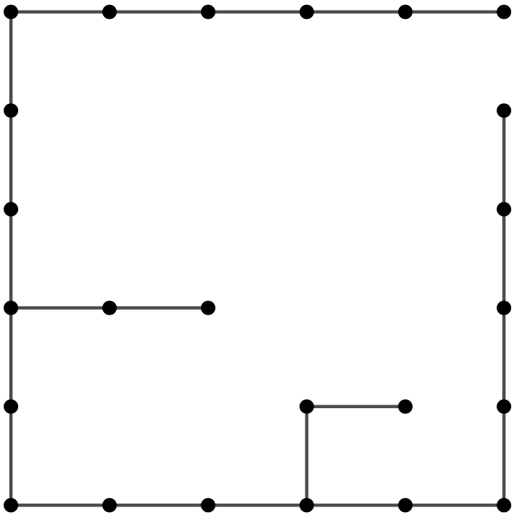
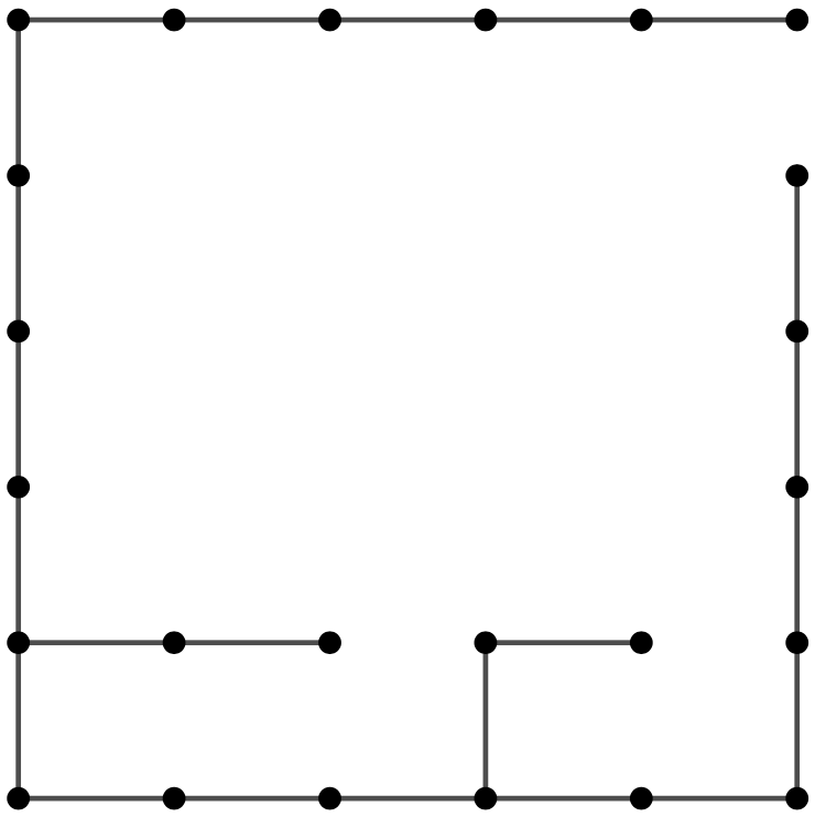
Figure 3. Dendrites $T^{1}$ (left) and $T^{2}$ (right) for $n=6$.

For each $i\in\{1,2\}$ define combinatorial graphs $G^{i}=(V^{i},E^{i})$ by

$$V^{i}:=\{\psi_{j}^{i}({\bf 0}):j\in\mathcal{A}_{n}\}\qquad\text{and}\qquad E^{i}:=\{\{p,q\}:p,q\in V^{i},[p,q]\subset T^{i}\}.$$

Note that $T^{i}=\text{Im}(G^{i})$. Next, we define a sequence of sets $(T_{m})_{m\geq 0}$ by $T_{0}=\{{\bf 0}\}$, and for any integer $m\geq 0$,

$$T_{m+1}=T_{m}\cup\left(\bigcup_{w\in\mathcal{A}_{n}^{m}}\phi_{w}^{\eta}(T^{\eta(w)})\right).$$

Define also for $m\geq 0$ the combinatorial graph $G_{m}=(V_{m},E_{m})$ via

$$V_{m}=\{\phi_{w}^{\eta}({\bf 0}):w\in\mathcal{A}_{n}^{m}\}\qquad\text{and}\qquad E_{m}=\{\{p,q\}:p,q\in V_{m},[p,q]\subset T_{m}\}.$$

Lemma 6.3.

The sequence of sets $(T_{m})_{m=0}^{\infty}$ is a nested sequence of dendrites contained in $K^{\eta}$. Moreover, for every $m\in\mathbb{N}$, a vertex $u\in V_{m}$ is a leaf of $T_{m}$ if and only if $u$ has no edges emanating to the right or upward in $T_{m}$.

Proof.

By the arguments in the proof of Lemma 4.3, for each $w\in\mathcal{A}_{n}^{*}$ we have that $\phi_{w}^{\eta}(\partial[0,1]^{2})\subset K^{\eta}$. Therefore,

$$T_{m}\subset\bigcup_{w\in\mathcal{A}_{n}^{m}}\phi_{w}^{\eta}(\partial[0,1]^{2})\subset K^{\eta}.$$

Next, we show that each $T_{m}$ is a dendrite by induction on $m$. The set $T_{0}=\{{\bf 0}\}$ is clearly a dendrite. Now assume that $T_{m}$ is a dendrite for some $m\geq 0$. We make three observations. First, by Lemma 6.2, $\phi_{w}^{\eta}(T^{\eta(w)})$ is a dendrite for any $w\in\mathcal{A}_{n}^{m+1}$. Second, by Lemma 4.2 and by Lemma 6.2, if $v,w\in\mathcal{A}_{n}^{m+1}$ are distinct, then

$$\phi_{w}^{\eta}(T^{\eta(w)})\cap\phi_{v}^{\eta}(T^{\eta(v)})\subset\phi_{w}^{\eta}([0,1)^{2})\cap\phi_{v}^{\eta}([0,1)^{2})=\emptyset.$$

Third, for any $w\in\mathcal{A}_{n}^{m+1}$ we have that $\phi_{w}^{\eta}(T^{\eta(w)})\cap T_{m+1}$ is either $\phi_{w}^{\eta}(\{0\}\times[0,1-\tfrac{1}{n}])$, or $\phi_{w}^{\eta}([0,1-\tfrac{1}{n}]\times\{0\})$, or the union of the latter two sets. In either case, $\phi_{w}^{\eta}(T^{\eta(w)})\cap T_{m+1}$ is an arc. Write now $T_{m+1}=T_{m}\cup\bigcup_{k=1}^{N}X_{k}$ where $X_{1},\dots,X_{N}$ are the components of the closure of $T_{m+1}\setminus T_{m}$. Note the sets $X_{k}$ are pairwise disjoint, by the first and second observation each $X_{k}$ is a dendrite, and by the first and third observation, $X_{i}\cap T_{m}$ is a point. Applying Lemma 2.1, we conclude that $T_{m+1}$ is a dendrite.

Finally, we prove the claim about the leaves of $T_{m}$ by induction on $m$. For $m=1$, we note that the leaves of $T^{1}$ are exactly the points $(1-\frac{1}{n},1-\frac{1}{n})$, $(1-\frac{1}{n},1-\frac{2}{n})$, $(\frac{2}{n},\frac{2}{n})$, $(1-\frac{2}{n},\frac{1}{n})$ for which it is easy to check the claim. Similarly for $T^{2}$.

Suppose now that the claim holds for some $m\in\mathbb{N}$ and let $u\in V_{m+1}$ be a vertex. Then there is a unique word $w\in\mathcal{A}_{n}^{m}$ so that $u\in\phi_{w}^{\eta}(T^{\eta(w)})$, and $u$ is a leaf in $T_{m+1}$ if and only if $(\phi_{w}^{\eta})^{-1}(u)$ is a leaf in $T^{\eta(w)}$, which is a leaf if and only if it has no edges in $T^{\eta(w)}$ emanating to the right or upward. This holds if and only if $u$ has no edges emanating upward or to the right in $T_{m+1}$. ∎

Note that for each integer $m\geq 0$,

$$T_{m}=\text{Im}(G_{m})=V_{m}\cup(\bigcup\limits_{\{p,q\}\in E_{m}}(p,q)),$$

so when we refer to a “vertex” of $T_{m}$ we mean a point $p\in V_{m}$, and when we refer to an “edge $(p,q)$ of $T_{m}$” we mean the open segment $(p,q)$ in $\mathbb{R}^{2}$ associated with the edge $\{p,q\}\in E_{m}$. Set

$$e_{b}=(0,1)\times\{0\}\qquad\text{and}\qquad e_{l}=\{0\}\times(0,1),$$

the bottom and left, respectively, open edges of $(0,1)^{2}$. Note that if $e\subset T_{m}$ is an edge in $T_{m}$, then $e$ is parallel to either the $x$-axis or to the $y$-axis, as this is true for $T^{1}$ and $T^{1}$ and the maps $\psi_{j}^{i}$ are all rotation-free and reflection-free similarities.

Lemma 6.4.

For each $m\in\mathbb{N}$, if $(p,q)$ is an edge of $T_{m}$, then there exists $w\in\mathcal{A}_{n}^{m}$ such that either $(p,q)=\phi_{w}^{\eta}(e_{b})$ or $(p,q)=\phi_{w}^{\eta}(e_{l})$.

Proof.

We proceed by induction on $m$. For $m=1$, the result follows by simple inspection, as either $T_{1}=T^{1}$ or $T_{1}=T^{2}$. Now assume the result holds for some integer $m\geq 1$. Let $(p,q)\subset T_{m+1}$ be an edge. Then there exist words $u,v\in\mathcal{A}_{n}^{m+1}$ so that $p=\phi_{u}^{\eta}({\bf 0}$ and $q=\phi_{v}^{\eta}({\bf 0}$. If there is a word $w\in\mathcal{A}_{n}^{m}$ so that $(p,q)\subset\phi_{w}^{\eta}(T^{\eta(w)})$, then there is some edge $e\subset T^{\eta(w)}$ so that $(p,q)=\phi_{w}^{\eta}(e)$, and the result follows from the $m=1$ case and from the definition of $\phi_{w}^{\eta}$. If there is no such word $w$, then we have that $(p,q)\subset T_{m}$. Since the only nondegenerate line segments contained in $T_{m}$ are contained in its edges, there is some edge $e\subset T_{m}$ so that $(p,q)\subset e$, and since $(p,q)$ is not a subset of $\phi_{v}^{\eta}(T^{\eta(v)})$ for any $v\in\mathcal{A}_{n}^{m}$, we have that $[p,q]$ is not a subset of $\phi_{v}^{\eta}([0,1)^{2})$ for any $v\in\mathcal{A}_{n}^{m}$. Then by the induction hypothesis there is some word $w\in\mathcal{A}^{m}_{n}$ so that $e=\phi_{w}^{\eta}(e_{b})$ or $e=\phi_{w}^{\eta}(e_{l})$. Note that the length of $(p,q)$ is $n^{-m-1}$, that $[p,q]\subset\phi_{w}^{\eta}([0,1]^{2})$, and that $(p,q)\subset\phi_{w}^{\eta}([0,1)^{2})$. Then either $p$ or $q$ is $\phi_{w}^{\eta}((0,1))$ or $\phi_{w}^{\eta}((1,0))$ since the edge $e$ is equal to either $\phi_{w}^{\eta}(e_{b})$ or to $\phi_{w}^{\eta}(e_{l})$. Then there is some character $j\in\mathcal{A}_{n}$ so that the other of $p$ and $q$ is equal to $\phi_{wj}^{\eta}({\bf 0}$, so $\phi_{wj}^{\eta}(e_{b})=(p,q)$ or $\phi_{wj}^{\eta}(e_{l})=(p,q)$.

∎

In the next lemma we construct intermediate parametrizations $f_{m}:[0,1]\to T_{m}$.

Lemma 6.5.

There exist a sequence of piecewise linear continuous surjections $(f_{m}:[0,1]\to T_{m})_{m\geq 0}$, a sequence $(\mathscr{N}_{m})_{m\geq 0}$ of families of nondegenerate closed intervals contained in $[0,1]$, a sequence $(\mathscr{E}_{m})_{m\geq 0}$ of families of open intervals in $[0,1]$, another sequence $(\mathscr{F}_{m})_{m\geq 0}$ of families of nondegenerate closed intervals in $[0,1]$, and a sequence of functions $(\operatorname{{\bf w}}_{m}:\mathscr{N}_{m}\to\mathcal{A}_{n}^{m})_{m\geq 0}$ satisfying the following properties.

1. For each $m\geq 0$, $\operatorname{{\bf w}}_{m}$ is a bijection between $\mathscr{N}_{m}$ and $\mathcal{A}^{m}_{n}$.

2. For each $m\geq 0$, the families $\mathscr{E}_{m},\mathscr{N}_{m},\mathscr{F}_{m}$ are pairwise disjoint and the elements of $\mathscr{E}_{m}\cup\mathscr{N}_{m}\cup\mathscr{F}_{m}$ are pairwise disjoint. Moreover, $[0,1]=\bigcup(\mathscr{E}_{m}\cup\mathscr{N}_{m}\cup\mathscr{F}_{m})$.

3. For each $m\geq 0$ and $J\in\mathscr{E}_{m}$, there exists $w\in\mathcal{A}_{n}^{m}$ such that $f_{m}|J$ is a linear bijection onto either $\phi^{\eta}_{w}(e_{b})$ or $\phi^{\eta}_{w}(e_{l})$, and there exists a unique interval $J^{\prime}\in\mathscr{E}_{m}\setminus\{J\}$, so that $f_{m}|J^{\prime}=(f_{m}|J)\circ\zeta_{J^{\prime}}$ where $\zeta_{J^{\prime}}:J^{\prime}\to J$ is the unique linear orientation reversing map. Furthermore, $f_{m+1}(J)\subset\phi^{\eta}_{w}([0,1)^{2})$. Conversely, if $(p,q)$ is an edge of $T_{m}$, then there exist exactly two intervals $J,J^{\prime}\in\mathscr{E}_{m}$ such that $f_{m}(J)=f_{m}(J^{\prime})=(p,q)$.

4. For each $m\geq 0$ and $I\in\mathscr{N}_{m}$, $f_{m}|I$ is constant equal to $\phi^{\eta}_{\operatorname{{\bf w}}_{m}(I)}({\bf 0}$. Conversely, $f_{m}(\bigcup\mathscr{N}_{m})=V_{m}$. Moreover, $f_{m+1}(I)\subset\phi^{\eta}_{\operatorname{{\bf w}}_{m}(I)}([0,1)^{2})$.

5. For each $m\geq 0$ and $I\in\mathscr{F}_{m}$, $f_{m}|I$ is constant and $f_{m}(I)\in V_{m}$. Furthermore, $f_{m+1}|I=f_{m}|I$.

6. For each $m\geq 0$ and $J\in\mathscr{E}_{m+1}\cup\mathscr{N}_{m+1}$, there exists $I\in\mathscr{E}_{m}\cup\mathscr{N}_{m}$ such that $J\subset I$. Moreover, if $J\in\mathscr{N}_{m+1}$ and $I\in\mathscr{N}_{m}$ with $J\subset I$, then $\operatorname{{\bf w}}_{m}(I)=\operatorname{{\bf w}}_{m+1}(J)(m)$.

7. For each $m\geq 0$ and $J\in\mathscr{E}_{m}$, there exists $I\in\mathscr{N}_{m+1}$ such that $I\subset J$ and $f_{m+1}(I)$ is a leaf in $T_{m+1}$.

Proof.

We start by defining two pairs of preliminaries maps.

First, fix for each $i\in\{1,2\}$ a continuous surjection $\tau_{i}:[0,1]\to T^{i}$ with the following properties.

1. The map $\tau_{i}$ is a 2–to–1 tour of the edges of $T^{i}$ and is linear along edges with $\tau_{i}(0)=\tau_{i}(1)={\bf 0}$.

2. For every vertex $v\in V^{i}$ other than ${\bf 0}$, the preimage $\tau_{i}^{-1}(\{v\})$ has a number of components equal to the valence of the vertex $v$ and each component is a nondegenerate closed interval.

3. The preimage $\tau_{i}^{-1}(\{{\bf 0}\})$ is made up of three disjoint nondegenerate closed intervals.

4. There exists $t_{i}$ in the component of $\tau_{i}^{-1}(\{{\bf 0}\})$ which does not contain $0$ or $1$ such that $\tau_{i}^{-1}(\{(0,1-1/n)\})$ lies to the left of $t_{i}$ and $\tau_{i}^{-1}(\{(1-1/n,0)\})$ lies to the right of $t_{i}$.

Next, for each $i\in\{1,2\}$, define the combinatorial tree $\tilde{G}^{i}=(\tilde{V}^{i},\tilde{E}^{i})$ via

$$\tilde{V}^{i}:=V^{i}\cup\{(1,0),(0,1)\},\quad\tilde{E}^{i}=E^{i}\cup\{\{(1-1/n,0),(1,0)\},\{(0,1-1/n),(0,1)\}\},$$

and let $\tilde{T}^{i}:=\text{Im}(\tilde{G}^{i})$. As in the previous paragraph, it is easy to see that for each $i\in\{1,2\}$ there exists a continuous surjection $\tilde{\tau}_{i}:[0,1]\to\tilde{T}^{i}$ with the following properties.

1. The map $\tilde{\tau}_{i}$ is a 2–to–1 tour of the edges of $\tilde{T}^{i}$ and is linear along edges with $\tilde{\tau}_{i}(0)=\tilde{\tau}_{i}(1)={\bf 0}$.

2. For every vertex $v\in\tilde{V}^{i}$ other than ${\bf 0}$, $(0,1)$, and $(1,0)$, the preimage $\tilde{\tau}_{i}^{-1}(\{v\})$ has a number of components equal to the valence of the vertex $v$ and each component is a nondegenerate closed interval.

3. The preimage $\tilde{\tau}_{i}^{-1}(\{{\bf 0}\})$ is made up of three disjoint nondegenerate closed intervals.

4. The preimages $\tilde{\tau}_{i}^{-1}(\{(1,0)\})$ and $\tilde{\tau}_{i}^{-1}(\{(0,1)\})$ are both singletons, denoted by $s_{i,U}$ and $s_{i,L}$, respectively.

5. There exists $\tilde{t}_{i}$ in the component of $\tilde{\tau}_{i}^{-1}(\{{\bf 0}\})$ which does not contain $0$ or $1$ such that $s_{i,U}$ lies to the left of $\tilde{t}_{i}$ and $s_{i,L}$ lies to the right of $\tilde{t}_{i}$.

6. There are disjoint nondegenerate closed intervals $I_{i,1},I_{i,2},I_{i,3},I_{i,4}\subset[0,1]$, denoted by $I_{i,j}=[a_{i,j},b_{i,j}]$, $j=1,\dots,4$ equal to the preimages of the four leaves of $T^{i}$, so that

   $$0<a_{i,1}<s_{i,U}<a_{i,2}<\tilde{t}_{i}<a_{i,3}<s_{i,L}<a_{i,4}<b_{i,4}<1.$$

Let $T$ be one of the trees $T^{i}$ or $\tilde{T}^{i}$ above, let $V$ and $E$ be the corresponding vertex and edge sets, respectively, and let $\tau:[0,1]\to T$ be the map defined above corresponding to $T$.

• Define $\mathcal{E}(\tau)$ to be the set of components of preimages of open edges in $E$.

• If $\tau\in\{\tau_{1},\tau_{2}\}$, then for each $v\in V$ choose a nondegenerate component $I_{v}$ of the preimage $\tau^{-1}(\{v\})$ and let $\mathscr{N}(\tau)=\{I_{v}:v\in V\}$.

• If instead $\tau\in\{\tilde{\tau}_{1},\tilde{\tau}_{2}\}$, then for a vertex $v\in V$ that is not a leaf, choose a nondegenerate component $I_{v}$ of the preimage $\tau^{-1}(\{v\})$, and for each vertex $v\in V$ that is a leaf other than $(1,0)$ or $(0,1)$, let $I_{v}=I_{i,j}$ where $j\in\{1,2,3,4\}$ is chosen so that $\tau(I_{i,j})=v$. We then define $\mathscr{N}(\tau)=\{I_{v}:v\in V\setminus\{(1,0),(0,1)\}\}$.

• Define $\mathcal{F}(\tau)$ to be the set of nondegenerate components of preimages under $\tau$ of vertices in $T$ which are not already in $\mathcal{N}(\tau)$.

The construction of maps $f_{m}$ and families $\mathscr{E}_{m},\mathscr{F}_{m},\mathscr{N}_{m}$ is done in an inductive fashion.

Set $f_{0}:[0,1]\to T_{0}$ to be the constant map $f_{0}\equiv{\bf 0}$, set $\mathscr{N}_{0}=\{[0,1]\}$, $\mathscr{E}_{0}=\emptyset$, $\mathscr{F}_{0}=\emptyset$, and set $\operatorname{{\bf w}}_{0}([0,1])=\varepsilon$. Properties (P1)–(P7) are all either clear or vacuous for $m=0$.

Assume now that for some $m\geq 0$ we have constructed the map $f_{m}$, families $\mathscr{E}_{m},\mathscr{F}_{m}$, and $\mathscr{N}_{m}$, and bijection $\operatorname{{\bf w}}_{m}:\mathscr{N}_{m}\to\mathcal{A}_{n}^{m}$ satisfying (P1)–(P7). For elements $I\in\mathscr{E}_{m}\cup\mathscr{N}_{m}$, we will define the collections $\mathscr{E}_{m+1}(I),\mathscr{N}_{m+1}(I)$, and $\mathscr{F}_{m+1}(I)$. We then set

$$\mathscr{E}_{m+1} =\bigcup_{I\in\mathscr{E}_{m}\cup\mathscr{N}_{m}}\mathscr{E}_{m+1}(I),$$

$$\mathscr{N}_{m+1} =\bigcup_{I\in\mathscr{E}_{m}\cup\mathscr{N}_{m}}\mathscr{N}_{m+1}(I),$$

$$\mathscr{F}_{m+1} =\mathscr{F}_{m}\cup\bigcup_{I\in\mathscr{E}_{m}\cup\mathscr{N}_{m}}\mathscr{F}_{m+1}(I).$$

Intervals in $\mathscr{F}_{m}$. If $I\in\mathscr{F}_{m}$, then set $f_{m+1}|I=f_{m}$.

Intervals in $\mathscr{E}_{m}$. Let $I\in\mathscr{E}_{m}$ and write $I=(a,b)$. By (P3) there exists $I^{\prime}=(a^{\prime},b^{\prime})\in\mathscr{E}_{m}\setminus\{I\}$ such that $f_{m}|I^{\prime}=(f_{m}|I)\circ\zeta_{I^{\prime}}$ where $\zeta_{I^{\prime}}:I^{\prime}\to I$ is the unique linear orientation reversing map and there exists a word $v\in\mathcal{A}_{n}^{m}$ so that $f_{m}(I)=\phi_{v}^{\eta}(e_{b})$ or $f_{m}(I)=\phi_{v}^{\eta}(e_{l})$. If $f_{m}(I)=\phi^{\eta}_{v}(e_{l})$, then, without loss of generality, we may assume that the $y$-coordinate of $f_{m}$ is increasing inside $I$ and decreasing inside $I^{\prime}$. Let $\tilde{\theta}_{I}:I\to(0,s_{\eta(v),U})$ be linear, bijective, and increasing, and let $\tilde{\xi}_{I^{\prime}}:I^{\prime}\to(s_{\eta(v),U},\tilde{t}_{\eta(v)})$ be linear, bijective, and decreasing. We define

$$f_{m+1}|I=\phi_{v}^{\eta}\circ\tilde{\tau}_{\eta(v)}\circ\tilde{\theta}_{I}\qquad\text{and}\qquad f_{m+1}|I^{\prime}=\phi_{v}^{\eta}\circ\tilde{\tau}_{\eta(v)}\circ\tilde{\xi}_{I^{\prime}}.$$

Define $\mathscr{E}_{m+1}(I)=\{\tilde{\theta}_{I}^{-1}(J):J\in\mathcal{E}(\tilde{\tau}_{\eta(v)})\}$ and $\mathscr{E}_{m+1}(I^{\prime})=\{\tilde{\xi}_{I^{\prime}}^{-1}(J):J\in\mathcal{E}(\tilde{\tau}_{\eta(v)})\}$. We define $\mathscr{N}_{m+1}(I)$, $\mathscr{N}_{m+1}(I^{\prime})$, $\mathscr{F}_{m+1}(I)$, and $\mathscr{F}_{m+1}(I^{\prime})$ in a similar manner. If $f_{m}(I)=\phi^{\eta}_{v}(e_{b})$, then we proceed in a similar manner, interchanging $s_{\eta(v),U}$ with $s_{\eta(v),L}$ above.

If $J\in\mathscr{N}_{m+1}(I)$, then there is a character $j\in\mathcal{A}_{n}$ so that $f_{m+1}(J)=\phi_{vj}^{\eta}({\bf 0}$, and we define $\operatorname{{\bf w}}_{m+1}(I)=vj$. Note that if $J,Q\in\mathscr{N}_{m+1}(I)\cup\mathscr{N}_{m+1}(I^{\prime})$ are distinct, then $\operatorname{{\bf w}}_{m+1}(J)\neq\operatorname{{\bf w}}_{m+1}(Q)$ as $\tilde{\theta}_{I}(J)\neq\tilde{\theta}_{I}(Q)$ are distinct intervals in, for example, $\mathcal{N}(\tilde{\tau}_{\eta(v)})$ ($\tilde{\theta}_{I}$ may be $\tilde{\xi}_{I^{\prime}}$ instead).

Intervals in $\mathscr{N}_{m}$. Let $I\in\mathscr{N}_{m}$ and write $I=[a,b]\subset[0,1]$. We consider four cases.

Case 1. If the vertex $f_{m}(I)$ in $T_{m}$ has an edge in $T_{m}$ emanating to the right and no edge emanating upward, then define $\zeta_{I}:I\to[0,t_{\eta(\operatorname{{\bf w}}_{m}(I))}]$ to be the unique linear increasing bijection, and let

$$f_{m+1}|I=\phi^{\eta}_{\operatorname{{\bf w}}_{m}(I)}\circ\tau_{\eta(\operatorname{{\bf w}}_{m}(I))}\circ\zeta_{I}.$$

Define $\mathscr{F}_{m+1}(I),\mathscr{E}_{m+1}(I),\mathscr{N}_{m+1}(I)$ in a manner similar to those for $I\in\mathscr{E}_{m}$ above.

Case 2. If the vertex $f_{m}(I)$ in $V_{m}$ has an edge in $T_{m}$ emanating upward and no edge emanating to the right, then define $\xi_{I}:I\to[t_{\eta(\operatorname{{\bf w}}(I))},1]$ to be the unique increasing linear bijection, and let

$$f_{m+1}|I=\phi^{\eta}_{\operatorname{{\bf w}}_{m}(I)}\circ\tau_{\eta(\operatorname{{\bf w}}_{m}(I))}\circ\xi_{I}.$$

Define $\mathscr{F}_{m+1}(I),\mathscr{E}_{m+1}(I),\mathscr{N}_{m+1}(I)$ in a manner similar to those for $I\in\mathscr{E}_{m}$ above.

Case 3. If the vertex $f_{m}(I)$ is a leaf in $T_{m}$, then let $\sigma_{I}:I\to[0,1]$ be the unique increasing linear bijection, and let

$$f_{m+1}|I=\phi^{\eta}_{\operatorname{{\bf w}}_{m}(I)}\circ\tau_{\eta(\operatorname{{\bf w}}_{m}(I))}\circ\sigma_{I}.$$

Define $\mathscr{F}_{m+1}(I),\mathscr{E}_{m+1}(I),\mathscr{N}_{m+1}(I)$ in a manner similar to those for $I\in\mathscr{E}_{m}$ above.

Case 4. If the vertex $f_{m}(I)$ has an edge in $T_{m}$ emanating upward and another edge emanating to the right, then simply set $f_{m+1}|I=f_{m}|I$ and let $\mathscr{N}_{m+1}(I)=\{I\}$, $\mathscr{E}_{m+1}(I)=\emptyset$, and $\mathscr{F}_{m+1}(I)=\emptyset$.

By definition of $\tau_{\eta(\operatorname{{\bf w}}_{m}(I))}$, for any $Q\in\mathscr{N}_{m+1}(I)$, there is a character $j\in\mathcal{A}_{n}$ so that $f_{m+1}(Q)=\{\phi^{\eta}_{\operatorname{{\bf w}}_{m}(I)j}({\bf 0}\}$, and we set $\operatorname{{\bf w}}_{m+1}(Q)=\operatorname{{\bf w}}_{m}(I)j$.

We now prove (P1)–(P7) for $f_{m+1}$, $\mathscr{E}_{m+1}$, $\mathscr{N}_{m+1}$, $\mathscr{F}_{m+1}$, and $\operatorname{{\bf w}}_{m+1}$.

We start with (P2). Since (P2) holds for $\mathscr{E}_{m},\mathscr{N}_{m}$, and $\mathscr{F}_{m}$, and since intervals in $\mathscr{F}_{m+1}$ are not partitioned, it suffices to show that for every $I\in\mathscr{E}_{m}\cup\mathscr{N}_{m}$, the families $\mathscr{E}_{m+1}(I),\mathscr{N}_{m+1}(I)$, and $\mathscr{F}_{m+1}(I)$ are pairwise disjoint with disjoint elements covering $I$. If $I\in\mathscr{E}_{m}$, then this holds by definitions of $\mathcal{E}(\tilde{\tau}_{i})$, $\mathcal{N}(\tilde{\tau}_{i})$, and $\mathcal{F}(\tilde{\tau}_{i})$. If $I\in\mathscr{N}_{m}$, then this follows from the definitions of $\mathcal{E}(\tau_{i})$, $\mathcal{N}(\tau_{i})$, and $\mathcal{F}(\tau_{i})$.

The first part of (P3) follows from the analogous properties defining $\tilde{\tau}_{i}$. The converse part of (P3) follows from (P3) and (P6) at $m$ and by the definitions of $\tilde{\tau}_{i}$ and $\tau_{i}$.

The first part of (P4) follows from design of $\mathcal{N}(\tau_{i})$ and $\mathcal{N}(\tilde{\tau}_{i})$ along with (P1) and (P4) at $m$. The converse part follows from (P1), (P3), (P4), and (P6) at $m$ along with design of $\tau_{i}$ and $\tilde{\tau}_{i}$.

Property (P5) follows immediately from the definitions of $\mathcal{F}(\tau_{i})$ and $\mathcal{F}(\tilde{\tau}_{i})$.

The first part of (P6) follows from (P2) at $m$, as for every $I\in\mathscr{E}_{m}\cup\mathscr{N}_{m}$ and every $J\in\mathscr{E}_{m+1}(I)\cup\mathscr{N}_{m+1}(I)$, $J\subset I$, while every $J\in\mathscr{E}_{m+1}\cup\mathscr{N}_{m+1}$ is in $\mathscr{E}_{m+1}(I)\cup\mathscr{N}_{m+1}(I)$ for some $I\in\mathscr{E}_{m}\cup\mathscr{N}_{m}$. The converse part of (P6) is immediate from the definition of $\operatorname{{\bf w}}_{m+1}(J)$ for $J\in\mathscr{N}_{m+1}(I)$ with $I\in\mathscr{N}_{m}$.

Property (P7) follows from properties (4), (5), and (6) in the definition of $\tilde{\tau}_{i}$.

Finally, we verify (P1). We first show that $\operatorname{{\bf w}}_{m+1}$ is injective. Let $I,J\in\mathscr{N}_{m+1}$ be distinct intervals. Then by (P6), let $\tilde{I},\tilde{J}\in\mathscr{E}_{m}\cup\mathscr{N}_{m}$ so that $I\in\mathscr{N}_{m+1}(\tilde{I}),J\in\mathscr{N}_{m+1}(\tilde{J})$. If $\tilde{I}=\tilde{J}$ are the same element of $\mathscr{E}_{m}$, then $\operatorname{{\bf w}}_{m+1}(I)\neq\operatorname{{\bf w}}_{m+1}(J)$ by definitions of $\mathcal{N}(\tilde{\tau}_{i})$. If $\tilde{I}=\tilde{J}$ are the same element of $\mathscr{N}_{m}$, then by (P6) there are characters $i,j\in\mathcal{A}_{n}$ with $\operatorname{{\bf w}}_{m+1}(I)=\operatorname{{\bf w}}_{m}(\tilde{I})i$, $\operatorname{{\bf w}}_{m+1}(J)=\operatorname{{\bf w}}_{m}(\tilde{I})j$. Then by the definitions of $\mathcal{N}(\tau_{i})$, we have that $i\neq j$. If $\tilde{I}\neq\tilde{J}$ are distinct intervals, both in $\mathscr{N}_{m}$, then by (P6) at $m+1$ and (P1) at $m$, we have that $\operatorname{{\bf w}}_{m+1}(I)(m)\neq\operatorname{{\bf w}}_{m+1}(J)(m)$, so $\operatorname{{\bf w}}_{m+1}(I)\neq\operatorname{{\bf w}}_{m+1}(J)$. If $\tilde{I}\neq\tilde{J}$ with $\tilde{J}\in\mathscr{E}_{m}$ and $\tilde{I}\in\mathscr{N}_{m}$, then by definitions of $\tau_{i}$ and $\tilde{\tau}_{i}$, $f_{m+1}(\tilde{I})\cap f_{m+1}(\tilde{J})=\emptyset$, so by (P3) and (P4), $\operatorname{{\bf w}}_{m+1}(I)\neq\operatorname{{\bf w}}_{m+1}(J)$. Similarly $\operatorname{{\bf w}}_{m+1}(I)\neq\operatorname{{\bf w}}_{m+1}(J)$ if $\tilde{I}\neq\tilde{J}$ with $\tilde{J}\in\mathscr{E}_{m}$ and $\tilde{I}\in\mathscr{E}_{m}\setminus\{\tilde{J},\tilde{J}^{\prime}\}$. If $\tilde{J}\in\mathscr{E}_{m}$ and $\tilde{I}=\tilde{J}^{\prime}$, then $\operatorname{{\bf w}}_{m+1}(I)\neq\operatorname{{\bf w}}_{m+1}(J)$ by definition of $\mathcal{N}(\tilde{\tau}_{i})$.

To conclude the proof, we show that $\operatorname{{\bf w}}_{m+1}:\mathscr{N}_{m+1}\to\mathcal{A}_{n}^{m+1}$ is surjective. Let $u\in\mathcal{A}_{n}^{m+1}$ be a word. By (P1) at $m$, there exists a unique interval $I\in\mathscr{N}_{m}$ so that $\operatorname{{\bf w}}_{m}(I)=u(m)$. If $f_{m}(I)$ is a leaf in $T_{m}$, then by definition of $\mathcal{N}(\tau_{i})$, for each $j\in\mathcal{A}_{n}$ there is an interval $J\in\mathscr{N}_{m+1}(I)$ so that $\operatorname{{\bf w}}_{m+1}(J)=\operatorname{{\bf w}}_{m+1}(I)j$, in particular one of them has $\operatorname{{\bf w}}_{m+1}(J)=u$. If $f_{m}(I)$ is not a leaf in $T_{m}$, then the result follows by definitions of $\mathcal{N}(\tilde{\tau}_{i})$ and $\mathcal{N}(\tau_{i})$ as well as (P3) at $m$. ∎

Define now the map $\operatorname{{\bf w}}:\bigcup_{m=0}^{\infty}\mathscr{N}_{m}\to\mathcal{A}_{n}^{*}$ by $\operatorname{{\bf w}}(I)=\operatorname{{\bf w}}_{m}(I)$ if $I\in\mathscr{N}_{m}$. By (P1) of Lemma 6.5 we have that $\operatorname{{\bf w}}$ is a well-defined bijection.

Corollary 6.6.

The maps $(f_{m})_{m\geq 0}$ of Lemma 6.5 converge uniformly to a continuous surjection $f:[0,1]\to K^{\eta}$.

Proof.

Since $T_{m}\subset K^{\eta}$, the Hausdorff distance

$$\operatorname{dist}_{H}(T_{m},K^{\eta})\leq\operatorname{dist}_{H}(V_{m},K^{\eta})\leq\max_{w\in\mathcal{A}^{m}_{n}}\operatorname{diam}{K_{w}^{\eta}}\leq n^{-m}\sqrt{2}.$$

Therefore, $\overline{\bigcup_{m\in\mathbb{N}}T_{m}}=K^{\eta}$, as $K^{\eta}$ is compact.

Next we claim that for every $m\in\mathbb{N}$,

(6.1) $$\|f_{m}-f_{m+1}\|_{\infty}\leq n^{-m}\sqrt{2}.$$

Fix $m\in\mathbb{N}$ and $x\in[0,1]$. By Lemma 6.5(P1), there exists $I\in\mathscr{N}_{m}\cup\mathscr{E}_{m}\cup\mathscr{F}_{m}$ so that $x\in I$. If $I\in\mathscr{F}_{m}$, then by Lemma 6.5(P5) we have that $f_{m}(x)=f_{m+1}(x)$. If $I\in\mathscr{N}_{m}$, then by Lemma 6.5(P4) we have that $f_{m}(x),f_{m+1}(x)\in\phi^{\eta}_{\operatorname{{\bf w}}(I)}([0,1]^{2})$. Finally, if $I\in\mathscr{E}_{m}$, then by Lemma 6.5(P3) we have that there is some word $v\in\mathcal{A}_{n}^{m}$ such that $f_{m}(x),f_{m+1}(x)\in\phi^{\eta}_{v}([0,1]^{2})$. In any case, we have the claimed estimate.

Hence, the functions $f_{m}$ converge uniformly to a continuous map $f:[0,1]\to[0,1]^{2}$. Furthermore, because the dendrites $T_{m}\subset K^{\eta}$ are nested and $f_{m}:[0,1]\to T_{m}$ are surjective, we have that the uniform limit $f$ is a continuous parametrization of $K^{\eta}$, as desired. ∎

Lemma 6.7.

For each $m\in\mathbb{N}$ and every pair of distinct intervals $I,J\in\mathscr{E}_{m}\cup\mathscr{N}_{m}$, we have that $\mathcal{H}^{\alpha_{n}}(f(I)\cap f(J))=0$.

Before proving the lemma we recall the well-known definition of porosity. Given a metric space $X$, we say that a set $Y\subset X$ is porous in $X$ if there exists $c>1$ such that for any $r<\operatorname{diam}{X}$ and any $x\in X$, there exists $y\in B(x,r)$ such that $B(y,c^{-1}r)\subset B(x,r)\setminus Y$.

Proof.

We claim that $f(I)\cap f(J)$ is porous in $K^{\eta}$. Assuming the claim, since $K^{\eta}$ is Ahlfors $\alpha_{n}$-regular by Proposition 5.1, it follows from [BHR01, Lemma 3.12] that the Hausdorff dimension (in fact, the Assouad dimension) of $f(I)\cap f(J)$ is less than $\alpha_{n}$ which gives the lemma.

To prove porosity, note first that by Lemma 6.5 (P3), (P4), and (P6) there exists a word $v\in\mathcal{A}_{n}^{m}$ such that $f(I)\cap f(J)\subset K^{\eta}_{v}$. Fix $x\in K^{\eta}$ and $r\in(0,n^{-m}]$. There exists an integer $k_{0}\in\mathbb{N}$ such that $n^{-k_{0}}\leq r<n^{-k_{0}+1}$, and so there exists $w\in\mathcal{A}_{n}^{k_{0}+1}$ with $K^{\eta}_{w}\subset\overline{B}(x,r)\cap K^{\eta}$.

We now prove that there are characters $i,j\in\mathcal{A}_{n}$ such that $f(I)\cap f(J)\cap K^{\eta}_{wji}=\emptyset$. This falls to a case study.

Case 1. Suppose that $I,J\in\mathscr{N}_{m}$. Then $f(I)\cap\phi^{\eta}_{\operatorname{{\bf w}}(J)}((0,1)^{2})=\emptyset$ and $f(J)\cap\phi^{\eta}_{\operatorname{{\bf w}}(I)}((0,1)^{2})=\emptyset$ by Lemma 4.2, Lemma 6.5(P4), and the fact that $\operatorname{{\bf w}}(I),\operatorname{{\bf w}}(J)$ are distinct words of length $m$. Moreover, at least one of $\phi^{\eta}_{w}((0,1)^{2})\cap\phi^{\eta}_{\operatorname{{\bf w}}(I)}([0,1]^{2})$ and $\phi^{\eta}_{w}((0,1)^{2})\cap\phi^{\eta}_{\operatorname{{\bf w}}(J)}([0,1]^{2})$ is empty, so since there are characters $i,j\in\mathcal{A}_{n}$ for which $K^{\eta}_{wji}\subset\phi^{\eta}_{w}((0,1)^{2})$, we have

$$f(I)\cap f(J)\cap K^{\eta}_{wji}=\emptyset.$$

Case 2. Suppose that at least one of $I$, $J$ is in $\mathscr{E}_{m}$. By Lemma 6.5(P3), (P4), and (P6), there exist words $u,v\in\mathcal{A}_{n}^{m}$ such that $f(J)\subset K^{\eta}_{u}$ and $f(I)\subset K^{\eta}_{v}$.

If $u\neq v$, then we proceed as in Case 1 with $u$ playing the role of $\operatorname{{\bf w}}(J)$ and $v$ playing the role of $\operatorname{{\bf w}}(I)$. If $f(I)$ or $f(J)$ is a singleton, then the existence of such characters $i,j\in\mathcal{A}_{n}$ is clear.

Therefore, we may assume for the rest of Case 2 that $u=v$ and that neither of $f(I),f(J)$ is a singleton. If $f_{k_{0}+1}(J)\cap K^{\eta}_{w}=\emptyset$, then $f(J)\cap\phi^{\eta}_{w}((0,1)^{2})=\emptyset$ by Lemma 4.2 and by Lemma 6.5 (P3), (P4), and (P5), so the existence of such characters $i,j\in\mathcal{A}_{n}$ is clear. Similarly if $f_{k_{0}+1}(I)\cap K^{\eta}_{w}=\emptyset$. Now assume that $f_{k_{0}+1}(I)\cap K^{\eta}_{w}\neq\emptyset$ and $f_{k_{0}+1}(J)\cap K^{\eta}_{w}\neq\emptyset$. Then there are distinct leaves $p_{1},p_{2}\in T_{k_{0}+2}$ with $p_{1},p_{2}\in K^{\eta}_{w}$ and distinct intervals $Q_{1},Q_{2}\in\mathscr{N}_{k_{0}+2}$ such that $Q_{1}\subset J$ and $Q_{2}\subset I$ satisfy $f_{k_{0}+2}|Q_{1}\equiv p_{1}$ and $f_{k_{0}+2}|Q_{2}\equiv p_{2}$. Then $f([0,1]\setminus Q_{1})\cap\phi^{\eta}_{\operatorname{{\bf w}}(Q_{1})}((0,1)^{2})=\emptyset$ and $\operatorname{{\bf w}}(Q_{1})(k_{0}+1)=w$, so there is a pair of characters $i,j\in\mathcal{A}_{n}$ so that $wj=\operatorname{{\bf w}}(Q_{1})$ and $K^{\eta}_{wji}\subset\phi^{\eta}_{wj}((0,1)^{2})$. Since $I,J$ are distinct, and thus disjoint, we have that $f(I)\cap\phi^{\eta}_{wj}((0,1)^{2})=\emptyset$, concluding Case 2.

Additionally, there exists a point $y\in K^{\eta}_{wji}$ with $\overline{B}(y,n^{-k_{0}-5})\cap K^{\eta}\subset K^{\eta}_{wji}$. Thus, for every $r\in(0,n^{-m}]$ and each $x\in K^{\eta}$, there exists $y\in K^{\eta}$ such that

$$\overline{B}(y,n^{-5}r)\cap K^{\eta}\subset K^{\eta}\cap(\overline{B}(x,r)\setminus(f(I)\cap f(J))).\qed$$

We are now ready to prove Proposition 6.1. Throughout this proof, when we write any of (P1)–(P7) we mean the appropriate property (P1)–(P7) from Lemma 6.5.

Proof of Proposition 6.1.

Let $f_{m}$, $\mathscr{E}_{m},\mathscr{N}_{m},\mathscr{F}_{m}$, and $\operatorname{{\bf w}}$ be as in Lemma 6.5. Note that $\bigcup_{m\geq 0}\mathscr{F}_{m}$ is a countably infinite set, and let $\{S_{1},S_{2},\dots\}$ be an enumeration of $\bigcup_{m\geq 0}\mathscr{F}_{m}$. Define an increasing homeomorphism $\zeta:[0,1]\to[0,1]$ so that for every $S_{j}\in\bigcup_{m\geq 0}\mathscr{F}_{m}$ $|\zeta(S_{j})|=2^{-j-1}$ and for every integer $m\geq 0$ and each $J\in\mathscr{E}_{m}\cup\mathscr{N}_{m}$,

$$|\zeta(J)|=\frac{1}{2}\pi_{\eta}\#\nu_{n}(f(J))+\sum_{\begin{subarray}{c}S_{j}\in\bigcup\limits_{k\geq 0}\mathscr{F}_{k}\\ S_{j}\subset J\end{subarray}}2^{-j-1},$$

where $f$ is the uniform limit of the maps $f_{m}$ from Corollary 6.6 and $\nu_{n}$ is the probability measure from §2.2. We further require that for every integer $m\geq 0$ and each $J\in\mathscr{E}_{m}$, $f_{m}\circ\zeta^{-1}$ has constant derivative on $J\setminus(\bigcup\{S_{j}:S_{j}\in\bigcup_{i\geq 0}\mathscr{F}_{i},S_{j}\subset J\})$. By Lemma 6.7, these requirements are valid, as by Proposition 5.1 $\pi_{\eta}\#\nu_{n}$ and $\mathcal{H}^{\alpha_{n}}\hbox{ {\vrule height=6.25963pt}{\leaders\hrule\hskip 5.69046pt} }K^{\eta}$ have the same null sets. Now for every $m\geq 0$, let $F_{m}$ be defined by $F_{m}=f_{m}\circ\zeta^{-1}$. Note that the maps $F_{m}$ converge uniformly to the map $F=f\circ\zeta^{-1}$.

To finish the proof it suffices to show that the function $F$ is $(1/\alpha_{n})$-Hölder continuous.

To prove this, we appeal to [BNV19, Lemma B.1], but beforehand we make a needed observation. From (P7), we have that for each $m\in\mathbb{N}$ and each $J\in\mathscr{E}_{m}$, there is some $I\in\mathscr{N}_{m+1}$ so that $F_{m+1}\circ\zeta(I)$ is a leaf in $T_{m+1}$ and $I\subset J$. Then since $F_{m+1}(\zeta(I))=\phi^{\eta}_{\operatorname{{\bf w}}(I)}((0,0))$ is a leaf in $T_{m+1}$, we have that

$$F_{m+1}(\zeta([0,1]\setminus I))\cap\phi^{\eta}_{\operatorname{{\bf w}}(I)}(T^{\eta(\operatorname{{\bf w}}(I))})=\emptyset.$$

We claim that for every integer $k\geq m+1$, $F_{k}(\zeta([0,1]\setminus I))\cap\phi_{\operatorname{{\bf w}}(I)}^{\eta}((0,1)^{2})=\emptyset$. To this end, fix an integer $k\geq m+1$ and let $t\in[0,1]\setminus I$. Note that by Lemma 4.2, it is sufficient to show that there exists a word $u\in\mathcal{A}_{n}^{m+1}$ different from $\operatorname{{\bf w}}(I)$ such that $F_{k}\circ\zeta(t)\in\phi_{u}^{\eta}([0,1]^{2})$. By (P2), let $Q\in(\mathscr{E}_{m+1}\cup\mathscr{F}_{m+1}\cup\mathscr{N}_{m+1})\setminus\{I\}$ be the unique such interval with $t\in Q$.

If $Q\in\mathscr{F}_{m+1}$, then by (P5) there exists a word $u\in\mathcal{A}_{n}^{m+1}$ so that

$$F_{k}\circ\zeta(t)=F_{m+1}\circ\zeta(t)=\phi_{u}^{\eta}({\bf 0}).$$

Then since

$$F_{m+1}(\zeta([0,1]\setminus I))\cap\phi^{\eta}_{\operatorname{{\bf w}}(I)}(T^{\eta(\operatorname{{\bf w}}(I))})=\emptyset,$$

we have that $u\neq\operatorname{{\bf w}}(I)$.

If $Q\in\mathscr{E}_{m+1}$, then by (P3) and Lemma 6.4, there exists a word $u\in\mathcal{A}_{n}^{m+1}$ so that $F_{m+1}(\zeta(Q))=\phi_{u}^{\eta}(e_{b})$ or $F_{m+1}(\zeta(Q))=\phi_{u}^{\eta}(e_{l})$. In either case, by (P3), (P4), and (P5) we have that $F_{k}(\zeta(Q))\subset\phi_{u}^{\eta}([0,1)^{2})$. Note that $\phi_{\operatorname{{\bf w}}(I)}^{\eta}(e_{l})$ emanates from $\phi_{\operatorname{{\bf w}}(I)}^{\eta}({\bf 0}$ upward and $\phi_{\operatorname{{\bf w}}(I)}^{\eta}(e_{b})$ emanates from $\phi_{\operatorname{{\bf w}}(I)}^{\eta}({\bf 0}$ to the right. Since $\phi_{\operatorname{{\bf w}}(I)}^{\eta}({\bf 0}$ is a leaf in $T_{m+1}$, by Lemma 6.3 we must have that $u\neq\operatorname{{\bf w}}(I)$.

Now if $Q\in\mathscr{N}_{m+1}\setminus\{I\}$, then by (P1), $\operatorname{{\bf w}}(Q)\neq\operatorname{{\bf w}}(I)$. By (P3), (P4), and (P5), $F_{k}(\zeta(Q))\subset\phi_{\operatorname{{\bf w}}(Q)}^{\eta}([0,1)^{2})$. Therefore, $F_{k}\circ\zeta(t)\notin\phi_{\operatorname{{\bf w}}(I)}^{\eta}((0,1)^{2})$, completing the proof of the claim.

Thus if $J\in\mathscr{E}_{m}$, then there is an interval $I\in\mathscr{N}_{m+1}$ with $I\subset J$ and this $I$ satisfies $F(\zeta([0,1]\setminus I))\cap\phi^{\eta}_{\operatorname{{\bf w}}(I)}((0,1)^{2})=\emptyset$, so $\phi^{\eta}_{\operatorname{{\bf w}}(I)}((0,1)^{2})\cap K^{\eta}\subset f(I)$. Since $I$ is compact, we have $K^{\eta}_{\operatorname{{\bf w}}(I)}\subset F(\zeta(I))$, so $K^{\eta}_{\operatorname{{\bf w}}(I)}\subset F(\zeta(J))$ and $|\operatorname{{\bf w}}(I)|=m+1$. Therefore,

$$\pi_{\eta}\#\nu_{n}(F(\zeta(J)))\geq(5n-6)^{-m-1}.$$

Furthermore, we have that $||F_{m}-F_{m+1}||_{\infty}\leq n^{-m}\sqrt{2}$ by (6.1), so with $\rho_{m}=n^{-m}$ for integers $m\geq 0$ and $\xi_{1}=\xi_{2}=1/n$ we immediately have conditions (1) and (3) for [BNV19, Lemma B.1]. Thus, to prove that the uniform limit $F$ is $(1/\alpha_{n})$-Hölder continuous, we need only show that there is some number $C>0$ such that for every $x,y\in[0,1]$ and each integer $m\geq 0$,

$$|F_{m}(x)-F_{m}(y)|\leq(5n-6)^{m}n^{-m}C|x-y|.$$

Fix some integer $m\geq 0$ and two points $x,y\in[0,1]$, and assume that $x<y$. By (P2), there exist $I,J\in\mathscr{N}_{m}\cup\mathscr{E}_{m}\cup\mathscr{F}_{m}$ so that $x\in\zeta(I)$ and $y\in\zeta(J)$. The remainder of the proof falls to a case study.

Case 1. Suppose that there exists some $J\in\mathscr{E}_{m}$ so that $x,y\in\overline{\zeta(J)}$. One one hand, $|F_{m}(\zeta(J))|=n^{-m}$. On the other hand, $|\zeta(J)|\geq\frac{1}{2}\pi_{\eta}\#\nu_{n}(F(\zeta(J)))\geq\frac{1}{2}(5n-6)^{-m-1}$. Since $F_{m}|\zeta(J)$ is piecewise linear with derivative everywhere having magnitude $0$ or $\frac{2n^{-m}}{\pi_{\eta}\#\nu_{n}(f(J))}$ where defined, we have that

$$|F_{m}(x)-F_{m}(y)|\leq\frac{2n^{-m}}{\pi_{\eta}\#\nu_{n}(f(J))}|x-y|\leq 2n^{-m}(5n-6)^{m+1}|x-y|.$$

Case 2. If there is some $I\in\mathscr{N}_{m}\cup\mathscr{F}_{m}$ so that $x,y\in\zeta(I)$, then the claim is trivial as $F_{m}(x)=F_{m}(y)$.

Case 3. Assume there exist distinct intervals $I,J\in\mathscr{E}_{m}\cup\mathscr{N}_{m}\cup\mathscr{F}_{m}$ such that $x\in\overline{\zeta(I)},y\in\overline{\zeta(J)}$. Since the collection $\mathscr{N}_{m}\cup\mathscr{E}_{m}\cup\mathscr{F}_{m}$ is a finite set of intervals with pairwise disjoint interiors and $\bigcup(\mathscr{N}_{m}\cup\mathscr{E}_{m}\cup\mathscr{F}_{m})=[0,1]$, there is a finite set of (distinct) intervals $\{Q_{j}\}_{j=1}^{k}\subset\mathscr{N}_{m}\cup\mathscr{E}_{m}\cup\mathscr{F}_{m}$ satisfying the following properties.

1. We have that $Q_{1}=I$ and $Q_{k}=J$.

2. For each $j\in\{1,\dots,k-1\}$, the intersection $\overline{\zeta(Q_{j})}\cap\overline{\zeta(Q_{j+1})}$ is a singleton.

Writing $\overline{\zeta(Q_{j})}=[a_{j},b_{j}]$, we have that $b_{j}=a_{j+1}$ for every $j\in\{1,2,\dots,k-1\}$. On one hand,

$$|x-y|=(b_{1}-x)+\sum\limits_{j=2}^{k-1}(b_{j}-a_{j})+(y-a_{k}).$$

On the other hand,

$$|F_{m}(x)-F_{m}(y)|\leq|F_{m}(x)-F_{m}(b_{1})|+\sum\limits_{j=2}^{k-1}|F_{m}(b_{j})-F_{m}(a_{j})|+|F_{m}(y)-F_{m}(a_{k})|.$$

By Case 1 and Case 2 applied to each term in the above expression,

$$|F_{m}(x)-F_{m}(y)|\leq 2n^{-m}(5n-6)^{m+1}|x-y|.\qed$$

7. Random choice functions

Note that the set $\mathscr{C}_{n}$ of choice functions $\eta:\mathcal{A}_{n}^{*}\to\{1,2\}$ can be identified with $\{1,2\}^{\mathcal{A}_{n}^{*}}$ which is a countable product of finite sets. Then by (for example) [Str93, §3.1], there exists a probability measure $\mu_{n}$ on $\mathscr{C}_{n}$ such that for any $w\in\mathcal{A}_{n}^{*}$

$$\mu_{n}(\{\eta\in\mathscr{C}_{n}:\eta(w)=1\})=\mu_{n}(\{\eta\in\mathscr{C}_{n}:\eta(w)=2\})=\frac{1}{2}.$$

We say that a choice function $\eta\in\mathscr{C}_{n}$ is a random choice function if $\nu_{n}$-a.e. word $w\in\mathcal{A}^{\mathbb{N}}_{n}$ satisfies the following property: for each $N\in\mathbb{N}$ and every integer $k\geq 0$, there exists $\ell\in\mathbb{N}$ depending on $w,k,N$ such that

1. the restrictions

   $$\eta\left|\bigcup_{j=0}^{k-1}\mathcal{A}^{\ell+j}_{n,w(\ell)}=1\right.\qquad\text{and}\qquad\eta\left|\bigcup_{j=0}^{2N+k-1}\mathcal{A}^{\ell-N+j}_{n,w(\ell-N)}\setminus\bigcup_{j=0}^{k-1}\mathcal{A}^{\ell+j}_{n,w(\ell)}\right.=2,$$

2. the character $i_{\ell-N+1}>4n-4$.

For completeness, if $k=0$, then the union $\bigcup_{j=0}^{k-1}\mathcal{A}^{\ell+j}_{n,w(\ell)}$ is taken over an empty set thus we regard the union itself to be empty, and so we consider only the second restriction of (R1) in this case. See Figure 4 for a schematic representation of property (R1).

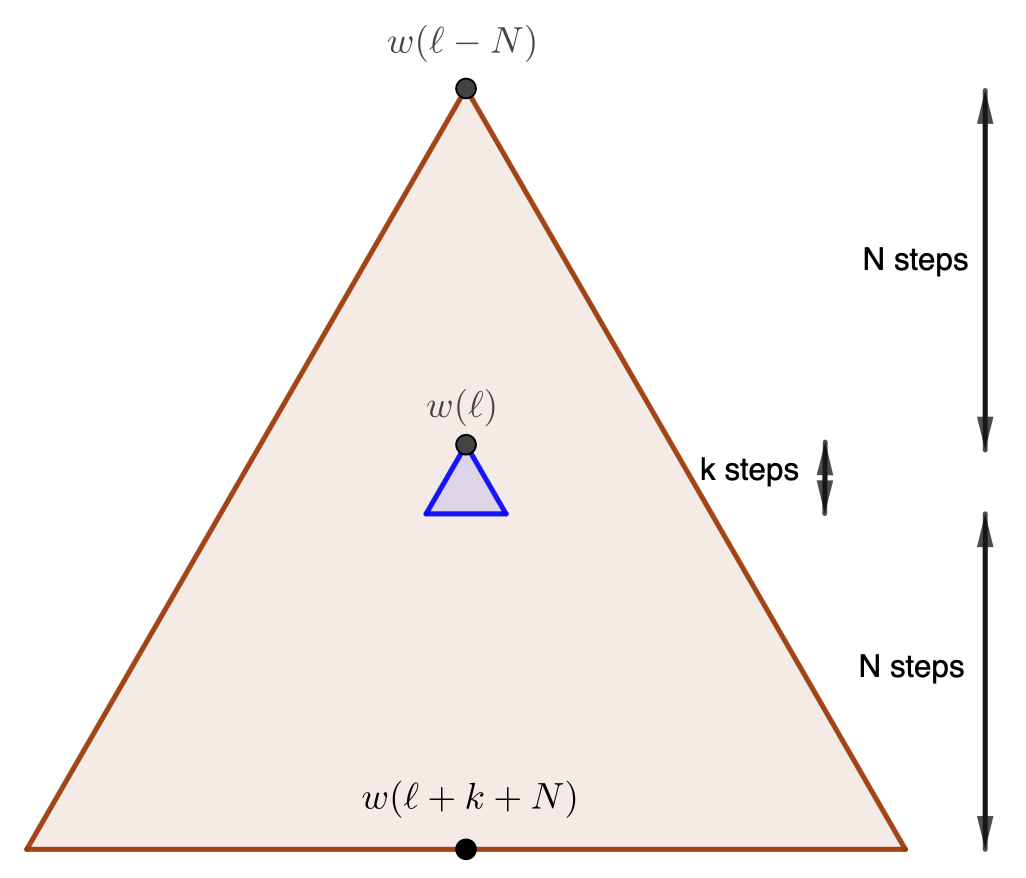
Figure 4. The big triangle represents all words in $\mathcal{A}_{n}^{*}$ that start with $w(\ell-N)$ and have at most $\ell+k+N$ letters. Words of the same the height have the same number of letters. The part of this set where $\eta$ takes the value 2 is colored by red, and the part of the set where $\eta$ takes the value 1 is colored by blue.

To simplify our notation, for a word $w\in\mathcal{A}_{n}^{\mathbb{N}}$, a function $\eta\in\mathscr{C}_{n}$, and two integers $N\geq 1,k\geq 0$, we say $(\eta,w,N,k)$ satisfies (R1), (R2) if there exists $\ell\in\mathbb{N}$ for which (R1) and (R2) hold. For a word $w\in\mathcal{A}^{\mathbb{N}}_{n}$ and a function $\eta\in\mathscr{C}_{n}$, we say that $(\eta,w)$ satisfies (R1) and (R2) if for every pair of integers $N\geq 1,k\geq 0$ , we have that $(\eta,w,N,k)$ satisfies (R1) and (R2). Thus, a choice function $\eta$ is random if for $\nu_{n}$-a.e. $w\in\mathcal{A}^{\mathbb{N}}_{n}$, $(\eta,w)$ satisfies (R1) and (R2).

The goal of this section is to show that random choice functions exist. In fact, we prove the following stronger statement.

Proposition 7.1.

For every even integer $n\geq 4$, $\mu_{n}$-a.e. $\eta\in\mathscr{C}_{n}$ is random.

Since $\pi_{\eta}\#\nu_{n}$ and $\mathcal{H}^{\alpha_{n}}\hbox{ {\vrule height=6.25963pt}{\leaders\hrule\hskip 5.69046pt} }K^{\eta}$ have the same null sets in $K^{\eta}$ for every $\eta\in\mathscr{C}_{n}$, Proposition 7.1 yields immediately the following corollary.

Corollary 7.2.

For every even integer $n\geq 4$, there exists $\eta\in\mathscr{C}_{n}$ such that $\mathcal{H}^{\alpha_{n}}$-almost every point $x\in K^{\eta}$ has $\pi_{\eta}^{-1}(\{x\})=\{w\}$ and $(\eta,w)$ satisfies (R1) and (R2).

Before proving Proposition 7.1, we establish some notation. For $w\in\mathcal{A}_{n}^{\mathbb{N}}$ define

$$D^{w}:=\{\eta\in\mathscr{C}_{n}:(\eta,w)\text{ satisfies (R1) and (R2)}\}$$

and for $\eta\in\mathscr{C}_{n}$ define

$$C_{\eta}:=\{w\in\mathcal{A}_{n}^{\mathbb{N}}:(\eta,w)\text{ satisfies (R1) and (R2)}\}.$$

Define also

$$\Delta_{n}:=\{(\eta,w)\in\mathscr{C}_{n}\times\mathcal{A}_{n}^{\mathbb{N}}:w\in C_{\eta}\}=\{(\eta,w)\in\mathscr{C}_{n}\times\mathcal{A}_{n}^{\mathbb{N}}:\eta\in D^{w}\}.$$

Proof of Proposition 7.1.

Using the notation above, we claim that $\mu_{n}(D^{w})=1$ for $\nu_{n}$-almost every word $w\in\mathcal{A}_{n}^{\mathbb{N}}$. Assuming the claim, by Fubini’s theorem we obtain

$$\int_{\mathscr{C}_{n}}\nu_{n}(C_{\eta})d\mu_{n}(\eta)=(\mu_{n}\times\nu_{n})(\Delta_{n})=\int_{\mathcal{A}_{n}^{\mathbb{N}}}\mu_{n}(D^{w})d\nu_{n}(w)=1.$$

Therefore, $\nu_{n}(C_{\eta})=1$ for $\mu_{n}$-a.e. $\eta\in\mathscr{C}_{n}$ which implies that $\mu_{n}$-a.e. $\eta\in\mathscr{C}_{n}$ is random.

For the proof of the claim, recall that

$$\nu_{n}(\{i_{1}i_{2}\cdots\in\mathcal{A}_{n}^{\mathbb{N}}:i_{j}>4n-4\text{ infinitely often}\})=1,$$

so it suffices to show that the claim holds for every word $w$ in the above set.

Fix $w=i_{1}i_{2}\cdots\in\mathcal{A}_{n}^{\mathbb{N}}$ such that $i_{j}>4n-4$ infinitely often. Fix also integers $N\geq 1$ and $k\geq 0$. We construct a sequence $(M_{m})_{m\in\mathbb{N}}\subset\mathbb{N}$ in an inductive fashion. Let $M_{1}\in\mathbb{N}$ be such that $i_{M_{1}+1}>4n-4$. Assuming that we have defined $M_{m}$ for some $m\in\mathbb{N}$, let $M_{m+1}\in\mathbb{N}$ such that $M_{m+1}>M_{m}+2N+k+1$ and $i_{M_{m+1}+1}>4n-4$.

For each $m\in\mathbb{N}$ let $E_{m,w}$ be the set of all choice functions $\eta\in\mathscr{C}_{n}$ such that $(\eta,w,N,k)$ satisfies (R1) and (R2) with $\ell=M_{m}+N$. Since $i_{M_{m}+1}>4n-4$ for each $m\in\mathbb{N}$, (R2) is satisfied for $\ell=M_{m}+N$. For each $m\in\mathbb{N}$, let

$$B_{m}=\bigcup_{j=0}^{2N+k-1}\mathcal{A}_{n,w(M_{m})}^{M_{m}+j},$$

that is, the set of of all finite words $u$ starting with $w(M_{m})$ and having length at most $M_{m}+2N+k-1$. Define also for each $m\in\mathbb{N}$ the function $\xi_{m}:B_{m}\to\{1,2\}$ via

$$\xi_{m}\left|\bigcup_{j=0}^{k-1}\mathcal{A}_{n,w(M_{m})}^{M_{m}+j}=1\right.\qquad\text{and}\qquad\xi_{m}\left|B_{m}\setminus\bigcup_{j=0}^{k-1}\mathcal{A}_{n,w(M_{m})}^{M_{m}+j}=2.\right.$$

Then, $E_{m,w}=\{\eta\in\mathscr{C}_{n}:\eta|_{B_{m}}=\xi_{m}\}$ and $|B_{m}|=\tfrac{(5n-6)^{2N+k}-1}{5n-7}$ for every $m\in\mathbb{N}$. By uniformity of the measure $\mu_{n}$, we have that for every $m\in\mathbb{N}$, $\mu_{n}(E_{m,w})=2^{-|B_{m}|}$, in particular each set $E_{m,w}$ has the same measure independent of $m$, and that measure is positive.

Next we claim that the sets $(E_{m,w})_{m\in\mathbb{N}}$ are independent. To see this, let $\{E_{m_{1},w},E_{m_{2},w},\cdots,E_{m_{j},w}\}$ be a finite collection of the sets $(E_{m,w})_{m\in\mathbb{N}}$, and note that

$$\bigcap\limits_{i=1}^{j}E_{m_{i},w}=\{\eta\in\mathscr{C}_{n}:\eta|_{B_{m_{i}}}=\xi_{m_{i}}\text{ for }i\in\{1,2,\cdots,j\}\}.$$

Since the sets $\{B_{m}\}_{m\in\mathbb{N}}$ are pairwise disjoint as $M_{m+1}-M_{m}>2N+k+1$, we have that $|\bigcup_{i=1}^{j}B_{m_{i}}|=\sum_{i=1}^{j}|B_{m_{i}}|$ and $\mu_{n}(\bigcap_{i=1}^{j}E_{m_{i},w})=2^{-|\bigcup_{i=1}^{j}B_{m_{i}}|}$. Thus,

$$\mu_{n}(\bigcap_{i=1}^{j}E_{m_{i},w})=\prod_{i=1}^{j}\mu_{n}(E_{m_{i},w}).$$

so the sets $(E_{m,w})_{m\in\mathbb{N}}$ are independent.

Furthermore, each set $E_{m,w}$ has the same positive measure, so

$$\sum_{m=1}^{\infty}\mu_{n}(E_{m,w})=\infty.$$

Thus, by the second Borel-Cantelli Lemma,

$$\mu_{n}(\bigcap_{j=1}^{\infty}\bigcup_{m=j}^{\infty}E_{m,w})=1,$$

or equivalently, for $\mu_{n}$-almost every choice function $\eta\in\mathscr{C}_{n}$, $(\eta,w,N,k)$ satisfies (R1) and (R2) infinitely often. In particular, for every pair of integers $N\geq 1,k\geq 0$ we have that for $\mu_{n}$-almost every $\eta\in\mathscr{C}_{n}$, $(\eta,w,N,k)$ satisfies (R1) and (R2). Since there are countably many choices of $N$ and $k$, we have immediately that $\mu_{n}(D^{w})=1$ for $\nu_{n}$-almost every word $w\in\mathcal{A}^{\mathbb{N}}_{n}$. ∎

8. Tangents of carpets $K^{\eta}$ at typical points

Fix for the rest of this section an even integer $n\geq 4$ and denote by ${\bf 0}$ the origin $(0,0)$. Recall the definitions of choice functions $\eta\in\mathscr{C}_{n}$ and carpets $K^{\eta}$ from Section 4, the number $\alpha_{n}=\frac{\log(5n-6)}{\log(n)}$ from Section 5, and the definition of random choice functions from Section 7.

In this section we prove the following result about weak tangents of carpets $K^{\eta}$ at typical points when $\eta$ is random.

Proposition 8.1.

If $\eta\in\mathscr{C}_{n}$ is a random choice function, then for $\mathcal{H}^{\alpha_{n}}$-a.e. $x\in K^{\eta}$ there exist $T_{n,0},T_{n,1},T_{n,2},\dots\in\operatorname{Tan}(K^{\eta},x)$ such that $T_{n,k}$ has exactly $\frac{1}{5n-7}((5n-6)^{k}-1)$ many cut points.

In §8.1 we study the local cut-points of a certain class of “almost self-similar” carpets and in §8.2, we relate the tangents of $K^{\eta}$ with these carpets.

8.1. Local cut-points in a class of carpets

Define, for an integer $k\geq 0$, the set

(8.1) $$K^{n,k}:=\bigcup\limits_{w\in\mathcal{A}_{n}^{k}}\psi_{n,w}^{1}\left(\bigcap\limits_{m=1}^{\infty}\bigcup\limits_{v\in\mathcal{A}_{n}^{m}}\psi_{n,v}^{2}([0,1]^{2})\right)$$

where maps $\psi_{n,v}^{i}$ and $\phi_{v}^{\eta}$ for $v\in\mathcal{A}_{n}^{*}$ and $i\in\{1,2\}$ are as in Section 4.

Roughly speaking, $K^{n,k}$ is obtained by first iterating $k$ times the maps from the system $\mathcal{F}_{n}^{1}$, and then applying these iterates to the self-similar attractor of the IFS of similarities $\mathcal{F}_{n}^{2}$ (recall the systems $\mathcal{F}_{n}^{1},\mathcal{F}_{n}^{2}$ from Section 4).

The next lemma is the main result of this subsection.

Lemma 8.2.

For each integer $k\geq 0$, $K^{n,k}$ has exactly $\frac{1}{5n-7}((5n-6)^{k}-1)$ many local cut-points.

The proof of Lemma 8.2 is by induction on $k$. The base case $k=0$ is given in Lemma 8.6. In the proof, we make use of the following definition.

Let $\{f_{j}(x)=Lx+b_{j}\}_{j=1}^{l}$ be similarities on $\mathbb{R}^{2}$ where $L>0$ and $l\geq 2$ such that

1. if $i,j\in\{1,\dots,l\}$ are distinct, then, $f_{i}((0,1)^{2})\cap f_{j}((0,1)^{2})=\emptyset$, and

2. $\bigcap_{i=1}^{l}f_{i}([0,1]^{2})\neq\emptyset$.

We say that $f_{1},\dots,f_{l}$ meet at edges of $[0,1]^{2}$ if for every $i\in\{1,\dots,l\}$, there exists $j\in\{1,\dots,l\}\setminus\{i\}$ so that $f_{i}([0,1]^{2})\cap f_{j}([0,1]^{2})$ is an edge of $f_{i}([0,1]^{2})$. Note that necessarily $l\in\{2,3,4\}$.

Remark 8.3.

Recall from the proof of Lemma 4.3 that for any $k\in\mathbb{N}$,

$$\bigcup_{j\in\mathcal{A}_{n}}\psi_{n,j}^{2}(\partial[0,1]^{2})\subset K^{n,0}\subset\bigcup_{j\in\mathcal{A}_{n}}\psi_{n,j}^{2}([0,1]^{2})$$

$$\bigcup_{j\in\mathcal{A}_{n}}\psi_{n,j}^{1}(\partial[0,1]^{2})\subset K^{n,k}\subset\bigcup_{j\in\mathcal{A}_{n}}\psi_{n,j}^{1}([0,1]^{2}).$$

Note also that if there exist distinct $i,j\in\mathcal{A}_{n}$ and $x\in[0,1]^{2}$ with $x\in\psi_{n,j}^{2}([0,1]^{2})\cap\psi_{n,i}^{2}([0,1]^{2})$, then the maps in $\{\psi_{n,l}^{2}:x\in\psi_{n,l}^{2}([0,1]^{2}),l\in\mathcal{A}_{n}\}$ meet at edges of $[0,1]^{2}$. Note further that if there exist distinct $i,j\in\mathcal{A}_{n}$ and $x\in[0,1]^{2}$ with $x\in\psi_{n,j}^{2}([0,1]^{2})\cap\psi_{n,i}^{2}([0,1]^{2})$, then either $x=(1/2,2/n)$ or the functions in the set $\{\psi_{n,l}^{1}:x\in\psi_{n,l}^{1}([0,1]^{2}),l\in\mathcal{A}_{n}\}$ meet at edges of $[0,1]^{2}$. See for example Figure 2 for the case $n=6$.

Lemma 8.4.

Let $\eta\in\mathscr{C}_{n}$, let $m\in\mathbb{N}$, let $u,v,w\in\mathcal{A}_{n}^{m}$ be distinct, and let $x\in\phi_{u}^{\eta}([0,1]^{2})\cap\phi_{v}^{\eta}([0,1]^{2})\cap\phi_{w}^{\eta}([0,1]^{2})$. Then the maps $\{\phi_{\beta}^{\eta}:x\in\phi_{\beta}^{\eta}([0,1]^{2}),\beta\in\mathcal{A}_{n}^{m}\}$ meet at edges of $[0,1]^{2}$.

Proof.

Recall that for all $\beta\in\mathcal{A}_{n}^{m}$, $\phi_{\beta}^{\eta}(x)=n^{-m}y+\phi_{\beta}^{\eta}({\bf 0})$ with $\phi_{\beta}^{\eta}({\bf 0})\in\{0,\frac{1}{n^{m}},\dots,\frac{n^{m}-1}{n^{m}}\}^{2}$.

Let $E=\{\beta\in\mathcal{A}_{n}^{m}:x\in\phi_{\beta}^{\eta}([0,1]^{2})\}$ which, by assumption, contains at least three words. Clearly the intersection $\bigcap_{\beta\in E}\phi_{\beta}^{\eta}([0,1]^{2})$ is nonempty as it contains $x$.

Suppose that $a,b\in E$ are distinct words so that $\phi_{a}^{\eta},\phi_{b}^{\eta}$ do not meet at edges of $[0,1]^{2}$. Then $\phi_{a}^{\eta}({\bf 0})-\phi_{b}^{\eta}({\bf 0})\in\{-n^{-m},n^{-m}\}^{2}$. Since $\operatorname{card}(E)\geq 3$, there exists $c\in E\setminus\{a,b\}$ with

$$\phi_{a}^{\eta}({\bf 0})-\phi_{c}^{\eta}({\bf 0})\in\{-n^{-m},0,n^{-m}\}^{2},\qquad\phi_{b}^{\eta}({\bf 0})-\phi_{c}^{\eta}({\bf 0})\in\{-n^{-m},0,n^{-m}\}^{2}.$$

If, for example, $\phi_{a}^{\eta}({\bf 0})-\phi_{c}^{\eta}({\bf 0})\in\{-n^{-m},n^{-m}\}^{2}$, then

$$\phi_{c}^{\eta}({\bf 0})-\phi_{b}^{\eta}({\bf 0})=(\phi_{c}^{\eta}({\bf 0})-\phi_{a}^{\eta}({\bf 0}))+(\phi_{a}^{\eta}({\bf 0})-\phi_{b}^{\eta}({\bf 0}))\in\{-2n^{-m},0,2n^{-m}\}^{2}\cap\{-n^{-m},0,n^{-m}\}^{2}.$$

But then $\phi_{c}^{\eta}({\bf 0})=\phi_{b}^{\eta}({\bf 0})$, and this is a contradiction. Hence, $\phi_{a}^{\eta}({\bf 0})-\phi_{c}^{\eta}({\bf 0})\notin\{-n^{-m},n^{-m}\}^{2}$, and by a simple calculation we get $\phi_{a}^{\eta}([0,1]^{2})\cap\phi_{c}^{\eta}([0,1]^{2})$ is equal to an edge of $\phi_{a}^{\eta}([0,1]^{2})$ containing $x$, and similarly for $\phi_{b}^{\eta}([0,1]^{2})\cap\phi_{c}^{\eta}([0,1]^{2})$. From this we may conclude that the maps in $\{\phi_{\beta}^{\eta}:\beta\in E\}$ meet at edges of $[0,1]^{2}$. ∎

Lemma 8.5.

Let $m\in\mathbb{N}$, let $u,v\in\mathcal{A}_{n}^{m}$ be distinct, and let $x\in K^{n,0}$ with $a\in\psi_{n,u}^{2}(K^{n,0})\cap\psi_{n,v}^{2}(K^{n,0})$. Then the maps in $\{\psi_{n,w}^{2}:x\in\psi_{n,w}^{2}(K^{n,0}),w\in\mathcal{A}_{n}^{m}\}$ meet at edges of $[0,1]^{2}$.

Proof.

The proof is by induction on $m$. The base case $m=1$ holds by Remark 8.3.

Assume now that the claim holds for some $m\in\mathbb{N}$. Let $x\in K^{n,0}$ and $u,v\in\mathcal{A}_{n}^{m+1}$ distinct so that $x\in\psi_{n,u}^{2}(K^{n,0})\cap\psi_{n,v}^{2}(K^{n,0})$. By Lemma 8.4, we may assume that $\{w\in\mathcal{A}_{n}^{m+1}:x\in\psi_{n,w}^{2}(K^{n,0})\}=\{u,v\}$. We prove that $\psi_{n,u}^{2}(K^{n,0})\cap\psi_{n,w}^{2}(K^{n,0})$ is an edge of $\psi_{n,u}^{2}([0,1]^{2})$.

Let $u=a_{1}\dots a_{m+1},v=b_{1}\dots b_{m+1}$. If $a_{1}=b_{1}$, then applying $(\psi_{n,a_{1}}^{2})^{-1}$ returns us to the claim at $m$, so by the inductive hypothesis we may assume that $a_{1}\neq b_{1}$. Next, if $x$ is not a vertex of $\psi_{n,u}^{2}([0,1]^{2})$, then by Lemma 10.2 the claim holds, so we may further assume that $x$ is a vertex of $\psi_{n,u}^{2}([0,1]^{2})$ and of $\psi_{n,v}^{2}([0,1]^{2})$. If there exists a word $w\in\mathcal{A}_{n}^{m}\setminus\{u(m),v(m)\}$ so that $x\in\psi_{n,w}^{2}(K^{n,0})$, then there exists a $j\in\mathcal{A}_{n}$ with $x\in\psi_{n,u}^{2}(K^{n,0})\cap\psi_{n,v}^{2}(K^{n,0})\cap\psi_{n,wj}^{2}(K^{n,0})$, and this is a contradiction.

Therefore, we may further assume that $\{w\in\mathcal{A}_{n}^{m}:x\in\psi_{n,w}^{2}(K^{n,0})\}=\{v(m),u(m)\}$. Then by the inductive hypothesis, $\psi_{n,u(m)}^{2}(K^{n,0})\cap\psi_{n,v(m)}^{2}(K^{n,0})$ is an edge of $\psi_{n,u(m)}^{2}([0,1]^{2})$. The remainder of the proof is a case study on which edge of $\psi_{n,u(m)}^{2}([0,1]^{2})$ this intersection is equal to, but these cases are all essentially identical so we show only one of them and leave the remaining three to the reader. Assume that

$$\psi_{n,u(m)}^{2}(K^{n,0})\cap\psi_{n,v(m)}^{2}(K^{n,0})=\psi_{n,u(m)}^{2}([0,1]\times\{0\}),$$

and as the maps $\psi_{n,u(m)}^{2}$ and $\psi_{n,v(m)}^{2}$ are both rotation-free and reflection-free similarity maps with Lipschitz norms $n^{-m}$, by Remark 2.8 this intersection must also be equal to the edge $\psi_{n,v(m)}^{2}([0,1]\times\{1\})$. Then

$$\psi_{n,u(m)}^{2}({\bf 0})-\psi_{n,v(m)}^{2}({\bf 0})=(0,n^{-m}),\quad\psi_{n,a_{m+1}}^{2}({\bf 0})=(\tfrac{k}{n},0),\quad\psi_{n,b_{m+1}}^{2}({\bf 0})=(\tfrac{k\pm 1}{n},1)$$

with $k,k\pm 1\in\{0,1,\dots,n-1\}$. Then there is some $j\in\mathcal{A}_{n}$ so that $\psi_{n,j}^{2}({\bf 0})=(\frac{k}{n},1)$, thus by a straightforward calculation we obtain $x\in\psi_{n,v(m)j}^{2}(K^{n,0})$. As $a_{1}\neq b_{1}$ and necessarily $j\neq b_{m+1}$, $v(m)j\in\mathcal{A}_{n}^{m+1}\setminus\{v,u\}$, and this contradicts our assumption that $\{w\in\mathcal{A}_{n}^{m+1}:x\in\psi_{n,w}^{2}(K^{n,0})\}=\{u,v\}$, concluding the proof. ∎

Lemma 8.6.

The set $K^{n,0}$ does not contain local cut-points.

Proof.

It suffices to show that $K^{n,0}$ contains no cut-points. Assuming the latter to be true, the proof of the lemma follows from [DLR⁺23, Theorem 1.6], as Lemma 8.4 and Lemma 8.5 alongside the fact that $K^{n,0}$ is a self-similar set with no cut-points are sufficient to imply the hypotheses of this theorem.

To prove that $K^{n,0}$ contains no cut-points, fix $y\in K^{n,0}$ and distinct $p,q\in K^{n,0}\setminus\{y\}$. Let $m\in\mathbb{N}$ so that there exist distinct $u,v,w\in\mathcal{A}_{n}^{m}$ for which $\psi_{n,u}^{2}(K^{n,0})$, $\psi_{n,v}^{2}(K^{n,0})$, and $\psi_{n,w}^{2}(K^{n,0})$ are pairwise disjoint with $p\in\psi_{n,v}^{2}(K^{n,0})$, $q\in\psi_{n,u}^{2}(K^{n,0})$, and $y\in\psi_{n,w}^{2}(K^{n,0})$. Then by Lemma 8.5 and by [BV21, Lemma 3.1], there exist distinct $u_{1},\dots,u_{k}\in\mathcal{A}_{n}^{m}$ so that $p\in\psi_{n,u_{1}}^{2}(K^{n,0})$, $q\in\psi_{n,u_{k}}^{2}(K^{n,0})$, and for every $j\in\{1,\dots,k-1\}$, $\psi_{n,u_{j}}^{2}(K^{n,0})\cap\psi_{n,u_{j+1}}^{2}(K^{n,0})$ contains at least two points. Now let $z_{0},\dots,z_{k}\in K^{n,0}$ be distinct points so that $z_{0}=p$, $z_{k}=q$, and $z_{j}\in(\psi_{n,u_{j}}^{2}(K^{n,0})\cap\psi_{n,u_{j+1}}^{2}(K^{n,0}))\setminus\{y\}$ for every $j\in\{1,\dots,k-1\}$ . Then since $\partial[0,1]^{2}\subset K^{n,0}$ by the proof of Lemma 4.3, for every $j\in\{1,\dots,k-2\}$ there is a continuous function $\gamma_{j}:[0,1]\to\psi_{n,u_{j+1}}^{2}(\partial[0,1]^{2})\setminus\{y\}$ so that $\gamma_{j}(0)=z_{j}$, $\gamma_{j}(1)=z_{j+1}$ and necessarily $\gamma_{j}([0,1])\subset K^{n,0}\setminus\{y\}$. By [BV21, Proposition 3.2], there exist continuous $\gamma_{0}:[0,1]\to\psi_{n,u_{1}}^{2}(K^{n,0})$ with $\gamma_{0}(0)=p$, $\gamma_{0}(1)=z_{1}$ and continuous $\gamma_{k-1}:[0,1]\to\psi_{n,u_{k}}^{2}(K^{n,0})$ with $\gamma_{k-1}(0)=z_{k-1}$, $\gamma_{k-1}(1)=q$. Concatenating these curves yields a path inside of $K^{n,0}$ connecting $p$ to $q$ and avoiding $y$, so $y$ cannot be a cut-point for $K^{n,0}$. ∎

As a straightforward consequence, we obtain the following corollary.

Corollary 8.7.

If $f_{1},\dots,f_{j}:\mathbb{R}^{2}\to\mathbb{R}^{2}$ with $j\in\{2,3,4\}$ is a collection of rotation-free and reflection-free similarity maps with a common Lipschitz norm which meet at edges of $[0,1]^{2}$, then $\bigcup_{i=1}^{j}f_{i}(K^{n,0})$ does not contain local cut-points.

Proof.

We leave most of this proof as an exercise to the reader. A proof follows from the observation that, up to re-scaling and translating, there are only $7$ ways for such a collection of maps to meet at edges of $[0,1]^{2}$, and all of these arrangements are present in $\{\psi_{n,j}^{2}:j\in\mathcal{A}_{n}\}$. ∎

We are now finally ready to prove Lemma 8.2.

Proof of Lemma 8.2.

Denote by $N_{k}$ the number of local cut-points in $K^{n,k}$. By Lemma 8.6 we have $N_{0}=0$. It remains to show that $N_{k}=(5n-6)N_{k-1}+1$ for every $k\in\mathbb{N}$.

By definition of sets $K^{n,k}$,

$$K^{n,k} =\bigcup\limits_{v\in\mathcal{A}_{n}^{k}}\psi_{n,v}^{1}\left(\bigcap\limits_{m\in\mathbb{N}}\bigcup\limits_{w\in\mathcal{A}_{n}^{m}}\psi_{n,w}^{2}([0,1]^{2})\right)$$

$$=\bigcup\limits_{j\in\mathcal{A}_{n}}\psi_{n,j}^{1}\left(\bigcup\limits_{v\in\mathcal{A}_{n}^{k-1}}\psi_{n,v}^{1}\left(\bigcap\limits_{m\in\mathbb{N}}\bigcup\limits_{w\in\mathcal{A}_{n}^{m}}\psi_{n,w}^{2}([0,1]^{2})\right)\right)$$

$$=\bigcup\limits_{j\in\mathcal{A}_{n}}\psi_{n,j}^{1}(K^{n,k-1}).$$

By Lemma 4.2, each $\psi_{n,j}^{1}(K^{n,k-1}\cap(0,1)^{2})$ contributes $N_{k-1}$ many local cut-points, and there is one additional local cut-point at $(1/2,2/n)$. Then by the last part of Remark 8.3, every point of $K^{n,k}\setminus(\bigcup_{j\in\mathcal{A}_{n}}\psi_{n,j}^{1}(K^{n,k-1}\cap(0,1)^{2})$ other than $(1/2,2/n)$ is either contained in exactly one image $\psi_{n,v}^{1}(K^{n,0})$ for some $v\in\mathcal{A}_{n}^{k}$ or in an intersection of at least two such images of maps which meet at edges of $[0,1]^{2}$, so there are no other local cut-points of $K^{n,k}$ by Corollary 8.7. Therefore, $N_{k}=(5n-6)N_{k-1}+1$. ∎

8.2. Proof of Proposition 8.1

Fix for the rest of this section an integer $k\geq 0$, a random choice function $\eta\in\mathscr{C}_{n}$, and an injective word (see the paragraph before Lemma 5.3 for the definition of injective words)

$$w=i_{1}i_{2}\dots\in\mathcal{A}^{\mathbb{N}}_{n}$$

such that $(\eta,w)$ satisfy (R1) and (R2) from the definition of a random choice function. Set $x=\pi_{\eta}(w)$. Given $N\in\mathbb{N}$, let $\ell_{N}\in\mathbb{N}$ be the integer given in properties (R1) and (R2). For $N\in\mathbb{N}$, define

$$X_{N} :=n^{\ell_{N}}(K^{\eta}-x),$$

$$y_{N} :=(\phi^{\eta}_{w(\ell_{N})})^{-1}\circ\phi^{\eta}_{w(\ell_{N}+N+k-1)}({\bf 0}),$$

$$x_{N} :=n^{\ell_{N}}(x-\phi^{\eta}_{w(\ell_{N})}({\bf 0})).$$

Intuitively, $x_{N}$ are the bottom-left corners of the blow-ups of pieces of $K^{\eta}$ that contain $x$, while the points $(y_{N})_{N\in\mathbb{N}}$ form a sequence of points in $[0,1]^{2}$ which approximate the points $x_{N}$. Additionally, the sets $X_{N}$ are a sequence of blow-ups of $K^{\eta}$ centered at the point $x$ which we use to find the desired weak tangents in $\operatorname{Tan}(K^{\eta},x)$.

By (R2), $i_{\ell_{N}-N+1}>(4n-4)$, so $\psi^{\eta(w(\ell_{N}-N))}_{n,i_{\ell_{N}-N+1}}([0,1]^{2})$ does not intersect $\partial[0,1]^{2}$, thus for every $N\geq 3$ we get

(8.2) $$\operatorname{dist}\left(K^{\eta}_{w(\ell_{N})},K^{\eta}\setminus K^{\eta}_{w(\ell_{N}-N)}\right)\geq n^{-\ell_{N}-1+N}.$$

The general strategy of the proof of Proposition 8.1 is to first establish estimates for the Hausdorff distance between $X_{N}$ and translates of $K^{n,k}$ in a region near $[0,1]^{2}$, then establish estimates for the Hausdorff distance between the rest of $X_{N}$ and some blown-up and translated image of $K^{n,0}$ out to some large ball containing the origin. Then, exploiting the triangle inequality for excess (as in Remark 2.2), we show that some subsequence of $X_{N}$ converges to a weak tangent set for which all local cut-points (see §2.5) lie inside a unit square near the origin, for which outside of this square the weak tangent “looks like” a weak tangent of $K^{n,0}$, and for which inside this unit square the weak tangent has exactly $\frac{1}{5n-7}((5n-6)^{k}-1)$ many local cut-points.

Lemma 8.8.

For each $N\in\mathbb{N}$, $|y_{N}-x_{N}|\leq n^{-N-k+3}$.

Proof.

Since $x=\pi_{\eta}(w)$, the point $x_{N}$ is in the set

$$n^{\ell_{N}}(\phi_{w(\ell_{N}+N+k-1)}^{\eta}([0,1]^{2}) -\phi_{w(\ell_{N})}^{\eta}({\bf 0}))$$

$$=n^{\ell_{N}}\left(\phi^{\eta}_{w(\ell_{N})}\circ(\phi_{w(\ell_{N})}^{\eta})^{-1}\circ\phi^{\eta}_{w(\ell_{N}+N+k-1)}([0,1]^{2})-\phi^{\eta}_{w(\ell_{N})}({\bf 0})\right).$$

Now by Remark 2.8, the latter set is equal to $(\phi_{w(\ell_{N})}^{\eta})^{-1}\circ\phi^{\eta}_{w(\ell_{N}+N+k-1)}([0,1]^{2})$, which has diameter no more than $n^{-N-k+2}\sqrt{2}$ and contains $y_{N}$, so $|y_{N}-x_{N}|\leq n^{-N-k+3}$. ∎

In the following lemma, we show that the parts of the sets $X_{N}$ inside of some unit square containing the origin become close to translates of $K^{n,k}$ in terms of Hausdorff distance.

Lemma 8.9.

For each $N\in\mathbb{N}$, the Hausdorff distance

$$\operatorname{dist_{H}}(n^{\ell_{N}}(K^{\eta}_{w(\ell_{N})}-x),K^{n,k}-y_{N})\leq n^{-N-k+4}.$$

Proof.

Recall that if $A,B\subset\mathbb{R}^{M}$ are compact sets, then Hausdorff distance is given by

$$\operatorname{dist_{H}}(A,B):=\max\left\{\sup_{x\in A}\inf_{y\in B}|x-y|,\sup_{y\in B}\inf_{x\in A}|y-x|\right\},$$

and recall from §2.4 that excess is given by $\operatorname{excess}(A,B):=\sup_{x\in A}\inf_{y\in B}|x-y|$. Thus to prove the lemma, it suffices to show

$$\operatorname{excess}(n^{\ell_{N}}(K^{\eta}_{w(\ell_{N})}-x),K^{n,k}-y_{N})\leq n^{-N-k+4},$$

$$\operatorname{excess}(K^{n,k}-y_{N},n^{\ell_{N}}(K^{\eta}_{w(\ell_{N})}-x))\leq n^{-N-k+4}.$$

For the first inequality, by Lemma 8.8 and by the triangle inequality for excess as in Remark 2.2, it is enough to show that

$$\operatorname{excess}(n^{\ell_{N}}(K^{\eta}_{w(\ell_{N})}-x),K^{n,k}-x_{N})\leq n^{-N-k+3}.$$

Note that since excess is translation invariant (see Remark 2.2), this excess is equal to

$$\operatorname{excess}(n^{\ell_{N}}(K^{\eta}_{w(\ell_{N})}-\phi^{\eta}_{w(\ell_{N})}({\bf 0})),K^{n,k}),$$

which is at most $n^{-N-k+2}\sqrt{2}$ by (R1) and by definition of $K^{n,k}$. Via a similar argument, we obtain the other inequality

$$\operatorname{excess}(K^{n,k}-y_{N},n^{\ell_{N}}(K^{\eta}_{w(\ell_{N})}-x))\leq n^{-N-k+4}.\qed$$

Now define

$$F_{N} :=n^{\ell_{N}}(K^{n,0}-\phi_{w(\ell_{N})}^{\eta}({\bf 0}))-y_{N},$$

$$Y_{N} :=(F_{N}\setminus([0,1]^{2}-y_{N}))\cup(K^{n,k}-y_{N}).$$

The sets $F_{N}$ are simply blown-up shifts of the self-similar set $K^{n,0}$. The sets $Y_{N}$ are constructed by removing the copy of $K^{n,0}$ in $F_{N}$ which contains the origin, then replacing it by a shift of $K^{n,k}$. Before continuing, note that for $k=0$, $F_{N}=Y_{N}$.

Lemma 8.10.

For every $r>0$,

$$\lim\limits_{N\to\infty}\operatorname{excess}(Y_{N}\cap\overline{B}({\bf 0},r),X_{N})=0\quad\text{and}\quad\lim\limits_{N\to\infty}\operatorname{excess}(X_{N}\cap\overline{B}({\bf 0},r),Y_{N})=0.$$

Proof.

Fix $r>0$. By (8.2) there exists $N_{0}\in\mathbb{N}$ such that for every integer $N\geq N_{0}$,

$$\operatorname{dist}(K^{\eta}_{w(\ell_{N})},K^{\eta}\setminus K^{\eta}_{w(\ell_{N}-N)})\geq n^{-\ell_{N}}2r.$$

By (R2), $\operatorname{dist}(\partial[0,1]^{2},(\phi_{w(\ell_{N}-N)}^{\eta})^{-1}\circ\phi_{w(\ell_{N})}^{\eta}({\bf 0}))\geq n^{-1}$. Since $y_{N}\in[0,1]^{2}$,

$$\overline{B}({\bf 0},r)\subset n^{N}([0,1]^{2}-(\phi_{w(\ell_{N}-N)}^{\eta})^{-1}\circ\phi_{w(\ell_{N})}^{\eta}({\bf 0}))-y_{N}.$$

Fix $y\in Y_{N}\cap\overline{B}({\bf 0},r)$. If $y\in[0,1]^{2}-y_{N}$, then by Lemma 8.9 there exists some $z\in X_{N}$ so that $|y-z|\leq n^{-N-k+4}$.

Assume now that $y\in Y_{N}\cap\overline{B}({\bf 0},r)\setminus([0,1]^{2}-y_{N})$. Let

$$Q=\bigcup_{v\in\mathcal{A}_{n}^{2N+k-1}}\psi_{n,v}^{2}([0,1]^{2})\quad\text{and}\quad P=\bigcup_{v\in\mathcal{A}_{n}^{2N+k-1}}\psi_{n,v}^{2}(\partial[0,1]^{2}).$$

By (R2) and since $\phi_{v}^{\eta}(\partial[0,1]^{2})\subset K^{\eta}$ for every finite word $v\in\mathcal{A}_{n}^{*}$ by the proof of Lemma 4.3, we have that

$$n^{\ell_{N}}((\phi_{w(\ell_{N}-N)}^{\eta}(P)-x)\setminus(\phi_{w(\ell_{N})}^{\eta}([0,1]^{2})-x))\subset X_{N}.$$

Since the maps $\psi_{n,j}^{i}$ are all similarities with Lipschitz norm $n^{-1}$, by Remark 2.8 we have

$$n^{\ell_{N}}(\phi_{w(\ell_{N}-N)}^{\eta}(P)-x) =n^{\ell_{N}}(\phi_{w(\ell_{N}-N)}^{\eta}(P)-\phi_{w(\ell_{N}-N)}^{\eta}\circ(\phi_{w(\ell_{N}-N)}^{\eta})^{-1}(x))$$

$$=n^{N}(P-(\phi_{w(\ell_{N}-N)}^{\eta})^{-1}(x)).$$

Similarly, we obtain $n^{\ell_{N}}(\phi_{w(\ell_{N})}^{\eta}([0,1]^{2})-x)=[0,1]^{2}-(\phi_{w(\ell_{N})}^{\eta})^{-1}(x)$ and $x_{N}=(\phi_{w(\ell_{N})}^{\eta})^{-1}(x)$. Furthermore, $(\phi_{w(\ell_{N}-N)}^{\eta})^{-1}(x)=(\phi_{w(\ell_{N}-N)}^{\eta})^{-1}\circ\phi_{w(\ell_{N})}^{\eta}(x_{N})$, and so

$$(n^{N}(P-(\phi_{w(\ell_{N}-N)}^{\eta})^{-1}\circ\phi_{w(\ell_{N})}^{\eta}({\bf 0}))-x_{N})\setminus([0,1]^{2}-x_{N})\subset X_{N}.$$

Since $y\in Y_{N}\cap\overline{B}({\bf 0},r)\setminus([0,1]^{2}-y_{N})$, by calculations similar to those above we obtain

$$y\in(n^{N}(Q-(\phi_{w(\ell_{N}-N)}^{\eta})^{-1}\circ\phi_{w(\ell_{N})}^{\eta}({\bf 0}))-y_{N})\setminus([0,1]^{2}-y_{N}).$$

Therefore, there exists $u\in\mathcal{A}_{n}^{2N+k-1}$ so that

$$y\in(n^{N}(\psi_{n,u}^{2}([0,1]^{2})-(\phi_{w(\ell_{N}-N)}^{\eta})^{-1}\circ\phi_{w(\ell_{N})}^{\eta}({\bf 0}))-y_{N})\setminus([0,1]^{2}-y_{N}),$$

which implies that there is a point

$$p\in(n^{N}(\psi_{n,u}^{2}(\partial[0,1]^{2})-(\phi_{w(\ell_{N}-N)}^{\eta})^{-1}\circ\phi_{w(\ell_{N})}^{\eta}({\bf 0}))-x_{N})\setminus([0,1]^{2}-x_{N}),$$

hence $p\in X_{N}$. Then by the triangle inequality and Lemma 8.8 we have

$$|p-y|\leq|x_{N}-y_{N}|+|(p+x_{N})-(y+y_{N})|\leq|x_{N}-y_{N}|+n^{-N-k+1}\sqrt{2}\leq n^{-N-k+4}$$

since $(p+x_{N}),(y+y_{N})\in n^{N}\psi_{n,u}^{2}([0,1]^{2})$, and the latter set has diameter $n^{-N-k+1}\sqrt{2}$.

The other limit can be proven in the same way, yielding the result.∎

In the following two lemmas, we prove that the sequence $(Y_{N})_{N\in\mathbb{N}}$ has a subsequence converging in the Attouch-Wets topology to a set with $\frac{1}{5n-7}((5n-6)^{k}-1)$ local cut-points and that the closeness of excesses from Lemma 8.10 implies that this set is also the Attouch-Wets limit of a subsequence of $(X_{N})_{N\in\mathbb{N}}$, thus it is a weak tangent of $K^{\eta}$ at $x$.

Lemma 8.11.

The sequence $(Y_{N})_{N\in\mathbb{N}}$ has a subsequence converging with respect to the Attouch-Wets topology to a set $L_{k}\in\mathfrak{C}(\mathbb{R}^{2};{\bf 0})$ that has exactly $\frac{1}{5n-7}((5n-6)^{k}-1)$ many local cut-points.

Proof.

Let $r>3$, and recall from the proof of Lemma 8.10 that there exists a minimal $N_{0,r}\in\mathbb{N}$ so that for every integer $N\geq N_{0,r}$,

$$(Y_{N}+y_{N})\cap\overline{B}({\bf 0},r)=\overline{B}({\bf 0},r)\cap(n^{N}(K^{n,0}-(\phi_{w(\ell_{N}-N)}^{\eta})^{-1}\circ\phi_{w(\ell_{N})}^{\eta}({\bf 0}))\setminus[0,1]^{2})\cup K^{n,k}.$$

Furthermore, $N_{0,r}$ is nondecreasing in $r$. By (R1), for each $N\in\mathbb{N}$ there exists a word $v_{N}\in\mathcal{A}_{n}^{N}$ so that $(\phi_{w(\ell_{N}-N)}^{\eta})^{-1}\circ\phi^{\eta}_{w(\ell_{N})}=\psi_{n,v_{N}}^{2}$. Then by the OSC and since these maps are affine, by Remark 2.8 we obtain

$$[0,1]^{2}\cap n^{N}(K^{n,0}-\psi_{n,v_{N}}^{2}({\bf 0}))=n^{N}(\psi_{n,v_{N}}^{2}(K^{n,0})-\psi_{n,v_{N}}^{2}({\bf 0}))=K^{n,0}.$$

Thus,

$$(Y_{N}+y_{N})\cap\overline{B}({\bf 0},r)=\overline{B}({\bf 0},r)\cap(n^{N}(((K^{n,0}\setminus\psi_{n,v_{N}}^{2}([0,1]^{2}))\cup(\psi_{n,v_{N}}^{2}(K^{n,k})))-\psi_{n,v_{N}}^{2}({\bf 0}))).$$

Since $\mathfrak{C}(\mathbb{R}^{2};{\bf 0})$ is sequentially compact in the Attouch-Wets topology, the sequence of sets $(Y_{N}+y_{N})_{N\in\mathbb{N}}$ has a subsequence $(Y_{N_{j}}+y_{N_{j}})_{j\in\mathbb{N}}$ converging to a limit $L$ in the Attouch-Wets topology and so that $(y_{N_{j}})_{j\in\mathbb{N}}$ converges to a point $y_{0}\in[0,1]^{2}$ as $j\to\infty$.

For $r>3$ and $j\in\mathbb{N}$, let

$$D_{r,j} :=\{(m_{1},m_{2})\in\mathbb{Z}^{2}\setminus\{{\bf 0}\}:[m_{1},m_{1}+1]\times[m_{2},m_{2}+1]\subset\overline{B}({\bf 0},r),$$

$$\text{ and there exists }v\in\mathcal{A}_{n}^{N_{j}}\text{ with }(m_{1},m_{2})=n^{N_{j}}(\psi_{n,v}^{2}({\bf 0})-\psi_{n,v_{N_{j}}}^{2}({\bf 0}))\}.$$

If $j\in\mathbb{N}$ so that $N_{j}\geq N_{0,r+2}$, then

$$\bigcup\limits_{(m_{1},m_{2})\in D_{r,j}}((m_{1},m_{2})+K^{n,0})\cup K^{n,k} \subset(Y_{N_{j}}+y_{N_{j}})\cap\overline{B}({\bf 0},r)$$

$$\subset\bigcup\limits_{(m_{1},m_{2})\in D_{r+2,j}}((m_{1},m_{2})+K^{n,0})\cup K^{n,k}$$

and $D_{r,j}\subset D_{r+2,j}$. Then since for every $N\in\mathbb{N}$, every $v\in\mathcal{A}_{n}^{N}$ has $n^{N}(\psi_{n,v}^{2}({\bf 0})-\psi_{n,v_{N}}^{2}({\bf 0}))\in\mathbb{Z}^{2}$, and since $(Y_{N_{j}}+y_{N_{j}})_{j\in\mathbb{N}}$ converges, for every $r>3$ there exists $j_{0,r}\in\mathbb{N}$ so that for every integer $j\geq j_{0,r}$, $D_{r,j}=D_{r,j_{0,r}}$. Indeed, if $D_{r,j}\neq D_{r,j+1}$, then

$$\operatorname{excess}((Y_{N_{j}}+y_{N_{j}})\cap\overline{B}({\bf 0},r),(Y_{N_{j+1}}+y_{N_{j+1}}))\geq n^{-1}$$

or vice-versa, which cannot happen infinitely often by Lemma 2.4. Consequently, for every $r>3$ and every integer $j\geq j_{0,r+4}$, we have that $(Y_{N_{j}}+y_{N_{j}})\cap\overline{B}({\bf 0},r)=\overline{B}({\bf 0},r)\cap L$, so by Lemma 8.2, Corollary 8.7, and Remark 8.3, $L$ has exactly $\frac{1}{5n-7}((5n-6)^{k}-1)$ many local cut-points inside $[0,1]^{2}$ and no other local cut-points. Finally, $L_{k}=L-y_{0}$ is the desired limit.∎

Remark 8.12.

The weak tangent $L_{k}$ of Lemma 8.11 is a countable union $\bigcup_{j\in\mathbb{N}}S_{j}(K^{n,0})$ of rescaled copies of $K^{n,0}$, and if $i,j\in\mathbb{N}$ are distinct, then $S_{i}((0,1)^{2})\cap S_{j}((0,1)^{2})=\emptyset$. Since $\operatorname{dim_{H}}(K^{n,0})=\alpha_{n}$ and $\mathcal{H}^{\alpha_{n}}(K^{n,0})>0$, by countable stability of Hausdorff dimension we have that $\operatorname{dim_{H}}(L_{k})=\alpha_{n}$ and $\mathcal{H}^{\alpha_{n}}(L_{k})>0$.

The next lemma completes the proof of Proposition 8.1 by showing that the closeness of the sequences $Y_{N_{j}}$ and $X_{N_{j}}$ from Lemma 8.10 implies that they share a common Attouch-Wets limit.

Lemma 8.13.

Let $(N_{j})_{j}$ and $L_{k}\in\mathfrak{C}(\mathbb{R}^{2};{\bf 0})$ be the subsequence and limit set from Lemma 8.11. Then, $(X_{N_{j}})_{j\in\mathbb{N}}$ converges to $L_{k}$ with respect to the Attouch-Wets topology.

Proof.

Since $\mathbb{R}^{2}$ has the Heine-Borel property, in order to show that $\lim_{j\to\infty}X_{N_{j}}=L_{k}$ with respect to the Attouch-Wets topology, by [Bee93, Lemma 2.1.2] and [Bee93, Lemma 3.1.4] it is sufficient to verify the following two conditions.

1. If $V\subset\mathbb{R}^{2}$ is an open set such that $V\cap L_{k}\neq\emptyset$, then there exists some $j_{0}\in\mathbb{N}$ such that for every integer $j\geq j_{0}$, $X_{N_{j}}\cap V\neq\emptyset$ as well.

2. If $\delta>0$ and $z\in\mathbb{R}^{2}$ such that $B(z,\delta)\cap L_{k}=\emptyset$, then for every $\epsilon\in(0,\delta)$ there exists $j_{0}\in\mathbb{N}$ such that for every integer $j\geq j_{0}$, $B(z,\epsilon)\cap X_{N_{j}}=\emptyset$ as well.

To verify (i), fix such an open set $V\subset\mathbb{R}^{2}$. Then there exist $z\in V$ and $\epsilon>0$ such that $B(z,\epsilon)\subset V$ and $B(z,\epsilon/2)\cap L_{k}\neq\emptyset$. Assume that (i) fails to hold for this $V$, and thus $X_{N_{j}}\cap B(z,\epsilon)=\emptyset$ infinitely often. Now by Lemma 8.10 and since $\lim_{j\to\infty}Y_{N_{j}}=L_{k}$, there exists $j_{0}\in\mathbb{N}$ so that for every integer $j\geq j_{0}$, $\operatorname{excess}(Y_{N_{j}}\cap\overline{B}({\bf 0},|z|+\epsilon),X_{N_{j}})<\epsilon/2$ and $B(z,\epsilon/2)\cap Y_{N_{j}}\neq\emptyset$. By our assumption, fix an integer $j\geq j_{0}$ such that $X_{N_{j}}\cap B(z,\epsilon)=\emptyset$ and let $y\in Y_{N_{j}}\cap B(z,\epsilon/2)$. Then we have

$$\operatorname{excess}(Y_{N_{j}}\cap\overline{B}({\bf 0},|z|+\epsilon),X_{N_{j}})\geq\operatorname{dist}(y,X_{N_{j}})\geq\epsilon/2,$$

which is a contradiction.

Now to verify (ii), fix some $\delta>0$ and $z\in\mathbb{R}^{2}$ so that $B(z,\delta)\cap L_{k}=\emptyset$ and let $\epsilon\in(0,\delta)$. Since $Y_{N_{j}}\to L_{k}$ as $j\to\infty$ with respect to the Attouch-Wets topology, there is some $j_{0}\in\mathbb{N}$ so that for every integer $j\geq j_{0}$ $Y_{N_{j}}\cap B(z,\frac{\epsilon+\delta}{2})=\emptyset$. Furthermore by Lemma 8.10, there is another number $j_{1}\in\mathbb{N}$ so that for every integer $j\geq j_{1}$, $\operatorname{excess}(X_{N_{j}}\cap\overline{B}({\bf 0},|z|+\delta),Y_{N_{j}})<\frac{\delta-\epsilon}{2}$. Then for every integer $j\geq\max(\{j_{0},j_{1}\})$ and for each $p\in X_{N_{j}}\cap B({\bf 0},|z|+\delta)$, $\operatorname{dist}(p,Y_{N_{j}})<\frac{\delta-\epsilon}{2}$. Since $Y_{N_{j}}\cap B(z,\frac{\epsilon+\delta}{2})=\emptyset$, if $p\in B(z,\epsilon)$, then $\operatorname{dist}(p,Y_{N_{j}})\geq\frac{\delta-\epsilon}{2}$ and $p\in B({\bf 0},|z|+\delta)$. Therefore for each integer $j\geq\max(\{j_{0},j_{1}\})$, $X_{N_{j}}\cap B(z,\epsilon)=\emptyset$, as desired. ∎

9. Proof of Theorem 1.2

The proof of Theorem 1.2 in the special case that $s=\alpha_{n}:=\frac{\log(5n-6)}{\log(n)}$ follows from several of the propositions we have established so far. For the general case, we require the following lemma which shows that bi-Hölder equivalence is hereditary.

Lemma 9.1.

Let $f:X\to Y$ be a $(1/t)$-bi-Hölder map between two closed sets $X\subset\mathbb{R}^{d}$ and $Y\subset\mathbb{R}^{m}$ for some $t>0$. Then for every point $x_{0}\in X$ and every weak tangent $T\in\operatorname{Tan}(X,x_{0})$, there exist a weak tangent $T^{\prime}\in\operatorname{Tan}(Y,f(x_{0}))$ and a $(1/t)$-bi-Hölder map $g:T\to T^{\prime}$.

Proof.

Assume first that $t\geq 1$. Let $x_{0}\in X$, let $T\in\operatorname{Tan}(X,x_{0})$, and let $r_{j}\to 0$ be a sequence of scales so that $r_{j}^{-1}(X-x_{0})\to T$ in the Attouch-Wets topology. For each $j\in\mathbb{N}$, define the function

$$f_{j}:r_{j}^{-1}(X-x_{0})\to r_{j}^{-1/t}(Y-f(x_{0}))\quad\text{with}\quad f_{j}(z)=r_{j}^{-1/t}(f(r_{j}z+x_{0})-f(x_{0})).$$

It is easy to see that each $f_{j}$ is $(1/t)$-bi-Hölder with a bi-Hölder coefficient $H$ independent of $j$. By McShane’s extension theorem [McS34, Corollary 1], each $f_{j}$ extends to a $(1/t)$-Hölder map $F_{j}:\mathbb{R}^{d}\to\mathbb{R}^{m}$ with the Hölder coefficient equal to $H$. Passing to a subsequence, by the Arzelá-Ascoli theorem, we may assume that $\{F_{j}\}$ converges locally uniformly to a $(1/t)$-Hölder map $F:\mathbb{R}^{d}\to\mathbb{R}^{m}$.

Since the maps $F_{j}|T$ are $(1/t)$-bi-Hölder with the same bi-Hölder coefficients, $F|_{T}:T\to F(T)$ is $(1/t)$-bi-Hölder. We claim that $r_{j}^{-1/t}(Y-f(x_{0}))\to F(T)$ in the Attouch-Wets topology. First note that

$$r_{j}^{-1/t}(Y-f(x_{0}))=F_{j}(r_{j}^{-1}(X-x_{0})).$$

Let $R>0$, let $\epsilon>0$, and let $j_{0}\in\mathbb{N}$ so that for every integer $j\geq j_{0}$,

$$\|F_{j}-F\|_{\infty,\overline{B}({\bf 0},R)} <\epsilon$$

$$\operatorname{excess}(\overline{B}({\bf 0},R)\cap r_{j}^{-1}(X-x_{0}),T) <\epsilon$$

$$\operatorname{excess}(\overline{B}({\bf 0},R)\cap T,r_{j}^{-1}(X-x_{0})) <\epsilon.$$

Given $z\in\overline{B}({\bf 0},R)\cap r_{j}^{-1}(X-x_{0})$ there exists $y\in T$ with $|z-y|<\epsilon$, so

$$|F_{j}(z)-F(y)|\leq|F_{j}(y)-F_{j}(z)|+|F_{j}(z)-F(z)|<H\epsilon^{1/t}+\epsilon.$$

Therefore,

$$\lim_{j\to\infty}\operatorname{excess}(\overline{B}({\bf 0},HR^{1/t})\cap F_{j}(r_{j}^{-1}(X-x_{0})),F(T))=0.$$

The other excess estimate follows via a similar calculation, so $r_{j}^{-1/t}(Y-f(x_{0}))\to F(T)$ in the Attouch-Wets topology. This concludes the case $t\geq 1$.

Now let $t\in(0,1)$. Then $f^{-1}:Y\to X$ is $t$-bi-Hölder. Fix $x_{0}\in X$, let $T\in\operatorname{Tan}(X,x_{0})$, and let $r_{j}\to 0$ be a sequence of scales so that $r_{j}^{-1}(X-x_{0})\to T$ in the Attouch-Wets topology. Then $r_{j}^{t}\to 0$ is a sequence of scales, and there is a convergent subsequence $r_{j_{k}}^{-t}(Y-f(x_{0}))\to S$ in the Attouch-Wets topology. As in the case $t\geq 1$, we have $g_{j_{k}}:r_{j_{k}}^{-t}(Y-f(x_{0}))\to r_{j_{k}}^{-1}(X-x_{0})$, a sequence of $t$-bi-Hölder maps with uniform coefficients which extend to $t$-Hölder functions $G_{j_{k}}:\mathbb{R}^{m}\to\mathbb{R}^{d}$, and the maps $G_{j_{k}}$ converge locally uniformly to a $t$-Hölder map $G:\mathbb{R}^{m}\to\mathbb{R}^{d}$. Then

$$G_{j_{k}}(r_{j_{k}}^{-t}(Y-f(x_{0})))\to G(S)$$

in the Attouch-Wets topology, and since $G_{j_{k}}(r_{j_{k}}^{-t}(Y-f(x_{0})))=r_{j_{k}}^{-1}(X-x_{0})$ converges, it must converge to $T$. Therefore $G(S)=T$, and by locally uniform convergence $G|_{S}$ is $t$-bi-Hölder. ∎

We can now prove Theorem 1.2.

Proof of Theorem 1.2.

Fix $s>1$. Let $n\geq 4$ be an even integer such that $\alpha_{n}\in(1,s)$ and let $\eta\in\mathscr{C}_{n}$ be a random function. By Proposition 6.1 there exists a $\frac{1}{\alpha_{n}}$-Hölder surjection $f:[0,1]\to K^{\eta}$ and by Proposition 5.1, $\mathcal{H}^{\alpha_{n}}(K^{\eta})>0$. Finally, by Proposition 8.1, for $\mathcal{H}^{\alpha_{n}}$-a.e. point $x\in K^{\eta}$ and for all integers $k\geq 0$, there exists $T_{n,k}\in\operatorname{Tan}(K^{\eta},x)$ such that $T_{n,k}$ has exactly $\frac{1}{5n-7}((5n-6)^{k}-1)$ many cut points. By Lemma 2.7, it follows that tangents $T_{n,0},T_{n,1},\dots$ are topologically distinct.

By Assouad’s embedding theorem [Ass83], there exists $N\in\mathbb{N}$ and a bi-Lipschitz embedding of the metric space $(K^{\eta},|\cdot|^{\alpha_{n}/s})$ into $\mathbb{R}^{N}$ and denote by $\Gamma$ the embedded image. This mapping produces a $(\alpha_{n}/s)$-bi-Hölder $g:K^{\eta}\to\Gamma$. Therefore, there exists some $C>1$ such that for every Borel $B\subset K^{\eta}$,

$$C^{-1}\mathcal{H}^{\alpha_{n}}(B)\leq\mathcal{H}^{s}(g(B))\leq C\mathcal{H}^{\alpha_{n}}(B),$$

so $\mathcal{H}^{s}(\Gamma)>0$. Moreover, the map $g\circ f:[0,1]\to\Gamma$ is a $(1/s)$-Hölder surjection. By Lemma 9.1, we have that for every point $x\in K^{\eta}$ and every weak tangent $T\in\operatorname{Tan}(K^{\eta},x)$ there exists a weak tangent $T^{\prime}\in\operatorname{Tan}(\Gamma,g(x))$ so that $T$ and $T^{\prime}$ are $(\alpha_{n}/s)$-bi-Hölder equivalent; in particular, $T$ and $T^{\prime}$ are homeomorphic to each other. Therefore, $\operatorname{Tan}(\Gamma,x)$ contains infinitely many topologically distinct elements. ∎

10. Weak tangents of self-similar sets

In this section we prove Proposition 1.3 and Theorem 1.4. We start with the proof of Proposition 1.3.

Proof of Proposition 1.3.

Without loss of generality, assume that $\operatorname{diam}{Q}=1$ and that $0<\operatorname{Lip}(\phi_{1})\leq\cdots\leq\operatorname{Lip}(\phi_{m})<1$. By [Sch94, Theorem 2.2] and by [FL99, Theorem 2.1, Lemma 2.5], we may assume that $\mathcal{H}^{s}(Q\cap U)=\mathcal{H}^{s}(Q)$. In particular, $Q\cap U\neq\emptyset$.

Fix $x\in Q\cap U$, $S\in\operatorname{Tan}(Q,x)$, and $R>0$. Let $r_{j}\to 0$ be a decreasing sequence of positive scales so that $r_{1}<1/R$ and the sets $D_{j}:=(r_{j})^{-1}(Q-x)$ converge to $S$ in the Attouch-Wets topology as $j\to\infty$. Define for each $j\in\mathbb{N}$ the similarity $g_{j}:\mathbb{R}^{N}\to\mathbb{R}^{N}$, given by $g_{j}(y)=(r_{j})^{-1}(y-x)$, and note that $g_{j}(Q)=D_{j}$. Define the alphabet $A=\{1,2,\dots,m\}$ and for a word $w\in A^{*}$, define $L_{w}:=\operatorname{Lip}(\phi_{w})$. Following [BV21, §2.3], for any $\delta\in(0,1)$ define

$$A^{*}(\delta):=\{i_{1}i_{2}\dots i_{n}\in A^{*}:n\geq 1\text{ and }L_{i_{1}i_{2}\dots i_{n-1}}<\delta\leq L_{i_{1}i_{2}\dots i_{n}}\}$$

and $A^{*}(1):=\{\varepsilon\}$, the set containing only the empty word.

Note that if $w\in A^{*}(r_{j}R)$, then

(10.1) $$L_{1}r_{j}R\leq L_{w}<r_{j}R.$$

For each $j\in\mathbb{N}$ define

$$W^{R}_{j}:=\{w\in A^{*}:\phi_{w}(Q)\cap\overline{B}(x,r_{j}R)\neq\emptyset\}\quad\text{and}\quad C^{R}_{j}:=W^{R}_{j}\cap A^{*}(r_{j}R).$$

Note that for each $j$, $\overline{B}(x,r_{j}R)\cap Q\subset\bigcup_{w\in C^{R}_{j}}\phi_{w}(Q)$. Additionally, by the OSC, if $v,w\in A^{*}$ are distinct words so that $\phi_{w}(U)\cap\phi_{v}(U)\neq\emptyset$, then there exists $u\in A^{*}\setminus\{\varepsilon\}$ so that either $w=vu$ or $v=wu$, which further implies that $\frac{L_{w}}{L_{v}}\leq L_{1}$ or $\frac{L_{v}}{L_{w}}\leq L_{1}$. Moreover, if $j\in\mathbb{N}$ and $w,v\in C^{R}_{j}$, then $\frac{L_{w}}{L_{v}}>L_{1}$ (or vice-versa); thus if $w,v\in C^{R}_{j}$ are distinct, $\phi_{w}(U)\cap\phi_{v}(U)=\emptyset$. Roughly speaking, each set $\{\phi_{w}:w\in C^{R}_{j}\}$ respects the “disjoint images” part of the open set condition for $U$. Observe that for each $j\in\mathbb{N}$ and each $w\in C^{R}_{j}$ by (10.1), the fact that $\operatorname{diam}(Q)=1$ and the fact that $\phi_{w}(Q)\cap\overline{B}(x,r_{j}R)\neq\emptyset$, we have $\phi_{w}(Q)\subset\overline{B}(x,2r_{j}R)\cap Q$. Hence, for each $j\in\mathbb{N}$,

(10.2) $$\overline{B}(x,r_{j}R)\cap Q\subset\bigcup\limits_{w\in C^{R}_{j}}\phi_{w}(Q)\subset\overline{B}(x,2r_{j}R)\cap Q.$$

Next, since $Q$ is the attractor of an IFS of similarities with the OSC, it follows that $\mathcal{H}^{s}(Q)>0$ [Hut81, §5.3] and, in fact, $Q$ is Ahlfors $s$-regular [BV21, Lemma 2.4]. That is, there exists $c_{1}\geq 1$ so that for every $y\in Q$ and $r\in(0,1)$,

$$(c_{1})^{-1}r^{s}\leq\mathcal{H}^{s}(\overline{B}(y,r)\cap Q)\leq c_{1}r^{s}.$$

By self-similarity of $Q$, by [Hut81, Theorem 5.3.1], for every $w\in A^{*}$ we have $\mathcal{H}^{s}(\phi_{w}(Q))=L_{w}^{s}$.

We claim that $\operatorname{card}(C^{R}_{j})\leq(2/L_{1})^{s}c_{1}$ for all $j\in\mathbb{N}$. To this end, fix $j\in\mathbb{N}$. By (10.2),

$$\operatorname{card}(C^{R}_{j})(L_{1}r_{j}R)^{s}\leq\sum_{w\in C^{R}_{j}}\mathcal{H}^{s}(\phi_{w}(Q))=\mathcal{H}^{s}(\bigcup\limits_{w\in C^{R}_{j}}\phi_{w}(Q))\leq\mathcal{H}^{s}(\overline{B}(x,2r_{j}R)\cap Q)\leq(2R)^{s}c_{1}(r_{j})^{s},$$

where the equality follows from the fact that sets $\phi_{w}(U)$ for $w\in C^{R}_{j}$ are mutually disjoint. The claimed inequality follows.

By the preceding claim, the sequence $(\operatorname{card}(C^{R}_{j}))_{j\in\mathbb{N}}$ is a bounded sequence of positive integers, so passing to a subsequence, we may assume that it is constant. That is, there exists an integer $M_{R}\in[1,(2/L_{1})^{s}c_{1}]$ such that $\operatorname{card}(C^{R}_{j})=M_{R}$ for all $j\in\mathbb{N}$. We write $C_{j}^{R}=\{w_{1,j}^{R},w_{2,j}^{R},\dots,w_{M_{R},j}^{R}\}$. Note that for every $j\in\mathbb{N}$ and $i\in\{1,\dots,M_{R}\}$ the map $g_{j}\circ\phi_{w_{i,j}^{R}}:\mathbb{R}^{N}\to\mathbb{R}^{N}$ is a similarity with $L_{1}R\leq\operatorname{Lip}(g_{j}\circ\phi_{w_{i,j}^{R}})\leq R$. Moreover,

$$D_{j}\cap\overline{B}({\bf 0},R)\subset\bigcup_{i=1}^{M_{R}}(g_{j}\circ\phi_{w_{i,j}^{R}}(Q))\subset D_{j}\cap\overline{B}({\bf 0},2R),$$

and if $i_{1},i_{2}\in\{1,2,\dots,M_{R}\}$ are distinct, then $g_{j}\circ\phi_{w_{i_{1},j}^{R}}(U)\cap g_{j}\circ\phi_{w_{i_{2},j}^{R}}(U)=\emptyset$.

Since the similarities $g_{j}\circ\phi_{w_{i,j}}^{R}$ have uniformly bounded Lipschitz norms and are pointwise uniformly bounded, by the Arzelà-Ascoli theorem, and passing to a subsequence, we may assume that for each $i\in\{1,2,\dots,M_{R}\}$, $g_{j}\circ\phi_{w_{i,j}^{R}}\to f_{i}^{R}$ locally uniformly. Since $D_{j}\to S$ as $j\to\infty$ in the Attouch-Wets topology, for each $i\in\{1,2,\dots,M_{R}\}$, $f_{i}^{R}(Q)\subset S$. Furthermore by the properties of the maps $g_{j}\circ\phi_{w_{i,j}^{R}}$ and by local uniform convergence, we obtain analogous properties for the $f_{i}^{R}$. Precisely, for each $i\in\{1,2,\dots,M_{R}\}$ the map $f_{i}^{R}:\mathbb{R}^{N}\to\mathbb{R}^{N}$ is a similarity map with $L_{1}R\leq\operatorname{Lip}(f_{i}^{R})\leq R$. Moreover,

$$\overline{B}({\bf 0},R)\cap S\subset\bigcup_{i=1}^{M_{R}}f_{i}^{R}(Q)\subset\overline{B}({\bf 0},2R)\cap S$$

and if $i,j\in\{1,2,\dots,M_{R}\}$ are distinct, then $f_{i}^{R}(U)\cap f_{j}^{R}(U)=\emptyset$.

To complete the proof, we show that for every $i\in\{1,2,\dots,M_{R}\}$, $f_{i}^{R}(U\cap Q)$ is an open subset of $S$. Since $f_{i}^{R}$ is a similarity, $f_{i}^{R}(U)$ is an open subset of $\mathbb{R}^{N}$, which implies that $f_{i}^{R}(U)\cap S$ is an open subset of $S$. By properties of functions $f_{i}^{R}$ above we have that

$$f_{i}^{R}(U\cap Q)\cap B({\bf 0},R)=f_{i}^{R}(U)\cap S\cap B({\bf 0},R).$$

Furthermore, if $\{f_{1}^{2R},f_{2}^{2R},\dots,f_{M_{2R}}^{2R}\}$ is constructed in a similar manner (replacing $R$ by $2R$), then for every $i\in\{1,2,\dots,M_{R}\}$ there exists unique $j\in\{1,2,\dots,M_{2R}\}$ so that $f_{i}^{R}(Q)\subset f_{j}^{2R}(Q)$. Indeed, the sets $C_{j}^{R}$ and $C_{j}^{2R}$ satisfy $\bigcup_{v\in C_{j}^{R}}\phi_{v}(Q)\subset\bigcup_{u\in C_{j}^{2R}}\phi_{u}(Q)$, so for each $v\in C_{j}^{R}$, there exists a unique $u\in C_{j}^{2R}$ so that $\phi_{v}(U\cap Q)\subset\phi_{u}(U\cap Q)$. Then it must hold that $f_{i}^{R}(U\cap Q)$ is an open subset of $f_{j}^{2R}(U\cap Q)\cap B({\bf 0},2R)$ which is an open subset of $S\cap B({\bf 0},2R)$. Thus, $f_{i}^{R}(U\cap Q)$ is an open subset of $S$. ∎

The following remark follows easily from the proof of Proposition 1.3.

Remark 10.1.

Let $Q$ and $S$ be as in Proposition 1.3. Then the Hausdorff dimensions of $Q$ and of $S$ are equal and they satisfy $\mathcal{H}^{\operatorname{dim_{H}}(Q)}(S)>0$, $\mathcal{H}^{\operatorname{dim_{H}}(Q)}(Q)\in(0,\infty)$.

10.1. Self-similar sponges

We say that a set $K\subset[0,1]^{N}$ is a self-similar sponge if $K$ is the attractor of a system

(10.3) $$\{S_{i}(y)=k^{-1}y+p_{i}:[0,1]^{N}\to[0,1]^{N}\}_{i=1}^{m},$$

where $k\in\{2,3,\dots,\}$, and points $\{p_{1},\dots,p_{m}\}$ are mutually distinct and contained in the set $\{0,\frac{1}{k},\dots,\frac{k-1}{k}\}^{N}$. It is easy to see that the system $\{S_{i}\}_{i=1}^{m}$ satisfies the OSC with $U=(0,1)^{N}$.

We say that a subset $C\subset[0,1]^{N}$ is a face of $[0,1]^{N}$ if $C$ is of the form $C=I_{1}\times\dots\times I_{N}$, where each $I_{j}$ is either equal to $[0,1]$, to $\{0\}$, or to $\{1\}$. Additionally, we call $C=I_{1}\times\dots\times I_{N}$ an $M$-face of $[0,1]^{N}$ if exactly $M$-many of the $I_{1},\dots,I_{N}$ are nondegenerate.

Lemma 10.2.

Let $\{S_{1},\dots,S_{m}\}$ be a system of similarities as in (10.3). If $i_{1},\dots,i_{l}\in\{1,\dots,m\}$ are distinct indices such that $\bigcap_{j=1}^{l}S_{i_{j}}([0,1]^{N})\neq\emptyset$, then this intersection is equal to $S_{i_{1}}(C)$, where $C$ is a face of $[0,1]^{N}$.

Proof.

For $z\in\mathbb{R}^{N}$ and $m\in\{1,2,\dots,N\}$, denote by $z(m)$ the $m$-th coordinate of $z$.

We begin by proving the result in the case $l=2$. For simplicity, assume that $i_{1}=1$ and $i_{2}=2$. Since $S_{1}([0,1]^{N})\cap S_{2}([0,1]^{N})\neq\emptyset$ and since $S_{1}((0,1)^{N})\cap S_{2}((0,1)^{N})=\emptyset$, we have that

$$e:=S_{1}({\bf 0})-S_{2}({\bf 0})\in\{-k^{-n},0,k^{-n}\}^{N}.$$

Write $e=(e(1),\dots,e(N))$. For $m\in\{1,\dots,N\}$, set $I_{m}=[0,1]$ if $e(m)=0$, $I_{m}=\{0\}$ if $e(m)>0$, and $I_{m}=\{1\}$ if $e(m)<0$. We claim that

$$S_{1}([0,1]^{N})\cap S_{2}([0,1]^{N})=S_{1}(I_{1}\times\dots\times I_{N}).$$

To see this, fix $z_{1},z_{2}\in[0,1]^{N}$ such that $S_{1}(z_{1})=S_{2}(z_{2})$. Then $z_{2}-z_{1}=k^{n}e$ and there are three cases to consider for $m\in\{1,\dots,N\}$. If $e(m)=0$, then $z_{2}(m)-z_{1}(m)=0$ which means that $z_{1}(m)$ can take any value in $[0,1]$. If $e(m)>0$, then $e(m)=k^{-n}$, and $z_{2}(m)-z_{1}(m)=1$ which implies that $z_{1}(m)=0$. If $e(m)<0$, then $e(m)=-k^{-n}$, and $z_{2}(m)-z_{1}(m)=-1$ which implies that $z_{1}(m)=1$. In either of the three cases, $z_{1}\in I_{1}\times\dots\times I_{N}$. This proves the claim and since $I_{1}\times\dots\times I_{N}$ is a face of $[0,1]^{N}$, the lemma for $l=2$.

For the case $l\geq 3$, we have that

$$\bigcap_{j=1}^{l}S_{i_{j}}([0,1]^{N})=\bigcap_{j=2}^{l}(S_{i_{1}}([0,1]^{N})\cap S_{i_{j}}([0,1]^{N})).$$

By the previous case, each $S_{i_{1}}([0,1]^{N})\cap S_{i_{j}}([0,1]^{N})=S_{i_{1}}(C_{j})$, where $C_{j}$ is a face of $[0,1]^{N}$. The nonempty intersection of faces of $[0,1]^{N}$ is also a face of $[0,1]^{N}$, and the result follows. ∎

We say that a set $F\subset\mathbb{R}^{N}$ is locally self-similar if for every pair of points $x,y\in F$ and every pair of scales $\rho_{1},\rho_{2}>0$, there exists a similarity $g:\mathbb{R}^{N}\to\mathbb{R}^{N}$ such that $g(B(x,\rho_{1})\cap F)$ is a subset of $B(y,\rho_{2})\cap F$ and is open relative to $F$. Note that if $F$ is locally self-similar, then it cannot have a positive and finite number of local cut-points.

Lemma 10.3.

Let $K$ be a self-similar sponge. Then for every $x\in(0,1)^{N}\cap K$, every weak tangent $T\in\operatorname{Tan}(K,x)$ is locally self-similar.

Proof.

Suppose that $K$ is the attractor of $\{S_{i}\}_{i=1}^{m}$ with $S_{i}(y)=k^{-1}y+p_{i}$ where $k$ and $\{p_{1},\dots,p_{m}\}$ are as in (10.3). If $m=1$, then the result is trivial, so we may assume that $m\geq 2$. Set $A=\{1,\dots,m\}$. Note that for each $n\in\mathbb{N}$, $v\in A^{n}$, and $i\in A$,

$$S_{iv}(y)=k^{-n-1}y+S_{iv}({\bf 0})=k^{-n-1}y+k^{-1}S_{v}({\bf 0})+S_{i}({\bf 0})$$

and that $S_{iv}({\bf 0})\in\{0,\frac{1}{k^{n+1}},\dots,1-\frac{1}{k^{n+1}}\}^{N}$. Thus by a simple inductive argument, for every $n\in\mathbb{N}$ and every $w\in A^{n}$, $S_{w}(y)=k^{-n}y+S_{w}({\bf 0})$, where $S_{w}({\bf 0})\in\{0,\frac{1}{k^{n}},\dots,\frac{k^{n}-1}{k^{n}}\}^{N}$.

If $(0,1)^{N}\cap K=\emptyset$, then the result is trivial, so assume $(0,1)^{N}\cap K\neq\emptyset$. Fix $x\in(0,1)^{N}\cap K$, $T\in\operatorname{Tan}(K,x)$, $p,q\in T$, $\rho_{1},\rho_{2}>0$, and a sequence of positive scales $r_{j}\to 0$ so that the sets $X_{j}:=(r_{j})^{-1}(K-x)$ converge to $T$ in the Attouch-Wets topology.

We first show that there exist a set $U\subset K\cap(0,1)^{N}$ open relative to $K$, and a similarity map $G:U\to B(p,\rho_{1})\cap T$ which is surjective. For $j\in\mathbb{N}$, define $g_{j}:K\to X_{j}$ by $g_{j}(y)=(r_{j})^{-1}(y-x)$, and set $B_{j}:=B(r_{j}p+x,\rho_{1}r_{j})\cap K$. Since $X_{j}\to T$ in the Attouch-Wets topology, we have

$$\lim_{j\to\infty}\operatorname{excess}(B(p,\rho_{1}/2)\cap T,g_{j}(B_{j}))\to 0,$$

so passing to a subsequence, we may assume that $B_{j}\neq\emptyset$ for all $j\in\mathbb{N}$. Additionally, since $\lim_{j}\operatorname{diam}(B_{j})=0$, since $x\in K\cap(0,1)^{N}$, and since $\lim_{j}\operatorname{dist}(x,B_{j})=0$, again passing to a subsequence, we may assume that $B_{j}\subset K\cap(0,1)^{N}$ for all $j\in\mathbb{N}$.

For each $j\in\mathbb{N}$, let $n_{j}\in\mathbb{N}$ such that

$$2\rho_{1}r_{j}<k^{-n_{j}}\leq 2\rho_{1}kr_{j}$$

and define

$$W_{j}:=\{v\in A^{n_{j}}:S_{v}([0,1]^{N})\cap B_{j}\neq\emptyset\}.$$

The sets $W_{j}$ are nonempty and a simple computation shows that

$$B_{j}\subset\bigcup\limits_{v\in W_{j}}S_{v}(K)\subset K\cap B(r_{j}p+x,4k\sqrt{N}\rho_{1}r_{j}).$$

Thus we may assume that for all $j\in\mathbb{N}$, $\bigcup_{v\in W_{j}}S_{v}(K)\subset K\cap(0,1)^{N}$. Furthermore, by the OSC, for every pair of distinct words $w,v\in W_{j}$, $S_{v}((0,1)^{N})\cap S_{w}((0,1)^{N})=\emptyset$. Therefore, by the doubling property of $\mathbb{R}^{N}$, there exists $M^{\prime}\in\mathbb{N}$ such that $\operatorname{card}(W_{j})\leq M^{\prime}$ for all $j\in\mathbb{N}$.

We claim that $\bigcap_{w\in W_{j}}S_{w}([0,1]^{N})\neq\emptyset$ for every $j\in\mathbb{N}$. We first show the claim for two words only. Fix distinct $v,w\in W_{j}$ and let $z_{v},z_{w}\in[0,1]^{N}$ so that

$$|S_{v}(z_{v})-(r_{j}p+x)|<\rho_{1}r_{j}\quad\text{and}\quad|S_{w}(z_{w})-(r_{j}p+x)|<\rho_{1}r_{j},$$

so by the triangle inequality we obtain

$$\operatorname{dist}(S_{v}([0,1]^{N}),S_{w}([0,1]^{N})<2\rho_{1}r_{j}<k^{-n_{j}}.$$

Therefore, $S_{w}([0,1]^{N})\cap S_{v}([0,1]^{N})\neq\emptyset$ and the claim in this special case holds.

For $l\in\{1,2,\dots,N\}$ and $w\in W_{j}$, denote by $S_{w}({\bf 0})^{(l)}$ the $l$-th coordinate of $S_{w}({\bf 0})$. Note that if $w,v\in W_{j}$ are distinct and $S_{v}({\bf 0})^{(l)}-S_{w}({\bf 0})^{(l)}>0$ for some $l\in\{1,2,\dots,N\}$, then $S_{v}({\bf 0})^{(l)}-S_{w}({\bf 0})^{(l)}=k^{-n_{j}}$. This further implies that if $u\in W_{j}\setminus\{w,v\}$, then $S_{v}({\bf 0})^{(l)}-S_{u}({\bf 0})^{(l)}\geq 0$. Fix now a word $v\in W_{j}$. For each $w\in W_{j}\setminus\{v\}$ and $l\in\{1,2,\dots,N\}$, let

$$I_{w}^{l}:=\begin{cases}[0,1],&\text{ if $S_{v}({\bf 0})^{(l)}-S_{w}({\bf 0})^{(l)}=0$}\\ \{0\},&\text{ if $S_{v}({\bf 0})^{(l)}-S_{w}({\bf 0})^{(l)}=k^{-n_{j}}$}\\ \{1\},&\text{ if $S_{v}({\bf 0})^{(l)}-S_{w}({\bf 0})^{(l)}=-k^{-n_{j}}$.}\\ \end{cases}$$

For each $l\in\{1,2,\dots,N\}$, if there exists $w\in W_{j}\setminus\{v\}$ with $I_{w}^{l}=\{0\}$, then for every $u\in W_{j}\setminus\{v\}$ either $I_{u}^{l}=\{0\}$ or $I_{u}^{l}=[0,1]$, and similarly in the case that $I_{w}^{l}=\{1\}$. In particular, $I_{w}^{l}\cap I_{u}^{l}\neq\emptyset$ for every pair of words $w,u\in W_{j}\setminus\{v\}$. Therefore $\bigcap_{w\in W_{j}\setminus\{v\}}(I_{w}^{1}\times\dots\times I_{w}^{N})\neq\emptyset$. By Lemma 10.2, $S_{v}(I_{w}^{1}\times\dots\times I_{w}^{N})=S_{v}([0,1]^{N})\cap S_{w}([0,1]^{N})$ so for each $w\in W_{j}\setminus\{v\}$, we obtain $\bigcap_{w\in W_{j}}S_{w}([0,1]^{N})\neq\emptyset$, proving the claim.

Since the sequence $(\operatorname{card}(W_{j}))_{j}$ is bounded, passing to a subsequence, we may assume that $\operatorname{card}(W_{j})=M$ for all $j\in\mathbb{N}$ for some $M\in\mathbb{N}$. Write $W_{j}=\{v^{j}_{1},v^{j}_{2},\dots,v^{j}_{M}\}$ and note that for every $i\in\{1,2,\dots,M\}$ and $j\in\mathbb{N}$, $g_{j}\circ S_{v_{i}^{j}}:K\to B(p,4k\sqrt{N}\rho_{1})\cap X_{j}$ is a similarity map with $\operatorname{Lip}(g_{j}\circ S_{v_{i}^{j}})\in(2\rho_{1},2\rho_{1}k]$. By the Arzelà-Ascoli theorem and passing to a subsequence, we may assume that that for every $i\in\{1,2,\dots,M\}$, the maps $g_{j}\circ S_{v_{i}^{j}}$ converge uniformly to a similarity map $f_{i}:K\to T$ as $j\to\infty$. Moreover, for some $L\in(2\rho_{1},2\rho_{1}k]$, we have $\operatorname{Lip}(f_{i})=L$ for all $i\in\{1,2,\dots,M\}$. Additionally,

$$B(p,\rho_{1})\cap T\subset\bigcup_{i=1}^{M}f_{i}(K),$$

and by the OSC, if $i,j\in\{1,2,\dots,M\}$ are distinct, then $f_{i}((0,1)^{N})\cap f_{j}((0,1)^{N})=\emptyset$.

By Lemma 10.2, for every $j\in\mathbb{N}$ there exists a face $C_{j}$ of $[0,1]^{N}$ so that $\bigcap_{i=1}^{M}S_{v_{i}^{j}}([0,1]^{N})=S_{v_{1}^{j}}(C_{j})$. Thus, for every $j\in\mathbb{N}$ there exist distinct $e_{j,1},\dots,e_{j,M}\in\{0,1\}^{N}$ so that $S_{v_{i}^{j}}(e_{j,i})=S_{v_{1}^{j}}(e_{j,1})$ for every $i\in\{1,\dots,M\}$. Passing to a subsequence, we may assume that there exist distinct $e_{1},\dots,e_{M}\in\{0,1\}^{N}$ so that $e_{j,i}=e_{i}$ for every $j\in\mathbb{N}$ and $i\in\{1,\dots,M\}$. Then $f_{i}(e_{i})=f_{1}(e_{1})$ and $S_{v_{i}^{j}}(e_{i})=S_{v_{1}^{j}}(e_{1})$ for every $j\in\mathbb{N}$ and $i\in\{1,\dots,M\}$. Therefore,

(10.4) $$f_{i}\circ S_{v_{i}^{j}}^{-1}(y)=L(S_{v_{i}^{j}}^{-1}(y)-e_{i})+f_{i}(e_{i})=Lk^{-n_{j}}(y-S_{v_{i}^{j}}(e_{i})) =L(S_{v_{1}^{j}}^{-1}(y)-e_{1})+f_{1}(e_{1})$$

$$=f_{1}\circ S_{v_{1}^{j}}^{-1}(y).$$

Define now $G=f_{1}\circ(S_{v_{1}^{1}})^{-1}$. By (10.4), $G$ is a similarity map satisfying

$$B(p,\rho_{1})\cap T\subset G\left(\bigcup_{i=1}^{M}S_{v_{i}^{1}}(K)\right)\subset T.$$

Further, since $\bigcup_{i=1}^{M}S_{v_{i}^{1}}(K)\subset K\cap(0,1)^{N}$, $G$ maps the open subset $G^{-1}(B(p,\rho_{1})\cap T)$ of $K\cap(0,1)^{N}$ onto $B(p,\rho_{1})\cap T$.

By Proposition 1.3, there exists a similarity map $f:\mathbb{R}^{N}\to\mathbb{R}^{N}$ such that $q\in f(K)\subset T$ and so that $f((0,1)^{N}\cap K)\cap B(q,\rho_{2})$ is an open subset of $T$. Let $z\in f((0,1)^{N}\cap K)\cap B(q,\rho_{2})$ and let $w\in A^{*}$ so that $f^{-1}(z)\in S_{w}(K)\subset(0,1)^{N}\cap K$. Then $f\circ S_{w}$ is a similarity map so that $f\circ S_{w}((0,1)^{N}\cap K)$ is an open subset of $f((0,1)^{N}\cap K)\cap B(q,\rho_{2})$, and therefore $f\circ S_{w}((0,1)^{N}\cap K)$ is an open subset of $T\cap B(q,\rho_{2})$. Therefore,

$$(f\circ S_{w})\circ G^{-1}:B(p,\rho_{1})\cap T\to B(q,\rho_{2})\cap T$$

is a similarity map so that $(f\circ S_{w})\circ G^{-1}(B(p,\rho_{1})\cap T)$ is an open subset of $T\cap B(q,\rho_{2})$. ∎

Remark 10.4.

Lemma 10.3 can be easily extended to show that at typical points of a self-similar sponge, only locally self-similar tangents are admitted, even if the sponge does not intersect $(0,1)^{N}$. To argue this, we would need only make the simple observation that in such a case, the sponge would be contained in an $M$-face of $[0,1]^{N}$ for some $M<N$ for which the sponge intersects the interior of that face. Then we can repeat the argument in the lower dimension $M$.

10.2. Proof of Theorem 1.4

Given an even integer $n\geq 4$ recall numbers $\alpha_{n}$ from Section 5, sets $K^{n,0}$ from (8.1), and weak tangents $\{T_{n,k}\}_{k\in\mathbb{N}}$ of Proposition 8.1. The next proposition completes the proof of Theorem 1.4.

Proposition 10.5.

Let $k\in\mathbb{N}$, $\{\psi_{i}:\mathbb{R}^{2}\to\mathbb{R}^{2}\}_{i=1}^{m}$ be an IFS of similarities satisfying the OSC for some open set $U\subset\mathbb{R}^{2}$, and let $Q$ be the attractor. Let $Q_{k}$ be the set of $x\in Q\cap U$ such that $T_{n,k}$ is bi-Lipschitz equivalent to some $T\in\operatorname{Tan}(Q,x)$. If $Q_{k}\neq\emptyset$, then $\operatorname{dim_{H}}(Q)=\alpha_{n}$ and for $\mathcal{H}^{\alpha_{n}}$-almost every $y\in Q$, each $S\in\operatorname{Tan}(Q,y)$ is bi-Lipschitz equivalent to a locally self-similar set. In particular, $\mathcal{H}^{\alpha_{n}}(Q_{k})=0$.

Proof.

By Remark 8.12, the weak tangent $T_{n,k}$ has $\operatorname{dim_{H}}(T_{n,k})=\alpha_{n}$ and $\mathcal{H}^{\alpha_{n}}(T_{n,k})>0$. Thus, by Remark 10.1, $\operatorname{dim_{H}}(Q)=\alpha_{n}$ as well. By [Sch94, Theorem 2.2] and by [FL99, Theorem 2.1, Lemma 2.5], we may assume that $\mathcal{H}^{\alpha_{n}}(Q\cap U)=\mathcal{H}^{\alpha_{n}}(Q)$. The set $K^{n,0}$ is a self-similar sponge in $\mathbb{R}^{2}$ generated by an IFS $\{\psi_{i}:\mathbb{R}^{2}\to\mathbb{R}^{2}\}_{i=1}^{m}$ with $\mathcal{H}^{\alpha_{n}}(K^{n,0})\in(0,\infty)$ and $\mathcal{H}^{\alpha_{n}}\hbox{ {\vrule height=6.25963pt}{\leaders\hrule\hskip 5.69046pt} }K^{n,0}$ being supported on $K^{n,0}\cap(0,1)^{2}$.

Fix $x\in Q_{k}$ and $T\in\operatorname{Tan}(Q,x)$ for which there exists a bi-Lipschitz homeomorphism $G:T_{n,k}\to T$. By Proposition 1.3 there exists a similarity map $f:Q\to T\cap B((0,0),1)$ so that $f(Q\cap U)$ is a nonempty open subset of $T$. By Remark 8.12, there exists a similarity map $g:K^{n,0}\to T_{n,k}$ so that $G\circ g((0,1)^{2}\cap K^{n,0})$ is a nonempty open subset of $f(U\cap Q)$. Therefore,

$$f^{-1}\circ G\circ g:K^{n,0}\to Q$$

is a bi-Lipschitz embedding so that $(f^{-1}\circ G\circ g)(K^{n,0}\cap(0,1)^{2})$ is a nonempty open subset of $Q\cap U$. It follows from Lemma 10.3 and by Lemma 9.1 that each weak tangent $S\in\operatorname{Tan}(Q,y)$ is bi-Lipschitz equivalent to a locally self-similar set.

Then for every $w\in\{1,2,\dots,m\}^{*}$, $\psi_{w}((f^{-1}\circ G\circ g)(K^{n,0}\cap(0,1)^{2}))$ is a nonempty open subset of $Q\cap U$. Define now

$$B:=U\cap\bigcup_{w\in\{1,2,\dots,m\}^{*}}\psi_{w}((f^{-1}\circ G\circ g)((0,1)^{2})).$$

Note that $B$ is an open set satisfying the open set condition for the system $\{\psi_{i}\}_{i=1}^{m}$. Furthermore, for every $y\in B\cap Q$, every weak tangent $S\in\operatorname{Tan}(Q,y)$ is bi-Lipschitz equivalent to a locally self-similar set, but $T_{n,k}$ has a positive and finite number of local cut-points so it is not bi-Lipschitz equivalent to any locally self-similar set. Then since $B\cap Q\neq\emptyset$, the measure $\mathcal{H}^{\alpha_{n}}\hbox{ {\vrule height=6.25963pt}{\leaders\hrule\hskip 5.69046pt} }Q$ is supported on $B\cap Q$, completing the proof. ∎

.

Appendix A A Lipschitz curve and a point with extreme tangent space

Recall that $\mathfrak{C}_{U}(\mathbb{R}^{N};{\bf 0})$ denotes the collection of all sets $X\in\mathfrak{C}(\mathbb{R}^{N};{\bf 0})$ (i.e. closed sets in $\mathbb{R}^{N}$ that contain the origin ${\bf 0}$) such that every component of $X$ is unbounded. In Lemma 2.5 we showed that for every non-constant Lipschitz curve in $\mathbb{R}^{N}$, the tangent space at every point is a subset of $\mathfrak{C}_{U}(\mathbb{R}^{N};{\bf 0})$. In this appendix we prove that the tangent space can in fact be all of $\mathfrak{C}_{U}(\mathbb{R}^{N};{\bf 0})$.

Theorem A.1.

For each $N\in\{2,3,\dots\}$ there exists a Lipschitz curve $f:[0,1]\to\mathbb{R}^{N}$ such that $\operatorname{Tan}(f([0,1]),{\bf 0})=\mathfrak{C}_{U}(\mathbb{R}^{N};{\bf 0})$.

Fix, for the rest of the appendix, an integer $N\geq 2$. For each $k\in\mathbb{N}$ denote by $\mathcal{G}_{k}$ the collection of all connected graphs $G=(V,E)$ such that

1. $\{{\bf 0}\}\cup\{2^{-k}\textbf{m}:\textbf{m}\in\partial[-2^{k},2^{k}]^{N}\cap\mathbb{Z}^{N}\}\subset V\subset\{2^{-k}\textbf{m}:\textbf{m}\in[-2^{k},2^{k}]^{N}\cap\mathbb{Z}^{N}\}$,

2. for $v,v^{\prime}\in V$ we have $\{v,v^{\prime}\}\in E$, if and only if $|v-v^{\prime}|=2^{-k}$.

We can enumerate $\bigcup_{k\in\mathbb{N}}\mathcal{G}_{k}=\{G_{1},G_{2},\dots\}$ and for $n\in\mathbb{N}$, we define $k_{n}\in\mathbb{N}$ to be the unique positive integer with $G_{n}\in\mathcal{G}_{k_{n}}$. Note that for all $n\in\mathbb{N}$ we have $\mathcal{H}^{1}(\text{Im}(G_{n}))\leq(2^{k_{n}+1}+1)^{N}$.

Let $(r_{n})_{n\geq 0}$ be a decreasing sequence of positive numbers such that $r_{0}=1$ and for each $n\in\mathbb{N}$

$$r_{n}\leq\min\left\{\frac{1}{2^{n+1}\mathcal{H}^{1}(\text{Im}(G_{n}))},\frac{r_{n-1}}{2^{n+k_{n+1}+1}}\right\}.$$

For each $n\in\mathbb{N}$ let $\phi_{n}:\mathbb{R}^{N}\to\mathbb{R}^{N}$ be the map $\phi_{n}(x)=r_{n}x$, and let

$$H_{n}=\phi_{n}(\text{Im}(G_{n}))\setminus((-r_{n+1},r_{n+1})^{N}).$$

Since $\text{Im}(G_{n})$ is a connected set and it contains ${\bf 0}$, the set $H_{n}\cap[-r_{n+1},r_{n+1}]^{N}$ is nonempty; in fact, every point therein is the center of an $(N-1)$-face of the cube $[-r_{n+1},r_{n+1}]^{N}$. Therefore,

$$H_{n}\cap[-r_{n+1},r_{n+1}]^{N}=H_{n}\cap\partial[-r_{n+1},r_{n+1}]^{N}\subset H_{n+1}\cap\partial[-r_{n+1},r_{n+1}]^{N}\subset\phi_{n+1}(\text{Im}(G_{n+1})).$$

Define

$$H=\{{\bf 0}\}\cup\bigcup_{n=1}^{\infty}H_{n}.$$

We show below that there exists a Lipschitz surjection $f:[0,1]\to H$ and $\operatorname{Tan}(H,{\bf 0})=\mathfrak{C}_{U}(\mathbb{R}^{N};{\bf 0})$. We split the proof in several steps.

Lemma A.2.

There exists a Lipschitz surjection $f:[0,1]\to H$.

Proof.

First note that $H$ is the countable union of compact sets $H_{n}$ which converge in Hausdorff distance to $\{{\bf 0}\}$ which is contained in $H$. Therefore, $H$ is compact.

Now we claim that every point of $H$ can be connected to ${\bf 0}$. To see that, fix $n\in\mathbb{N}$ and $p\in H_{n}$. Since $\text{Im}(G_{n})$ is connected, there exists $p_{1}\in H_{n}\cap H_{n+1}$ and a path $\gamma_{1}$ in $H_{n}$ that joins $p$ with $p_{1}$. Assume that for some $k\in\mathbb{N}$ we have defined a point $p_{k}\in H_{n+k}\cap H_{n+k+1}$. By connectedness of $\text{Im}(G_{n+k+1})$, there exists $p_{k+1}\in H_{n+k+1}\cap H_{n+k+2}$ and a path $\gamma_{k+2}$ in $H_{n+k+1}$ that connects $p_{k}$ to $p_{k+1}$. The concatenation of paths $\gamma_{1},\gamma_{2},\dots$ produces a path that connects $p$ to ${\bf 0}$. Therefore, $H$ is connected.

Finally, by the choice of scales $r_{n}$ we get

$$\mathcal{H}^{1}(H)=\sum_{n=1}^{\infty}\mathcal{H}^{1}(H_{n})\leq\sum_{n=1}^{\infty}r_{n}\mathcal{H}^{1}(\text{Im}(G_{n}))\leq 1.$$

Therefore, $H$ is a continuum with $\mathcal{H}^{1}(H)\leq 1$ and by [AO17, Theorem 4.4] there exists a Lipschitz surjection $f:[0,1]\to H$ such that $\operatorname{Lip}(f)\leq 2$ and $f(0)={\bf 0}$. ∎

It remains to show that $\operatorname{Tan}(H,{\bf 0})=\mathfrak{C}_{U}(\mathbb{R}^{N};{\bf 0})$. To this end, fix for the rest of this section a set $T\in\mathfrak{C}_{U}(\mathbb{R}^{N};{\bf 0})$. For each $j\in\mathbb{N}$ set

$$Q_{j} =\{2^{-j}\textbf{m}:\textbf{m}\in[1-4^{j},4^{j}-1]^{N}\cap\mathbb{Z}^{N}\},$$

$$W_{j} =\{v\in Q_{j}:\operatorname{dist}(v,T\cap[2^{-j}-2^{j},2^{j}-2^{-j}]^{N})\leq 2^{2-j}\sqrt{N}\},$$

$$X_{j} =\bigcup_{\begin{subarray}{c}v,v^{\prime}\in W_{j}\\ |v-v^{\prime}|\leq 2^{-j}\end{subarray}}[v,v^{\prime}].$$

Since ${\bf 0}\in T$ we have that ${\bf 0}\in W_{j}$.

Lemma A.3.

Every component of $X_{j}$ intersects the boundary $\partial[2^{-j}-2^{j},2^{j}-2^{-j}]^{N}$.

Proof.

Let $B$ be a component of $X_{j}$. Fix a vertex $v\in B\cap V_{j}$ and note that there is a point $p\in T\cap[2^{-j}-2^{j},2^{j}-2^{-j}]^{N}$ such that $|v-p|\leq 2^{2-j}\sqrt{N}$. Let $K\subset T$ be the component of $T\cap[2^{-j}-2^{j},2^{j}-2^{-j}]^{N}$ which contains $p$. Since every component of $T$ is unbounded, $K\cap\partial[2^{-j}-2^{j},2^{j}-2^{-j}]^{N}\neq\emptyset$. Now for any point $q\in K$, let $Z_{q}=\{w\in W_{j}:|w-q|\leq 2^{2-j}\sqrt{N}\}$ and let

$$Y_{q}=\bigcup_{\begin{subarray}{c}w,w^{\prime}\in Z_{q}\\ |w-w^{\prime}|\leq 2^{-j}\end{subarray}}[w,w^{\prime}].$$

We claim that $Y_{q}$ is connected. To this end, let $z_{0}\in Z_{q}$ be a point in $Z_{q}$ with minimal distance to $q$, and let $z\in Z_{q}$ be any other vertex. We now construct a chain of points $z_{0},z_{1},\dots,z_{M}\in Z_{q}$ such that $z_{M}=z$, and so that for every $i\in\{0,1,\dots,M-1\}$, $[z_{i},z_{i+1}]\subset Y_{q}$. We proceed by induction, noting that the base vertex $z_{0}$ has already been established. Fix some integer $i\geq 0$ and assume we have already some point $z_{i}\in Z_{q}$, furthermore satisfying that if $i\geq 1$ then $[z_{i-1},z_{i}]\subset Y_{q}$. Let $z_{i}=(z_{i}^{1},z_{i}^{2},\dots,z_{i}^{N})$. If $z_{i}=z$, then we terminate the process. If not, then let $z=(z^{1},z^{2},\dots,z^{N})$ and let $m\in\{1,2,\dots,N\}$ be the first index such that $z_{i}^{m}\neq z^{m}$. If $z_{i}^{m}<z^{m}$, then let $z_{i+1}^{m}=z_{i}^{m}+2^{-j}$, and if instead $z_{i}^{m}>z^{m}$, then let $z_{i+1}^{m}=z_{i}^{m}-2^{-j}$. For each $\ell\in\{1,2,\dots,N\}$ other than $\ell=m$, let $z_{i+1}^{\ell}=z_{i}^{\ell}$, and let $z_{i+1}=(z_{i+1}^{1},z_{i+1}^{2},\dots,z_{i+1}^{N})$. Note that since $|z_{0}-q|$ is minimal, we have that for every $\ell\in\{1,2,\dots,N\}$, the difference in coordinates $|z_{0}^{\ell}-q^{\ell}|$ is also minimal among points in $Z_{q}$. Furthermore, by the construction of $z_{i+1}$, we have that for every $\ell\in\{1,2,\dots,N\}$, $z_{i+1}^{\ell}$ is between $z_{0}^{\ell}$ and $z^{\ell}$, possibly equal to one of these. Then $|z_{i}-z_{i+1}|=2^{-j}$ and $|z_{i+1}-q|\leq|z-q|\leq 2^{2-j}\sqrt{N}$, so $z_{i+1}\in Z_{q}$ and $[z_{i},z_{i+1}]\subset Y_{q}$. This process terminates after finitely many steps, completing the construction, and so we have that $Y_{q}$ is connected.

Note that for points $q,u\in K$ which have $|q-u|\leq 2^{-j}$, we have that $Y_{q}\cap Y_{u}\neq\emptyset$. Now let $q\in K\cap\partial[2^{-j}-2^{j},2^{j}-2^{-j}]^{N}$, and since $K$ is connected there exists finite chain of points $\{p_{1},p_{2},\dots,p_{M}\}\subset K$ so that $p_{1}=p$, $p_{M}=q$, and for every $i\in\{1,2,\dots,M-1\}$, $|p_{i}-p_{i+1}|\leq 2^{-j}$. Then $\bigcup_{i=1}^{M}Y_{p_{i}}\subset X_{j}$ is a connected set containing $v$ and intersecting with $\partial[2^{-j}-2^{j},2^{j}-2^{-j}]^{N}$, so it is contained in $B$, and therefore $B\cap\partial[2^{-j}-2^{j},2^{j}-2^{-j}]^{N}\neq\emptyset$. ∎

Lemma A.4.

For each $j\in\mathbb{N}$ there exists $n_{j}\in\mathbb{N}$ such that $G_{n_{j}}\in\mathcal{G}_{2j}$ and that $X_{j}$ is a re-scaled copy of $\text{Im}(G_{n_{j}})\cap[-1+4^{-j},1-4^{-j}]^{N}$.

Before proceeding to the proof, note that while every $\text{Im}(G_{n_{j}})\subset[-1,1]^{N}$ is connected, intersecting with $[-1+4^{-j},1-4^{-j}]^{N}$ in effect removes the boundary, which may disconnect the image. Essentially, this lemma states that every $X_{j}$ extends to some $\text{Im}(G_{n_{j}})$ (up to re-scaling) by attaching the components of $X_{j}$ along the boundary $\partial[-1,1]^{N}$.

Proof of Lemma A.4.

If we define

$$V^{j} =4^{-j}\left(2^{j}W_{j}\cup(\partial[-4^{j},4^{j}]^{N}\cap\mathbb{Z}^{N})\right),$$

$$E^{j} =\{\{v,v^{\prime}\}:v,v^{\prime}\in V^{j},|v-v^{\prime}|=4^{-j}\},$$

then $(V^{j},E^{j})$ is connected by Lemma A.3, so it is equal to $G_{n_{j}}\in\mathcal{G}_{2j}$ for some $n_{j}\in\mathbb{N}$. Furthermore, $\text{Im}(G_{n_{j}})\cap[-1+4^{-j},1-4^{-j}]^{N}=2^{-j}X_{j}$, as desired. ∎

It follows that

$$\operatorname{excess}(T\cap[2^{-j}-2^{j},2^{j}-2^{-j}]^{N},2^{j}\text{Im}(G_{n_{j}})) \leq 2^{2-j}\sqrt{N}$$

$$\operatorname{excess}(2^{j}\text{Im}(G_{n_{j}})\cap[2^{-j}-2^{j},2^{j}-2^{-j}]^{N},T) \leq 2^{2-j}(\sqrt{N}+1/4).$$

This implies that for every $R>0$,

(A.1) $$\lim_{j\to\infty}\operatorname{excess}(T\cap\overline{B}({\bf 0},R),2^{j}\text{Im}(G_{n_{j}}))=0,\quad\lim_{j\to\infty}\operatorname{excess}(2^{j}\text{Im}(G_{n_{j}})\cap\overline{B}({\bf 0},R),T)=0.$$

Proof of Theorem A.1.

Let $\rho_{j}=2^{j}(r_{n_{j}})^{-1}>0$. We claim that $\lim_{j\to\infty}\rho_{j}H=T$, with respect to the Attouch-Wets topology.

Recall that $k_{n_{j}}=2j$ for each $j\in\mathbb{N}$, so $r_{n_{j}+1}\rho_{j}\leq 2^{-n_{j}-j+1}$ and $\rho_{j}r_{n_{j}}=2^{j}$. Hence, for every $j\in\mathbb{N}$,

$$(\rho_{j}H_{n_{j}})\setminus(2^{-n_{j}-j+1}[-1,1]^{N})=(2^{j}\text{Im}(G_{n_{j}}))\setminus(2^{-n_{j}-j+1}[-1,1]^{N}).$$

Fix $R>0$, and let $j_{0}\in\mathbb{N}$ such that $2^{j_{0}-1}\geq R$. For every integer $j\geq j_{0}$, we have

$$\rho_{j}H\cap\overline{B}({\bf 0},R) \subset\left((\rho_{j}H_{n_{j}})\cup(2^{-n_{j}-j+1}[-1,1]^{N})\right)\cap\overline{B}({\bf 0},R)$$

$$=\left(2^{j}\text{Im}(G_{n_{j}}))\cup(2^{-n_{j}-j+1}[-1,1]^{N})\right)\cap\overline{B}({\bf 0},R).$$

Thus by construction of $G_{n_{j}}$ and by the monotonicity and subadditivity properties of excess (see Remark 2.2) , we have

$$\operatorname{excess}(\rho_{j}H\cap\overline{B}({\bf 0},R),T) \leq\operatorname{excess}(\left(2^{j}\text{Im}(G_{n_{j}}))\cup(2^{-n_{j}-j+1}[-1,1]^{N})\right)\cap\overline{B}({\bf 0},R),T)$$

$$\leq\operatorname{excess}(2^{j}\text{Im}(G_{n_{j}})\cap\overline{B}({\bf 0},R),T)+\operatorname{excess}(2^{-n_{j}-j+1}[-1,1]^{N},T).$$

As $j\to\infty$, by (A.1) the first term in the latter sum approaches $0$. Furthermore, since ${\bf 0}\in T$ and as $j\to\infty$ $\operatorname{diam}(2^{-n_{j}-j+1}[-1,1]^{N})$ approaches $0$, as $j\to\infty$ the second term in the latter sum approaches $0$ as well.

We now show that $\lim_{j\to\infty}\operatorname{excess}(T\cap\overline{B}({\bf 0},R),\rho_{j}H)=0$. Note that

$$(\rho_{j}H_{n_{j}})\setminus(\rho_{j}r_{n_{j}+1}[-1,1]^{N})\subset\rho_{j}H,$$

so by monotonicity and triangle inequality for excess as in Remark 2.2, we have

$$\operatorname{excess}(T\cap\overline{B}({\bf 0},R),\rho_{j}H) \leq\operatorname{excess}(T\cap\overline{B}({\bf 0},R),(\rho_{j}H_{n_{j}})\setminus(\rho_{j}r_{n_{j}+1}[-1,1]^{N})$$

$$=\operatorname{excess}(T\cap\overline{B}({\bf 0},R),(2^{j}\text{Im}(G_{n_{j}}))\setminus(\rho_{j}r_{n_{j}+1}[-1,1]^{N}))$$

$$\leq\operatorname{excess}(T\cap\overline{B}({\bf 0},R),2^{j}\text{Im}(G_{n_{j}}))$$

$$+\operatorname{excess}(2^{j}\text{Im}(G_{n_{j}}),(2^{j}\text{Im}(G_{n_{j}}))\setminus(\rho_{j}r_{n_{j}+1}[-1,1]^{N})).$$

As $j\to\infty$, the first term of the latter sum approaches $0$ by (A.1) and by construction of the sets $G_{n_{j}}$. In the second term of the latter sum, the sets differ only inside $\rho_{j}r_{n_{j}+1}[-1,1]^{N}$, so the excess is at most $\operatorname{diam}(\rho_{j}r_{n_{j}+1}[-1,1]^{N})\leq 2\rho_{j}r_{n_{j}+1}\sqrt{N}$, which approaches $0$ as $j\to\infty$. This completes the proof, by definition of convergence $\lim_{j\to\infty}\rho_{j}H$ in the Attouch-Wets topology. ∎

References

- [AO17] Giovanni Alberti and Martino Ottolini, On the structure of continua with finite length and Golab’s semicontinuity theorem, Nonlinear Anal. 153 (2017), 35–55. MR 3614660
- [Ass83] Patrice Assouad, Plongements lipschitziens dans , Bull. Soc. Math. France 111 (1983), no. 4, 429–448. MR 763553
- [Bee93] Gerald Beer, Topologies on closed and closed convex sets, Mathematics and its Applications, vol. 268, Kluwer Academic Publishers Group, Dordrecht, 1993. MR 1269778
- [Bes44] A. S. Besicovitch, On the existence of tangents to rectifiable curves, J. London Math. Soc. 19 (1944), 205–207. MR 14413
- [BET17] Matthew Badger, Max Engelstein, and Tatiana Toro, Structure of sets which are well approximated by zero sets of harmonic polynomials, Anal. PDE 10 (2017), no. 6, 1455–1495. MR 3678494
- [BH04] Mario Bonk and Juha Heinonen, Smooth quasiregular mappings with branching, Publ. Math. Inst. Hautes Études Sci. (2004), no. 100, 153–170. MR 2102699
- [BHR01] Mario Bonk, Juha Heinonen, and Steffen Rohde, Doubling conformal densities, J. Reine Angew. Math. 541 (2001), 117–141. MR 1876287
- [BKV24] Matthew Badger, Jared Krandel, and Vyron Vellis, Gromov-Hausdorff tangents of rectifiable metric spaces, in preparation (2024).
- [BL15] Matthew Badger and Stephen Lewis, Local set approximation: Mattila-Vuorinen type sets, Reifenberg type sets, and tangent sets, Forum Math. Sigma 3 (2015), Paper No. e24, 63. MR 3482273
- [BNV19] Matthew Badger, Lisa Naples, and Vyron Vellis, Hölder curves and parameterizations in the analyst’s traveling salesman theorem, Adv. Math. 349 (2019), 564–647. MR 3941391
- [BS23] Matthew Badger and Raanan Schul, Square packings and rectifiable doubling measures, 2023.
- [BV17] Matthew Badger and Vyron Vellis, Geometry of measures in real dimensions via hölder parameterizations, The Journal of Geometric Analysis 29 (2017), 1153 – 1192.
- [BV21] Matthew Badger and Vyron Vellis, Hölder parameterization of iterated function systems and a self-affine phenomenon, Anal. Geom. Metr. Spaces 9 (2021), no. 1, 90–119. MR 4289517
- [BZ20] Zoltán M. Balogh and Roger Züst, Box-counting by Hölder’s traveling salesman, Arch. Math. (Basel) 114 (2020), no. 5, 561–572. MR 4088553
- [Cal51] Alberto P. Calderón, On the differentiability of absolutely continuous functions, Rivista Mat. Univ. Parma 2 (1951), 203–213. MR 0045200
- [DLR+23] Xin-Rong Dai, Jun Luo, Huo-Jun Ruan, Yang Wang, and Jian-Ci Xiao, Connectedness and local cut points of generalized Sierpinski carpets, Asian J. Math. 27 (2023), no. 4, 529–570. MR 4775558
- [DS97] Guy David and Stephen Semmes, Fractured fractals and broken dreams, Oxford Lecture Series in Mathematics and its Applications, vol. 7, The Clarendon Press, Oxford University Press, New York, 1997, Self-similar geometry through metric and measure. MR 1616732
- [EG15] Lawrence C. Evans and Ronald F. Gariepy, Measure theory and fine properties of functions, revised ed., Textbooks in Mathematics, CRC Press, Boca Raton, FL, 2015. MR 3409135
- [Fal86] K. J. Falconer, The geometry of fractal sets, Cambridge Tracts in Mathematics, vol. 85, Cambridge University Press, Cambridge, 1986. MR 867284
- [Fed69] Herbert Federer, Geometric measure theory, Die Grundlehren der mathematischen Wissenschaften, vol. Band 153, Springer-Verlag New York, Inc., New York, 1969. MR 257325
- [FL99] Ai Hua Fan and Ka-Sing Lau, Iterated function system and Ruelle operator, J. Math. Anal. Appl. 231 (1999), no. 2, 319–344. MR 1669203
- [Gro81] Mikhael Gromov, Groups of polynomial growth and expanding maps, Inst. Hautes Études Sci. Publ. Math. (1981), no. 53, 53–73. MR 623534
- [Gro99] Misha Gromov, Metric structures for Riemannian and non-Riemannian spaces, Progress in Mathematics, vol. 152, Birkhäuser Boston, Inc., Boston, MA, 1999, Based on the 1981 French original [MR0682063 (85e:53051)], With appendices by M. Katz, P. Pansu and S. Semmes, Translated from the French by Sean Michael Bates. MR 1699320
- [Hat85] Masayoshi Hata, On the structure of self-similar sets, Japan J. Appl. Math. 2 (1985), no. 2, 381–414. MR 839336
- [Hut81] John E. Hutchinson, Fractals and self-similarity, Indiana Univ. Math. J. 30 (1981), no. 5, 713–747. MR 625600
- [Jon90] Peter W. Jones, Rectifiable sets and the traveling salesman problem, Invent. Math. 102 (1990), no. 1, 1–15. MR 1069238
- [McS34] E. J. McShane, Extension of range of functions, Bull. Amer. Math. Soc. 40 (1934), no. 12, 837–842. MR 1562984
- [MM93] Miguel Ángel Martín and Pertti Mattila, Hausdorff measures, Hölder continuous maps and self-similar fractals, Math. Proc. Cambridge Philos. Soc. 114 (1993), no. 1, 37–42. MR 1219912
- [MM00] Miguel Angel Martín and Pertti Mattila, On the parametrization of self-similar and other fractal sets, Proc. Amer. Math. Soc. 128 (2000), no. 9, 2641–2648. MR 1664402
- [MT10] John M. Mackay and Jeremy T. Tyson, Conformal dimension, University Lecture Series, vol. 54, American Mathematical Society, Providence, RI, 2010, Theory and application. MR 2662522
- [Nad92] Sam B. Nadler, Jr., Continuum theory, Monographs and Textbooks in Pure and Applied Mathematics, vol. 158, Marcel Dekker, Inc., New York, 1992, An introduction. MR 1192552
- [Oki92] Kate Okikiolu, Characterization of subsets of rectifiable curves in , J. London Math. Soc. (2) 46 (1992), no. 2, 336–348. MR 1182488
- [Rem98] Marko Remes, Hölder parametrizations of self-similar sets, Ann. Acad. Sci. Fenn. Math. Diss. (1998), no. 112, 68. MR 1623926
- [RV17] Matthew Romney and Vyron Vellis, Bi-Lipschitz embedding of the generalized Grushin plane into Euclidean spaces, Math. Res. Lett. 24 (2017), no. 4, 1177–1203. MR 3723808
- [Sch94] Andreas Schief, Separation properties for self-similar sets, Proc. Amer. Math. Soc. 122 (1994), no. 1, 111–115. MR 1191872
- [Sch07] Raanan Schul, Analyst’s traveling salesman theorems. A survey, In the tradition of Ahlfors-Bers. IV, Contemp. Math., vol. 432, Amer. Math. Soc., Providence, RI, 2007, pp. 209–220. MR 2342818
- [Str93] Daniel W. Stroock, Probability theory, an analytic view, Cambridge University Press, Cambridge, 1993. MR 1267569
- [SV24] Eve Shaw and Vyron Vellis, Parametrizability of infinitely generated attractors, Ann. Fenn. Math. 49 (2024), no. 1, 81–97. MR 4710543
- [Why35] G. T. Whyburn, Concerning continua of finite degree and local separating points, American Journal of Mathematics 57 (1935), no. 1, 11–16.
- [Wu15] Jang-Mei Wu, Bilipschitz embedding of Grushin plane in , Ann. Sc. Norm. Super. Pisa Cl. Sci. (5) 14 (2015), no. 2, 633–644. MR 3410474
- [Zyg02] A. Zygmund, Trigonometric series. Vol. I, II, third ed., Cambridge Mathematical Library, Cambridge University Press, Cambridge, 2002, With a foreword by Robert A. Fefferman. MR 1963498