Longitudinal Flight Dynamics Control Based on Feedback Linearization and Normal Canonical Form

Data-driven, Model-free, Coordinate-free, Adaptive Attitude Estimation

Multiplicative, Retrospective Cost Adaptive Attitude Estimation

Multiplicative Adaptive Attitude Estimation with Unknown Gyro Bias

Data-driven Attitude Filtering with Unknown Gyro Bias

Retrospective Cost Attitude Filtering
with Noisy Measurements and Unknown Gyro Bias

Improving Long term Accuracy of Neural Network Predictions

Neural Network-Based Dynamic System Modeling with Extended Kalman Filter for Improved Long-Term Predictions

Neural filtering for Long-term State Prediction

Neural filtering for Neural Network-based Models of Dynamic Systems

Abstract

The application of neural networks in modeling dynamic systems has become prominent due to their ability to estimate complex nonlinear functions. Despite their effectiveness, neural networks face challenges in long-term predictions, where the prediction error diverges over time, thus degrading their accuracy. This paper presents a neural filter to enhance the accuracy of long-term state predictions of neural network-based models of dynamic systems. Motivated by the extended Kalman filter, the neural filter combines the neural network state predictions with the measurements from the physical system to improve the estimated state’s accuracy. The neural filter’s improvements in prediction accuracy are demonstrated through applications to four nonlinear dynamical systems. Numerical experiments show that the neural filter significantly improves prediction accuracy and bounds the state estimate covariance, outperforming the neural network predictions.

keywords: neural networks, dynamical systems, neural network modeling, state estimation.

I Introduction

The use of neural networks has surged due to advances in computational power and extensive research within the machine learning community. Neural networks, with their inherently non-linear activation functions, are adept at estimating complex non-linear functions [1, 2], making them highly suitable for modeling dynamic systems and predicting future states. These capabilities have broad applications, such as modeling nonlinear oscillators [3], controlling nonlinear dynamical systems [4], predicting weather phenomena [5], and enhancing medical diagnostics [6]. Modeling dynamic systems is crucial across various engineering and scientific disciplines. Neural networks offer a powerful alternative to traditional parametric methods by learning complex system behaviors directly from data. For instance, a procedure developed for identifying nonlinear dynamic systems using artificial neural networks demonstrated the capability to effectively predict the response of a damped Duffing oscillator under varying excitations, highlighting the neural network’s high-fidelity modeling potential [3]. [4] introduced models for nonlinear dynamical systems identification and control, emphasizing the feasibility of neural networks in handling more complex systems and introducing a combined linear-neural network controller structure. More recently, universal approximation property of neural networks has been leveraged to learn functions from small datasets. A significant reduction in generalization error and high-order error convergence in dynamic systems and PDEs was reported in [7]. Physics-informed neural networks (PINNs) that integrate physical laws into neural network training to ensure that the models adhere to underlying physical principles have also been explored [8].

Despite neural networks’ impressive capabilities, a significant challenge arises in the context of long-term predictions, where the error between the true system behavior and the neural network approximation tends to accumulate over time. To address the issue of long-term prediction errors, various approaches have been proposed. A technique based on regularization to improve robustness and reduce error accumulation was investigated in [9]. Recurrent neural networks have been investigated to capture temporal dependencies to reduce error accumulation for both interpolation and extrapolation tasks [10, 11].

The key reason for the prediction error’s divergence is that the design and training of the neural network-based model do not stabilize the state error dynamics. Motivated by the Kalman filter[12], where a feedback signal from the physical system stabilizes the error dynamics, this paper presents a neural filter to arrest the divergence of the error in the neural network state predictions. The main contribution of this work is thus the extension of the extended Kalman filter [13] to the neural filter and the demonstration of the improvement in the long-term accuracy of the neural filter state predictions.

The paper is organized as follows. Section II formulates the state estimation problem and presents the neural filter. Section III applies the neural filter to estimate states in four typical dynamical systems. Finally, Section IV summarizes the paper.

II Neural Filter

This section formulates notation and terminology associated with the state estimation problem and presents the neural filter. Consider the nonlinear system

$$x_{k+1} =f\big{(}x_{k},u_{k}\big{)}+w_{k},$$ (1)

$$y_{k} =g\big{(}x_{k}\big{)}+v_{k},$$ (2)

where, for all $k\geq 0$, $x_{k}$ is the state, $u_{k}$ is the input to the system, $y_{k}$ is the measured output of the system, $f,g,$ are real-valued vector functions, $w_{k}\sim{\mathcal{N}}(0,Q_{k})$ is the process noise, $v_{k}\sim{\mathcal{N}}(0,R_{k})$ is the measurement noise, and $Q_{k}$ and $R_{k}$ are process and measurement covariance matrices, respectively. The objective is to propagate the system states $x_{k}$ by approximating the function $f_{k}$ with a neural network, and then correct these predictions using the available measurements $y_{k}$ from the system. In this work, we assume that the function $g$ is known.

Let $NN(x,u)$ be a neural network approximation of the function $f.$ Then, the neural filter is

$$\hat{x}_{k+1|k} =NN\big{(}\hat{x}_{k|k},u_{k}\big{)},$$ (3)

$$\hat{x}_{k+1|k+1} =\hat{x}_{k+1|k}+K_{k+1}\big{(}y_{k+1}-g(\hat{x}_{k+1|k})\big{)},$$ (4)

where $\hat{x}_{k+1|k}$ is the prior estimate at step $k+1$, $\hat{x}_{k+1|k+1}$ is the posterior estimate at step $k+1$, and the neural filtering correction gain $K_{k+1}$ is given by

$$K_{k+1}=P_{k+1|k}C_{k+1}^{{\rm T}}(C_{k+1}P_{k+1|k}C_{k+1}^{{\rm T}}+R_{k+1})^{-1},$$ (5)

where the prior covariance matrix $P_{k+1|k}$ is given by

$$P_{k+1|k} =A_{k}P_{k|k}A_{k}^{\rm T}+Q_{k},$$ (6)

and the state transition matrix $A_{k}$ and the measurement matrix $C_{k}$ are given by

$$A_{k} =\frac{\partial NN}{\partial x}\Bigg{|}_{\hat{x}_{k|k},u_{k}},\quad C_{k}=\frac{\partial g}{\partial x}\Bigg{|}_{\hat{x}_{k|k},u_{k}}.$$ (7)

As described in [14], the Jacobian of the neural network $\frac{\partial NN}{\partial x}$ is given by

$$\frac{\partial NN}{\partial x}=\begin{bmatrix}\frac{\partial y_{1}}{\partial x_{1}}&\frac{\partial y_{1}}{\partial x_{2}}&\cdots&\frac{\partial y_{1}}{\partial x_{n}}\\ \frac{\partial y_{2}}{\partial x_{1}}&\frac{\partial y_{2}}{\partial x_{2}}&\cdots&\frac{\partial y_{2}}{\partial x_{n}}\\ \vdots&\vdots&\ddots&\vdots\\ \frac{\partial y_{m}}{\partial x_{1}}&\frac{\partial y_{m}}{\partial x_{2}}&\cdots&\frac{\partial y_{m}}{\partial x_{n}}\end{bmatrix}.$$ (8)

Furthermore, the posterior covariance matrix $P_{k+1|k+1}$ is given by

$$P_{k+1|k+1} =(I-K_{k+1}C_{k+1})P_{k+1|k}$$ (9)

Note that, since the neural filter is motivated by the extended Kalman filter, the matrices $P_{k+1|k}$ and $P_{k+1|k+1}$ are similar to the prior and posterior covariance matrices in EKF. Therefore,

$$P_{k+1|k} \approx\mathbb{E}[e_{k+1|k}e_{k+1|k}^{\rm T}],$$ (10)

$$P_{k+1|k+1} \approx\mathbb{E}[e_{k+1|k+1}e_{k+1|k+1}^{\rm T}],$$ (11)

where the prior error $e_{k+1|k}$ and the posterior error $e_{k+1|k+1}$ are defined as

$$e_{k+1|k} \stackrel{{\scriptstyle\triangle}}{{=}}x_{k+1}-\hat{x}_{k+1|k},$$ (12)

$$e_{k+1|k+1} \stackrel{{\scriptstyle\triangle}}{{=}}x_{k+1}-\hat{x}_{k+1|k+1}.$$ (13)

Figure 1 shows the neural filter architecture, which incorporates the available measurements from the physical system to improve the prediction accuracy of the neural network-based model of the physical system.

Figure 1: Neural filter architecture.

III Numerical Experiments

This section presents several case studies to demonstrate the performance of the neural filter. In particular, we consider the simple pendulum, the Van der Pol oscillator, the Lorenz system, and the double pendulum system to demonstrate that the neural filter maintains prediction accuracy over a long horizon. Note that the Lorenz system and the double pendulum system are chaotic, making long-term predictions especially challenging due to their sensitivity to initial conditions, where small changes can lead to vastly different behaviors [15].

To generate the training data, we write the dynamic system in the state-space form as

$$\dot{x}=f(x),$$ (14)

where $x\in{\mathbb{R}}^{l_{x}}$ is the state, and $f$ is the dynamic map corresponding to the system considered. Note that

$$x(t)=F(x(0))=x(0)+\int_{0}^{t}f(x(\tau)){\rm d}\tau.$$ (15)

The training data consists of randomly generated samples of $x(0)$ and the corresponding $x(T),$ computed using (15), where $T$ is the chosen timestep. In this work, we use MATLAB’s ode45 routine to compute $x(T).$ The trained neural network, denoted by $NN(x),$ can thus be used to propagate the state at a time instant $t$ to $t+T,$ that is,

$$\hat{x}_{k+1}=NN(\hat{x}_{k}),$$ (16)

where $\hat{x}_{k}$ is the estimate of the state at time $t$ and $\hat{x}_{k}$ is the estimate of the state at time $t+T.$ Note that (16) approximates the system dynamics (1).

III-A Simple Pendulum

Consider the simple pendulum

$$\ell\ddot{\theta}+g\sin\theta=0.$$ (17)

Defining $x\stackrel{{\scriptstyle\triangle}}{{=}}\begin{bmatrix}\theta&\dot{\theta}\end{bmatrix}^{\rm T},$ the simple pendulum (17) can be written in the state-space form (14), where

$$f(x)\stackrel{{\scriptstyle\triangle}}{{=}}\begin{bmatrix}x_{2}\\ -\frac{g}{\ell}\sin(x_{1})\end{bmatrix}.$$ (18)

The training data consists of 15,000 samples of $x(0)\in\begin{bmatrix}{\mathcal{U}}[-\pi/2,\pi/2]\\ {\mathcal{U}}[-5,5]\end{bmatrix}.$ Using MATLAB’s ode45 routine, $x(0.1)$ is computed according to (15). In this work, we use 80 $\%$ of the data to train the model, and the remaining 20 $\%$ are used for validation during the training process.

The neural network architecture used to approximate the simple pendulum is shown in Figure 2. In particular, the neural network consists of an input layer with a dimension of 2, a single hidden layer containing 10 neurons, and an output layer with a dimension of 2. The hidden layer uses the rectified linear unit (ReLU) activation function, while the output layer uses a linear activation function. The Adam optimizer is used for training the neural network. Training is performed with a batch size of 32, and validation is conducted every 30 iterations. Figure 3 shows the smoothed training and validation loss on logarithmic scale during the training process.

Figure 2: Neural network architecture used to approximate the simple pendulum system.

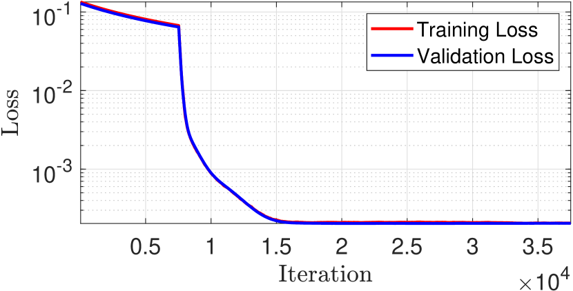
Figure 3: Simple pendulum. Training and validation loss on a logarithmic scale to approximate the simple pendulum system.

Next, the trained neural network and the neural filter are used to predict the state of the pendulum system. In particular, we set $x(0)=\begin{bmatrix}\frac{\pi}{3}&1\end{bmatrix}^{\rm T}.$ In the neural filter, we set $P(0)=10^{-4}\times I_{2},$ where $I_{2}$ is the 2 by 2 identity matrix. Figure 4 shows the predicted states using the neural network (subfigures in the left column) and the neural filter (subfigures in the right column). Note that the state predictions using the neural network degrade over time, as shown by the increasing state error norm $\|e_{k|k}\|$ and the trace of the corresponding state covariance ${\rm tr}\,P_{k|k}.$ On the other hand, the state predictions using the neural filter remain accurate over time, as shown by the bounded state error norm $\|e_{k|k}\|$ and the trace of the corresponding state covariance ${\rm tr}\,P_{k|k}.$

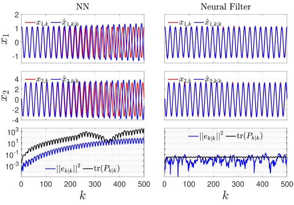
Figure 4: Simple pendulum. State predictions using the neural network and the neural filter.

III-B Van Der Pol

Consider the Van Der Pol oscillator

$$\ddot{q}-\mu(1-q^{2})\dot{q}+q=0.$$ (19)

Defining $x\stackrel{{\scriptstyle\triangle}}{{=}}\begin{bmatrix}q&\dot{q}\end{bmatrix}^{\rm T},$ the Van der Pol oscillator (19) can be written in the state-space form (14), where

$$f(x)\stackrel{{\scriptstyle\triangle}}{{=}}\begin{bmatrix}x_{2}\\ \mu(1-{x_{1}}^{2})x_{2}-x_{1}\end{bmatrix}.$$ (20)

The training data consists of 30,000 samples of $x(0)\in\begin{bmatrix}{\mathcal{U}}[-5,5]\\ {\mathcal{U}}[-5,5]\end{bmatrix}.$ Using MATLAB’s ode45 routine, $x(0.1)$ is computed according to (15). In this work, we use 80 $\%$ of the data to train the model, and the remaining 20 $\%$ are used for validation during the training process.

The neural network architecture used to approximate the Van der Pol oscillator is shown in Figure 5. In particular, the neural network consists of an input layer with a dimension of 2, two hidden layers containing 10 neurons each, and an output layer with a dimension of 2. Both hidden layers use the rectified linear unit (ReLU) activation function, while the output layer uses a linear activation function. The Adam optimizer is used for training the neural network. Training is performed with a batch size of 32, and validation is conducted every 30 iterations. Figure 6 shows the smoothed training and validation loss on logarithmic scale during the training process.

Figure 5: Structure of the neural network trained on the Van der Pol oscillator.

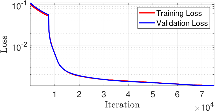
Figure 6: Van der Pol oscillator. Smoothed training and validation loss on logarithmic scale during the training process.

Next, the trained neural network and the neural filter are used to predict the state of the Van der Pol oscillator. In particular, we set $x(0)=\begin{bmatrix}2&1\end{bmatrix}^{\rm T}.$ In the neural filter, we set $P(0)=10^{-4}\times I_{2},$ where $I_{2}$ is the 2 by 2 identity matrix. Figure 7 shows the predicted states using the neural network (subfigures in the left column) and the neural filter (subfigures in the right column). Note that the state predictions using the neural network degrade over time, as shown by the increasing state error norm $\|e_{k|k}\|$ and the trace of the corresponding state covariance ${\rm tr}\,P_{k|k}.$ On the other hand, the state predictions using the neural filter remain accurate over time, as shown by the bounded state error norm $\|e_{k|k}\|$ and the trace of the corresponding state covariance ${\rm tr}\,P_{k|k}.$

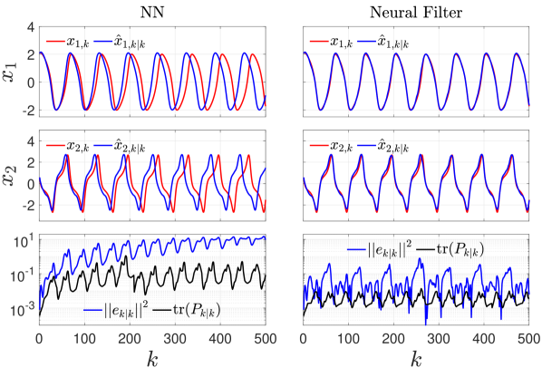
Figure 7: Van der Pol oscillator. State predictions using the neural network and the neural filter.

III-C Lorenz System

Consider the Lorenz system

$$\dot{w} =\sigma(y-w),$$

$$\dot{y} =w(\rho-z)-y,$$

$$\dot{z} =wy-\beta z.$$ (21)

Defining $x\stackrel{{\scriptstyle\triangle}}{{=}}\begin{bmatrix}w&y&z\end{bmatrix}^{\rm T},$ the Lorenz system (III-C) can be written in the state-space form (14), where

$$f(x)\stackrel{{\scriptstyle\triangle}}{{=}}\begin{bmatrix}\sigma(x_{2}-x_{1})\\ x_{1}(\rho-x_{3})-x_{2}\\ x_{1}x_{2}-\beta x_{3}\end{bmatrix}.$$ (22)

The training data consists of 100,000 samples of $x(0)\in\begin{bmatrix}{\mathcal{U}}[-15,15]\\ {\mathcal{U}}[-15,15]\\ {\mathcal{U}}[-15,15]\end{bmatrix}.$ Using MATLAB’s ode45 routine, $x(0.01)$ is computed according to (15). In this work, we use 80 $\%$ of the data to train the model, and the remaining 20 $\%$ are used for validation during the training process.

The neural network architecture used to approximate the Lorenz system is shown in Figure 8. In particular, the neural network consists of an input layer with a dimension of 3, three hidden layers containing 10 neurons each, and an output layer with a dimension of 3. All the hidden layers use the rectified linear unit (ReLU) activation function, while the output layer uses a linear activation function. The Adam optimizer is used for training the neural network. Training is performed with a batch size of 32, and validation is conducted every 30 iterations. Figure 9 shows the smoothed training and validation loss on logarithmic scale during the training process.

Figure 8: Structure of the neural network trained on the Lorenz system.

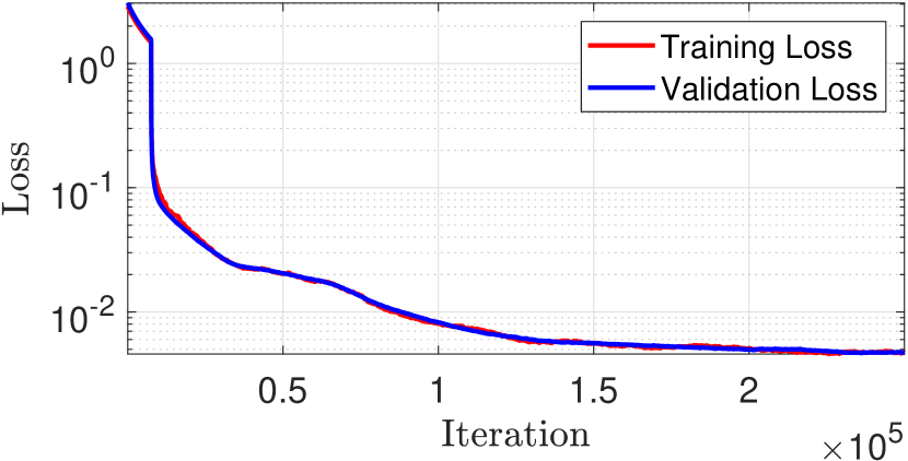
Figure 9: Lorenz system. Smoothed training and validation loss on logarithmic scale during the training process.

Next, the trained neural network and the neural filter are used to predict the state of the Lorenz system. In particular, we set $x(0)=\begin{bmatrix}-6.13&1.78&1.67\end{bmatrix}^{\rm T}.$ In the neural filter, we set $P(0)=10^{-4}\times I_{3},$ where $I_{3}$ is the 3 by 3 identity matrix. Figure 10 shows the predicted states using the neural network (subfigures in the left column) and the neural filter (subfigures in the right column). Note that the state predictions using the neural network degrade over time, as shown by the increasing state error norm $\|e_{k|k}\|$ and the trace of the corresponding state covariance ${\rm tr}\,P_{k|k}.$ On the other hand, the state predictions using the neural filter remain accurate over time, as shown by the bounded state error norm $\|e_{k|k}\|$ and the trace of the corresponding state covariance ${\rm tr}\,P_{k|k}.$

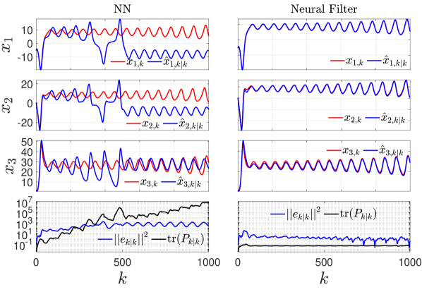
Figure 10: Lorenz system. State predictions using the neural network and the neural filter.

III-D Double Inverted Pendulum System

As shown in Figure 11, a planar double simple pendulum consists of particles $y_{1}$ and $y_{2}$ with masses $m_{1}$ and $m_{2},$ respectively. The particle $y_{1}$ is connected to a frictionless pin joint at the point $w$ in the ceiling by means of the massless link ${\mathcal{L}}_{1}$ with length $\ell_{1},$ and the particle $y_{2}$ is connected by a frictionless pin joint at $y_{1}$ to the first link by means of the massless link ${\mathcal{L}}_{2}$ with length $\ell_{2}.$ The external torque $\tau_{\rm ext}$ is applied to link ${\mathcal{L}}_{1}.$

Figure 11: Planar double simple pendulum.

The equations of motion of the double pendulum are

$$(m_{2}+m_{1})\ell_{1}^{2}\ddot{\theta}_{1} +m_{2}\ell_{1}\ell_{2}(\cos\phi)\ddot{\theta}_{2}=m_{2}\ell_{1}\ell_{2}(\sin\phi)\dot{\theta}_{2}^{2}$$

$$\quad-(m_{1}+m_{2})g\ell_{1}\sin\theta_{1}+\tau_{\rm ext},$$ (23)

$$\ell_{1}(\cos\phi)\ddot{\theta}_{1} +\ell_{2}\ddot{\theta}_{2}=-\ell_{1}(\sin\phi)\dot{\theta}_{1}^{2}-g\sin\theta_{2},$$ (24)

where $\phi\stackrel{{\scriptstyle\triangle}}{{=}}\theta_{2}-\theta_{1}.$

The equations of motion can be written compactly as

$${\mathcal{M}}(\theta)\ddot{\theta}+{\mathcal{D}}(\theta,\dot{\theta})=T,$$ (25)

where $\theta\stackrel{{\scriptstyle\triangle}}{{=}}\begin{bmatrix}\theta_{1}\\ \theta_{2}\end{bmatrix}$ and

$${\mathcal{M}}(\theta) \stackrel{{\scriptstyle\triangle}}{{=}}\begin{bmatrix}(m_{2}+m_{1})\ell_{1}^{2}&m_{2}\ell_{1}\ell_{2}(\cos\phi)\\ \ell_{1}(\cos\phi)&\ell_{2}\end{bmatrix},$$ (26)

$${\mathcal{D}}(\theta,\dot{\theta}) \stackrel{{\scriptstyle\triangle}}{{=}}\begin{bmatrix}-m_{2}\ell_{1}\ell_{2}(\sin\phi)\dot{\theta}_{2}^{2}+(m_{1}+m_{2})g\ell_{1}\sin\theta_{1}\\ \ell_{1}(\sin\phi)\dot{\theta}_{1}^{2}+g\sin\theta_{2}\end{bmatrix},$$ (27)

$$T \stackrel{{\scriptstyle\triangle}}{{=}}\begin{bmatrix}\tau_{\rm ext}\\ 0\end{bmatrix}.$$ (28)

The training data consists of 200,000 samples of $x(0)\in\begin{bmatrix}{\mathcal{U}}[-\pi/2,\pi/2]\\ {\mathcal{U}}[-0.5,0.5]\\ {\mathcal{U}}[-\pi/2,\pi/2]\\ {\mathcal{U}}[-0.5,0.5]\end{bmatrix}.$ Using MATLAB’s ode45 routine, $x(0.01)$ is computed according to (15) assuming $\tau_{\rm ext}=0$. In this work, we use 80 $\%$ of the data to train the model, and the remaining 20 $\%$ are used for validation during the training process.

The neural network architecture used to approximate the double pendulum system is shown in Figure 12. In particular, the neural network consists of an input layer with a dimension of 4, four hidden layers containing 10 neurons each, and an output layer with a dimension of 4. All the hidden layers use the rectified linear unit (ReLU) activation function, while the output layer uses a linear activation function. The Adam optimizer is used for training the neural network. Training is performed with a batch size of 32, and validation is conducted every 30 iterations. Figure 13 shows the smoothed training and validation loss on a logarithmic scale during the training process.

Figure 12: Structure of the neural network trained on the double pendulum system.

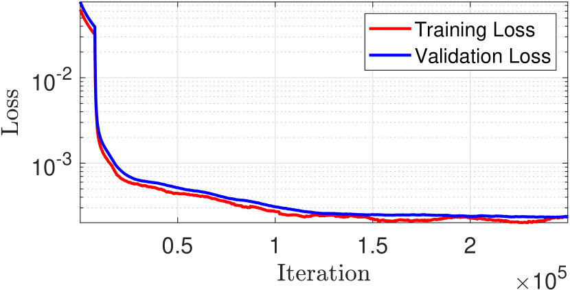
Figure 13: Double pendulum. Smoothed training and validation loss on logarithmic scale during the training process.

Next, the trained neural network and the neural filter are used to predict the state of the double pendulum system. In particular, we set $x(0)=\begin{bmatrix}-0.235&0.267&-0.435&-0.301\end{bmatrix}^{\rm T}.$ In the neural filter, we set $P(0)=10^{-4}\times I_{4},$ where $I_{4}$ is the 4 by 4 identity matrix. Figure 14 shows the predicted states using the neural network (subfigures in the left column) and the neural filter (subfigures in the right column). Note that the state predictions using the neural network degrade over time, as shown by the increasing state error norm $\|e_{k|k}\|$ and the trace of the corresponding state covariance ${\rm tr}\,P_{k|k}.$ On the other hand, the state predictions using the neural filter remain accurate over time, as shown by the bounded state error norm $\|e_{k|k}\|$ and the trace of the corresponding state covariance ${\rm tr}\,P_{k|k}.$

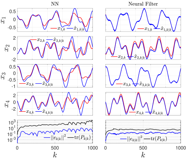
Figure 14: Double pendulum. State predictions using the neural network and the neural filter.

IV Conclusions

This paper introduced the neural filter to improve the accuracy of state predictions using neural network-based models of dynamical systems. Motivated by the extended Kalman filter, the neural filter is constructed using the neural network-based approximation of the dynamical system and augmenting the state prediction by a correction step. The performance of the neural filter is investigated using four nonlinear dynamical systems. In particular, a simple pendulum, a Van der Pol oscillator, Lorenz system, and a double pendulum system are considered to demonstrate the application of the neural filter. In each case, the states predicted by the neural filter are more accurate than the states predicted by the neural network. Furthermore, the covariance of the state estimate given by the neural filter remains bounded, whereas the covariance of the state estimate given by the neural network diverges.

References

[1]Linhao Song, Jun Fan, Di-Rong Chen and Ding-Xuan Zhou
“Approximation of nonlinear functionals using deep ReLU networks”
In Journal of Fourier Analysis and Applications29.4Springer, 2023, pp. 50
[2]Irina Higgins
“Generalizing universal function approximators”
In Nature Machine Intelligence3.3Nature Publishing Group UK London, 2021, pp. 192–193
[3]SF Masri, AG Chassiakos and TK Caughey
“Identification of nonlinear dynamic systems using neural networks”, 1993
[4]Kumpati S Narendra and Kannan Parthasarathy
“Neural networks and dynamical systems”
In International Journal of Approximate Reasoning6.2Elsevier, 1992, pp. 109–131
[5]Kenghong Lin, Xutao Li, Yunming Ye, Shanshan Feng, Baoquan Zhang, Guangning Xu and Ziye Wang
“Spherical Neural Operator Network for Global Weather Prediction”
In IEEE Transactions on Circuits and Systems for Video TechnologyIEEE, 2023
[6]Leonid N Yasnitsky, Andrey A Dumler, Fedor M Cherepanov, Vitaly L Yasnitsky and Natalia A Uteva
“Capabilities of neural network technologies for extracting new medical knowledge and enhancing precise decision making for patients”
In Expert Review of Precision Medicine and Drug Development7.1Taylor & Francis, 2022, pp. 70–78
[7]Lu Lu, Pengzhan Jin and George Em Karniadakis
“Deeponet: Learning nonlinear operators for identifying differential equations based on the universal approximation theorem of operators”
In arXiv preprint arXiv:1910.03193, 2019
[8]Maziar Raissi, Paris Perdikaris and George E Karniadakis
“Physics-informed neural networks: A deep learning framework for solving forward and inverse problems involving nonlinear partial differential equations”
In Journal of Computational physics378Elsevier, 2019, pp. 686–707
[9]Shaowu Pan and Karthik Duraisamy
“Long-time predictive modeling of nonlinear dynamical systems using neural networks”
In Complexity2018.1Wiley Online Library, 2018, pp. 4801012
[10]Katarzyna Michałowska, Somdatta Goswami, George Em Karniadakis and Signe Riemer-Sørensen
“Neural operator learning for long-time integration in dynamical systems with recurrent neural networks”
In arXiv preprint arXiv:2303.02243, 2023
[11]Nima Mohajerin and Steven L Waslander
“Multistep prediction of dynamic systems with recurrent neural networks”
In IEEE transactions on neural networks and learning systems30.11IEEE, 2019, pp. 3370–3383
[12]Charles K Chui and Guanrong Chen
“Kalman filtering”
Springer, 2017
[13]Maria Isabel Ribeiro
“Kalman and extended kalman filters: Concept, derivation and properties”
In Institute for Systems and Robotics43.46Lisboa, Portugal:, 2004, pp. 3736–3741
[14]Bogdan M Wilamowski, Nicholas J Cotton, Okyay Kaynak and GÜnhan Dundar
“Computing gradient vector and Jacobian matrix in arbitrarily connected neural networks”
In IEEE Transactions on Industrial Electronics55.10IEEE, 2008, pp. 3784–3790
[15]William Ditto and Toshinori Munakata
“Principles and applications of chaotic systems”
In Communications of the ACM38.11ACM New York, NY, USA, 1995, pp. 96–102