Reduced Order Hysteretic Magnetization Model for Composite Superconductors

Abstract

In this paper, we propose the Reduced Order Hysteretic Magnetization (ROHM) model to describe the magnetization and instantaneous power loss of composite superconductors. Once the parameters of the ROHM model are fixed based on reference simulations, it allows to directly compute the macroscopic response of composite superconductors without having to solve for the detailed current density distribution. It can be used as a homogenized model in large-scale superconducting systems in order to significantly reduce the computational work compared to detailed simulations. In this contribution, we focus on the case of a strand with twisted superconducting filaments subject to an external transverse magnetic field. We propose two levels of ROHM models: a rate-independent model that reproduces pure hysteresis without dynamic effects, and a rate-dependent model that generalizes the former by also reproducing dynamic effects observed in superconducting strands due to coupling and eddy currents. We describe the implementation and inclusion of these models in a finite element framework, discuss their parameter identification and finally demonstrate the capabilities of the approach in terms of accuracy and efficiency.

Keywords: Reduced Order Method, Hysteresis Model, AC Loss, Magnetization.

1 Introduction

Large-scale superconducting systems are multi-scale structures made of a high number of wounded superconducting cables, which themselves consist of multifilamentary strands or complex arrangements of tapes. The magnetic response of these systems is hysteretic and rate-dependent. Hysteresis is created by the irreversible motion of flux vortices among pinning centers in superconducting parts [1, 2, 3, 4], whereas rate-dependency is caused by eddy currents, and coupling current dynamics between different conductors [5, 6, 7].

Hysteresis, eddy current, and coupling current effects induce loss in transient regimes [5] as well as field distortions [8]. Their computation is therefore crucial, e.g., for computing the load on the cryogenic system, the temperature and stability margins, field errors, or for the design of quench protection devices.

Most approaches to describe the superconducting hysteresis are based on the definition of a relationship between electric field and current density, either non-smooth, as in the Bean model [1], or smooth, as in the power law model [9]. The use of the power law model leads to very accurate results and versatile numerical models with, e.g., the finite element (FE) method [10], which can also be combined with eddy current and coupling current models.

Besides these advantages, the power law introduces a strong nonlinearity in the equations, which makes the numerical models computationally demanding to solve, already for single strands or cables [11]. As a consequence, modelling large-scale superconducting systems in all their details down to the conductor level is completely unrealistic in practice. Faster, more efficient, methods are necessary.

Homogenization methods which reproduce the macroscopic effects of coupling dynamics without modelling them explicitly are good candidates. The general idea of these methods is to describe the systems in terms of the average fields [12], in order to reproduce the magnetization and loss accurately, without having to solve for the detailed current density distribution, which has the potential to strongly reduce the computational cost of the simulations.

Such techniques have been extensively studied in non-superconducting electromagnetic systems, such as periodical structures [13, 14, 15] with bundles of wires of any shape, described in the frequency or time domain [16, 17]. They rely on the design of equivalent conductivity and permeability parameters, that must be fitted on reference solutions, or on experimental measurement results.

Following a similar approach for superconducting systems requires to use dedicated history-dependent parameters in order to reproduce their hysteretic response.

A few hysteresis models have been proposed for modelling superconductor. A vector model is proposed in [8, 18] for field quality computation in accelerator magnets. This model describes the magnetization of superconducting filaments using nested magnetization ellipses. Another hysteresis model based on the Preisach model [19] was proposed in [20, 21] in the form of an equivalent circuit element. Yet another vector model based on a variational approach was described in [22]. These models however only describe rate-independent hysteresis and are therefore not suited for modelling transient effects in composite superconductors.

The literature on hysteresis models for ferromagnetic materials is much more extensive. Among the most popular models are the Jiles-Atherton [23], Preisach [19] models, and rate-dependent models such as the Chua-Stromsmoe model [24, 25]. In 1997, Bergqvist proposed a thermodynamically consistent approach to model hysteresis [26], which led to the development of the energy-based model [27, 28, 29].

The energy-based model offers several advantages. First, it gives a direct access to instantaneous dissipated and stored power by conveniently separating the magnetic field into several contributions. Second, it offers a high flexibility and modularity thanks to an approach involving several sub-elements that can be combined. Third, it is consistently defined as a vector, and not scalar, model from the beginning [27]. Fourth, it can be directly generalized to include rate-dependent effects [28]. Finally, the equations of this model consist in simple explicit tests, which lead to straightforward implementations and very efficient simulations.

In this paper, we adapt and extend the state-of-the-art energy-based model to composite superconductor hysteresis by focussing on the case of a superconducting multifilamentary strand subject to a transverse magnetic field, i.e., a field perpendicular to the strand axis. This situation is relevant for most applications and constitutes a first step towards the homogenization of a complete magnet winding. This is also a challenging problem since, in addition to the filament hysteresis effect, it also involves two types of rate-dependent effects: eddy currents in normal conductors and interfilamentary coupling currents. For this paper, we assume that the strand carries no transport current. The inclusion of transport current will be the focus of further work. We also consider a constant temperature and do not model thermal effects.

We propose two models: (i) a rate-independent model which describes the superconducting hysteresis, and (ii) a rate-dependent model, which generalizes the first model by also describing the eddy current and coupling current effects, in addition to the superconducting hysteresis.

The models are general and can be adapted to a variety of composite superconductors, such as strands, tapes, or cables. They can also be easily implemented in any FE framework allowing for user-defined material properties.

This paper is structured as follows. In Section 2, we introduce the model of a multifilamentary strand and describe its response in terms of magnetization and loss for transverse fields in a range of frequencies and amplitudes. In Section 3, we present the equations leading to rate-independent and rate-dependent hysteresis models. In Section 4, we discuss the implementation of the equations and describe how to include them in a two-dimensional (2D) FE framework with a $\phi$-formulation. We then propose in Section 5 a parameter identification procedure for the models. Finally, in Sections 6 and 7, we apply the hysteresis models in rate-independent and rate-dependent situations, respectively, and demonstrate their potential in the context of homogenization techniques.

2 Multifilamentary Strand Dynamics

In this section, we present the response of a composite multifilamentary superconducting strand subject to a transverse magnetic field in terms of power loss and magnetization. To this end, we model the detailed current density distribution inside the strand with a FE method and we analyze the different dynamics that result from the strand composite structure.

2.1 Problem definition

We consider a strand of diameter $d$ represented in Fig. 1. It consists of $N_{\text{f}}$ Nb-Ti filaments twisted with twist pitch length $p$ and embedded in a conducting copper (Cu) matrix. The geometrical parameters of the strand are summarized in Table 1. The strand carries no transport current but is subject to an applied (app) transverse magnetic field $\boldsymbol{h}_{\text{app}}(t)=h_{\text{max}}\sin(2\pi ft)\hat{\boldsymbol{e}}_{y}$ of amplitude $h_{\text{max}}$ (A/m), frequency $f$ (Hz), and direction $\hat{\boldsymbol{e}}_{y}$.

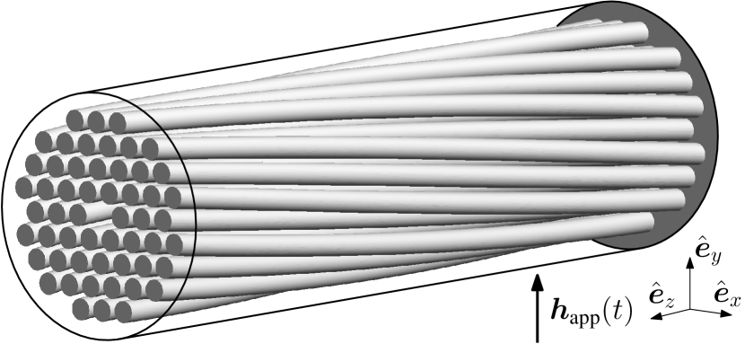
Figure 1: Composite strand with Nb-Ti filaments embedded and twisted in a copper matrix (cylindrical outline) subject to a time-varying transverse magnetic field $\boldsymbol{h}_{\text{app}}(t)$.

Number of filaments ($N_{\text{f}}$)	54
Filament diameter	$90~{}\upmu$m
Filament center-to-center spacing	$110~{}\upmu$m
Strand diameter ($d$)	$1$ mm
Twist pitch length ($p$)	$19$ mm

Table 1: Geometrical parameters of the strand.

We fix the temperature to $1.9$ K. The resistivity of the Nb-Ti filaments is described by the power law [9] with power index $n=30$ and the field-dependent critical current density $j_{\text{c}}(\boldsymbol{b})$ (A/m²) given in Fig. 2, with $\boldsymbol{b}$ (T) the local magnetic flux density, defined as $\boldsymbol{b}=\mu_{0}\boldsymbol{h}$, with $\mu_{0}=4\pi\times 10^{-7}$ H/m the permeability of vacuum. The resistivity of the copper matrix, accounting for magneto-resistance, is obtained from the STEAM material library [30], with a residual resistivity ratio $\text{RRR}=100$.

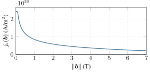
Figure 2: Field-dependent critical current density $j_{\text{c}}(\boldsymbol{b})$. The maximum value is $j_{\text{c}}(\boldsymbol{0})=2.4\times 10^{10}$ A/m².

We model the strand response with the CATI method, proposed in [31]. This method accounts for 3D effects due to the strand twist by using a pair of 2D models solved on a cross section of the strand, and coupled via circuit equations. As it is based on 2D models, it offers fast simulations. The method is implemented in GetDP [32] within FiQuS [33]. FiQuS is developed at CERN as part of the STEAM framework [34]. Geometry and mesh are performed by Gmsh [35]. All the software is open-source and free to use. The code is available online.

2.2 Magnetization and loss

We focus on magnetization and power loss. These are the two quantities we want to reproduce directly with the hysteresis model without having to compute the detailed current density distribution.

The average magnetization vector $\boldsymbol{m}$ (A/m) is defined as the magnetic dipole moment per unit volume [36]. Based on the current density distribution on a given cross section, we have

$$\boldsymbol{m}=2\cdot\frac{1}{2a}\int_{S}\boldsymbol{x}\times\boldsymbol{j}\,\text{d}S,$$ (1)

with $a=\pi d^{2}/4$ the surface area of the strand cross section $S$, $\boldsymbol{x}$ the position vector, and $\boldsymbol{j}$ the current density. The multiplication by $2$ accounts for current loops closing at infinity in this 2D problem, as justified in A.

The instantaneous power loss per unit length $P_{\text{tot}}$ (in W/m) is obtained by integrating the instantaneous power loss density, or Joule loss, over the strand cross section, including the Nb-Ti filaments and the Cu matrix,

$$P_{\text{tot}}=\int_{S}\boldsymbol{j}\cdot\boldsymbol{e}\,\text{d}S,$$ (2)

with $\boldsymbol{e}=\rho\boldsymbol{j}$ the electric field (and $\rho$ the resistivity). The power loss per cycle and per unit length (in J/m) is evaluated as

$$Q_{\text{tot}}=\int_{1/f}^{2/f}P_{\text{tot}}(t)\,dt.$$ (3)

To make the interpretation of the loss easier, and also because it will be helpful for the construction of the hysteresis model, the total power loss per cycle $Q_{\text{tot}}$ is decomposed in three contributions, as was done in [31]: hysteresis, coupling, and eddy loss. The hysteresis loss is the loss induced by currents flowing in the superconducting filaments. The coupling loss is the loss induced by currents flowing in the conducting matrix, perpendicular to $\hat{\boldsymbol{e}}_{z}$ (the coupling currents). Finally, the eddy loss is the loss induced by currents flowing in the conducting matrix along $\hat{\boldsymbol{e}}_{z}$.

Magnetization and loss are closely related to each other. Indeed, the area inside a closed magnetization loop is proportional to the total loss per cycle [37, 38]. We have, in terms of the applied magnetic field $\boldsymbol{h}_{\text{app}}$,

$$Q_{\text{tot}}=a\oint\mu_{0}\boldsymbol{h}_{\text{app}}\cdot\text{d}\boldsymbol{m}.$$ (4)

2.3 Dynamic response of the strand

The strand response is computed by the CATI method for a range of field amplitudes $h_{\text{max}}$ and frequencies $f$. The power loss per cycle induced by the transverse field is represented in Fig. 3 as a function of $f$ for three different values of $h_{\text{max}}$. The $y$-component of the magnetization vector, $m$, is represented in Figs. 4 and 5 for $\mu_{0}h_{\text{max}}=2$ T as a function of $\mu_{0}h_{\text{app}}(t)$ for selected frequencies.

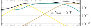
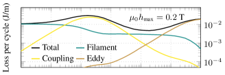
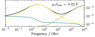
Figure 3: Total loss per cycle and its contributions as a function of the frequency $f$, for three different magnetic field amplitudes. The legend is the same for the three subfigures. Results from [31].

At low frequencies, when the rate of change of the transverse magnetic field is not high enough for significant coupling currents and eddy currents to take place in the matrix, the superconducting filaments behave close to uncoupled. In that regime, most loss is due to hysteresis in the filaments. A typical magnetization loop in that case is represented in Fig. 4. The magnetization decreases when the field increases as a result of the field-dependent critical current density. In this regime, a good first approximation is to consider that the response is rate-independent (it is not strictly the case in reality due to the finite value of the $n$ index in the power law). To this end, a rate-independent hysteresis model can be used.

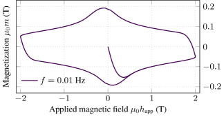
Figure 4: Strand magnetization along $\hat{\boldsymbol{e}}_{y}$ for $\mu_{0}h_{\text{max}}=2$ T and $f=0.01$ Hz. Same result as the first curve in Fig. 5.

When the frequency increases, the response of the strand becomes strongly rate-dependent. As shown in Fig. 3, coupling and eddy loss can dominate the total loss, and the filament loss is not constant with frequency. As a result, the loss per cycle can exhibit more than one order of magnitude of variation as a function of frequency for an identical applied field amplitude. Similarly, the magnetization strongly depends on the frequency, as shown in Fig. 5. To reproduce these regimes, there is a clear need for a rate-dependent hysteresis model. The design of such a model benefits from a good understanding of the physics of the curves in Figs. 3 and 5.

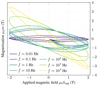
Figure 5: Strand magnetization for $\mu_{0}h_{\text{max}}=2$ T and for different frequencies $f$. Results from [31] using Eq. (1).

For low field amplitudes, the dynamics of the coupling currents and of the associated loss is well described by analytical models [5, 39]. The coupling loss follows follows a typical bell curve with a maximum at a characteristic frequency $f_{\text{c}}$.

With increasing field amplitude, the peak of the coupling loss curve shifts towards lower frequencies, as can be seen in Fig. 3 for $\mu_{0}h_{\text{max}}=2$ T. This is associated with the saturation of superconducting filaments, which limit the coupling currents amplitude, and to a change of the effective permeability, due to the loss of diamagnetic effect due to saturated filaments, as discussed in [5].

The coupling currents also give rise to a change of regime for the filament magnetization and loss. As mentioned previously, at low frequencies, $f\lesssim f_{\text{c}}$, they are mostly uncoupled, producing a relatively small magnetization. On the other hand, for $f\gtrsim f_{\text{c}}$, they are coupled and exchange currents via coupling currents. As a result, their magnetization is increased, see for example the situation for $f=10$ Hz in Fig. 5. Whether the filament loss for coupled filaments is higher or lower than that for uncoupled filaments depends on $\mu_{0}h_{\text{max}}$, as can be seen in Fig. 3.

At even higher frequencies, eddy currents in the conducting matrix become the dominating factor for loss and magnetization. As a result of eddy currents and the skin effect, the inner part of the strand, containing the filaments, is shielded from the outer field and the filament loss decreases accordingly. In that regime, the magnetization curve approaches the shape of an ellipse [37] that gets thinner and thinner with increasing frequency, and of slope approaching $-2$ because of demagnetization effects (this is further explained in Section 3.1) [38].

3 Reduced Order Hysteretic Magnetization Model

The simulation time for each of the simulations presented in the previous section is of the order of one hour with the CATI method. This is fast and convenient enough to get a good understanding of a single strand response. However, for simulating a full-scale magnet, containing thousands of strands, one cannot afford such a detailed description of the current density at the strand level. Instead, one has to use an alternative model that produces similar macroscopic response in terms of power loss and magnetization, which are both history-dependent and rate-dependent, but without requiring a detailed calculation of the current density, so as to strongly reduce the computational cost. This idea is illustrated in Fig. 6. We present such a model in this section, the Reduced Order Hysteretic Magnetization (ROHM) model.

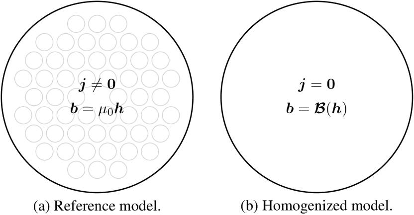
Figure 6: Illustration of the homogenization concept with no transport current. It consists of defining a rate-dependent hysteretic relationship $\boldsymbol{b}=\boldsymbol{\mathcal{B}}(\boldsymbol{h})$ in a homogenized material without modelling any current density. The relationship should be carefully designed in such a way that it leads to equivalent magnetization, i.e., an equivalent effect on the outside field, and equivalent power loss compared to the reference solution.

This model is adapted and inspired from the energy-based model for ferromagnetic materials [27, 28].

We start in Section 3.1 by clarifying how the ROHM model can be used to model the strand. We then define the building blocks, referred to as cells, that will be combined for the construction of the model. Each cell defines a local hysteretic relationship between the magnetic field $\boldsymbol{h}$ and the magnetic flux density $\boldsymbol{b}$. We present in Section 3.2 a rate-independent cell, that we call the superconductor cell (S cell). In Section 3.3, we add contributions to account for eddy current and coupling current effects, resulting in a rate-dependent cell, that we call the composite superconductor cell (CS cell). In Section 3.4, we discuss how to reproduce the effect of a field-dependent critical current density within the cells. Finally, we show in Section 3.5 how several cells can be combined into a chains of cell, defining a complete ROHM model.

3.1 Concept of a reduced order model

The idea is to replace the detailed cross section of the strand by a plain, homogenized, material. Such a material is assumed to be not conducting, but magnetic, and is described by a constitutive law $\boldsymbol{b}=\boldsymbol{\mathcal{B}}(\boldsymbol{h})$ between the local magnetic field $\boldsymbol{h}$ and the local magnetic flux density $\boldsymbol{b}$. The constitutive law is designed to produce a magnetization vector and power loss value that are equivalent to those obtained with the detailed reference model [37].

With fields $\boldsymbol{b}$ and $\boldsymbol{h}$ that satisfy $\boldsymbol{b}=\boldsymbol{\mathcal{B}}(\boldsymbol{h})$, the magnetization vector $\boldsymbol{m}$ (in A/m) is defined by [37]:

$$\boldsymbol{b}=\mu_{0}\boldsymbol{h}+\mu_{0}\boldsymbol{m}.$$ (5)

Similarly, the power loss is no longer obtained via a current density as in Eq. (2), but is now instead described by the magnetic power density $\boldsymbol{h}\cdot\dot{\boldsymbol{b}}$. Part of this power is related to stored magnetic energy, and hence not associated with loss, and the remaining part is related to dissipated energy. One major advantage of the energy-based hysteresis model used in this work is that it gives access to both parts separately at any time [27].

The relationship $\boldsymbol{b}=\boldsymbol{\mathcal{B}}(\boldsymbol{h})$ is written in terms of the local fields $\boldsymbol{h}$ and $\boldsymbol{b}$, internal to the strand. Because of the demagnetization effect, the internal magnetic field $\boldsymbol{h}$ is not equal to the applied field $\boldsymbol{h}_{\text{app}}$. In the case of a round strand subject to a transverse external field, the demagnetization factor is equal to $1/2$ and we have [38]:

$$\boldsymbol{h}=\boldsymbol{h}_{\text{app}}-\frac{1}{2}\boldsymbol{m}.$$ (6)

For this reason, the magnetization curves produced by the hysteresis model $\boldsymbol{b}=\boldsymbol{\mathcal{B}}(\boldsymbol{h})$ are not to be compared with those depicted in Figs. 4 and 5, but rather with different ones, drawn as a function of

$$\boldsymbol{h}_{\text{in}}=\boldsymbol{h}_{\text{app}}-\frac{1}{2}\boldsymbol{m},$$ (7)

where $\boldsymbol{h}_{\text{in}}$ has no immediate meaning in the detailed strand model per se, but is the local magnetic field the hysteresis model will see inside the strand. These curves are shown in Fig. 7. At high frequencies ($f\gtrsim 10^{4}$ Hz), they approach the shape of an ellipse with a slope of $-1$. The area of closed loops are identical in both Figs. 5 and 7, as shown in B.

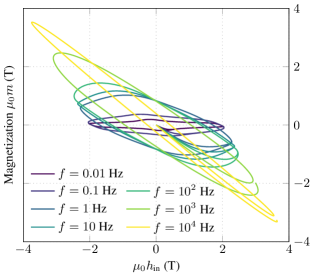
Figure 7: Strand magnetization for $\mu_{0}h_{\text{max}}=2$ T. Same results as in Fig. 5 but in terms of $\mu_{0}h_{\text{in}}$ instead of $\mu_{0}h_{\text{app}}$ (see Eq. (7)).

3.2 Superconductor cell - S cell

As a first step, we present a rate-independent hysteresis cell [27], that we refer to as the superconductor cell, or S cell. In this cell, the magnetic field $\boldsymbol{h}$ is decomposed into a reversible field, $\boldsymbol{h}_{\text{rev}}$, and an irreversible field, $\boldsymbol{h}_{\text{irr}}$:

$$\boldsymbol{h}=\boldsymbol{h}_{\text{rev}}+\boldsymbol{h}_{\text{irr}}.$$ (8)

The reversible field defines the magnetic flux density:

$$\boldsymbol{b}=\mu_{0}\boldsymbol{h}_{\text{rev}}.$$ (9)

The irreversible field creates hysteresis by introducing history dependence. Its amplitude $\|\boldsymbol{h}_{\text{irr}}\|$ is bounded by a value $\kappa$ (A/m), the irreversibility parameter. From a known magnetic field $\boldsymbol{h}$, which is the driving vector, and a given reversible field $\boldsymbol{h}_{\text{rev}}$ that has been established previously (as a function of the history of $\boldsymbol{h}$), the irreversible field $\boldsymbol{h}_{\text{irr}}$ is determined as follows:

$$\boldsymbol{h}_{\text{irr}} =\left\{\begin{aligned} &\boldsymbol{h}-\boldsymbol{h}_{\text{rev}},\quad&&\text{if }\|\boldsymbol{h}-\boldsymbol{h}_{\text{rev}}\|<\kappa,\\ &\kappa\ \dot{\boldsymbol{b}}/\|\dot{\boldsymbol{b}}\|,\quad&&\text{if }\|\boldsymbol{h}-\boldsymbol{h}_{\text{rev}}\|=\kappa,\\ \end{aligned}\right.$$ (10)

where the dot notation (as in $\dot{\boldsymbol{b}}$) represents the time derivative of the quantity. An illustration of this equation is given in Fig. 8. While the driving field $\boldsymbol{h}$ evolves inside the sphere of radius $\kappa$ centered at $\boldsymbol{h}_{\text{rev}}$, the reversible field $\boldsymbol{h}_{\text{rev}}$ stays constant, and the irreversible field is defined accordingly, see Fig. 8(a). If $\boldsymbol{h}$ reaches the surface of the sphere, then, the reversible field $\boldsymbol{h}_{\text{rev}}$ must evolve as well, in order to maintain the condition $\|\boldsymbol{h}_{\text{irr}}\|\leq\kappa$ valid, and $\boldsymbol{h}_{\text{irr}}$ is established parallel to $\dot{\boldsymbol{b}}$, see Fig. 8(b).

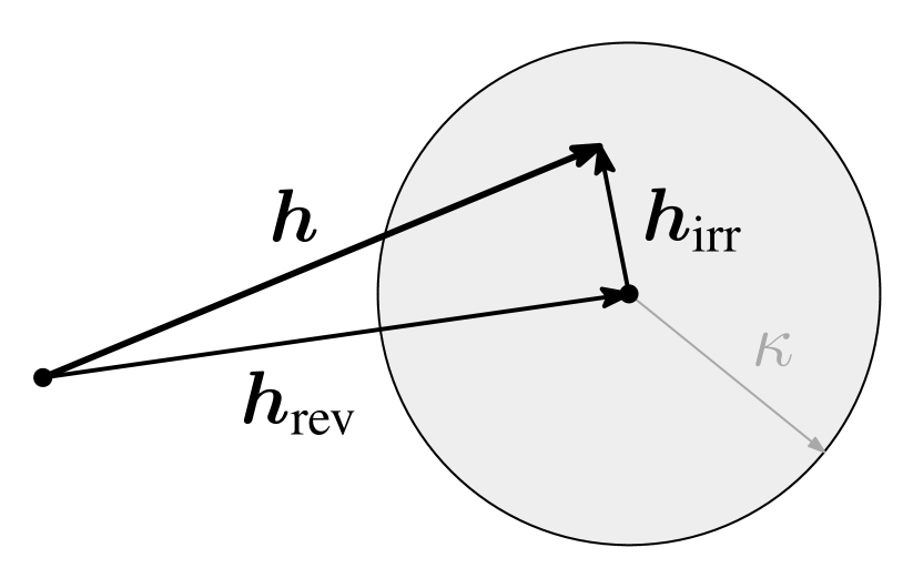
(a) $\|\boldsymbol{h}-\boldsymbol{h}_{\text{rev}}\|<\kappa$.

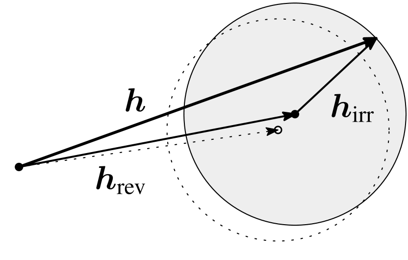
(b) $\|\boldsymbol{h}-\boldsymbol{h}_{\text{rev}}\|=\kappa$.

Figure 8: S cell, adapted from [27, 29]. Illustration of the magnetic field decomposition into reversible and irreversible fields in 2D. The dotted elements in (b) refer to the situation at a previous time.

The total power density $p_{\text{tot}}$ (in W/m³) is expressed as

$$p_{\text{tot}} =\boldsymbol{h}\cdot\dot{\boldsymbol{b}}$$

$$=\underbrace{\boldsymbol{h}_{\text{rev}}\cdot\dot{\boldsymbol{b}}}_{p_{\text{rev}}}+\underbrace{\boldsymbol{h}_{\text{irr}}\cdot\dot{\boldsymbol{b}}}_{p_{\text{irr}}}.$$ (11)

The reversible power $p_{\text{rev}}$ is the time derivative of a stored magnetic energy density,

$$p_{\text{rev}}=\boldsymbol{h}_{\text{rev}}\cdot\mu_{0}\dot{\boldsymbol{h}}_{\text{rev}}=\frac{d}{dt}\left(\frac{1}{2}\boldsymbol{h}_{\text{rev}}\cdot\mu_{0}\boldsymbol{h}_{\text{rev}}\right),$$ (12)

while the irreversible power $p_{\text{irr}}$ is always non-negative and is associated with dissipated energy density,

$$p_{\text{irr}}=\boldsymbol{h}_{\text{irr}}\cdot\dot{\boldsymbol{b}}=\kappa\|\dot{\boldsymbol{b}}\|=\kappa\|\mu_{0}\dot{\boldsymbol{h}}_{\text{rev}}\|.$$ (13)

It is one of the main benefits of the energy-based approach that the dissipated energy is clearly separated from the stored energy [27].

A mechanical analogy of a S cell in a one-dimensional setting is shown in Fig. 9. It represents a mechanical system made of a dry friction element in parallel with a restoring spring [27]. Examples of hysteresis curves computed with the S cell are shown in Fig. 10. These curves are independent of the rate of change of the applied field.

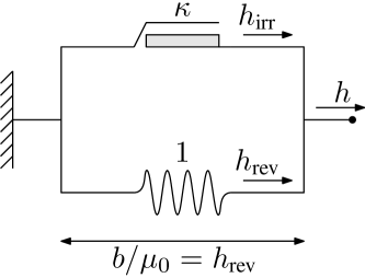
Figure 9: Mechanical analogy [27] of the S cell: a parallel connection of a dry friction element and a restoring spring. The system is subject to a force $h$, which causes an elongation $b=\mu_{0}h_{\text{rev}}$.

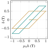
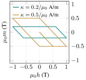
Figure 10: Hysteresis curves for the S cell subject to a unidirectional oscillating magnetic field $h$ as an input. The legend is the same for both subfigures. (Left) Magnetic flux density $b$ versus applied field $\mu_{0}h$. (Right) Magnetization $\mu_{0}m=b-\mu_{0}h$ versus applied field $\mu_{0}h$.

3.3 Composite superconductor cell - CS cell

In regimes in which the superconducting strand response is clearly not rate-independent, the S cell presented in the previous section must be generalized. Starting from the S cell, we propose to account for the magnetization due to eddy currents and coupling currents by adding two new contributions in the magnetic field decomposition, $\boldsymbol{h}_{\text{eddy}}$ and $\boldsymbol{h}_{\text{coupling}}$, such that Eq. (8) is rewritten

$$\boldsymbol{h}=\boldsymbol{h}_{\text{rev}}+\boldsymbol{h}_{\text{irr}}+\boldsymbol{h}_{\text{eddy}}+\boldsymbol{h}_{\text{coupling}}.$$ (14)

The equation for $\boldsymbol{h}_{\text{irr}}$ is modified accordingly:

$$\boldsymbol{h}_{\text{irr}} =\left\{\begin{aligned} &\boldsymbol{h}-\boldsymbol{g},\quad&&\text{if }\|\boldsymbol{h}-\boldsymbol{g}\|<\kappa,\\ &\kappa\ \dot{\boldsymbol{b}}/\|\dot{\boldsymbol{b}}\|,\quad&&\text{if }\|\boldsymbol{h}-\boldsymbol{g}\|=\kappa,\\ \end{aligned}\right.$$ (15)

with $\boldsymbol{g}=\boldsymbol{h}_{\text{rev}}+\boldsymbol{h}_{\text{eddy}}+\boldsymbol{h}_{\text{coupling}}$. The magnetic field decomposition is represented in Fig. 11(b). As described below, the fields $\boldsymbol{h}_{\text{eddy}}$ and $\boldsymbol{h}_{\text{coupling}}$ are always parallel to $\dot{\boldsymbol{b}}=\mu_{0}\dot{\boldsymbol{h}}_{\text{rev}}$. We refer to this new cell as the composite superconductor cell, or CS cell.

Adapting [28], the field $\boldsymbol{h}_{\text{eddy}}$ is defined as

$$\boldsymbol{h}_{\text{eddy}}=\tau_{\text{e}}\dot{\boldsymbol{h}}_{\text{rev}},$$ (16)

with an eddy current time constant parameter $\tau_{\text{e}}$ (s). This component produces a loss contribution, $p_{\text{eddy}}$, which is non-negative. It reads:

$$p_{\text{eddy}}=\boldsymbol{h}_{\text{eddy}}\cdot\dot{\boldsymbol{b}}=\frac{\mu_{0}}{\tau_{\text{e}}}\|\boldsymbol{h}_{\text{eddy}}\|^{2}=\frac{\tau_{\text{e}}}{\mu_{0}}\|\dot{\boldsymbol{b}}\|^{2}.$$ (17)

In the mechanical analogy, the inclusion of eddy current effects corresponds to adding a dashpot (viscous friction element) in parallel with the dry friction element and the restoring spring, as illustrated in Fig. 11(a). For slow variations of the force $h$, the dashpot is barely opposing the elongation $b$, whereas for faster variations of $h$, it becomes gradually more blocking and starts to oppose to variations of $b$. This reproduces magnetic shielding and increased magnetization due to eddy currents.

The next new contribution $\boldsymbol{h}_{\text{coupling}}$ is associated with coupling currents [5]. The coupling currents in the conducting matrix are fed by currents flowing in the superconducting filaments, and are therefore also subject to hysteresis and saturation of the filaments. The field $\boldsymbol{h}_{\text{coupling}}$ has then its own irreversibility parameter $\chi$ (in A/m). We define

$$\boldsymbol{h}_{\text{coupling}} =\left\{\begin{aligned} &\tau_{\text{c}}\dot{\boldsymbol{h}}_{\text{rev}},&&\text{if }\|\tau_{\text{c}}\dot{\boldsymbol{h}}_{\text{rev}}\|<\chi,\\ &\chi\ \dot{\boldsymbol{h}}_{\text{rev}}/\|\dot{\boldsymbol{h}}_{\text{rev}}\|,&&\text{if }\|\tau_{\text{c}}\dot{\boldsymbol{h}}_{\text{rev}}\|\geq\chi.\\ \end{aligned}\right.$$ (18)

$$=\frac{\tau_{\text{c}}}{\mu_{0}}\dot{\boldsymbol{b}}_{\text{coupling}},$$ (19)

with a coupling currents time constant $\tau_{\text{c}}$ (s). The field $\boldsymbol{h}_{\text{coupling}}$ introduces two new loss contributions, $p_{\text{coupling}}$ and $p_{\text{irr,c}}$, that read:

$$p_{\text{coupling}} =\frac{\mu_{0}}{\tau_{\text{c}}}\|\boldsymbol{h}_{\text{coupling}}\|^{2}=\frac{\tau_{\text{c}}}{\mu_{0}}\|\dot{\boldsymbol{b}}_{\text{coupling}}\|^{2},$$ (20)

$$p_{\text{irr,c}} =\boldsymbol{h}_{\text{coupling}}\cdot\left(\dot{\boldsymbol{b}}-\dot{\boldsymbol{b}}_{\text{coupling}}\right).$$ (21)

The mechanical analogy associated with this new problem is represented in Fig. 11(a). The combination of the dashpot in series with the dry friction element reproduces the saturation of the coupling currents. When the force on the dashpot remains below $\chi$, the dry friction element is at rest and produces no hysteresis. This corresponds to a situation in which the coupling currents are small enough for the hysteresis to be neglected. If the force exceeds $\chi$ on the dashpot, it is then subject to hysteresis. The second hysteresis element, with $\chi$, always acts in parallel with the first one, related to filament magnetization. The magnetization of coupled filaments therefore depends of the sum of both.

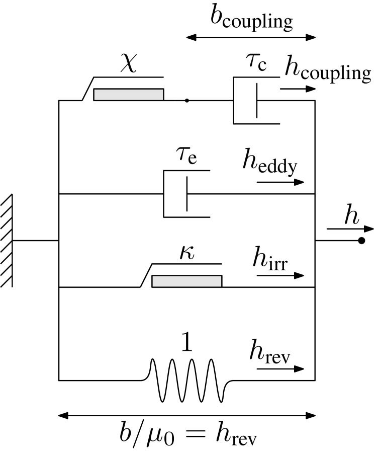
(a) Mechanical analogy.

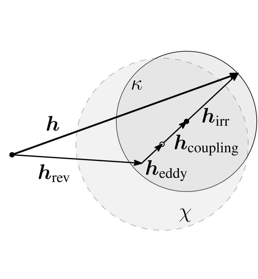
(b) Illustration in 2D.

Figure 11: CS cell accounting for eddy currents and coupling current effects. The dashed circle of radius $\chi$ limits the amplitude of the field $\boldsymbol{h}_{\text{coupling}}$.

Note that by choosing $\tau_{\text{e}}=0$ and $\tau_{\text{c}}=0$, we retrieve the S cell of Section 3.2. The S cell is therefore a particular case of the CS cell.

An illustration of magnetization curves obtained with a CS cell is given in Fig. 12, and the loss per cycle as a function of frequency is given in Fig. 13. The loss per cycle curve exhibits the sought features for the composite strand. The filament curve shows the expected evolution, two plateaus at low and middle frequencies, with a transition where the coupling loss peaks, and then a sharp decrease when the eddy loss becomes dominant. Coupling and eddy loss curves both follow the shape of two bell curves.

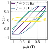
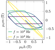
Figure 12: Hysteresis curves for the composite hysteresis cell reproducing eddy and coupling currents, with $\kappa=0.2/\mu_{0}$ A/m, $\chi=0.3/\mu_{0}$ A/m, $\tau_{\text{c}}=0.1$ s, and $\tau_{\text{e}}=70$ $\upmu$s. Unidirectional oscillating magnetic field $h$ as an input. The legend is shared between both subfigures. (Left) Magnetic flux density $b$ versus applied field $\mu_{0}h$. (Right) Magnetization $\mu_{0}m=b-\mu_{0}h$ versus applied field $\mu_{0}h$.

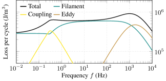
Figure 13: Total loss per cycle and separated loss contributions as a function of the frequency $f$, for a magnetic field amplitude of $2$ T obtained with the same composite hysteresis cell as in Fig. 12.

Note that the eddy current curve for the eddy loss per cycle should be asymptotically decreasing as $1/\sqrt{f}$ at high frequencies, due to the skin effect. With the CS cell, one can however only expect the curve to decrease as $1/f$ at high frequencies. For $f\to\infty$, the CS cell is therefore not expected to provide perfectly valid results. It should be further improved if a more realistic frequency response is wanted in such high frequencies. For most practical applications however, the field rates of change are sufficiently low for this error to stay small.

Comparing with the results from a detailed multifilamentary strand model in Fig. 3, one can see that a single CS cell is still not sufficiently accurate. Several of them have to be combined to achieve a better matching with the reference, as will be discussed in Section 3.5.

3.4 Inclusion of $j_{\text{c}}(b)$ field dependence

In reality, the magnetization of superconductors decreases with increasing field, as a consequence of the decreasing critical current density $j_{\text{c}}$. Such an effect is not yet reproduced with the hysteresis cells defined above, because the irreversibility parameters $\kappa$ and $\chi$ are still constant values. By making the irreversibility parameters $\kappa$ and $\chi$ decrease with increasing field, one can produce more realistic magnetization curves.

In general, we therefore define field-dependent irreversibility parameters:

$$\kappa(\boldsymbol{b})=f_{\kappa}(\boldsymbol{b})\bar{\kappa},\quad\chi(\boldsymbol{b})=f_{\chi}(\boldsymbol{b})\bar{\chi},$$ (22)

with $\bar{\kappa}$ and $\bar{\chi}$ two constants (in A/m) and $f_{\kappa}$ and $f_{\chi}$ two scaling functions, smoothly evolving from $1$ at zero field to $0$ at large fields. The expressions of $f_{\kappa}$ and $f_{\chi}$ are functions of the geometry and must be determined at the parameter identification step. This will be discussed in Section 5.

Note that the introduction of field-dependent irreversibility parameters in the cells brings an additional nonlinearity to the equations to be addressed during the numerical simulation.

3.5 Chain of cells

The S cell and the CS cell contain the necessary ingredients to reproduce the different regimes observed in the multifilamentary strand, but a single cell alone does not provides a faithful description over a wide field range. Indeed, if the applied magnetic field is smaller than $\kappa$, both the S cell and the CS cell produce exactly zero magnetic flux density, and hence no loss. In reality, the evolution towards saturation is smooth and progressive, and not subject to a single threshold $\kappa$, as in Figs. 10 and 12.

To better approach the smooth magnetization curves of Figs. 4 and 5, we can combine several cells into what we call a chain of cells. To this end, we follow the approach proposed in [27].

The approach consists of decomposing the total magnetic flux density $\boldsymbol{b}$ into a number of $N\in\mathbb{N}_{0}$ contributions $\alpha_{k}\boldsymbol{b}_{k}$, with $k=1,\dots,N$. The $\boldsymbol{b}_{k}$ are described by distinct hysteresis cells, with distinct parameter values and the $\alpha_{k}$ are weights associated with each of them. All cells are subject to the same total magnetic field $\boldsymbol{h}$ and contribute to the total magnetic flux density with weight $\alpha_{k}$. We define

$$\boldsymbol{b}=\sum_{k=1}^{N}\alpha_{k}\boldsymbol{b}_{k}=\sum_{k=1}^{N}\alpha_{k}\mu_{0}\boldsymbol{h}_{\text{rev},k},\ \quad\sum_{k=1}^{N}\alpha_{k}=1,$$ (23)

where $\boldsymbol{h}_{\text{rev},k}$ is the reversible field associated with cell $k$. With the mechanical analogy, this corresponds to connecting cells as a chain, i.e., in series, as illustrated in Fig. 14. The power loss is computed cell by cell, in terms of the fractions $\alpha_{k}\dot{\boldsymbol{b}}_{k}$ of the total rate of change $\dot{\boldsymbol{b}}$.

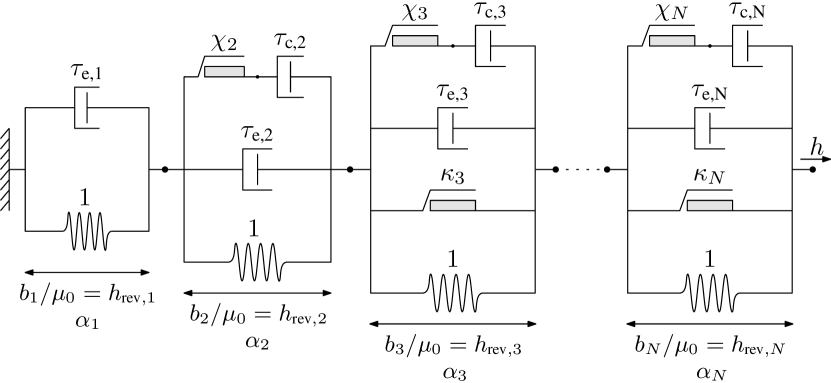
Figure 14: Chain of cells. The total magnetic flux density is computed as $\boldsymbol{b}=\sum_{k=1}^{N}\alpha_{k}\boldsymbol{b}_{k}$. Arbitrary combinations of cells can be put in series. The represented arrangement is relevant for a multifilamentary strand, as explained in Section 7.

The advantage of this approach is that each cell can be solved independently, as they are all subject to the same magnetic field $\boldsymbol{h}$. Fixed point iterations can be performed to account for field-dependent parameters $\kappa$ or $\chi$ that should depend on the total magnetic flux density $\boldsymbol{b}$. The equations for each cell are identical to what was described in Sections 3.2 and 3.3, but each cell only contributes partly to the total magnetic flux density $\boldsymbol{b}$, with a fraction $\alpha_{k}\boldsymbol{b}_{k}$.

Once parameters are identified (see Section 5), the chain of cells defines the hysteresis model, i.e., the constitutive relationship $\boldsymbol{b}=\mathcal{B}(\boldsymbol{h})$ that reproduces the composite strand magnetization and loss.

4 Implementation and Inclusion in FE Framework

The hysteresis model output the magnetic flux density $\boldsymbol{b}(t)$ as a function of a given magnetic field $\boldsymbol{h}(t)$ (from which we can compute the magnetization $\boldsymbol{m}=\boldsymbol{b}/\mu_{0}-\boldsymbol{h}$ and the power loss). Both $\boldsymbol{b}(t)$ and $\boldsymbol{h}(t)$ are vector quantities varying in time. For a numerical simulation, time is discretized and the solutions are sought at successive time steps, based on the knowledge of the solution at previous time steps and on the new value of the magnetic field.

In this section, we first propose update rules for the two types of cells defined in the previous section, the S cell and CS cell. We then discuss the case of a chain of cells and conclude by describing how to include the hysteresis model in a FE framework.

4.1 S cell

If the irreversibility parameter $\kappa$ is constant, the S cell can be solved with an explicit update rule, as proposed in [27]. Let $\boldsymbol{h}_{\text{rev(p)}}$ be the reversible field computed at the previous time step. For a magnetic field $\boldsymbol{h}$, the updated reversible field $\boldsymbol{h}_{\text{rev}}$ reads:

$$\boldsymbol{h}_{\text{rev}} =\left\{\begin{aligned} &\boldsymbol{h}_{\text{rev(p)}},&&\text{if }\|\boldsymbol{h}-\boldsymbol{h}_{\text{rev(p)}}\|\leq\kappa,\\ &\boldsymbol{h}-\kappa\frac{\boldsymbol{h}-\boldsymbol{h}_{\text{rev(p)}}}{\|\boldsymbol{h}-\boldsymbol{h}_{\text{rev(p)}}\|},&&\text{otherwise,}\end{aligned}\right.$$

$$=\boldsymbol{\mathcal{U}}_{\kappa}(\boldsymbol{h},\boldsymbol{h}_{\text{rev(p)}}).$$ (24)

The associated magnetic flux density $\boldsymbol{b}$ is directly given by Eq. (9), and the irreversible field $\boldsymbol{h}_{\text{irr}}$ can be deduced from Eq. (8). The instantaneous rates of stored and dissipated energies, $p_{\text{rev}}$ and $p_{\text{irr}}$, are readily obtained by Eqs. (12) and (13), respectively.

If the irreversibility parameter $\kappa$ is not constant but a function of $\boldsymbol{b}$ as proposed in Section 3.4 to account for field-dependent $j_{\text{c}}$, the update rule is no longer explicit. In such a case however, we observed that a good approximate solution is found easily in a few fixed point iterations, that is, by solving successively Eq. (4.1) with updated values of $\kappa(\boldsymbol{b})=\kappa(\mu_{0}\boldsymbol{h}_{\text{rev}})$ until $\boldsymbol{h}_{\text{rev}}$ does no longer change significantly.

It is remarkable that the implementation of the S cell entirely consists in the simple test of Eq. (4.1). It only requires the knowledge of the previous reversible field, which has to be stored as an internal variable in the numerical implementation.

Note that by contrast with ferromagnetic hysteresis with a nonlinear saturation law [27, 29], in this context of superconducting hysteresis, the relationship Eq. (9) is linear. The update rule Eq. (4.1) is therefore exact [29], up to the time discretization error.

4.2 CS cell

For the CS cell described in Section 3.3, the approach is similar. However, two tests are now necessary to account for the two dry friction elements. We define

$$\boldsymbol{g}=\boldsymbol{h}_{\text{rev}}+\boldsymbol{h}_{\text{eddy}}+\boldsymbol{h}_{\text{coupling}},$$ (25)

and denote by $\boldsymbol{g}_{\text{(p)}}$ its value at the previous time step. We start by updating $\boldsymbol{g}$, as a function of the new $\boldsymbol{h}$ as follows:

$$\boldsymbol{g}=\boldsymbol{\mathcal{U}}_{\kappa}(\boldsymbol{h},\boldsymbol{g}_{\text{(p)}}),$$ (26)

with the update rule defined by Eq. (4.1) but as a function of $\boldsymbol{g}_{\text{(p)}}$ instead of $\boldsymbol{h}_{\text{rev(p)}}$. This operation contains the first test, after which we can already compute the irreversible field $\boldsymbol{h}_{\text{irr}}=\boldsymbol{h}-\boldsymbol{g}$.

We proceed with the second test, encoded in Eq. (18). We first assume that $\|\tau_{\text{c}}\dot{\boldsymbol{h}}_{\text{rev}}\|\leq\chi$ is valid (and we will correct the assumption if it is not the case). If $\|\tau_{\text{c}}\dot{\boldsymbol{h}}_{\text{rev}}\|\leq\chi$, then we have the trial fields

$$\boldsymbol{g} =\boldsymbol{h}_{\text{rev}}^{\text{trial}}+\boldsymbol{h}_{\text{eddy}}^{\text{trial}}+\boldsymbol{h}_{\text{coupling}}^{\text{trial}}$$ (27)

$$=\boldsymbol{h}_{\text{rev}}^{\text{trial}}+\tau_{\text{e}}\dot{\boldsymbol{h}}_{\text{rev}}^{\text{trial}}+\tau_{\text{c}}\dot{\boldsymbol{h}}_{\text{rev}}^{\text{trial}}$$ (28)

$$\approx\boldsymbol{h}_{\text{rev}}^{\text{trial}}+\frac{\tau_{\text{e}}+\tau_{\text{c}}}{\Delta t}(\boldsymbol{h}_{\text{rev}}^{\text{trial}}-\boldsymbol{h}_{\text{rev(p)}}),$$ (29)

with $\boldsymbol{h}_{\text{rev(p)}}$ the reversible field at the previous time step and $\Delta t$ the current time step. Solving this equation for $\boldsymbol{h}_{\text{rev}}^{\text{trial}}$, and then evaluating $\boldsymbol{h}_{\text{coupling}}^{\text{trial}}=\tau_{\text{c}}\dot{\boldsymbol{h}}_{\text{rev}}^{\text{trial}}$ gives the trial value (we drop the $\approx$ sign)

$$\boldsymbol{h}_{\text{coupling}}^{\text{trial}}=\frac{\tau_{\text{e}}}{\Delta t+\tau_{\text{e}}+\tau_{\text{c}}}\left(\boldsymbol{g}-\boldsymbol{h}_{\text{rev(p)}}\right).$$ (30)

If the assumption $\|\boldsymbol{h}_{\text{coupling}}^{\text{trial}}\|\leq\chi$ is indeed satisfied, then:

$$\boldsymbol{h}_{\text{coupling}} =\boldsymbol{h}_{\text{coupling}}^{\text{trial}},$$ (31)

$$\boldsymbol{h}_{\text{eddy}} =\frac{\tau_{\text{c}}}{\Delta t+\tau_{\text{e}}+\tau_{\text{c}}}\left(\boldsymbol{g}-\boldsymbol{h}_{\text{rev(p)}}\right).$$ (32)

Otherwise, if $\|\boldsymbol{h}_{\text{coupling}}^{\text{trial}}\|>\chi$, we have instead (Eq. (18)):

$$\boldsymbol{h}_{\text{coupling}} =\chi\frac{\boldsymbol{g}-\boldsymbol{h}_{\text{rev(p)}}}{\|\boldsymbol{g}-\boldsymbol{h}_{\text{rev(p)}}\|},$$ (33)

$$\boldsymbol{h}_{\text{eddy}} =\frac{\tau_{\text{c}}}{\Delta t+\tau_{\text{c}}}\left(\boldsymbol{g}-\boldsymbol{h}_{\text{coupling}}-\boldsymbol{h}_{\text{rev(p)}}\right).$$ (34)

In both cases, the reversible field is obtained via

$$\boldsymbol{h}_{\text{rev}} =\boldsymbol{g}-\boldsymbol{h}_{\text{coupling}}-\boldsymbol{h}_{\text{eddy}}.$$ (35)

All instantaneous power quantities can be computed by Eqs. (12), (13), (17), (20), and (21).

In the case of field-dependent irreversibility parameters $\kappa$ and $\chi$, a good convergence is again obtained in a few fixed points iterations, as for the S cell.

The simulation of the CS cell requires to save the values of vectors $\boldsymbol{g}$ and $\boldsymbol{h}_{\text{rev}}$ at each time step.

4.3 Chain of cells

In a hysteresis model with a chain of cells as proposed in Section 3.5, each cell $k$ is subject to the same magnetic field $\boldsymbol{h}$ and produces a distinct magnetic flux density $\boldsymbol{b}_{k}$. The total magnetic flux density $\boldsymbol{b}$ is computed as a weighted sum of the $\boldsymbol{b}_{k}$ as defined in Eq. (23). This is the only additional step compared to the single cell case.

Apart from this change, each cell can be solved independently exactly as described above, possibly with global fixed point iterations in the case of field-dependent irreversibility parameters $\kappa$ and $\chi$ that depend on the total magnetic flux density $\boldsymbol{b}$.

4.4 Inclusion in a finite element $\phi$-formulation

The hysteresis model $\boldsymbol{b}=\boldsymbol{\mathcal{B}}(\boldsymbol{h})$ can be used as a local constitutive relationship within a FE model.

Let us consider a numerical domain $\Omega$. It is decomposed into the superconducting strand (or any other superconducting system) to homogenize, denoted as $\Omega_{\text{m}}$, and the complementary domain, denoted as $\Omega_{\text{m}}^{\text{C}}$. For simplicity, we assume that $\Omega_{\text{m}}^{\text{C}}$ is non-conducting, but the approach can be easily extended to conducting domains as well. Also, in this paper, we only consider cases with no transport current in $\Omega_{\text{m}}$.

The set of equations to solve is therefore:

$$\left\{\begin{aligned} \textrm{div}\,\boldsymbol{b}&=0,\\ \textrm{{curl}}\,\boldsymbol{h}&=\boldsymbol{0},\end{aligned}\right.\quad\text{with}\quad\left\{\begin{aligned} \boldsymbol{b}&=\boldsymbol{\mathcal{B}}(\boldsymbol{h}),\quad&\text{in}\ \Omega_{\text{m}},\\ \boldsymbol{b}&=\mu_{0}\boldsymbol{h},\quad&\text{in}\ \Omega_{\text{m}}^{\text{C}}.\end{aligned}\right.$$ (36)

These equations can be solved numerically with the finite element method, on a mesh, i.e., a spatial discretization of the numerical domain $\Omega$.

As the hysteresis law is driven by the magnetic field $\boldsymbol{h}$, it is more natural to consider an $h$-conform formulation, such as the $h$-$\phi$-formulation [41, 42]. In this particular case with no net currents in $\Omega_{\text{m}}$ and a non-conducting $\Omega_{\text{m}}^{\text{C}}$, this formulation can be reduced to a $\phi$-formulation [29].

Starting from an initial solution, it consists of finding a magnetic field $\boldsymbol{h}=\textrm{{grad}}\,\phi$ with $\phi\in\Phi(\Omega)$ such that, at subsequent time instants, $\forall\boldsymbol{h}^{\prime}=\textrm{{grad}}\,\phi^{\prime}$ with $\phi^{\prime}\in\Phi_{0}(\Omega)$,

$$\left(\boldsymbol{\mathcal{B}}(\boldsymbol{h})\,,\boldsymbol{h}^{\prime}\right)_{\Omega_{\text{m}}}+\left(\mu_{0}\boldsymbol{h}\,,\boldsymbol{h}^{\prime}\right)_{\Omega_{\text{m}}^{\text{C}}}=0,$$ (37)

with $\Phi(\Omega)$ and $\Phi_{0}(\Omega)$ appropriate function spaces, and where the notation $\left(\boldsymbol{v}\,,\boldsymbol{w}\right)_{\Omega}$ denotes the integral over $\Omega$ of the dot product of any two vector fields $\boldsymbol{v}$ and $\boldsymbol{w}$.

The presence of the hysteresis law in Eq. (37) makes the system history-dependent. The fields $\boldsymbol{h}_{\text{rev}}$ and $\boldsymbol{g}$ must therefore be saved at each steps. They are defined in $\Omega_{\text{m}}$ only and are chosen to be element-wise constant vectors.

The hysteresis law also makes the system nonlinear. An iterative scheme is therefore necessary for a numerical simulation. In this case, we observed that the Newton-Raphson method leads to efficient simulations. From an initial iterate $\boldsymbol{h}_{0}$, it consists in solving successively a linearized version of Eq. (37) until a given convergence criterion is met. At iteration $i\in\mathbb{N}_{0}$, the formulation reads, in terms of the unknown field $\boldsymbol{h}_{i}$,

$$\left(\boldsymbol{\mathcal{B}}(\boldsymbol{h}_{i-1})\,,\boldsymbol{h}^{\prime}\right)_{\Omega_{\text{m}}}+\left(\left.\frac{\partial\boldsymbol{\mathcal{B}}}{\partial\boldsymbol{h}}\right|_{\boldsymbol{h}_{i-1}}\cdot(\boldsymbol{h}_{i}-\boldsymbol{h}_{i-1})\,,\boldsymbol{h}^{\prime}\right)_{\Omega_{\text{m}}}$$

$$+\left(\mu_{0}\boldsymbol{h}_{i}\,,\boldsymbol{h}^{\prime}\right)_{\Omega_{\text{m}}^{\text{C}}}=0,$$ (38)

where the Jacobian tensor $\partial\boldsymbol{\mathcal{B}}/\partial\boldsymbol{h}$ can be evaluated analytically. Its expression is not continuous and contains tests as for the hysteresis law itself, it is given in C. In order to ensure that the Jacobian is non-singular, it is important that the chain of cells contains at least one cell with $\kappa=0$ A/m. Such a cell is usually physically meaningful, e.g., to represent the conducting matrix that is not subject to hysteresis.

5 Parameter Identification

The hysteresis model presented in Section 3 provides a flexible tool able to capture a variety of different hysteretic responses thanks to the approach with several cells connected as a chain. The parameter values of each of these cells must be properly chosen in order to reproduce reference solutions or measurement data.

In this section, we propose a simple identification procedure for chains of S cells and explain a heuristic for chains of CS cells, which will be further illustrated in Section 7. The reference solutions are obtained by detailed numerical models such as those presented in Section 2.

5.1 Chain of S cells

In a chain of S cells, there are $2N$ parameters to be defined: the constant weights $\alpha_{k}$ and the irreversibility parameters $\kappa_{k}(\boldsymbol{b})=f_{\kappa}(\boldsymbol{b})\bar{\kappa}_{k}$. The number of cells $N$ must also be chosen as a trade-off between computational cost, implementation easiness and accuracy.

As a reference solution, we consider the magnetization curve of a superconducting strand subject to a unidirectional field $\boldsymbol{h}_{\text{app}}(t)=h_{\text{app}}(t)\hat{\boldsymbol{e}}_{y}=h_{\text{max}}\sin(2\pi ft)\hat{\boldsymbol{e}}_{y}$, with a sufficiently large field $h_{\text{max}}$ for the system to be fully penetrated, and at a sufficiently low frequency $f$ for the coupling and eddy current effects to be negligible. We compute the associated average magnetic flux density in the strand $\boldsymbol{b}_{\text{in}}$ as

$$\boldsymbol{b}_{\text{in}} =\mu_{0}\boldsymbol{h}_{\text{in}}+\mu_{0}\boldsymbol{m}=\mu_{0}\left(\boldsymbol{h}_{\text{app}}+\frac{1}{2}\boldsymbol{m}\right),$$ (39)

using Eqs. (1) and (7). An example of such a curve for the composite strand described in Section 2 is given in Fig. 15, where $\mu_{0}h_{\text{max}}=2$ T. The curve is obtained with a standard 2D $h$-$\phi$-formulation that does not model coupling currents between the filaments, at $f=0.01$ Hz.

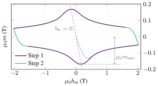
Figure 15: Reference magnetization curve for the identification of a chain of S cells.

The objective is to find the hysteresis model parameters such that $\boldsymbol{b}=\boldsymbol{\mathcal{B}}(\boldsymbol{h})$ is as close as possible to $\boldsymbol{b}_{\text{in}}$ when $\boldsymbol{h}=\boldsymbol{h}_{\text{in}}$. The proposed identification procedure is decomposed in two steps.

Step 1: Fitting the field-dependent scaling

The first step is to fit the irreversibility parameter scaling, $f_{\kappa}(\boldsymbol{b})$, introduced in Eq. (22) to account for the field-dependent critical current density. For this, we consider parts of the magnetization cycle in which the superconductor is fully magnetized. In Fig. 15, this corresponds to the purple curves labelled as Step 1.

For a chain of S cell, using Eqs. (8) and (23), the total magnetization is given by

$$\boldsymbol{m} =\boldsymbol{b}/\mu_{0}-\boldsymbol{h}=\sum_{k=1}^{N}\alpha_{k}\boldsymbol{h}_{\text{rev},k}-\boldsymbol{h}$$

$$=\sum_{k=1}^{N}\alpha_{k}\left(\boldsymbol{h}_{\text{rev},k}-\boldsymbol{h}\right)=\sum_{k=1}^{N}\alpha_{k}\boldsymbol{h}_{\text{irr},k}.$$ (40)

In the fully magnetized situation and with a unidirectional excitation, we have

$$|m|=\sum_{k=1}^{N}\alpha_{k}\kappa_{k}(\boldsymbol{b})=f_{\kappa}(\boldsymbol{b})\underbrace{\sum_{k=1}^{N}\alpha_{k}\bar{\kappa}_{k}}_{m_{\text{max}}},$$ (41)

with $m_{\text{max}}$ (in A/m) the maximum magnetization. As a result, the scaling function $f_{\kappa}(\boldsymbol{b})$ directly describes the shape of the purple curves in Fig. 15.

A simple approach consists in choosing $f_{\kappa}(\boldsymbol{b})=j_{\text{c}}(\boldsymbol{b})/j_{\text{c}}(\boldsymbol{0})$ as a scaling over the whole field range. This however does not lead to very accurate results at low fields for which $j_{\text{c}}$ strongly depends on $\boldsymbol{b}$. The reason is that the strand magnetization depends on the actual field distribution inside it, which is not uniform, and not only on the average vector $\boldsymbol{b}_{\text{in}}$. The larger the filaments in the strand, the larger the variation of $\boldsymbol{b}$ within each filament.

A better approach is to directly identify the scaling $f_{\kappa}(\boldsymbol{b})$ on the reference curve. The purple curves can therefore be used to directly define $f_{\kappa}(\boldsymbol{b})$ in the available field range. Outside of the field range, $f_{\kappa}(\boldsymbol{b})=j_{\text{c}}(\boldsymbol{b})/j_{\text{c}}(\boldsymbol{0})$ can be used as a first approximation.

In some circumstances, the maximum magnetization may not be observed at $\boldsymbol{b}_{\text{in}}=\boldsymbol{0}$ exactly. In such a case, the scaling $f_{\kappa}$ can be written in terms of a weighted sum such as $u\boldsymbol{b}+(1-u)\mu_{0}\boldsymbol{h}$, with $u\in[0,1]$ to be chosen.

Step 2: Choosing the $\bar{\kappa}_{k}$ and fitting the weights $\alpha_{k}$

The second step consists in finding the remaining parameters, $\bar{\kappa}_{k}$ and $\alpha_{k}$, in order to reproduce transition branches between fully magnetized states, such as those labelled as Step 2 in Fig. 15.

The proposed procedure consists in choosing a priori the $N$ values $\bar{\kappa}_{k}$ and then fixing the weights $\alpha_{k}$ accordingly. For simplicity, we arrange the $\bar{\kappa}_{k}$ values in increasing order with respect to $k$ and start with $\bar{\kappa}_{1}=0$ A/m.

We consider the virgin magnetization curve represented by the dotted curve in Fig. 15. Initially, $h_{\text{rev},k}=0$, $\forall k=1,\dots,N$. As the magnetic field $h_{\text{in}}$ progressively increases, it reaches the surface of the cell spheres one by one (see Fig. 8). This happens at successive threshold field values that depend on the $\bar{\kappa}_{k}$ constants and on the $f_{\kappa}(b_{\text{in}})$ scaling determined in Step 1. We denote these threshold fields as $h_{k}$.

For $h<h_{k}$, we have $h_{\text{rev},j}=0$, $\forall j=k,\dots,N$, such that only the first $k-1$ cells contribute to the magnetic flux density $b$. The weights $\alpha_{k-1}$ can therefore be successively determined by forcing the solution of the hysteresis model to match the reference solution at each $h_{k}$, for $k=2,\dots,N$. The last weight $\alpha_{N}$ is calculated so that all weights add up to one.

The choice of the number of cells $N$ and the a priori distribution of values for the $\bar{\kappa}_{k}$ depend on the sought accuracy and application. This is discussed in Section 6.

5.2 Chain of CS cells

For a chain of CS cells, there are $5N$ parameters to choose: $\alpha_{k}$, $\kappa_{k}$, $\tau_{\text{e},k}$, $\tau_{\text{c},k}$, and $\chi_{k}$, for $k=1,\dots,N$. To identify all these parameters, reference solutions at different frequencies are necessary.

A reference solution at a sufficiently low frequency for the eddy and coupling current effects to be negligible can be used exactly as described in the previous section to identify the $\alpha_{k}$ and $\kappa_{k}$ (with both the $f_{\kappa}(\boldsymbol{b})$ scaling and the $\bar{\kappa}_{k}$ values). This leads to a number of $3N$ remaining parameters.

The time constants $\tau_{\text{e},k}$ and $\tau_{\text{c},k}$ can be chosen so that the positions of the peaks in eddy and coupling losses respectively correspond to those of reference solutions, such as shown in Fig. 3. Choosing identical values for all the cells already leads to good results within limited amplitude ranges. To reproduce the observation that the maxima in coupling and eddy loss are observed at lower frequencies when the field amplitude increases, one can choose larger values of $\tau_{\text{e},k}$ and $\tau_{\text{c},k}$ for cells associated with larger irreversibility parameters $\kappa_{k}$. This will be illustrated in Section 7.

Once the time constants are chosen, the only remaining parameters are the irreversibility parameters $\chi_{k}(\boldsymbol{b})=f_{\chi}(\boldsymbol{b})\bar{\chi}_{k}$. The scaling $f_{\chi}(\boldsymbol{b})$ can be chosen as in the static case (Step 1), based on a reference solution at a sufficiently high frequency for the dynamic effects to be visible in the magnetization curve, e.g., at $f=100$ Hz for the 54-filament strand, as shown in Fig. 7. Then, the values $\bar{\chi}_{k}$ can be identified in order to best reproduce the transition branches, as in Step 2 of the static case, but now with values $\bar{\chi}_{k}$ as unknowns instead of the weights $\alpha_{k}$ which are already fixed.

6 Results with a chain of S cells

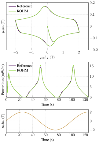
(a) Major loop $h_{\text{app}}^{(1)}(t)$.

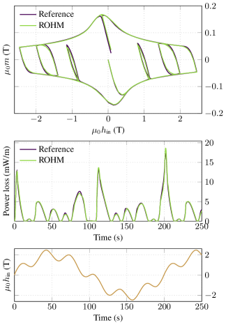
(b) Minor loops $h_{\text{app}}^{(2)}(t)$.

Figure 16: Comparison of the hysteresis model results with a reference solution. Unidirectional transverse magnetic field. Chain of S cells with $N=6$ cells, parameters of Table 2. (a) Harmonic excitation $h_{\text{app}}^{(1)}(t)$. (b) Biharmonic excitation $h_{\text{app}}^{(2)}(t)$. (Up) Magnetization loop. (Middle) Dissipated power per unit length as a function of time, equal to $a\,p_{\text{irr}}(t)$, with $a=\pi d^{2}/4$ the surface area of the strand cross section. (Down) Internal magnetic field, the input of the hysteresis model.

The first application consists in the 54-filament strand presented in Section 2, subject to a transverse field varying sufficiently slowly for the eddy and coupling current effects to be negligible, that is, with frequencies of the order of $f=0.01$ Hz. For the reference solution, we assume a non-conducting matrix and use a classical $h$-$\phi$-formulation [41], so that coupling effects are completely removed.

Because of the finite value of the power index $n=30$, the strand response is not truly rate-independent (this would only be the case at the limit $n\to\infty$). Still, we model the macroscopic strand response (magnetization and loss) with a chain of S cells as a first approximation, and show that it already provides very good results.

We start the analysis by identifying the parameters of the chain of S cells. We then compare the prediction of the resulting model for different types of excitations, both unidirectional and bidirectional.

6.1 Parameter identification

The reference solution is the major loop represented in Fig. 15. We choose $N=6$ and apply the two-step procedure described in Section 5.1 with $N$ equally spaced values $\mu_{0}\bar{\kappa}_{k}$ from $0$ T to $0.75$ T. The obtained parameters are given in Table 2.

$k$	$\alpha_{k}$	$\mu_{0}\bar{\kappa}_{k}$
	($\%$)	(mT)
$1$	$48.24$	$0$
$2$	$18.07$	$150$
$3$	$16.99$	$300$
$4$	$9.31$	$450$
$5$	$5.16$	$600$
$6$	$2.22$	$750$

Table 2: Parameters of a chain of S cells with $N=6$, identified on the reference magnetization loop shown in Fig. 15.

It is interesting to notice that the first S cell, which is anhysteretic, almost contributes to half of the magnetic flux density. This is due to the large fraction of normal conductor in the strand, the matrix, which does not behave as a hysteretic material.

6.2 Unidirectional excitation

Using the parameters obtained above, we compare the predictions of the hysteresis model in terms of magnetization and loss for two unidirectional excitations along $\hat{\boldsymbol{e}}_{y}$. The first one is a harmonic field:

$$\mu_{0}h_{\text{app}}^{(1)}(t) =\mu_{0}h_{\text{max}}\sin(2\pi ft),$$ (42)

with $\mu_{0}h_{\text{max}}=2$ T and $f=0.01$ Hz. The second one is a biharmonic field, so as to produce minor magnetization loops:

$$\mu_{0}h_{\text{app}}^{(2)}(t) =\mu_{0}h_{\text{max}}\left(\sin(\pi ft)+0.25\sin(6\pi ft)\right).$$ (43)

Results are given in Fig. 16. With $N=6$ cells, the hysteresis model is capable of reproducing faithfully both major and minor magnetization loops. The loss is accurately reproduced in both cases, with a relative error on the total loss below $1\%$.

The influence of the number of cells on the relative error on total loss is shown in Fig. 17. For the considered excitations, increasing the number of cells helps reducing the error for low $N$ values ($\leq 3$), but the error then stabilizes to a non-zero value. One source of error is related to the scaling function $f_{\kappa}(\boldsymbol{b})$ for irreversibility parameters, which is only approximate. Indeed, in reality, the magnetic flux density $\boldsymbol{b}$ is not uniform in the filament, but rather varies due to the screening currents and geometrical effects. Also, as mentioned above, the reference solution is not truly rate-independent, due to the finite $n$ value in the power law.

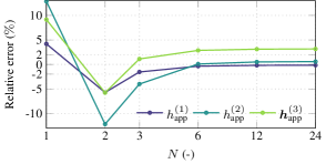
Figure 17: Evolution of the relative error $(Q_{\text{hyst}}-Q_{\text{ref}})/Q_{\text{ref}}$ between total losses predicted by the hysteresis model ($Q_{\text{hyst}}$) and the reference model ($Q_{\text{ref}}$), for different sources, as a function of the number of cells $N$, with equally spaced values $\mu_{0}\bar{\kappa}_{k}$, from $0$ T to $0.75$ T. In the case $N=1$, $\mu_{0}\bar{\kappa}_{1}=0.168$ T and $\alpha_{1}=1$.

The major advantage of the method is its computational efficiency. Once the model parameters are identified, solving the hysteresis model is tremendously faster than solving a finite element model (typically a few milliseconds compared to a few tens of minutes). This efficiency is crucial in view of homogenizing full-scale superconducting systems.

In practice, the number of cells and the distribution of $\bar{\kappa}_{k}$ values must be chosen depending on the actual excitations to be considered in the end application. A chain of S cells produces no loss for field variations smaller than the smallest non-zero irreversibility parameter $\kappa_{k}(\boldsymbol{b})$, as illustrated in Fig. 18. To reproduce accurately power loss at low fields, or for low field ripples, the chain of S cells must therefore contain cells with sufficiently small irreversibility parameters. This will be further illustrated in the case of a chain of CS cells in Section 7.

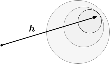
Figure 18: Illustration of a chain of S cells with $N=3$. The centers of the spheres are at positions $\boldsymbol{h}_{\text{rev},k}$, established by the history of $\boldsymbol{h}$. Variations of the magnetic field $\boldsymbol{h}$ that stay inside the smallest sphere do not produce any loss.

6.3 Bidirectional excitation

The parameters were identified based on the results of a unidirectional excitation, but all the hysteresis model equations are vectorial, and the model is therefore directly applicable to general excitations. We show in Fig. 19 the results for a bidirectional rotating transverse field excitation defined by:

$$\mu_{0}\boldsymbol{h}_{\text{app}}^{(3)}(t)=\quad \mu_{0}h_{\text{max}}\sin(\pi ft)\sin(\pi ft)\hat{\boldsymbol{e}}_{x}$$

$$+ \mu_{0}h_{\text{max}}\sin(\pi ft)\cos(\pi ft)\hat{\boldsymbol{e}}_{y},$$ (44)

with $\mu_{0}h_{\text{max}}=2$ T, $f=0.01$ Hz, and $\hat{\boldsymbol{e}}_{x}$, $\hat{\boldsymbol{e}}_{y}$ the unit vectors in $x$-, $y$-directions. The influence of the number of cells $N$ on the relative error is shown in Fig. 17, a constant error of $\approx 3\%$ remains for large values of $N$.

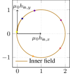
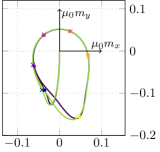
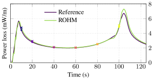
Figure 19: Comparison of hysteresis model results with a reference solution. Rotating transverse magnetic field $\boldsymbol{h}_{\text{app}}^{(3)}(t)$. Chain of S cells with $N=6$ cells and parameters of Table 2. Solutions at selected time instants are indicated by the colored circles (reference solution) and crosses (hysteresis model). (Up) Internal magnetic field and magnetization of the filament (same legend as in the bottom sub-figure). Values are in tesla (T). (Down) Dissipated power per unit length as a function of time.

The hysteresis model reproduces well the magnetization and power loss. The angle between the inner field $\boldsymbol{h}_{\text{in}}$ and the magnetization vector $\boldsymbol{m}$ is faithfully described, as shown by the solutions at selected time instants in Fig. 19. The agreement is not perfect, but very satisfying provided that the model parameters were fully identified using results from a unidirectional situation, with absolutely no information about the strand response in more general cases. We let the questions of improving the agreement and tackling anisotropic systems for further works.

7 Results with a chain of CS cells

As a generalization of the previous section, we consider the same 54-filament strand subject to a transverse field, but now with higher rates of field changes, so that both magnetization and loss exhibit frequency dependence. The reference solutions are obtained as described in Section 2 with the CATI method in order to account for coupling current effects.

We start the analysis by choosing the hysteresis model parameters based on reference solutions. We then illustrate the results for wide ranges of field amplitudes and frequencies.

7.1 Parameter identification

We choose the chain structure represented in Fig. 14. Compared to the chain of S cells of the previous section, two cells now have a zero irreversibility parameter, $\kappa_{1}=0$ A/m and $\kappa_{2}=0$ A/m. They allow to reproduce losses at low fields, for which filament loss is small with respect to coupling and eddy loss. These two cells allow to reproduce the transitions between the three regimes illustrated in Fig. 20 at low fields, associated with different magnetization slopes, as shown in Fig. 21. The curves are obtained with the parameter values of Table 3, which are discussed below.

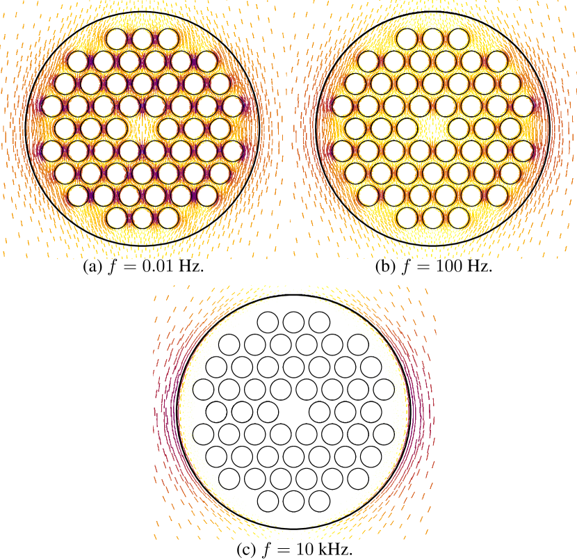
Figure 20: Field distribution at low fields ($\mu_{0}h=10$ mT here) and different frequencies. The lines are parallel to the local magnetic field, the larger and darker they are, the higher the field amplitude. (a) Uncoupled filament and limited magnetization. (b) Increased magnetization due to coupled filaments. (c) Close to perfect diamagnetism due to eddy currents.

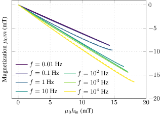
Figure 21: Strand magnetization for $\mu_{0}h_{\text{max}}=10$ mT at different frequencies, from virgin state at time $t=0$ to time $t=0.25/f$ (for better clarity). Dashed lines are reference solutions and solid lines are from the hysteresis model.

At low frequencies, the dominant contribution to magnetization and loss comes from superconducting filament hysteresis. We can reuse the material parameters found in the previous section for the chain of S cells as was given in Table 2. In order to reproduce losses at fields lower than $0.15$ T, we also introduce $8$ new cells with lower irreversibility parameters, logarithmically spaced from $1$ mT to $80$ mT. The associated weights can be identified as proposed in Section 5.1, or based on analytical solutions at low fields.

We then choose the time constants. A good fit with the reference solution is obtained with the values provided in Table 3. Larger time constants are chosen for cells associated with higher irreversibility parameters, in order to reproduce the shifts of the peak coupling and eddy loss observed in Fig. 3 and discussed in Section 2.3.

Finally, we fix the scaling $f_{\chi}(\boldsymbol{b})$ and the parameters $\bar{\chi}_{k}$. We found that a decent fit is obtained with

$$f_{\chi}(\boldsymbol{b})=\frac{1-\|\boldsymbol{b}\|/b_{0}}{1+\|\boldsymbol{b}\|/b_{1}},$$ (45)

with $b_{0}=15$ T and $b_{1}=4$ T. The parameters $\bar{\chi}_{k}$ are then tuned manually to obtain the values in Table 3.

$k$	$\alpha_{k}$	$\mu_{0}\bar{\kappa}_{k}$	$\tau_{\text{e},k}$	$\tau_{\text{c},k}$	$\mu_{0}\bar{\chi}_{k}$
(-)	($\%$)	(mT)	(ms)	(s)	(T)
$1$	$16.38$	$0.0$	$0.02$	$0.00$	$0.00$
$2$	$22.62$	$0.0$	$0.02$	$0.08$	$1.13$
$3$	$0.05$	$1.0$	$0.02$	$0.08$	$0.01$
$4$	$0.10$	$1.9$	$0.02$	$0.08$	$0.02$
$5$	$0.19$	$3.5$	$0.02$	$0.08$	$0.03$
$6$	$0.35$	$6.5$	$0.02$	$0.08$	$0.07$
$7$	$0.66$	$12.2$	$0.02$	$0.08$	$0.09$
$8$	$1.24$	$22.9$	$0.02$	$0.08$	$0.14$
$9$	$2.32$	$42.9$	$0.02$	$0.08$	$0.21$
$10$	$4.33$	$80.2$	$0.02$	$0.08$	$0.40$
$11$	$18.07$	$150.0$	$0.30$	$0.28$	$1.50$
$12$	$16.99$	$300.0$	$0.30$	$0.28$	$2.10$
$13$	$9.31$	$450.0$	$0.30$	$0.28$	$3.15$
$14$	$5.16$	$600.0$	$0.30$	$0.28$	$4.20$
$15$	$2.22$	$750.0$	$0.30$	$0.28$	$5.25$

Table 3: Parameters of a chain of CS cells with $N=15$.

7.2 Results and numerical performance

Using the model parameters given in Table 3, we compare the predictions of the hysteresis model with the reference solutions. The power loss per cycle as a function of frequency and selected magnetization loops are given in Figs. 22 and 23. The power loss per cycle is also presented as a map in Fig. 24, by interpolating the results of $400$ simulations, spanning over $25$ frequencies and $16$ field amplitudes, logarithmically spaced.

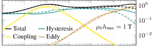
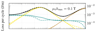
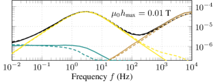
Figure 22: Power loss per cycle for three different field amplitudes as a function of frequency. Solid curves are results from the hysteresis model with parameters of Table 3 and dashed curves are reference solutions. The legend is the same for the three subfigures.

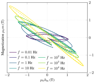
Figure 23: Strand magnetization for $\mu_{0}h_{\text{max}}=1$ T at different frequencies. Solid curves are results from the hysteresis model with parameters of Table 3 and dashed curves are reference solutions.

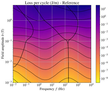
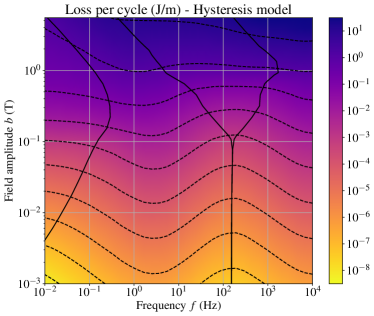
Figure 24: Total loss per cycle and per unit length as a function of the frequency and amplitude of the applied field. Dashed curves are contour lines of equal loss. Solid curves delimit areas of distinct dominant loss contributions (from left to right: hysteresis in uncoupled filaments, coupling loss, hysteresis in coupled filaments, and eddy losses). (Left) Reference model, adapted from [31]. (Right) Prediction of the hysteresis model with the parameters given in Table 3.

The overall agreement on the total loss and magnetization is very good. The hysteresis model correctly reproduces the different regimes of distinct dominant loss contributions and describes the magnetization faithfully. The difference with the reference solution is higher at high frequency and high fields, as can be seen on the contour lines in the top right corners in Fig. 24. This can be improved with a careful choice of model parameters, but as discussed in Section 3.3, the matching will never be perfect in the limit $f\to\infty$ as the CS cells do not reproduce a $1/\sqrt{f}$ decrease of the loss per cycle, but rather a $1/f$ decrease. For not too high frequencies however, the importance of this effect is limited.

The major advantage of the hysteresis model compared to the detailed simulations is the very small associated computational work. Even with $N=15$ cells, the whole loss map on the right of Fig. 24, which consists of $400$ hysteresis model simulations, can be performed in a few seconds, whereas the reference model requires $26$ days of computation time in total to generate the loss map on the left of Fig. 24.

As described in Section 4.4, the hysteresis model can also easily be included in a FE model as a homogenized material property for the local fields $\boldsymbol{h}$ and $\boldsymbol{b}=\boldsymbol{\mathcal{B}}(\boldsymbol{h})$. An illustration of the obtained field is given in Fig. 25 in the simple case of a single strand surrounded by air, obtained with the $\phi$-formulation. The hysteresis model reproduces the magnetization of the detailed strand model, such that the field seen outside of it is identical to that seen outside of the detailed strand.

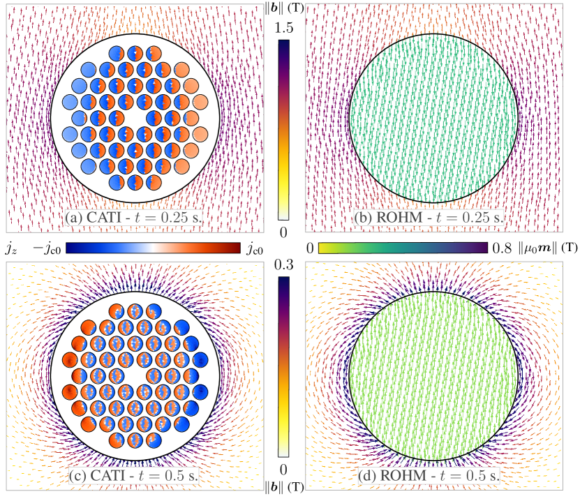
Figure 25: Solutions of the reference CATI model and the ROHM model for $\mu_{0}h_{\text{max}}=1$ T and $f=1$ Hz. (a-b) Solutions at $t=0.25$ s. (c-d) Solutions at $t=0.5$ s. Arrows outside of the strand represent the magnetic flux density $\boldsymbol{b}$ (shared color scale in the middle). Colored elements in (a) and (c) represent the $z$-component of the current density $\boldsymbol{j}$ (color scale on the left, with $j_{\text{c0}}=3\times 10^{10}$ A/m²). Arrows inside the strand in (b) and (d) represent the magnetization $\mu_{0}\boldsymbol{m}=\boldsymbol{b}-\mu_{0}\boldsymbol{h}$ (color scale on the right).

In superconducting magnets, many strands are combined together into cables, which themselves are wound around the magnet aperture. The hysteresis model can be used to homogenize the large number of strands into an equivalent homogeneous material. In such a case, which is let for further work, the reference detailed solution should be that of a close-packed set of strands, which can typically be modelled via appropriate periodic boundary conditions [14], rather than a single strand in air, as was done here for the sake of illustration. This may result in different model parameters, but the general approach is unchanged.

8 Conclusion

In this work, we introduced the Reduced Order Hysteretic Magnetization (ROHM) model to represent the magnetization and instantaneous loss in composite superconductors subject to transient external fields. This model is designed by adapting to superconducting systems the state-of-the-art energy-based model developed in the context of ferromagnetic hysteresis [27]. We focused specifically on the case of a multifilamentary superconducting strand and proposed two models: a rate-independent model, describing hysteresis in superconducting filaments, and a rate-dependent model, accounting for filament coupling, coupling current, and eddy current effects.

We proposed a parameter identification approach for both models and described their inclusion in a finite element framework. Finally, we demonstrated that these models help to strongly reduce the computational cost compared to conventional simulations, while offering a very good accuracy in a wide range of field amplitudes and rates of field change.

This work constitutes a first step towards the homogenization of superconducting magnets, in which the large number of turns makes detailed simulations unrealistically expensive. Replacing the coil windings by homogenized material properties such as the proposed ROHM model allows to describe magnetization and loss efficiently. Further work is necessary to include non-zero transport current, which was not covered in this paper.

Extension of the method to anisotropic systems such as high-temperature superconducting tapes or stacks of tapes in view of their homogenization can also be considered as further work.

Appendix A Magnetization in 2D Problems

In this section, we justify the introduction of a factor $2$ in the magnetization Eq. (1), in the case of an infinitely long problem solved in 2D with perpendicular currents.

The magnetic dipole moment $\boldsymbol{M}$ of a current density distribution $\boldsymbol{j}$ in a given volume $V$ is evaluated as

$$\boldsymbol{M}=\frac{1}{2}\int_{V}\boldsymbol{x}\times\boldsymbol{j}\,\text{d}V,$$ (46)

with $\boldsymbol{x}$ the position vector. Consider a rectangular current tube of cross section $\text{d}S$, width $w$, and length $l$, carrying a current $\text{d}I=\boldsymbol{j}\cdot\text{d}\boldsymbol{S}$, as illustrated in Fig. 26. Accounting for the four sides of the rectangle, the contribution of this current loop to the total magnetic dipole moment is $wl\,\text{d}I$. Long and short sides of the rectangle contribute equally to the total magnetic dipole moment.

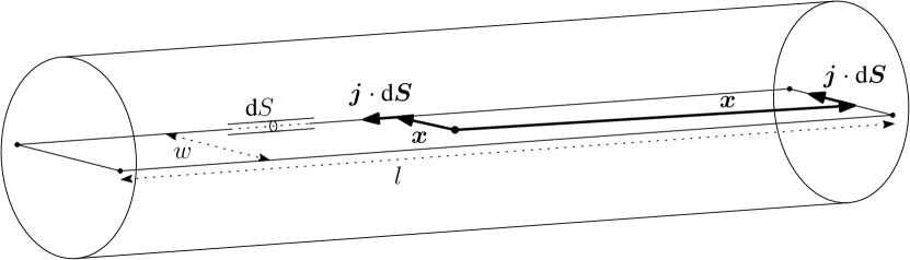
Figure 26: Magnetic dipole moment of a current tube in a cylinder.

When the geometry is sufficiently long for end effects to be neglected, the problem is usually solved in 2D and per unit length, on a cross section of the conducting cylinder. In such a case, however, one must still account for the fact that all current loops close at the end of the cylinder, i.e., at infinity, for computing the magnetization per unit length. These closing currents are not part of the 2D solution, and are then missing from any magnetization calculation performed solely on the 2D cross section. Because the closing currents contribute to exactly half of the magnetic dipole moment, one can account for them by introducing a factor $2$, as is done in Eq. (1).

Appendix B Applied Field and Internal Field

The power loss per cycle $Q_{\text{tot}}$ given by Eq. (4) can equivalently be computed in terms of $\boldsymbol{h}_{\text{in}}=\boldsymbol{h}_{\text{app}}-\boldsymbol{m}/2$. Indeed, as also shown in [38],

$$Q_{\text{tot}} =a\oint\mu_{0}\boldsymbol{h}_{\text{app}}\cdot\text{d}\boldsymbol{m}$$

$$=a\oint\mu_{0}(\boldsymbol{h}_{\text{in}}+\boldsymbol{m}/2)\cdot\text{d}\boldsymbol{m}$$

$$=a\oint\mu_{0}\boldsymbol{h}_{\text{in}}\cdot\text{d}\boldsymbol{m}+\frac{a\mu_{0}}{2}\underbrace{\oint\boldsymbol{m}\cdot\text{d}\boldsymbol{m}}_{=0\text{ if closed}}$$

$$=a\oint\mu_{0}\boldsymbol{h}_{\text{in}}\cdot\text{d}\boldsymbol{m}.$$ (47)

That is, the areas enclosed by the loops represented in Figs. 5 and 7 are identical.

Appendix C Hysteresis Model Jacobian

The inclusion of a hysteresis model into a FE model makes the problem nonlinear. Equations must then be solved iteratively. In order to implement the efficient Newton-Raphson iterative technique, the Jacobian of the hysteresis law $\boldsymbol{b}=\boldsymbol{\mathcal{B}}(\boldsymbol{h})$ must be evaluated. It is a tensor of order two which reads as follows, using Eq. (23):

$$\frac{\partial\boldsymbol{b}}{\partial\boldsymbol{h}}=\sum_{k=1}^{N}\alpha_{k}\mu_{0}\frac{\partial\boldsymbol{h}_{\text{rev},k}}{\partial\boldsymbol{h}}.$$ (48)

Its expression can be computed independently for each cell. Below, we give its expression for the simple case of a S cell and then generalize for a CS cell. We drop the index $k$ for conciseness.

C.1 S cell

For a S cell, the reversible field $\boldsymbol{h}_{\text{rev}}$ is updated with Eq. (4.1). The derivative of this update rule is given by

$$\frac{\partial\boldsymbol{h}_{\text{rev}}}{\partial\boldsymbol{h}} =\left\{\begin{aligned} &\mathbf{0},\quad\text{if }\|\boldsymbol{h}-\boldsymbol{h}_{\text{rev(p)}}\|\leq\kappa,\\ &\left(1-\frac{\kappa}{\|\boldsymbol{h}-\boldsymbol{h}_{\text{rev(p)}}\|}\right)\mathbf{I}+\frac{\kappa}{\|\boldsymbol{h}-\boldsymbol{h}_{\text{rev(p)}}\|^{3}}\mathbf{K},\\ &\qquad\text{otherwise,}\end{aligned}\right.$$

$$=\boldsymbol{\mathcal{W}}_{\kappa}(\boldsymbol{h},\boldsymbol{h}_{\text{rev(p)}}),$$ (49)

with $\mathbf{I}$ the second-order identity tensor and $\mathbf{K}$ defined by the following dyadic product:

$$\mathbf{K}=(\boldsymbol{h}-\boldsymbol{h}_{\text{rev(p)}})\otimes(\boldsymbol{h}-\boldsymbol{h}_{\text{rev(p)}}).$$ (50)

C.2 CS cell

For a CS cell, we first compute $\boldsymbol{h}_{\text{coupling}}^{\text{trial}}$ using Eq. (30). In the case $\|\boldsymbol{h}_{\text{coupling}}^{\text{trial}}\|\leq\chi$, using Eqs. (35), (31), and (32), we have the reversible field given by

$$\boldsymbol{h}_{\text{rev}}=\frac{\Delta t}{\Delta t+\tau_{\text{e}}+\tau_{\text{c}}}\left(\boldsymbol{g}+\frac{\tau_{\text{e}}+\tau_{\text{c}}}{\Delta t}\boldsymbol{h}_{\text{rev(p)}}\right)$$ (51)

whose derivative reads

$$\frac{\partial\boldsymbol{h}_{\text{rev}}}{\partial\boldsymbol{h}} =\frac{\Delta t}{\Delta t+\tau_{\text{e}}+\tau_{\text{c}}}\frac{\partial\boldsymbol{g}}{\partial\boldsymbol{h}}$$

$$=\frac{\Delta t}{\Delta t+\tau_{\text{e}}+\tau_{\text{c}}}\boldsymbol{\mathcal{W}}_{\kappa}(\boldsymbol{h},\boldsymbol{g}_{\text{(p)}}),$$ (52)

where $\boldsymbol{\mathcal{W}}_{\kappa}$ is the second-order tensor defined in Eq. (C.1), written here as a function of $\boldsymbol{g}_{\text{(p)}}$ instead of $\boldsymbol{h}_{\text{rev(p)}}$.

By contrast, if $\|\boldsymbol{h}_{\text{coupling}}^{\text{trial}}\|>\chi$, one must use Eqs. (35), (33), and (34), which yields the following reversible field

$$\boldsymbol{h}_{\text{rev}}=\frac{\Delta t}{\Delta t+\tau_{\text{e}}}\left(\boldsymbol{g}-\chi\frac{\boldsymbol{g}-\boldsymbol{h}_{\text{rev(p)}}}{\|\boldsymbol{g}-\boldsymbol{h}_{\text{rev(p)}}\|}+\frac{\tau_{\text{e}}}{\Delta t}\boldsymbol{h}_{\text{rev(p)}}\right)$$ (53)

whose derivative reads

$$\frac{\partial\boldsymbol{h}_{\text{rev}}}{\partial\boldsymbol{h}} =\frac{\Delta t}{\Delta t+\tau_{\text{e}}}\left(\frac{\partial\boldsymbol{g}}{\partial\boldsymbol{h}}-\frac{\partial}{\partial\boldsymbol{g}}\left(\chi\frac{\boldsymbol{g}-\boldsymbol{h}_{\text{rev(p)}}}{\|\boldsymbol{g}-\boldsymbol{h}_{\text{rev(p)}}\|}\right)\cdot\frac{\partial\boldsymbol{g}}{\partial\boldsymbol{h}}\right)$$

$$=\frac{\Delta t}{\Delta t+\tau_{\text{e}}}\boldsymbol{\mathcal{W}}_{\chi}(\boldsymbol{g},\boldsymbol{h}_{\text{rev(p)}})\cdot\boldsymbol{\mathcal{W}}_{\kappa}(\boldsymbol{h},\boldsymbol{g}_{\text{(p)}}),$$ (54)

where $\boldsymbol{\mathcal{W}}_{\chi}$ is the second-order tensor defined by

$$\boldsymbol{\mathcal{W}}_{\chi}(\boldsymbol{g},\boldsymbol{h}_{\text{rev(p)}})=\left(1-\frac{\chi}{\|\boldsymbol{g}-\boldsymbol{h}_{\text{rev(p)}}\|}\right)\mathbf{I}$$

$$+\frac{\chi}{\|\boldsymbol{g}-\boldsymbol{h}_{\text{rev(p)}}\|^{3}}\mathbf{L},$$ (55)

with

$$\mathbf{L}=(\boldsymbol{g}-\boldsymbol{h}_{\text{rev(p)}})\otimes(\boldsymbol{g}-\boldsymbol{h}_{\text{rev(p)}}).$$ (56)

References

References

- [1] C. P. Bean, “Magnetization of hard superconductors,” Physical review letters, vol. 8, no. 6, p. 250, 1962.
- [2] C. P. Bean, “Magnetization of high-field superconductors,” Reviews of modern physics, vol. 36, no. 1, p. 31, 1964.
- [3] E. H. Brandt, “Flux line lattice in high-Tc superconductors: anisotropy, elasticity, fluctuation, thermal depinning, AC penetration and susceptibility,” Physica C: Superconductivity, vol. 195, no. 1-2, pp. 1–27, 1992.
- [4] R. Richardson, O. Pla, and F. Nori, “Confirmation of the modified Bean model from simulations of superconducting vortices,” Physical review letters, vol. 72, no. 8, p. 1268, 1994.
- [5] A. Campbell, “A general treatment of losses in multifilamentary superconductors,” Cryogenics, vol. 22, no. 1, pp. 3–16, 1982.
- [6] M. N. Wilson, “Superconducting magnets,” Clarendon Press, United Kingdom, 1983.
- [7] A. P. Verweij, “Electrodynamics of superconducting cables in accelerator magnets.,” PhD thesis, Twente University, Enschede, 1997.
- [8] M. Aleksa, B. Auchmann, S. Russenschuck, and C. Vollinger, “A vector hysteresis model for superconducting filament magnetization in accelerator magnets,” IEEE Transactions on Magnetics, vol. 40, no. 2, pp. 864–867, 2004.
- [9] J. Rhyner, “Magnetic properties and AC-losses of superconductors with power law current—voltage characteristics,” Physica C: Superconductivity, vol. 212, no. 3-4, pp. 292–300, 1993.
- [10] B. Shen, F. Grilli, and T. Coombs, “Review of the AC loss computation for HTS using H formulation,” Superconductor Science and Technology, vol. 33, no. 3, p. 033002, 2020.
- [11] N. Riva, A. Halbach, M. Lyly, C. Messe, J. Ruuskanen, and V. Lahtinen, “H-phi formulation in Sparselizard combined with domain decomposition methods for modeling superconducting tapes, stacks, and twisted wires,” IEEE Transactions on Applied Superconductivity, vol. 33, no. 5, pp. 1–5, 2023.
- [12] A. Marteau, I. Niyonzima, G. Meunier, J. Ruuskanen, N. Galopin, P. Rasilo, and O. Chadebec, “Magnetic field upscaling and B-conforming magnetoquasistatic multiscale formulation,” IEEE Transactions on Magnetics, 2023.
- [13] M. El Feddi, Z. Ren, A. Razek, and A. Bossavit, “Homogenization technique for maxwell equations in periodic structures,” IEEE Transactions on magnetics, vol. 33, no. 2, pp. 1382–1385, 1997.
- [14] G. Meunier, V. Charmoille, C. Guérin, P. Labie, and Y. Maréchal, “Homogenization for periodical electromagnetic structure: Which formulation?,” IEEE transactions on magnetics, vol. 46, no. 8, pp. 3409–3412, 2010.
- [15] J. Gyselinck, R. Sabariego, and P. Dular, “A nonlinear time-domain homogenization technique for laminated iron cores in three-dimensional finite-element models,” IEEE transactions on magnetics, vol. 42, no. 4, pp. 763–766, 2006.
- [16] J. Gyselinck and P. Dular, “Frequency-domain homogenization of bundles of wires in 2-D magnetodynamic FE calculations,” IEEE transactions on magnetics, vol. 41, no. 5, pp. 1416–1419, 2005.
- [17] R. V. Sabariego, P. Dular, and J. Gyselinck, “Time-domain homogenization of windings in 3-D finite element models,” IEEE transactions on magnetics, vol. 44, no. 6, pp. 1302–1305, 2008.
- [18] C. Völlinger, Superconductor magnetization modeling for the numerical calculation of field errors in accelerator magnets. PhD thesis, Berlin, Tech. U., 2002.
- [19] F. Preisach, “Über die magnetische nachwirkung,” Zeitschrift für physik, vol. 94, no. 5, pp. 277–302, 1935.
- [20] M. Sjöström, Hysteresis modelling of high temperature superconductors. PhD thesis, EPFL, 2001.
- [21] M. Sjöström, B. Dutoit, and J. Duron, “Equivalent circuit model for superconductors,” IEEE transactions on applied superconductivity, vol. 13, no. 2, pp. 1890–1893, 2003.
- [22] A. Badía and C. López, “Vector magnetic hysteresis of hard superconductors,” Physical Review B, vol. 65, no. 10, p. 104514, 2002.
- [23] D. C. Jiles and D. L. Atherton, “Theory of ferromagnetic hysteresis,” Journal of magnetism and magnetic materials, vol. 61, no. 1-2, pp. 48–60, 1986.
- [24] L. Chua and K. Stromsmoe, “Lumped-circuit models for nonlinear inductors exhibiting hysteresis loops,” IEEE Transactions on Circuit Theory, vol. 17, no. 4, pp. 564–574, 1970.
- [25] L. Chua and S. Bass, “A generalized hysteresis model,” IEEE Transactions on Circuit Theory, vol. 19, no. 1, pp. 36–48, 1972.
- [26] A. Bergqvist, “Magnetic vector hysteresis model with dry friction-like pinning,” Physica B: Condensed Matter, vol. 233, no. 4, pp. 342–347, 1997.
- [27] F. Henrotte, A. Nicolet, and K. Hameyer, “An energy-based vector hysteresis model for ferromagnetic materials,” COMPEL-The international journal for computation and mathematics in electrical and electronic engineering, vol. 25, no. 1, pp. 71–80, 2006.
- [28] F. Henrotte and K. Hameyer, “A dynamical vector hysteresis model based on an energy approach,” IEEE Transactions on Magnetics, vol. 42, no. 4, pp. 899–902, 2006.
- [29] K. Jacques, Energy-Based Magnetic Hysteresis Models-Theoretical Development and Finite Element Formulations. PhD thesis, University of Liège, 2018.
- [30] G. Zachou, M. Wozniak, E. Schnaubelt, T. Mulder, J. Dular, E. Ravaioli, and A. Verweij, “A unified common source for material properties across simulation modelling tools,” https://cern.ch/smali, 2024.
- [31] J. Dular, F. Magnus, E. Schnaubelt, A. Verweij, and M. Wozniak, “Coupled axial and transverse currents method for finite element modelling of periodic superconductors,” Superconductor Science and Technology, vol. 37, no. 9, pp. 1–18, 2024.
- [32] P. Dular, C. Geuzaine, F. Henrotte, and W. Legros, “A general environment for the treatment of discrete problems and its application to the finite element method,” IEEE Transactions on Magnetics, vol. 34, no. 5, pp. 3395–3398, 1998.
- [33] A. Vitrano, M. Wozniak, E. Schnaubelt, T. Mulder, E. Ravaioli, and A. Verweij, “An open-source finite element quench simulation tool for superconducting magnets,” IEEE Transactions on Applied Superconductivity, vol. 33, no. 5, pp. 1–6, 2023.
- [34] L. Bortot, B. Auchmann, I. C. Garcia, A. F. Navarro, M. Maciejewski, M. Mentink, M. Prioli, E. Ravaioli, S. Schoeps, and A. Verweij, “STEAM: A hierarchical cosimulation framework for superconducting accelerator magnet circuits,” IEEE Transactions on Applied Superconductivity, vol. 28, no. 3, pp. 1–6, 2017.
- [35] C. Geuzaine and J.-F. Remacle, “Gmsh: A 3D finite element mesh generator with built-in pre-and post-processing facilities,” International journal for numerical methods in engineering, vol. 79, no. 11, pp. 1309–1331, 2009.
- [36] D. J. Griffiths, Introduction to electrodynamics. Cambridge University Press, 2023.
- [37] A. Bossavit, “Remarks about hysteresis in superconductivity modelling,” Physica B: Condensed Matter, vol. 275, no. 1-3, pp. 142–149, 2000.
- [38] R. B. Goldfarb, “Internal fields in magnetic materials and superconductors,” Cryogenics, vol. 26, no. 11, pp. 621–622, 1986.
- [39] G. Morgan, “Theoretical behavior of twisted multicore superconducting wire in a time-varying uniform magnetic field,” Journal of Applied Physics, vol. 41, no. 9, pp. 3673–3679, 1970.
- [40] M. N. Wilson, “NbTi superconductors with low AC loss: A review,” Cryogenics, vol. 48, no. 7-8, pp. 381–395, 2008.
- [41] A. Bossavit, Computational electromagnetism: variational formulations, complementarity, edge elements. Academic Press, 1998.
- [42] J. Dular, C. Geuzaine, and B. Vanderheyden, “Finite-element formulations for systems with high-temperature superconductors,” IEEE Transactions on Applied Superconductivity, vol. 30, no. 3, pp. 1–13, 2019.