Qualitative Analysis and Adaptive Boosted DCA for Generalized Multi-Source Weber Problems

Abstract

This paper has two primary objectives. First, we investigate fundamental qualitative properties of the generalized multi-source Weber problem formulated using the Minkowski gauge function. This includes proving the existence of global optimal solutions, demonstrating the compactness of the solution set, and establishing optimality conditions for these solutions. Second, we apply Nesterov’s smoothing and the adaptive Boosted Difference of Convex functions Algorithm (BDCA) to solve both the unconstrained and constrained versions of the generalized multi-source Weber problems. These algorithms build upon the work presented in [6, 19]. We conduct a comprehensive evaluation of the adaptive BDCA, comparing its performance to the method proposed in [19], and provide insights into its efficiency. 
Keywords: Generalized multi-source Weber problem, Nesterov’s smoothing, DCA, boosted DCA.

1 Introduction

The single-source Weber problem (SWP), also known as the Fermat-Weber problem, is an important topic in convex optimization. It involves determining the optimal location of a source (or facility) that minimizes the sum of Euclidean distances to multiple demand points in a finite-dimensional Euclidean space. The SWP has been extensively studied in the field of facility location and is a generalization of the classical Fermat-Torricelli problem, which involves only three demand points; see, e.g., [16, 13, 18, 20] and the references therein. However, in practical applications, it is often necessary to find multiple sources to serve a finite number of demand points, leading to what are known as the multi-source Weber problem. This problem involves determining the optimal locations of a finite number of facilities to serve the demand points by minimizing the sum of the total distances from the sources to the associated demand points. In the existing literature, the multi-source Weber problems are often modeled as nonconvex nonsmooth optimization problems, which present challenges for traditional optimization techniques.

It has been shown the multi-source Weber problem belongs to the class of DC programming; see [8, 19]. Consequently, optimization techniques and algorithms from DC programming can be employed to investigate the problem from both theoretical and numerical perspectives. One of the most successful algorithms in DC programming, known as the Difference of Convex functions Algorithm (DCA), was initially introduced in [25] and further developed in [1, 24, 23, 2]. The DCA has proven to be robust and efficient across various applications, including the multi-source Weber problem (see, e.g., [24, 3, 19]). By integrating a line search technique into the DCA, a new algorithm called the Boosted Difference of Convex functions Algorithm (BDCA) was introduced in [5, 4]. This line search technique not only accelerates the convergence of the algorithm but also enables it to escape stationary points and reach a global optimal solution in many circumstances. The BDCA has been experimentally shown to outperform the DCA in many practical applications, such as the minimum sum of squares clustering and the multidimensional scaling problem; see [6].

Inspired by recent advances in DC programming and its applications, this paper explores a general model of the multi-source Weber problem using the Minkowski gauge function. Our objective is to conduct a thorough investigation of the problem’s fundamental qualitative properties and to develop effective numerical optimization methods. We begin by proving the existence of global optimal solutions, demonstrating the compactness of the solution set, and establishing optimality conditions for the problem. Next, we apply Nesterov’s smoothing technique to reduce the nonsmoothness, thereby creating a new approximate objective function that is favorable for the BDCA. Numerical experiments confirm that the BDCA is highly effective when applied to the generalized multi-source Weber problem. This approach is new, as the BDCA has not yet been applied to this general model of the multi-source Weber problem. Furthermore, we employ the penalty method to address the constrained version of the problem.

The structure of the paper is organized as follows. Section 2 introduces basic notations and definitions used throughout the paper. Section 3 establishes a global solution existence theorem for the generalized multi-source Weber problem and discusses the properties of the global solution set in detail. This section also characterizes local optimal solutions. Section 4 utilizes the algorithm from [6] to solve the generalized multi-source Weber problem for both the unconstrained and constrained cases. Section 5 focuses on enhancing the algorithms presented in the previous section and provides several examples comparing the performance of our new algorithms with that of the difference of convex algorithm. Finally, Section 6 summarizes the paper’s findings and outlines potential directions for future research.

2 Preliminaries

Throughout this paper, the Euclidean space $\mathbb{R}^{n}$, where $n\in\mathbb{N}$, is equipped with the inner product $\langle x,y\rangle=\sum_{i=1}^{n}x_{i}y_{i}$ and the norm $\|x\|=(\sum_{i=1}^{n}x_{i}^{2})^{1/2}$, where $x=(x_{1},\ldots,x_{n})$ and $y=(y_{1},\ldots,y_{n})$. However, in Section 5, we use $\|\cdot\|_{2}$ to denote the Euclidean norm, ensuring consistency with the Taxicab norm and the maximum norm, which are denoted by $\|\cdot\|_{1}$ and $\|\cdot\|_{\infty}$, respectively. The closed Euclidean ball with center $a\in\mathbb{R}^{n}$ and radius $r\geq 0$ is denoted by $\mathbb{B}[a,r]$.

Let us first recall basic notions used in the paper. The readers are referred to [1, 12, 17, 22] and the references therein for more details.

Definition 2.1.

Let $f\colon\mathbb{R}^{n}\to(-\infty,\infty]$ be a convex function. An element $v\in\mathbb{R}^{n}$ is called a subgradient of $f$ at $\bar{x}\in\mbox{\rm dom}(f)=\{x\in\mathbb{R}^{n}\;|\;f(x)<\infty\}$ if

$$\langle v,x-\bar{x}\rangle\leq f(x)-f(\bar{x})\;\mbox{\rm for all }x\in\mathbb{R}^{n}.$$

The set of all such elements $v$ is called the subdifferential of $f$ at $\bar{x}$ and is denoted by $\partial f(\bar{x})$. If $\bar{x}\not\in\mbox{\rm dom}(f)$, we set $\partial f(\bar{x})=\emptyset$.

Definition 2.2.

Let $\Omega$ be a nonempty subset of $\mathbb{R}^{n}$. The distance function associated with $\Omega$ is defined by

$$d(x;\Omega)=\inf\left\{\|x-w\|\;\big{|}\;w\in\Omega\right\},\;x\in\mathbb{R}^{n}.$$

Definition 2.3.

Let $F$ be a nonempty compact convex subset of $\mathbb{R}^{n}$ with  $0\in\mbox{\rm int}(F)$. The Minkowski function associated with $F$ is defined by

$$\rho_{F}(x)=\inf\{t\geq 0\;|\;x\in tF\},\;x\in\mathbb{R}^{n}.$$ (1)

The polar set $F^{\circ}$ of $F$ is the set

$$F^{\circ}=\{v\in\mathbb{R}^{n}\mid\langle v,x\rangle\leq 1,\;\forall x\in F\}.$$

We set $\|F\|=\sup\{\|x\|\mid x\in F\}\text{ and }\|F^{\circ}\|=\sup\{\|v\|\mid v\in F^{\circ}\}.$

Given a finite set of demand points $A=\{a^{1},\ldots,a^{m}\}\subset\mathbb{R}^{n}$, the generalized multi-source Weber problem (GMWP) can be formulated as

$$\min\left\{f_{F}(x)=\sum_{i=1}^{m}\left(\min\limits_{\ell=1,\ldots,k}\rho_{F}\left(x^{\ell}-a^{i}\right)\right)\Big{|}\;x=(x^{1},\ldots,x^{k})\in\left(\mathbb{R}^{n}\right)^{k}\right\}.$$ (2)

We always assume that

$$m\geq 2\textrm{ and }1\leq k\leq m.$$ (3)

We also assume that $F$ is a nonempty compact convex set such that $0\in\mbox{\rm int}(F)$.

Note that when $F$ is the closed unit ball in $\mathbb{R}^{n}$, problem (2) simplifies to the multi-source Weber problem (MWP), which has been recently studied in [8, 9, 10].

It can be shown that the GMWP belongs to the class of DC programming. Consider the DC program:

$$\min\left\{f(x)=g(x)-h(x)\mid x\in\mathbb{R}^{n}\right\}, \mathcal{P}$$ ()

where $g\colon\mathbb{R}^{n}\to(-\infty,\infty]$ and $h\colon\mathbb{R}^{n}\to\mathbb{R}$ are convex functions. The function $f$ defined in ($\mathcal{P}$) is called a DC function and $g-h$ is a DC decomposition of $f$. Recall that the Fenchel conjugate of $g$ is defined by

$$g^{*}(y)=\sup\{\langle y,x\rangle-g(x)\mid x\in\mathbb{R}^{n}\},\;y\in\mathbb{R}^{n}.$$

Next, we present the Difference of Convex functions Algorithm (DCA) (see [25, 24, 23]):

Algorithm 1 DCA for solving ($\mathcal{P}$)

DCA  $x_{0}\in\mbox{\rm dom}\,g,N\in\mathbb{N}$$p=0,\dots,N$

Find $y_{p}\in\partial h(x_{p})$

Find $x_{p+1}\in\partial g^{*}(y_{p})$

$x_{N+1}$

The boosted DCA (BDCA) (see [5, 6]) is an improvement of the DCA by adding a line search step incorporating an Armijo-type condition. The BDCA can be summarized below:

Algorithm 2 BDCA for solving ($\mathcal{P}$)

BDCA $x_{0}\in\mbox{\rm dom}g$, $\alpha>0$, $\beta\in(0,1)$, $N\in\mathbb{N}$$p=0,\dots,N$

Step 1: Find $y_{p}\in\partial h(x_{p})$.

Find $z_{p}\in\partial g^{*}(y_{p})$ or find $z_{p}$ approximately by solving the problem

$$\underset{x\,\in\,\mathbb{R}^{nk}}{\operatorname{min}}\;\varphi_{p}(x)=g(x)-\langle y_{p},x\rangle.$$

Step 2: Set $d_{p}=z_{p}-x_{p}$. If $d_{p}=0$ then Stop. Otherwise, go to Step 3.

Step 3: Choose any $\overline{\lambda}_{p}\geq 0$, set $\lambda_{p}=\overline{\lambda}_{p}$ $f(z_{p}+\lambda_{p}d_{p})>f(z_{p})-\alpha\lambda_{p}^{2}\|d_{p}\|^{2}$

$\lambda_{p}=\beta\lambda_{p}$

Step 4: Set $x_{p+1}=z_{p}+\lambda_{p}d_{p}$. If $x_{p+1}=x_{p}$ then Stop.

$x_{N+1}$

An advantage of BDCA over DCA is its ability to escape from stationary points and reach to the optimal solution in many circumstances. Numerical examples also shows the improvements in computational speed. BDCA has proven its effectiveness in the case where both $g$ and $h$ are differentiable in [5], and when $g$ is differentiable but $h$ is not differentiable in [6]. The problems in the our paper fall under the latter case. The readers are referred to [25, 5, 24, 23, 6] for more details.

In our paper we will use the adaptive BDCA (aBDCA), in which the self-adaptive step size strategy from [6] replaces Step 3 of the BDCA in algorithm 2. This self-adaptive strategy is detailed in algorithm 3, and allows the trial step sizes to increase or decrease depending on previous iterations.

Algorithm 3 Self-adaptive trial step size

Self-Adaptive $\lambda$$\gamma>1$, iteration $p$$p<2$

Choose some $\overline{\lambda}_{p}>0$

Obtain $\lambda_{p-2},\;\lambda_{p-1}$ from Step 3 of BDCA, algorithm 2, and $\overline{\lambda}_{p-2},\;\overline{\lambda}_{p-1}$ from previous iterations $\lambda_{p-2}=\overline{\lambda}_{p-2}$ and $\lambda_{p-1}=\overline{\lambda}_{p-1}$

$\overline{\lambda}_{p}=\gamma\lambda_{p-1}$

$\overline{\lambda}_{p}=\lambda_{p-1}$ $\overline{\lambda}_{p}$

3 Properties of Optimal Solutions to the Generalized Multi-source Weber Problem

In this section, we conduct a comprehensive study of the properties of global and local optimal solutions to the GMWP (2), extending the related existing results in [8, 19] and the references therein.

3.1 Global Optimal Solutions

We first establish the existence of global optimal solutions to the GMWP. To proceed, we present the following known results involving the Minkowski function.

Lemma 3.1.

(See [14, Lemma 4.1]) For any $x\in\mathbb{R}^{n}$, we have

$$\rho_{F}(x)\leq\|F\|\|F^{\circ}\|\rho_{F}(-x).$$ (4)

Proof.

For any $x\in\mathbb{R}^{n}$, it follows from [[7, Proposition 2.1(c)] that

$$\dfrac{\rho_{F}(x)}{\|F^{\circ}\|}\leq\|x\|\leq\|F\|\,\rho_{F}(x).$$

Thus, we have

$$\rho_{F}(x)\leq\|F^{\circ}\|\|x\|=\|F^{\circ}\|\|-x\|\leq\|F\|\|F^{\circ}\|\rho_{F}(-x),$$

which yields (4). ∎

Given $a\in\mathbb{R}^{n}$ and $r\geq 0$, define the generalized ball

$$\mathbb{B}_{F}[a;r]=\{x\in\mathbb{R}^{n}\;|\;\rho_{F}(x-c)\leq r\}.$$

Lemma 3.2.

For any $a\in\mathbb{R}^{n}$ and $r\geq 0$, the generalized ball $\mathbb{B}_{F}[a,r]$ is always compact.

Proof.

For any $x\in\mathbb{B}_{F}[a,r]$, by the proof of Lemma 3.1 we have

$$\frac{\|x-a\|}{\|F\|}\leq\rho_{F}(x-a)\leq r,$$

which implies that $x\in\mathbb{B}[a,r\|F\|]$. Thus, $\mathbb{B}_{F}[a;r]\subset\mathbb{B}[a,r\|F\|]$, and hence $\mathbb{B}_{F}[a,r]$ is bounded. The closedness of $\mathbb{B}_{F}[a,r]$ follows from the continuity of the Minkowski function $\rho_{F}$; see [17, Proposition 6.18]. Therefore, $\mathbb{B}_{F}[a;r]$ is compact. ∎

We are now ready to prove the existence of global optimal solutions to (2).

Theorem 3.3.

The global optimal solution set $S_{F}$ of (2) is nonempty and closed.

Proof.

Take any $i_{0}\in I$, and define

$$\rho=\max\limits_{i\in I}\rho_{F}(a^{i_{0}}-a^{i}).$$ (5)

By Lemma 3.2 the generalized ball $\mathbb{B}_{F}\big{[}a^{i_{0}},(1+\|F\|\|F^{\circ}\|)\,\rho\big{]}$ is compact. Using the classical Weierstrass theorem (see, e.g., [17, Theorem 7.9(i)]), we see that the problem

$$\min\left\{f_{F}\left(x^{1},\ldots,x^{k}\right)\mid x^{\ell}\in\mathbb{B}_{F}\big{[}a^{i_{0}},(1+\|F\|\|F^{\circ}\|)\,\rho\big{]}\;\mbox{\rm for all }\;\ell=1,\ldots,k\right\}$$ (6)

has an optimal solution $\bar{x}=(\bar{x}^{1},\ldots,\bar{x}^{k})\in\mathbb{R}^{nk}$ satisfying the following inequality

$$\rho_{F}(\bar{x}^{\ell}-a^{i_{0}})\leq(1+\|F\|\|F^{\circ}\|)\,\rho\text{ for all }\ell=1,\ldots,k.$$

Next, we will verify that $\bar{x}$ belongs to $S_{F}$. Indeed, given any $x=(x^{1},\ldots,x^{k})\in\mathbb{R}^{nk}$, we consider the following two cases:

• $\rho_{F}(x^{\ell}-a^{i_{0}})\leq(1+\|F\|\|F^{\circ}\|)\rho$ for all $\ell=1,\ldots,k$;

• $\rho_{F}(x^{\ell}-a^{i_{0}})>(1+\|F\|\|F^{\circ}\|)\,\rho$ for some $\ell\in\{1,\ldots,k\}$.

In case (a), it is easy to see that $f_{F}(\bar{x})\leq f_{F}(x)$. In case (b), we first denote by $L$ the set of all indices $\ell=1,\ldots,k$ such that

$$(1+\|F\|\|F^{\circ}\|)\rho<\rho_{F}(x^{\ell}-a^{i_{0}})$$ (7)

We define a vector $\tilde{x}=(\tilde{x}^{1},\ldots,\tilde{x}^{k})\in\mathbb{R}^{nk}$ by setting $\tilde{x}^{\ell}=a^{i_{0}}$ for $\ell\in L$ and $\tilde{x}^{\ell}=x^{\ell}$ for $\ell\in\{1,\ldots,k\}\backslash L$. Fix any $i\in 1,\ldots,m$. Then, for every $\ell\in L$ we have

$$\begin{array}[]{lll}\rho_{F}(\tilde{x}^{\ell}-a^{i})&=\rho_{F}(a^{i_{0}}-a^{i})\\ &=(1+\|F\|\|F^{\circ}\|)\rho-\|F\|\|F^{\circ}\|\rho\;(\textrm{by}~{}\eqref{defrho})\\ &<\rho_{F}(x^{\ell}-a^{i_{0}})-\|F\|\|F^{\circ}\|\rho\;(\textrm{by}~{}\eqref{key66})\\ &\leq\rho_{F}(x^{\ell}-a^{i_{0}})-\|F\|\|F^{\circ}\|\rho_{F}(a^{i_{0}}-a^{i})\;(\textrm{by}~{}\eqref{defrho})\\ &\leq\rho_{F}(x^{\ell}-a^{i_{0}})-\rho_{F}(a^{i}-a^{i_{0}})\;(\textrm{by Lemma}~{}\eqref{lemma1})\\ &\leq\rho_{F}(x^{\ell}-a^{i}),\end{array}$$ (8)

where the last inequality holds since $\rho_{F}$ is subadditive; see [17, Theorem 6.14]. Meanwhile, for every $\ell\in\{1,\ldots,k\}\backslash L$, we have

$$\rho_{F}(\tilde{x}^{\ell}-a^{i})=\rho_{F}(x^{\ell}-a^{i}).$$

This together with (8) implies that

$$f_{F}(\tilde{x})=\sum_{i=1}^{m}\min_{\ell=1,\ldots,k}\rho_{F}(\tilde{x}^{\ell}-a^{i})\leq\sum_{i=1}^{m}\,\min_{\ell=1,\ldots,k}\rho_{F}(x^{\ell}-a^{i})=f_{F}(x).$$ (9)

In addition, by the above construction of $\tilde{x}^{\ell}$, we have

$$\tilde{x}^{\ell}\in\mathbb{B}_{F}[a^{i_{0}},(1+\|F\|\|F^{\circ}\|)\rho]\text{ for all }\ell=1,\ldots,k$$

and thus $f_{F}(\bar{x})\leq f_{F}(\tilde{x})$. Combining this with (9), we deduce that $\bar{x}$ is the global optimal solution to problem  (2). Since $f_{F}$ is continuous, we conclude that $S_{F}$ is closed and thus complete the proof of the theorem. ∎

In the next theorem, we show that the global optimal solution set of the gen- eralized multi-source Weber problem is compact.

Theorem 3.4.

The set $S_{F}$ of all global optimal solutions to problem (2) is compact.

Proof.

By Theorem 3.3, it suffices to show that $S_{F}$ is bounded. Suppose that it is unbounded. Then, there exists $y=(y^{1},...,y^{k})\in S_{F}$ such that

$$\sum_{\ell=1}^{k}\|y^{\ell}\|^{2}\geq k\|F\|^{2}(a+M+1)^{2},$$ (10)

where $a=\max\{\rho_{F}(a^{1}),...,\rho_{F}(a^{m})\}$, and $M=f_{F}(y^{1},...,y^{k})$ is the optimal value of problem 2. By (10), we may assume without loss of generality that

$$\|y^{k}\|\geq\|F\|(a+M+1).$$ (11)

For any $i=1,\ldots,m$, by [7, Proposition 2.1(c)] we have

$$\rho_{F}(y^{k}-a^{i})\geq\frac{\|y^{k}-a^{i}\|}{\|F\|}\text{ and }a\geq\rho_{F}(a^{i})\geq\dfrac{\|a^{i}\|}{\|F\|}.$$

This, together with (11), implies that

$$\begin{array}[]{lll}\rho_{F}(y^{k}-a^{i})\geq\dfrac{\|y^{k}-a^{i}\|}{\|F\|}&\geq\dfrac{\|y^{k}\|-\|a^{i}\|}{\|F\|}&\\ &\geq(a+M+1)-a\\ &>M=f_{F}(y^{1},\ldots,y^{k})\\ &=\sum_{p=1}^{m}\left(\min_{\ell=1,...,k}\rho_{F}(y^{\ell}-a^{p})\right)\\ &\geq\min_{\ell=1,...,k}\rho_{F}(y^{\ell}-a^{i}).\end{array}$$ (12)

This clearly yields a contradiction if $k=1$. Consider the case where $k\geq 2$. It follows from (12) that

$$\min_{\ell=1,...,k}\rho_{F}(y^{\ell}-a^{i})=\min_{\ell=1,...,k-1}\rho_{F}(y^{\ell}-a^{i})\;\textrm{ for all }i=1,\ldots,m,$$

and hence we have

$$\sum_{i=1}^{m}\left(\min_{\ell=1,...,k}\rho_{F}(y^{\ell}-a^{i})\right)=\sum_{i=1}^{m}\left(\min_{\ell=1,...,k-1}\rho_{F}(y^{\ell}-a^{i})\right).$$ (13)

Since $k-1<m$, we can also assume without the loss of generality that $a^{m}\neq~{}y^{\ell}$ for all $\ell=1,...,k-1$. Then we have

$$\min_{\ell=1,...,k-1}\rho_{F}(y^{\ell}-a^{m})=\rho_{F}(y^{k_{1}}-a^{m})>0\textrm{ for some }k_{1}\in\{1,...,k-1\}.$$

Combining this with (13), we get

$$f_{F}(y^{1},...,y^{k}) =\sum_{i=1}^{m-1}\left(\min_{\ell=1,...,k-1}\rho_{F}(y^{\ell}-a^{i})\right)+\rho_{F}(y^{k_{1}}-a^{m})$$

$$>\sum_{i=1}^{m-1}\left(\min_{\ell=1,...,k-1}\rho_{F}(y^{\ell}-a^{i})\right)$$

$$\geq\sum_{i=1}^{m-1}\left(\min\left[\min_{\ell=1,...,k-1}\rho_{F}(y^{\ell}-a^{i}),\rho_{F}(a^{m}-a^{i})\right]\right)$$

$$=\sum_{i=1}^{m}\left(\min\left[\min_{\ell=1,...,k-1}\rho_{F}(y^{\ell}-a^{i}),\rho_{F}(a^{m}-a^{i})\right]\right)$$

$$=f_{F}(y^{1},...,y^{k-1},a^{m}).$$

This contradicts to the assumption that $(y^{1},...,y^{k})\in S_{F}$, thereby completing the proof of the theorem. ∎

Following [10, 15], we inductively construct $k$ subsets $A^{1},\ldots,A^{k}$ from the set $A$ of the demand points in the following way: first put $A^{0}=\emptyset$ and then define

$$A^{\ell}=\left\{a^{i}\in A\,\backslash\,\left(\bigcup\limits_{q=0}^{\ell-1}A^{q}\right)\;\Big{|}\;\rho_{F}(x^{\ell}-a^{i})=\min_{r=1,\ldots,k}\rho_{F}(x^{r}-a^{i})\right\}$$

for $\ell=1,\ldots,k$. The family $\{A^{1},\ldots,A^{k}\}$ constructed this way is called the natural clustering with respect to $x=(x_{1},\ldots,x_{k})\in\mathbb{R}^{nk}$.

Definition 3.5.

We say that the component $x^{\ell}$ of $x=(x^{1},...,x^{k})\in\mathbb{R}^{nk}$ is attractive with respect to $A$ if the set

$$A[x^{\ell}]=\left\{a^{i}\in A\;\Big{|}\;\rho_{F}(x^{\ell}-a^{i})=\min_{r=1,\ldots,k}\rho_{F}(x^{r}-a^{i})\right\}$$ (14)

is nonempty.

It is easy to see that

$$A^{\ell}=A[x^{\ell}]\setminus\left(\bigcup_{q=1}^{\ell-1}A^{q}\right).$$

The following proposition provides some properties of the global optimal solutions to (2).

Proposition 3.6.

Assume that $\bar{x}=(\bar{x}^{1},\ldots,\bar{x}^{k})$ is a global optimal solution to problem (2). Then, the following assertions hold:

1. If $\left\{A^{1},\ldots,A^{k}\right\}$ is the natural clustering with respect to $\bar{x}=(\bar{x}^{1},\ldots,\bar{x}^{k})$, then $A^{\ell}$ is nonempty for every $\ell=1,\ldots,k$.

2. The components of $\bar{x}$ are pairwise distinct, i.e., $\bar{x}^{\ell_{1}}\neq\bar{x}^{\ell_{2}}$ whenever $\ell_{1}\neq~{}\ell_{2}$.

Proof.

(a) We prove by contradiction. On the contrary, assume without loss generality that that $A^{1}=\emptyset$. Moreover, since $k\leq m$, we also can assume that $A^{2}$ contains at least two distinct points. This implies that there exists an $a^{i_{1}}\in A^{2}$ such that $a^{i_{1}}\neq\bar{x}^{2}$. Setting $\hat{x}^{1}:=a^{i_{1}}$ and $\hat{x}^{\ell}:=\bar{x}^{\ell}$ for all $\ell=2,\ldots,k$, we obtain

$$\small\begin{array}[]{ll}f_{F}(\hat{x})&=\sum\limits_{a^{i}\in A^{2}}\left(\min\limits_{\ell=1,...,k}\rho_{F}(\hat{x}^{\ell}-a^{i})\right)+\cdots+\sum\limits_{a^{i}\in A^{k}}\left(\min\limits_{\ell=1,...,k}\rho_{F}(\hat{x}^{\ell}-a^{i})\right)\\[14.45377pt] &=\sum\limits_{a^{i}\in A^{2}}\left(\min\left[\min\limits_{\ell=2,...,k}\rho_{F}(\bar{x}^{\ell}-a^{i}),\rho_{F}(a^{i_{1}}-a^{i})\right]\right)+\cdots\\[14.45377pt] &\textbf{}\quad\quad\quad\quad\quad\quad\quad+\sum\limits_{a^{i}\in A^{k}}\left(\min\left[\min\limits_{\ell=2,...,k}\rho_{F}(\bar{x}^{\ell}-a^{i}),\rho_{F}(a^{i_{1}}-a^{i})\right]\right)\\[14.45377pt] &=\sum\limits_{a^{i}\in A^{2}\setminus\{a^{i_{1}}\}}\min\left[\rho_{F}(\bar{x}^{2}-a^{i}),\rho_{F}(a^{i_{1}}-a^{i})\right]\\[14.45377pt] &\textbf{}\quad\quad\quad\quad\quad\quad\quad+\sum\limits_{a^{i}\in A^{3}}\min\left[\rho_{F}(\bar{x}^{3}-a^{i}),\rho_{F}(a^{i_{1}}-a^{i})\right]\\[14.45377pt] &\textbf{}\quad\quad\quad\quad\quad\quad\quad+\cdots+\sum\limits_{a^{i}\in A^{k}}\min\left[\rho_{F}(\bar{x}^{k}-a^{i}),\rho_{F}(a^{i_{1}}-a^{i})\right]\\[14.45377pt] &\leq\sum\limits_{a^{i}\in A^{2}\setminus\{a^{i_{1}}\}}\rho_{F}(\bar{x}^{2}-a^{i})+\sum\limits_{a^{i}\in A^{3}}\rho_{F}(\bar{x}^{3}-a^{i})+\cdots+\sum\limits_{a^{i}\in A^{k}}\rho_{F}(\bar{x}^{k}-a^{i}).\end{array}$$

We also have

$$f_{F}(\bar{x})=\rho_{F}(\bar{x}^{2}-a^{i_{1}})\;+\sum\limits_{a^{i}\in A^{2}\setminus\{a^{i_{1}}\}}\rho_{F}(\bar{x}^{2}-a^{i})+\sum\limits_{a^{i}\in A^{3}}\rho_{F}(\bar{x}^{3}-a^{i})+\cdots+\sum\limits_{a^{i}\in A^{k}}\rho_{F}(\bar{x}^{k}-a^{i}),$$

which gives us the estimate

$$f_{F}(\hat{x})-f_{F}(\bar{x})\leq-\rho_{F}(\bar{x}^{2}-a^{i_{1}})<0.$$

This yields a contradiction since $\bar{x}$ is a global optimal solution to problem (2).

(b) Suppose on the contrary that there exist distinct indexes $\ell_{1},\ell_{2}\in\{1,\ldots,k\}$ satisfying $\bar{x}^{\ell_{1}}=\bar{x}^{\ell_{2}}$. Since $k\leq m$, we have $k-1<m$, and thus there exists $\ell_{0}\in\{1,\ldots,k\}$ such that $\left|A[\bar{x}^{\ell_{0}}]\right|\geq 2$ where $\left|A[\bar{x}^{\ell_{0}}]\right|$ denotes the number of elements of $A[\bar{x}^{\ell_{0}}]$. Therefore, one can find a point $a^{i_{0}}\in A[\bar{x}^{\ell_{0}}]$ such that $\bar{x}^{\ell_{0}}\neq a^{i_{0}}$. Set $\hat{x}^{\ell}=\bar{x}^{\ell}$ for every $\ell\in\{1,\ldots,k\}\backslash\left\{\ell_{2}\right\}$ and $\hat{x}^{\ell_{2}}=a^{i_{0}}$. Then, similar to the proof of part (a) we have

$$f_{F}(\hat{x}^{1},\ldots,\hat{x}^{k})-f_{F}\left(\bar{x}^{1},\ldots,\bar{x}^{k}\right)\leq-\rho_{F}(\bar{x}^{\ell_{0}}-a^{i_{0}})<0,$$

which is a contradiction. The proof is now complete. ∎

3.2 Local Optimal Solutions

Recall that a vector $\bar{x}=(\bar{x}^{1},\ldots,\bar{x}^{k})\in\mathbb{R}^{nk}$ is said to be a local optimal solution to problem (2) if there exists $\epsilon>0$ such that for all $x=(x^{1},\ldots,x^{k})\in\mathbb{R}^{nk}$ satisfying $\|x^{\ell}-\bar{x}^{\ell}\|<\epsilon$ for all $\ell=1,...,k$, we have

$$f_{F}(\bar{x})\leq f_{F}(x).$$

The set of all local optimal solutions to problem (2) is denoted by $S^{loc}_{F}.$

To establish necessary and sufficient conditions for the existence of local optimal solutions to problem (2), we find a DC decomposition of the objective function $f_{F}$. Fix any $x=(x^{1},\ldots,x^{k})\in\mathbb{R}^{nk}$. Observe that

$$\begin{array}[]{lll}f_{F}(x)&=&\displaystyle\sum_{i=1}^{m}\min_{\ell=1,\ldots,k}\rho_{F}(x^{\ell}-a^{i})\\ &=&\displaystyle\sum_{i=1}^{m}\left(\sum_{r=1}^{k}\rho_{F}(x^{r}-a^{i})-\max_{\ell=1,\ldots,k}\sum_{r=1,r\neq\ell}^{k}\rho_{F}(x^{r}-a^{i})\right).\end{array}$$

We first define

$$g(x)=\sum_{i=1}^{m}\left(\sum_{r=1}^{k}\rho_{F}(x^{r}-a^{i})\right)$$ (15)

and

$$h(x)=\sum_{i=1}^{m}\left(\max_{\ell=1,\ldots,k}\sum_{r=1,r\neq\ell}^{k}\rho_{F}(x^{r}-a^{i})\right).$$ (16)

Then, we obtain a DC decomposition for the objective function of problem (2):

$$f_{F}(x)=g(x)-h(x),\;\ x\in\mathbb{R}^{nk}.$$ (17)

Furthermore, we define

$$h_{i,\ell}(x)=\displaystyle\sum_{r=1,r\neq\ell}^{k}\rho_{F}(x^{r}-a^{i})\;\ \text{for}\;\ (i,\ell)\in\{1,\ldots,m\}\times\{1,\ldots,k\},$$

and then set

$$h_{i}(x)=\max_{\ell=1,\ldots,k}h_{i,\ell}(x)\;\text{ for}\;i=1,\ldots,m.$$ (18)

It follows that

$$h(x)=\sum_{i=1}^{m}h_{i}(x).$$ (19)

Before presenting the main result of this subsection, we need the following proposition.

Proposition 3.7.

Let $x=(x_{1},\ldots,x_{k})\in\mathbb{R}^{nk}$. For every $i=1,\ldots,m$, define

$$L_{i}(x)=\left\{\ell=1,\ldots,k\;\big{|}\;h_{i,\ell}(x)=h_{i}(x)\right\}.$$ (20)

Then

$$L_{i}(x)=\left\{\ell=1,\ldots,k\;\big{|}\;a^{i}\in A[x^{\ell}]\right\}.$$ (21)

Proof.

By the definition of the function $h_{i,\ell}$, we have

$$h_{i,\ell}=\displaystyle\sum_{r=1}^{k}\rho_{F}(x^{r}-a^{i})-\rho_{F}(x^{\ell}-a^{i}).$$

Then, it follows from (18) that

$$\begin{array}[]{ll}h_{i}(x)&=\displaystyle\max\limits_{\ell=1,\ldots,k}\left(\sum_{r=1}^{k}\rho_{F}(x^{r}-a^{i})-\rho_{F}(x^{\ell}-a^{i})\right)\\ &=\displaystyle\sum_{r=1}^{k}\rho_{F}(x^{r}-a^{i})+\max\limits_{\ell=1,\ldots,k}\left(-\rho_{F}(x^{\ell}-a^{i})\right)\\ &=\displaystyle\sum_{r=1}^{k}\rho_{F}(x^{r}-a^{i})-\min\limits_{\ell=1,\ldots,k}\rho_{F}(x^{\ell}-a^{i}).\end{array}$$ (22)

Thus, the maximum in (18) is attained at index $\ell$ if and only if the minimum in (22) is attained at the same index. This, combined with (14) and (20), shows that (21) holds. ∎

Let $\bar{x}=(\bar{x}^{1},\ldots,\bar{x}^{k})\in\mathbb{R}^{nk}$. Suppose that $A[\bar{x}^{\ell}]$ is nonempty for some $\ell\in\{1,...,k\}$. Consider the index set

$$I(\bar{x}^{\ell})=\{i\in I\;|\;a_{i}\in A[\bar{x}^{\ell}]\}$$ (23)

and the associated single-source Weber problem:

$$\min\left\{\varphi^{\ell}_{F}(x)=\sum_{i\in I(\bar{x}^{\ell})}\rho_{F}(x-a^{i})\;\Big{|}\;x\in\mathbb{R}^{n}\right\}.$$ (24)

The following lemma is instrumental in establishing both necessary and sufficient conditions for the existence of a local optimal solution.

Lemma 3.8.

Let $\bar{x}=(\bar{x}^{1},\ldots,\bar{x}^{k})\in\mathbb{R}^{nk}$. Suppose that for every $i=1,\ldots,m$, the index set $L_{i}(\bar{x})$ given by (21) is a singleton. Then, there exists $\varepsilon>0$ such that for any $x=\left(x^{1},\ldots,x^{k}\right)\in\mathbb{R}^{nk}$ satisfying $\|x^{r}-\bar{x}^{r}\|<\varepsilon$ for all $r=1,\ldots,k$, the following properties are satisfied:

1. $L_{i}(x)=L_{i}(\bar{x})\ \;\mbox{\rm for all }i=1,\ldots,m.$

2. $I(\bar{x}^{r})=I(x^{r})$ and $A[x^{r}]=A[\bar{x}^{r}]$.

Proof.

For every $i=1,...,m$, let $\ell(i)$ denote the unique element of $L_{i}(\bar{x})$. Then, we obtain from the definition of $L_{i}(\bar{x})$ that

$$\rho_{F}(\bar{x}^{\ell(i)}-a^{i})<\rho_{F}(\bar{x}^{\ell}-a^{i})\;\text{ for all }\ell\in\{1,\ldots,k\}\setminus\{\ell(i)\}.$$ (25)

By the continuity of the Minkowski function, for every $i=1,\ldots,m$ there exists $\varepsilon_{i}>0$ such that the following inequality holds:

$$\rho_{F}(x^{\ell(i)}-a^{i})<\rho_{F}(x^{\ell}-a^{i})\;\text{ for all }\ell\in\{1,\ldots,k\}\backslash\{\ell(i)\},$$ (26)

whenever $x=\left(x^{1},\ldots,x^{k}\right)\in\mathbb{R}^{nk}$ satisfies $\|x^{r}-\bar{x}^{r}\|<\varepsilon_{i}$ for all $r=1,\ldots,k.$ For each such element $x$, it follows from (26) that $L_{i}(x)=\{\ell_{i}\}=L_{i}(\bar{x})$.

Let $\varepsilon=\min\{\varepsilon_{1},\ldots,\varepsilon_{m}\}$. Fix any $x=(x^{1},\ldots,x^{k})$ such that $\|\bar{x}^{r}-x^{r}\|<\epsilon$ for all $r=1,\ldots,k$. Then, we see that (a) is satisfied.

Now, we will prove (b). Fix any $r=1,\ldots,k$ and any $i\in I(\bar{x}^{r})$. By definition, $a^{i}\in A[\bar{x}^{r}]$, and hence $r\in L_{i}(\bar{x})=L_{i}(x)$. This implies that $a^{i}\in A[x^{r}]$, or equivalently, $i\in I(x^{r})$. Thus, $I(\bar{x}^{r})\subset I(x^{r})$. Since the reverse inclusion is also obvious, we see that $I(\bar{x}^{r})=I(x^{r})$, and hence $A(\bar{x}^{r})=A(x^{r})$. The proof is now complete. ∎

Now, we present necessary and sufficient conditions for the existence of a local optimal solution to problem (2).

Theorem 3.9.

Let $\bar{x}=(\bar{x}^{1},\ldots,\bar{x}^{k})\in\mathbb{R}^{nk}$. Suppose that the index set $L_{i}(\bar{x})$ is a singleton for every $i=1,\ldots,m$. Then, the following statements are equivalent:

1. $\bar{x}=(\bar{x}^{1},\ldots,\bar{x}^{k})$ is a local optimal solution to problem (2).

2. For every $\ell=1,\ldots,k$, if $A[\bar{x}^{\ell}]$ is nonempty, then $\bar{x}^{\ell}$ is a (global) optimal solution of the generalized single-source Weber problem (24) defined by the data set $A[\bar{x}^{\ell}]$.

Proof.

(a) $\Longrightarrow$ (b): Suppose that $A[\bar{x}^{\ell}]\neq\emptyset$ for some $\ell\in\{1,...,k\}$. Since $\bar{x}$ is a local optimal solution to problem 2, by Lemma 3.8 there exists $\varepsilon>0$ such that

$$A[\bar{x}^{r}]=A[x^{r}],\;I(\bar{x}^{r})=I(x^{r}),\;\mbox{\rm and}\;f_{F}(\bar{x})\leq f_{F}(x),$$ (27)

whenever $x=(x^{1},\ldots,x^{k})$ satisfies $\|x^{r}-\bar{x}^{r}\|<\epsilon$ for all $r=1,\ldots,k$. Take any $x^{\ell}\in\mathbb{R}^{n}$ such that $\|x^{\ell}-\bar{x}^{\ell}\|<\epsilon$. Let $\hat{x}=\left(\hat{x}^{1},\ldots,\hat{x}^{k}\right)\in\mathbb{R}^{nk}$ be the vector given by $\hat{x}^{\ell}={x}^{\ell}$ and $\hat{x}^{r}=\bar{x}^{r}$ for all $r\in\{1,\ldots,k\}\setminus\{\ell\}$. Then, it follows from (27) that

$$\begin{array}[]{ll}f_{F}(\bar{x})&=\sum\limits_{i\in I(\bar{x}^{\ell})}\left(\min\limits_{r=1,...,k}\rho_{F}(\bar{x}^{r}-a^{i})\right)+\sum\limits_{i\notin I(\bar{x}^{\ell})}\left(\min\limits_{r=1,...,k}\rho_{F}(\bar{x}^{r}-a^{i})\right)\\[14.45377pt] &=\sum\limits_{i\in I(\bar{x}^{\ell})}\rho_{F}(\bar{x}^{\ell}-a^{i})+\sum\limits_{i\notin I(\bar{x}^{\ell})}\left(\min\limits_{r=1,\ldots,k}\rho_{F}(\bar{x}^{r}-a^{i})\right)\\[14.45377pt] &\leq f_{F}(\hat{x})\\ &=\sum\limits_{i\in I(\bar{x}^{\ell})}\left(\min\limits_{r=1,\ldots,k}\rho_{F}(\hat{x}^{r}-a^{i})\right)+\sum\limits_{i\notin I(\bar{x}^{\ell})}\left(\min\limits_{r=1,\ldots,k}\rho_{F}(\hat{x}^{r}-a^{i})\right)\\[14.45377pt] &=\sum\limits_{i\in I(\hat{x}^{\ell})}\left(\min\limits_{r=1,\ldots,k}\rho_{F}(\hat{x}^{r}-a^{i})\right)+\sum\limits_{i\notin I(\bar{x}^{\ell})}\left(\min\limits_{r=1,\ldots,k}\rho_{F}(\bar{x}^{r}-a^{i})\right)\\[14.45377pt] &=\sum\limits_{i\in I(\hat{x}^{\ell})}\rho_{F}(\hat{x}^{\ell}-a^{i})+\sum\limits_{i\notin I(\bar{x}^{\ell})}\left(\min\limits_{r\in\{1,...,k\}}\rho_{F}(\bar{x}^{r}-a^{i})\right)\\[14.45377pt] &=\sum\limits_{i\in I(\bar{x}^{\ell})}\rho_{F}(x^{\ell}-a^{i})+\sum\limits_{i\notin I(\bar{x}^{\ell})}\left(\min\limits_{r=1,\ldots,k}\rho_{F}(\bar{x}^{r}-a^{i})\right).\end{array}$$

It follows that

$$\sum\limits\limits_{i\in I(\bar{x}^{\ell})}\rho_{F}(\bar{x}^{\ell}-a^{i})\leq\sum\limits_{i\in I(\bar{x}^{\ell})}\rho_{F}({x}^{\ell}-a^{i}).$$

Therefore, $\bar{x}^{\ell}$ is local optimal solution to the generalized single-source Weber problem (24) defined by the data set $A[\bar{x}^{\ell}]$. Since the objective function of this problem is convex, $\bar{x}^{\ell}$ is global optimal solution to the problem. This completes the proof of (a) $\Longrightarrow$ (b).

(b) $\Longrightarrow$ (a): For every $i=1,...,m$, let $\ell(i)$ denote the unique element of $L_{i}(\bar{x})$. By Lemma 3.8, there exists $\varepsilon>0$ such that for any $x=\left(x^{1},\ldots,x^{k}\right)\in\mathbb{R}^{nk}$ satisfying $\|x^{r}-\bar{x}^{r}\|<\varepsilon$ for all $r=1,\ldots,k,$ we have $L_{i}(x)=\{\ell(i)\}$ for every $i=1,\ldots,m$. This implies that

$$\rho_{F}(x^{\ell(i)}-a^{i})=\min_{\ell=1,\ldots,k}\rho_{F}(x^{\ell}-a^{i}).$$ (28)

Furthermore, it follows from condition (b) that

$$\sum_{i\in I(\bar{x}^{\ell})}\rho_{F}(\bar{x}^{\ell}-a^{i})\leq\sum_{i\in I(\bar{x}^{\ell})}\rho_{F}(x^{\ell}-a^{i})$$ (29)

for every $\ell=1,\ldots,k$ satisfying $A[\bar{x}^{\ell}]\neq\emptyset$. Hence, we obtain that

$$f_{F}(x)=\sum_{i=1}^{m}\min_{\ell=1,\ldots,k}\rho_{F}(x^{\ell}-a^{i}) =\sum_{i=1}^{m}\rho_{F}(x^{\ell(i)}-a^{i})\quad(\textrm{ by \eqref{f1}})$$

$$=\sum_{\ell=1}^{k}\left(\sum_{i\in I(\bar{x}^{\ell})}\rho_{F}(x^{\ell(i)}-a^{i})\right)$$

$$=\sum_{\ell=1}^{k}\left(\sum_{i\in I(\bar{x}^{\ell})}\rho_{F}(x^{\ell}-a^{i})\right)$$

$$\geq\sum_{\ell=1}^{k}\left(\sum_{i\in I(\bar{x}^{\ell})}\rho_{F}(\bar{x}^{\ell(i)}-a^{i})\right)\quad(\textrm{ by \eqref{f2}})$$

$$=f_{F}(\bar{x}),$$

which yields $\bar{x}=\left(\bar{x}^{1},\ldots,\bar{x}^{k}\right)\in S_{F}^{loc}$. Note that in the proof above we use the obvious fact that $\{1,...,m\}=\cup_{\ell=1}^{k}I[\bar{x}_{\ell}]$, as a disjoint union, and also the convention that $\sum_{i\in\emptyset}=0$. The proof is now complete. ∎

Example 3.10.

Consider problem (2) with $\rho_{F}(x)=\|x\|$ and 4 data points in $\mathbb{R}^{2}$ located at the vertices of the unit square: $a^{1}=(0,0),\;a^{2}=(1,0)\;a^{3}=(0,1)\;a^{4}=(1,1)$. We seek two centers $x^{1}$ and $x^{2}$. Observe that $\bar{x}=(\bar{x}^{1}=(0.5,0),\bar{x}^{2}=(0.5,1))$ is a local optimal solution to (2). Indeed, we find that $A[\bar{x}^{1}]=\{a^{1},a^{2}\}\neq\emptyset$ and $A[\bar{x}^{2}]=\{a^{3},a^{4}\}\neq\emptyset$. Then, a direct verification shows that $\bar{x}^{1}$ ($\bar{x}^{2}$, respectively) is a global optimal solution of the generalized single-source Weber problem (24) defined by the data set $A[\bar{x}^{1}]$ ($A[\bar{x}^{2}]$, respectively). Furthermore, $L_{1}(\bar{x})=L_{2}(\bar{x})=\{1\}$ and $L_{3}(\bar{x})=L_{4}(\bar{x})=~{}\{2\}$, meaning that $L_{i}(\bar{x})$ is a singleton for $i=1,2$. Therefore, by Theorem 3.9, $\bar{x}$ is a local solution to problem (2), and the local optimal value is 2. However, $f_{F}((0.2,0.2),a^{4})\approx 1.932<2$, which shows that $\bar{x}$ is not a global solution.

4 The Boosted DCA for Generalized Multi-source Weber Problems

In this section, we use the adaptive BDCA in [6] to solve the generalized multi-source Weber problem for both the unconstrained and constrained cases. These variations extend the DCA introduced in ([20]) for the unconstrained case and in ([19]) for the constrained case. For the sake of completeness, we first recall the relevant definitions and formulations before presenting the algorithms.

4.1 Unconstrained Problems

We begin by rewriting the objective function of GMWP as a difference of convex decomposition. In fact, as shown in Subsection 3.2, the objective function of GMWP can be rewritten as

$$f_{F}(x^{1},\ldots,x^{k})=\sum_{i=1}^{m}\sum_{\ell=1}^{k}\rho_{F}(x^{\ell}-a^{i})-\sum_{i=1}^{m}\max_{r=1,\ldots,k}\sum_{\ell=1,\;\ell\neq r}^{k}\rho_{F}(x^{\ell}-a^{i}).$$

Using [20, Proposition 3.1 ] and following the method in [20], we see that $f_{F}$ can be approximated by the following function:

$$f_{\mu}(x^{1},\ldots,x^{k}) =\frac{1}{2\mu}\sum_{i=1}^{m}\sum_{\ell=1}^{k}\left\|x^{\ell}-a^{i}\right\|^{2}$$

$$-\left[\frac{\mu}{2}\sum_{i=1}^{m}\sum_{\ell=1}^{k}\left[d\left(\frac{x^{\ell}-a^{i}}{\mu};F^{\circ}\right)\right]^{2}+\sum_{i=1}^{m}\max_{r=1,\ldots,k}\sum_{\ell=1,\;\ell\neq r}^{k}\rho_{F}\left(x^{\ell}-a^{i}\right)\right]$$

where the parameter $\mu>0$ controls the trade-off between smoothness and approximation accuracy, and $d(x;F^{\circ})$ denotes the Euclidean distance from a point $x$ to $F^{\circ}$. Let $X$ be the $k\times n$ matrix whose rows are $x^{1},\ldots,x^{k}$. Now, we define the following functions:

$$G_{\mu}\left(X\right) =\frac{1}{2\mu}\sum_{i=1}^{m}\sum_{\ell=1}^{k}\left\|x^{\ell}-a^{i}\right\|^{2},$$

$$H_{\mu}\left(X\right) =\frac{\mu}{2}\sum_{i=1}^{m}\sum_{\ell=1}^{k}\left[d\left(\frac{x^{\ell}-a^{i}}{\mu};F^{\circ}\right)\right]^{2}+\sum_{i=1}^{m}\max_{r=1,\ldots,k}\sum_{\ell=1,\ell\neq r}^{k}\rho_{F}\left(x^{\ell}-a^{i}\right).$$

It follows that

$$f_{\mu}(X)=G_{\mu}\left(X\right)-H_{\mu}\left(X\right).$$

Next, we revisit the process of finding the subdifferential of $f_{\mu}$ established in [20]. For this purpose, we consider the inner product space $\mathcal{M}$ of all $k\times n$ matrices, with the inner product of $A,B\in\mathcal{M}$ defined as

$$\langle A,B\rangle=\operatorname{trace}\left(AB^{T}\right)=\sum_{i=1}^{k}\sum_{j=1}^{n}a_{ij}b_{ij}.$$

The Frobenius norm induced by this inner product is defined by

$$\|X\|_{\mathcal{F}}=\sqrt{\sum_{i=1}^{k}\sum_{j=1}^{n}x^{2}_{ij}}.$$

Then, we observe that

$$G_{\mu}(X) =\frac{1}{2\mu}\sum_{\ell=1}^{k}\sum_{i=1}^{m}\left(\left\|x^{\ell}\right\|^{2}-2\left\langle x^{\ell},a^{i}\right\rangle+\left\|a^{i}\right\|^{2}\right)$$

$$=\frac{1}{2\mu}\left(m\|X\|_{\mathcal{F}}^{2}-2\langle X,B\rangle+k\|A\|^{2}\right)$$

$$=\frac{m}{2\mu}\|X\|_{\mathcal{F}}^{2}-\frac{1}{\mu}\langle X,B\rangle+\frac{k}{2\mu}\|A\|^{2},$$

where $A$ is the $m\times n$ matrix whose rows are $a^{1},\ldots,a^{m}$, and $B$ is the $k\times n$ matrix with $a=\sum_{i=1}^{m}a^{i}$ for every row. The function $G_{\mu}$ is differentiable, with the gradient given by

$$\nabla G_{\mu}(X)=\frac{m}{\mu}X-\frac{1}{\mu}B.$$

Since $G_{\mu}$ is continuous, $X=\nabla G_{\mu}^{*}(Y)$ if and only if $Y=\nabla G_{\mu}(X)$, and hence we have

$$\nabla G_{\mu}^{*}(Y)=\frac{1}{m}(B+\mu Y).$$

Next, we define

$$\begin{array}[]{lll}H_{\mu}^{1}(X)&=\dfrac{\mu}{2}\displaystyle\sum_{i=1}^{m}\sum_{\ell=1}^{k}\left[d\left(\frac{x^{\ell}-a^{i}}{\mu};F^{\circ}\right)\right]^{2},\\ H^{2}(X)&=\displaystyle\sum_{i=1}^{m}\max_{r=1,\ldots,k}\sum_{\ell=1,\ell\neq r}^{k}\rho_{F}\left(x^{\ell}-a^{i}\right).\end{array}$$

Then, $H_{\mu}(X)=H^{1}_{\mu}+H^{2}$. It follows directly from Proposition 3.1 in [20] that

$$\frac{\partial H_{\mu}^{1}}{\partial x^{1}}(X)=\frac{x^{1}-a^{1}}{\mu}-P\left(\frac{x^{1}-a^{1}}{\mu};F^{\circ}\right)+\cdots+\frac{x^{1}-a^{m}}{\mu}-P\left(\frac{x^{1}-a^{m}}{\mu};F^{\circ}\right)$$

$$\vdots$$

$$\frac{\partial H_{\mu}^{1}}{\partial x^{k}}(X)=\frac{x^{k}-a^{1}}{\mu}-P\left(\frac{x^{k}-a^{1}}{\mu};F^{\circ}\right)+\cdots+\frac{x^{k}-a^{m}}{\mu}-P\left(\frac{x^{k}-a^{m}}{\mu};F^{\circ}\right)$$

where $P(x;F^{\circ})$ denotes the Euclidean projection of a point $x$ onto $F^{\circ}$. The gradient $\nabla H_{\mu}^{1}(X)$ is defined by

$$\nabla H_{\mu}^{1}(X)=\begin{pmatrix}\frac{\partial H_{\mu}^{1}}{\partial x^{1}}(X)\\ \vdots\\ \frac{\partial H_{\mu}^{1}}{\partial x^{k}}(X)\end{pmatrix}_{k\times n}$$

In what follows, we outline a procedure to find a subgradient of $H^{2}$ at $X$.
$\bullet$ Define the function

$$Q^{i,r}(X)=\sum_{\ell=1,\ell\neq r}^{k}\rho_{F}\left(x^{\ell}-a^{i}\right)\textrm{ and }Q^{i}(X)=\max_{r=1,\ldots,k}Q^{i,r}(X).$$

By these definitions, $\partial H^{2}(X)\subseteq\sum_{i=1}^{m}\partial Q^{i}(X)$. Therefore, to find $\partial H^{2}(X)$, we need to locate a particular subgradient $V_{i}\in\partial Q^{i}(X)$ for each $i=1,\ldots,m$. As a result, a subgradient of $H^{2}$ can be given by $\sum_{i=1}^{m}V_{i}$.
$\bullet$ Now, to find $V_{i}$ for each $i=1,\ldots,m$, we proceed in two steps:

• First, find an index $\ell^{*}\in\{1,\ldots,k\}$ such that

  $$Q^{i}(X)=Q^{i,\ell^{*}}(X)\;\text{for}\,\,i=1,\ldots,m.$$

• Next, for each $i=1,\ldots,m$, find $V_{i}\in\partial Q^{i}(X)$ as follows:

  • The $\ell^{*th}$ row of $V_{i}$ denoted $v_{i}^{l^{*}}$ is zero;

  • For the $j^{th}$ row of $V_{i}$, where $j\neq\ell^{*}$, denoted $v_{i}^{j}$, it is given by

    $$v_{i}^{j}=\begin{cases}\partial\rho_{F}(x^{j}-a^{i})&\text{if}\;x^{j}\neq a^{i},\\ 0&\text{if}\;x^{j}=a^{i}.\end{cases}$$

With the necessary definitions and calculations established, we now present our adaptive BDCA for the Generalized Multi-Source Weber Problem, utilizing the technique from [19] of gradually decreasing the smoothing parameter $\mu$.

Algorithm 4 Adaptive BDCA for solving (2)

Data: Given $a^{1},\ldots,a^{m}\in\mathbb{R}^{n}$. Choose a reasonable number $k$, $1\leq k\leq m$.

Choose $X_{0}\in\mathcal{M},N\in\mathbb{N}$, $\mu>\mu_{f}>0,\alpha>0,0<\beta<1$, and $0<\delta<1$. $\mu>\mu_{f}$ $p=0,\ldots,N$

Step 1: Find $Y_{p}=Y^{1}_{p}+Y^{2}_{p}$ where

$$\begin{array}[]{ll}Y^{1}_{p}&=\nabla H^{1}_{\mu}(X_{p}),\\ Y^{2}_{p}&\in\partial H^{2}(X_{p}).\end{array}$$

Find $Z_{p}=\nabla G^{*}_{\mu}(Y_{p})=\frac{1}{m}\left(B+\mu Y_{p}\right)$.

Step 2: Set $d_{p}=Z_{p}-X_{p}$. If $d_{p}=0$ then Stop.

Step 3: Find an initial $\lambda_{p}$ using algorithm 3 $f_{F}(Z_{p}+\lambda_{p}d_{p})>f_{F}(Z_{p})-\alpha\lambda_{p}^{2}\|d_{p}\|^{2}$

$\lambda_{p}=\beta\lambda_{p}$

Set $X_{p+1}=Z_{p}+\lambda_{p}d_{p}$. If $X_{p+1}=X_{p}$ then Stop.

Reassign $\mu=\delta\mu$

$X_{p+1}$

Note that if $\bar{\lambda}_{p}=0$, the aBDCA is identical to the DCA introduced in [20].

4.2 Constrained Problems

In this subsection, we consider a version of the generalized multi-source Weber problem with constraints, also known as the multi-facility location problem with constraints, as discussed in [19]. We introduce an algorithm in [6] that is designed to reduce the number of iterations and computational time for solving these types of problems. Given a set of $m$ data-target points $a^{1},a^{2},\ldots,a^{m}$ in $\mathbb{R}^{n}$, our goal is to find $k$ centers $x^{\ell}$, each belonging to constraint sets $\bigcap_{i=1}^{q}{\Omega_{i}^{\ell}}$ for $l=1,..,k$, such that the sum of the smallest Minkowski distances from these centers to the data-target points is minimized. We assume, without loss of generality, that the number of constraints is the same for each center. Then the problem can be defined as follows:

$$\begin{array}[]{ll}\min&f_{F}(x^{1},\ldots,x^{k})=\displaystyle\sum\limits_{i=1}^{m}\left(\min\limits_{\ell=1,\ldots,k}\rho_{F}(x^{\ell}-a^{i})\right)\\[7.22743pt] \mbox{\rm subject to }&x^{\ell}\in\displaystyle\bigcap_{j=1}^{q}\Omega_{j}^{\ell}\;\text{ for}\,\ell=1,\ldots,k.\end{array}$$ (30)

To tackle this problem, we proceed in two steps: first, we employ the penalty method to transform the constrained problem into an unconstrained one as shown in Section 6 of [19], and then we apply Nesterov’s smoothing method from [20] to approximate the objective function. For more details, the problem (30) is equivalent to the following problem:

$$\begin{array}[]{ll}\min f_{\tau}(x^{1},\ldots,x^{k})&=\displaystyle\sum\limits_{i=1}^{m}\left(\min\limits_{\ell=1,\ldots,k}\rho_{F}(x^{\ell}-a^{i})\right)+\frac{\tau}{2}\sum\limits_{\ell=1}^{k}\sum\limits_{j=1}^{q}\left[d(x^{\ell};\Omega_{j}^{\ell})\right]^{2}\\[14.45377pt] \text{\rm subject to }&x^{\ell}\in\mathbb{R}^{n}\;\text{\rm for }\ell=1,\ldots,k,\end{array}$$ (31)

where $\tau>0$ is the penalty parameter. Now, by using Nesterov’s smoothing technique from [20] to approximate the objective function $f_{\tau}$, we obtain a new DC function that is suitable for using the DCA.

$$\begin{array}[]{ll}&f_{\tau,\mu}\left(x^{1},\ldots,x^{k}\right)=\left(\frac{1}{2\mu}\sum\limits_{i=1}^{m}\sum\limits_{\ell=1}^{k}\|x^{\ell}-a^{i}\|^{2}+\frac{\tau q}{2}\sum\limits_{\ell=1}^{k}\|x^{\ell}\|^{2}\right)-\\ &\left(\frac{\mu}{2}\sum\limits_{i=1}^{m}\sum\limits_{\ell=1}^{k}\left[d\left(\frac{x^{\ell}-a^{i}}{\mu};F^{\circ}\right)\right]^{2}+\sum\limits_{i=1}^{m}\max\limits_{r=1,\ldots,k}\sum\limits_{\ell=1,\ell\neq r}^{k}{\|x^{\ell}-a^{i}\|}\;+\frac{\tau}{2}\sum\limits_{\ell=1}^{k}\sum\limits_{j=1}^{q}\varphi_{{\Omega}_{j}^{\ell}}\left(x^{\ell}\right)\right),\par\end{array}$$

where $\mu$ is the smoothing parameter, and for every $\ell\in\{1,\ldots,k\}$ and every $j~{}\in\{1,\ldots,q\}$, the function $\varphi_{\Omega^{\ell}_{j}}$ is defined as:

$$\varphi_{\Omega^{\ell}_{j}}(x^{\ell})=2\sup\left\{\langle x^{\ell},w\rangle-\frac{1}{2}\|w\|^{2}\;|\;w\in\Omega^{\ell}_{j}\right\}.$$

The subgradients and subdifferentials of the DC decomposition are detailed in [19]. For ease of reference, we provide the relevant formulas for these quantities here without further explanation. The difference between the objective function $f_{\tau,\mu}$ in the constrained problem, and $f_{\mu}$ in the unconstrained problem arises from two terms involving $\tau$. Thus, we define the objective function as $f_{\tau,\mu}=G_{\tau,\mu}-H_{\tau,\mu}$, where $G_{\tau,\mu}=G_{\mu}+G_{\tau}$ and $H_{\tau,\mu}=H_{\mu}+H_{\tau}$. Here, $G_{\mu},H_{\mu}$ are defined as in Section 4.1, while $G_{\tau}=\dfrac{\tau q}{2}\sum\limits_{\ell=1}^{k}\|x^{\ell}\|^{2}$ and $H_{\tau}=\frac{\tau}{2}\sum_{\ell=1}^{k}\sum_{j=1}^{q}\varphi_{{\Omega}_{j}^{\ell}}(x^{\ell})$. To minimize the objective function, we need to find the gradients of $G_{\tau}$ and $H_{\tau}$, which, as shown in [19], are $\nabla G_{\tau}=\tau qX$ and $\nabla H_{\tau}=\tau U$. Here, $X$ is the matrix defined in Section 4.1 and $U$ is the the matrix whose row is $\sum_{i=1}^{q}P(x^{\ell};\Omega^{\ell}_{i})$. Therefore, the gradients and subgradients are given by

$$\nabla G_{\tau,\mu}=\nabla G_{\mu}+\nabla G_{\tau}\;\text{and}\;\partial H_{\tau,\mu}=\partial H_{\mu}+\nabla H_{\tau}.$$

Using the same arguments as in Subsection 4.2, we have

$$\nabla G_{\tau,\mu}^{*}(Y)=\dfrac{1}{m+\mu\tau q}(B+\mu Y).$$

Using the technique from [19] of gradually decreasing and increasing the values of the smoothing parameter $\mu$, and penalty parameter $\tau$ respectively, we now present the adaptive BDCA for the constrained problem.

Algorithm 5 Adaptive BDCA for solving (30)

Data: Given $a^{1},\ldots,a^{m}\in\mathbb{R}^{n}$ and $\{\Omega_{j}^{\ell}\}$ for $j=1,\ldots,q$ and $\ell=1,\ldots,k$.

Choose $X_{0}\in\mathcal{M},N\in\mathbb{N}$, $\mu>\mu_{f}>0,\tau_{f}>\tau>0,\alpha>0$, $0<\beta<1$, $\sigma>1$, and $0<\delta<1$. $\mu>\mu_{f}$ and $\tau<\tau_{f}$ $p=0,\ldots,N$

Step 1: Find $Y_{p}=Y^{1}_{p}+Y^{2}_{p}+Y^{3}_{p}$ where

$$\begin{array}[]{lll}Y^{1}_{p}&=\nabla H^{1}_{\mu}(X_{p}),\\ Y^{2}_{p}&\in\partial H^{2}(X_{p}),\\ Y^{3}_{p}&=\tau U.\end{array}$$

Find $Z_{p}=\dfrac{1}{m+\mu\tau q}\left(B+\mu Y_{p}\right)$.

Step 2: Set $d_{p}=Z_{p}-X_{p}$. If $d_{p}=0$ then Stop.

Step 3: Find an initial $\lambda_{p}$ using algorithm 3 $f_{F}(Z_{p}+\lambda_{p}d_{p})>f_{F}(Z_{p})-\alpha\lambda_{p}^{2}\|d_{p}\|^{2}$

$\lambda_{p}=\beta\lambda_{p}$

Set $X_{p+1}=Z_{p}+\lambda_{p}d_{p}$. If $X_{p+1}=X_{p}$ then Stop.

Reassign $\tau=\sigma\tau$ and $\mu=\delta\mu$

$X_{p+1}$

5 Numerical Results

In order to obtain practical benefits to our adaptive BDCA, we introduce a ‘skipping’ step in Steps 2 and 3 of the Algorithms 4 and 5, not present in the adaptive BDCA of [6]. This modification, as our numerical experiments show, is key to improving the generalized multi-source Weber problems by avoiding unnecessary line searches.

Algorithm 6 Adaptive BDCA for solving (2) with a ‘skipping’ step

Data: Given $a^{1},\ldots,a^{m}\in\mathbb{R}^{n}$. Choose a reasonable number $k$, $1\leq k\leq m$.

Choose $X_{0}\in\mathcal{M},N\in\mathbb{N}$, $\mu>\mu_{f}>0,\lambda_{0}>\lambda_{f}>0,\alpha>0$, $0<\beta<1$, and $0<\delta<1$. $\mu>\mu_{f}$ $p=0,\ldots,N$

Step 1: Find $Y_{p}=Y^{1}_{p}+Y^{2}_{p}$ where

$$\begin{array}[]{cc}Y^{1}_{p}&=\nabla H^{1}_{\mu}(X_{p}),\\ Y^{2}_{p}&\in\partial H^{2}(X_{p}).\end{array}$$

Find $Z_{p}=\frac{1}{m}\left(B+\mu Y_{p}\right)$. $\|Z_{p}-X_{p}\|_{\mathcal{F}}>10^{-6}$

Step 2: Set $d_{p}=Z_{p}-X_{p}$. $\lambda_{p}>\lambda_{f}$

Step 3: Find an initial $\lambda_{p}$ using algorithm 3 $f_{F}(Z_{p}+\lambda_{p}d_{p})>f_{F}(Z_{p})-\alpha\lambda_{p}^{2}\|d_{p}\|^{2}$

Reassign $\lambda_{p}=\beta\lambda_{p}$

$X_{p+1}=Z_{p}+\lambda_{p}d_{p}$.

$X_{p+1}=Z_{p}$.

Return $X_{p+1}=Z_{p}$

Reassign $\mu=\delta\mu$

$X_{p+1}$

Algorithm 7 Adaptive BDCA for solving (30) with a ‘skipping’ step

Data: Given $a^{1},\ldots,a^{m}\in\mathbb{R}^{n}$ and $\{\Omega_{j}^{\ell}\}$ for $j=1,\ldots,q$ and $\ell=1,\ldots,k$.

Choose $X_{0}\in\mathcal{M},N\in\mathbb{N}$, $\mu>\mu_{f}>0,\tau_{f}>\tau>0,\lambda_{0}>\lambda_{f}>0,\alpha>0$, $0<\beta<1$, $\sigma>1$, and $0<\delta<1$. $\mu>\mu_{f}$ and $\tau<\tau_{f}$ $p=0,\ldots,N$

Step 1: Find $Y_{p}=Y^{1}_{p}+Y^{2}_{p}+Y^{3}_{p}$, where

$$\begin{array}[]{lll}Y^{1}_{p}&=\nabla H^{1}_{\mu}(X_{p}),\\ Y^{2}_{p}&\in\partial H^{2}(X_{p}),\\ Y^{3}_{p}&=\tau U.\end{array}$$

Find $Z_{p}=\frac{1}{m+\mu\tau q}\left(B+\mu Y_{p}\right)$. $\|Z_{p}-X_{p}\|_{\mathcal{F}}>10^{-6}$

Step 2: Set $d_{p}=Z_{p}-X_{p}$. $\lambda_{p}>\lambda_{f}$

Step 3: Find an initial $\lambda_{p}$ using algorithm 3 $f_{F}(Z_{p}+\lambda_{p}d_{p})>f_{F}(Z_{p})-\alpha\lambda_{p}^{2}\|d_{p}\|^{2}$

Reassign $\lambda_{p}=\beta\lambda_{p}$

$X_{p+1}=Z_{p}+\lambda_{p}d_{p}$.

$X_{p+1}=Z_{p}$.

Return $X_{p+1}=Z_{p}$

Reassign $\tau=\sigma\tau$ and $\mu=\delta\mu$

$X_{p+1}$

We now implement and test algorithms 4, 5, 6 and 7 in MATLAB R2023a on an iMac (4.8 Ghz 8-Core i7, 32 GB DDR4). The parameters used are $\alpha=0.05,\,\beta=0.01,\gamma=2,\tau=1,\mu=1,\tau_{f}=10^{8},\mu_{f}=10^{-6}$ with the penalty growth parameter $\sigma$ for $\tau$, the smoothing decrement parameter $\delta$ for $\mu$, and $\lambda$ for the line search step detailed per example. All algorithms stop when $\|X_{p}-X_{p-1}\|_{\mathcal{F}}<10^{-6}$, then we update $\tau$ and $\mu$.

Example 5.1.

We test a simple unconstrained example solvable by hand to verify algorithm 4. We consider just 3 data points in $\mathbb{R}^{2}$, with $a^{1}=(0,0),\ a^{2}=(1,0),\ a^{3}=(0,1)$, and with $\rho_{F}(x)=\|x\|_{2}$. We seek 2 centers, $x^{1}$ and $x^{2}$. Two global solutions, up to permutation of the centers, are:

$$(x^{1},x^{2})=(a^{2},a^{3}/2)\text{ and }(x^{1},x^{2})=(a^{3},a^{2}/2),$$

with an objective function value of $1$. Given the small problem size, we test algorithm 4 using $\lambda_{\text{start}}=1$, $\delta=0.8$, and random initial values within the box $[0,0.5]^{2}$. The computed global solutions, visualized in Figure 1, confirms that the algorithm converges correctly.

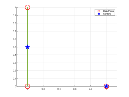
Figure 1: Visualization of the global solution to Example 5.1.

Example 5.2.

We consider a simple unconstrained example to verify Algorithm 4 using non-trivial Minkowski gauges and illustrate the differing global solutions they produce. We examine 4 data points in $\mathbb{R}^{2}$ on the unit square: $a^{1}=(0,0),\;a^{2}=(1,0)\;a^{3}=(0,1)\;a^{4}=(1,1)$, and seek two centers $x^{1}$ and $x^{2}$. The three gauges are considered: the usual $\rho_{F}(x)=\|x\|_{2}$, along with $\rho_{F}(x)=\|x\|_{1}$ and $\rho_{F}(x)=\|x\|_{\infty}$. A visualization of the computed global solutions using Algorithm 4 is shown in Figure 2. Figure 2(a) corresponds to an exact global solution where one center is the Fermat-Torricelli point of the triangle formed by $a^{1},a^{2},a^{4}$, with other center at $a^{3}$. Permutations of the centers yield alternative global solutions. For $\rho_{F}(x)=\|x\|_{1}$, many global solutions exist, including $x^{1}\in[a^{3},a^{4}]$ and $x^{2}\in[a^{1},a^{2}]$ or $x^{1}\in[a^{1},a^{4}]$ and $x^{2}\in[a^{2},a^{3}]$. Figure 2(b) demonstrates algorithm 4 converging to one of these exact global solutions. For $\rho_{F}(x)=\|x\|_{\infty}$, figure 2(c) shows the exact global solution of $x^{1}=(0.5,0.5)$ and $x^{2}=a^{1}$, with other global solutions $x^{2}=a^{i}$ for $i=2,3,4$. In this example, we use $\lambda_{\text{start}}=1$, $\delta=0.5$, and random initial values within the square. This example shows that Algorithm 4 converges correctly for complex Minkowski gauges and demonstrates how different gauges can yield distinct solutions and clustering outcomes, even in simple cases.

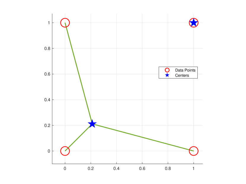
(a) $\rho_{F}(x)=\|x\|_{2}$

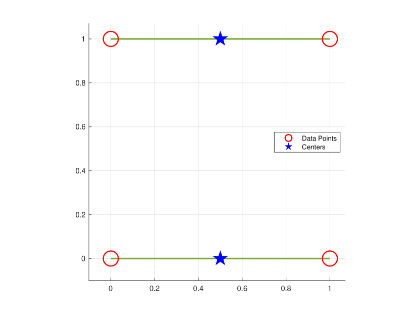
(b) $\rho_{F}(x)=\|x\|_{1}$

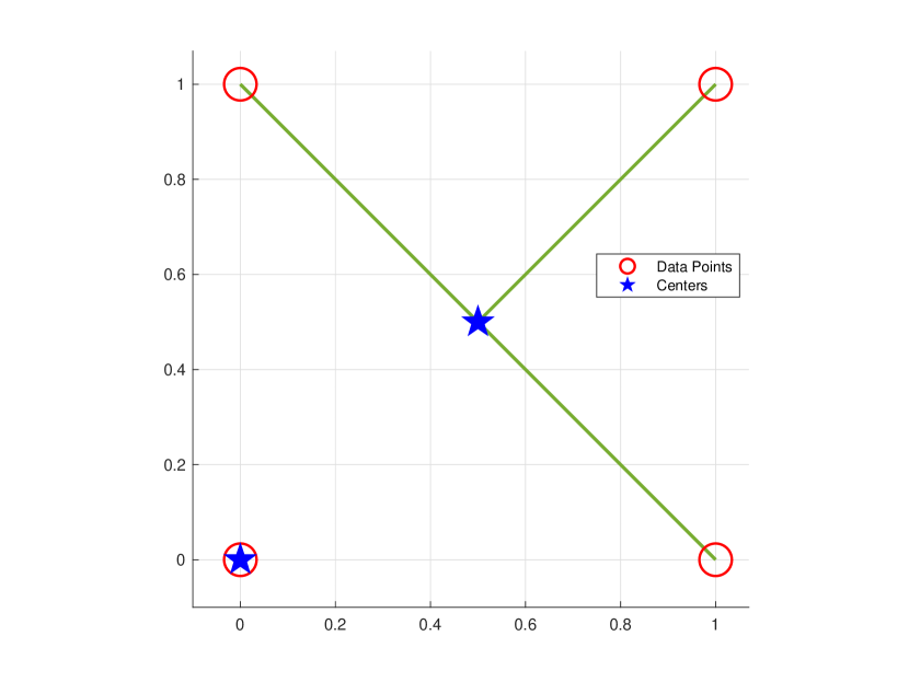
(c) $\rho_{F}(x)=\|x\|_{\infty}$

Figure 2: Visualization of the global solutions to Example 5.2.

Example 5.3.

We revisit Example 3 from [20], which tests 6 real data sets: WINE (178 instances in $\mathbb{R}^{13}$, 3 different cultivars), IRIS (150 observations in $\mathbb{R}^{4}$, 3 iris types), PIMA (768 observations in $\mathbb{R}^{8}$, predicting diabetes), IONOSPHERE (351 radar observations in $\mathbb{R}^{34}$), and the latitude/longitude of 1217 US cities with 3 centers. A visualization of the US cities global solution with $\rho_{F}(x)=\|x\|_{\infty}$ is shown in Figure 3. We compare Algorithm 5 from [20] with Algorithms 4 and 6, using the same $\mu$ values with suitable choices for $\lambda_{\text{skip}}$, $\lambda_{\text{start}}=1$ and $\delta=0.5$. Tables 2 and 1 present the average run-time and number of iterations over 100 runs, showing improvements across all norms. However, Table 1 shows that Algorithm 4 has slower run-time despite fewer iterations. When using Algorithm 6, see Table 2, we have both run-time and iteration improvement. Further discussion is provided in the next example.

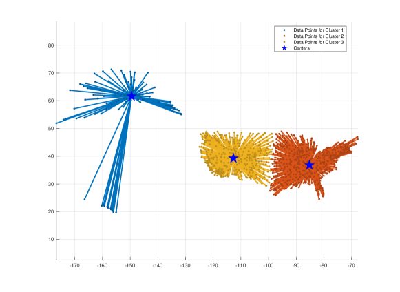
Figure 3: A visualization of the global solution to Example 5.3.

				$\rho_{F}(x)=\|x\|_{2}$		$\rho_{F}(x)=\|x\|_{1}$		$\rho_{F}(x)=\|x\|_{\infty}$
	m	n	k	Iteration
Ratio	Time
Ratio	Iteration
Ratio	Time
Ratio	Iteration
Ratio	Time
Ratio
Wine	178	13	3	1.31	0.65	1.54	0.73	1.41	0.58
Iris	150	4	3	1.69	0.79	1.61	0.61	1.23	0.56
PIMA	768	8	2	1.59	0.79	1.36	0.65	2.18	0.96
Ionosphere	351	34	2	1.42	0.82	1.05	0.46	1.40	0.65
USCity	1217	2	3	3.93	1.54	1.80	0.53	2.07	0.79

Table 1: DCA/aBDCA ratios for time and iterations in Example 5.3 using algorithm 4

				$\rho_{F}(x)=\|x\|_{2}$		$\rho_{F}(x)=\|x\|_{1}$		$\rho_{F}(x)=\|x\|_{\infty}$
	m	n	k	Iteration
Ratio	Time
Ratio	Iteration
Ratio	Time
Ratio	Iteration
Ratio	Time
Ratio
Wine	178	13	3	1.36	1.27	1.51	1.67	1.41	1.27
Iris	150	4	3	1.75	1.43	1.56	1.20	1.31	1.19
PIMA	768	8	2	2.02	1.41	1.35	1.13	2.09	1.67
Ionosphere	351	34	2	1.44	1.32	1.09	1.02	1.43	1.33
USCity	1217	2	3	4.13	3.71	1.77	1.65	2.06	1.91

Table 2: DCA/aBDCA ratios for time and iterations in Example 5.3 using algorithm 6

Example 5.4.

We consider an artificial example similar to Example 7.3 from [19], involving 1000 points within 4 circles, where 4 centers are found constrained to a single center circle (see in Figure 4). The parameters are $\sigma=10,\delta=0.25,\lambda_{\text{start}}=0.1$, $\lambda_{f}=10^{-3}$, $\lambda_{\text{skip}}=30$. Figures 6 and 6 compare adaptive BDCA and DCA using Algorithms 5 and 7 over 100 random initial values. The need for skipping becomes clear, as both show similar iteration improvements. However, performing algorithm 5 makes it 2/3 slower than DCA, while Algorithm 7 offers a run-time advantage. This can be explained by examining the line search step lengths in both BDCA versions.

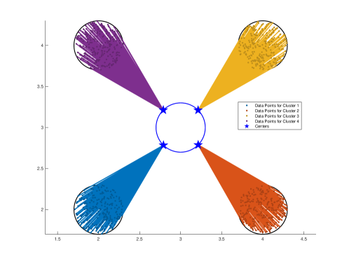
Figure 4: Visualization of the global solution to Example 5.4.

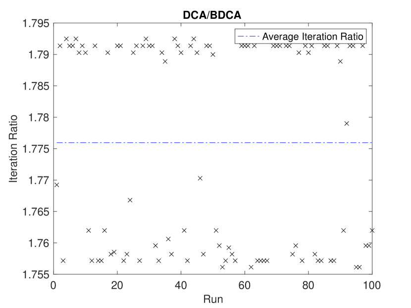
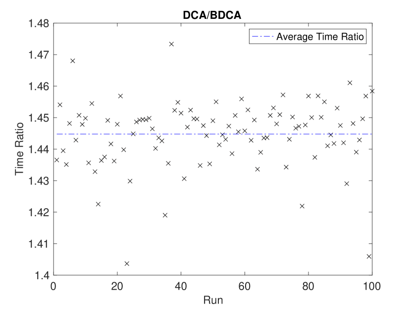
Figure 5: Iteration and time ratio comparison for Example 5.4 with algorithm 7.

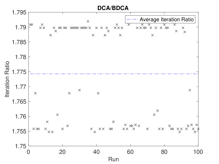
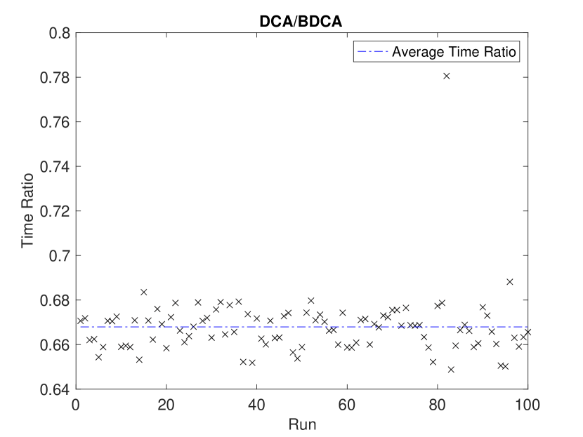
Figure 6: Iteration and time ratio comparison for Example 5.4 with algorithm 5

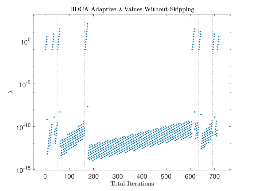
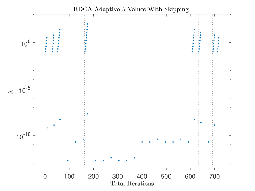
Figure 7: Line-search step lengths $\lambda$ for a single run of Example 5.4 using algorithm 5 (left), and algorithm 7 (right). Dashed vertical lines indicate outer loop iteration, adjusting $\tau$ and $\mu$.

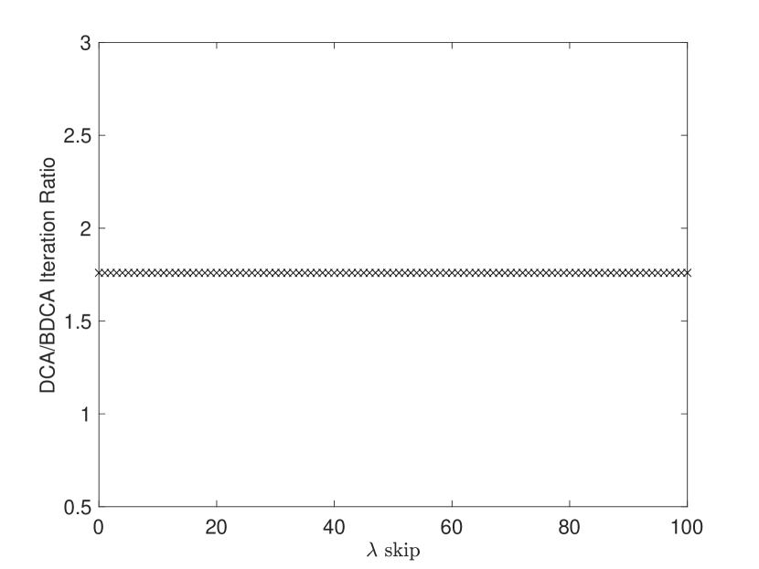
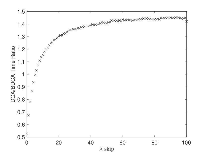
Figure 8: Average DCA/ aBDCA iteration and time ratio for varying values of $\lambda_{\text{skip}}$ in algorithm 7 for Example 5.4.

As shown in Figure 7, the step length $\lambda$ is only significant right after adjusting $\tau$ and $\mu$ and becomes negligible after a few iterations, making adaptive BDCA behave like basic DCA. By skipping the line search every 30 iterations when $\lambda$ falls below $10^{-3}$, we retain the benefits of line search without excessive cost. This pattern of narrow regions with non-trivial line search was consistent across all tested examples, proving the effectiveness of Algorithm 7 for MWP. However, such regions don’t always appear immediately after adjusting $\tau\text{ and }\mu$, as shown in Example 5.5 and Figure 11. This is why we need a skipping algorithm rather than switching to basic DCA when $\lambda$ falls below $\lambda_{f}$. Finally, Figure 8 shows that large values of $\lambda_{\text{skip}}$ in Algorithm 7 have no negative impact, and skipping leads to significant performance gains over DCA in this case.

Example 5.5.

We revisit Example 7.4 from [19], which uses real-world data consisting of the latitudes and longitudes of the 988 most-populated cities in the contiguous United States [26]. A visualization of the problem and its solution is provided in [19]. The parameters are $\sigma=100,\;\delta=0.25,\;\lambda_{\text{start}}=1,\;\lambda_{f}=10^{-3},\;\lambda_{\text{skip}}=100$. Figures 10 and 10 compare the performance of algorithms 5 and 7, using 100 random initial values. Skipping is again crucial: while both algorithms reduce the iteration count by approximately 1.7 times compared to DCA, algorithm 5 is 0.8 times slower due to the line search cost. With algorithm 7, however, we achieve a 1.6 run-time improvement over DCA. Figure 11 illustrates the line search step lengths for both versions. Again, distinct narrow regions emerge where line search improves adaptive BDCA, while for most iterations, adaptive BDCA behaves like DCA. Unlike previous examples, these regions occur throughout an inner loop with fixed $\tau$ and $\mu$ values. The skipping version effectively detects and activates the line search when necessary, maintaining similar iteration improvements to algorithm 5. Figure 12 shows the impact of varying $\lambda_{\text{skip}}$. The more complex nature of this problem is reflected in the noticeable sensitivity to $\lambda_{\text{skip}}$, but across a wide range of values, most yield a run-time improvement of around 1.6, as long as $\lambda_{\text{skip}}$ exceeds 20. This highlights the robustness of the algorithm to the choice of $\lambda_{\text{skip}}$.

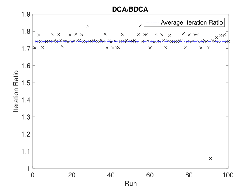
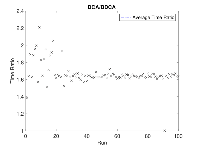
Figure 9: Iteration and time ratio comparison for Example 5.5 using algorithm 7.

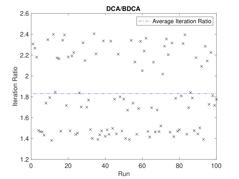
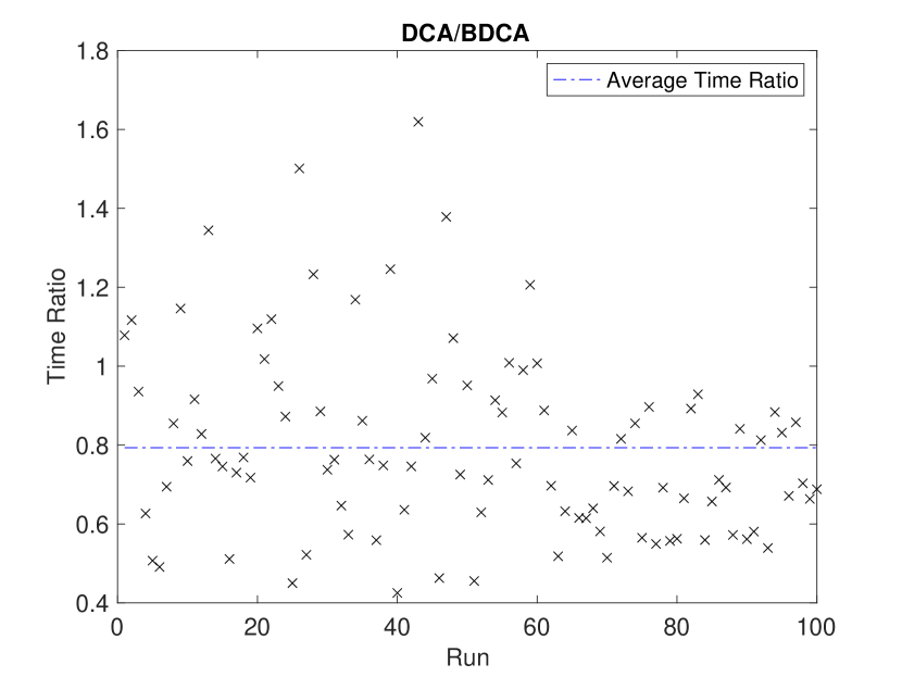
Figure 10: Iteration and time ratio comparison for Example 5.5 using algorithm 5.

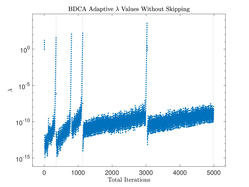
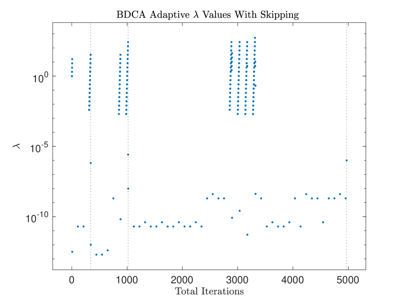
Figure 11: Line-search step lengths $\lambda$ for a single run of Example 5.5 using algorithm 5 (left) and algorithm 7 (right). Dashed vertical lines indicate outer loop iteration, adjusting $\tau$ and $\mu$.

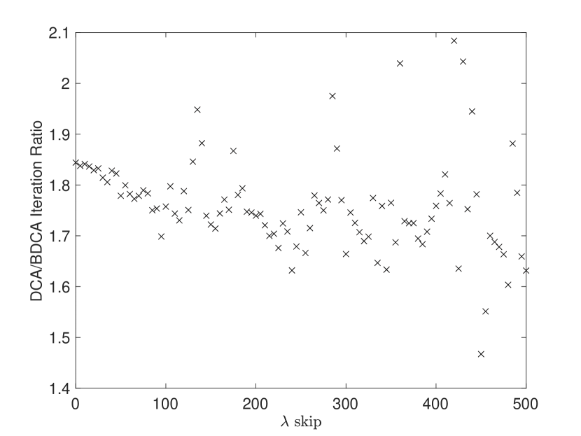
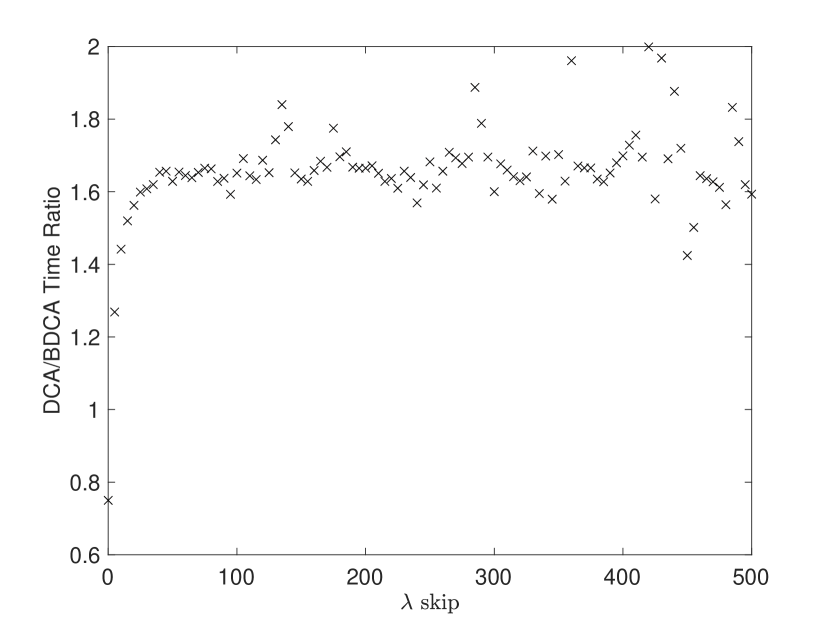
Figure 12: Average DCA/aBDCA iteration and time ratio for Example 5.5 for varying values of $\lambda_{\text{skip}}$ in algorithm 7.

Example 5.6.

We test our algorithm using the EIL76 dataset from the Traveling Salesman Problem Library [21], seeking 2 centers constrained to lie within:

1. Circles with radii 7 and 4.5, centered at $\left(30,40\right)\text{ and }\left(32,37\right)$, and the rectangle with vertices $\{\left(40,30\right),\left(40,40\right),\left(30,40\right),\left(30,30\right)\}$
   

2. Circles with radii 7,7, and 5, centered at $\left(35,20\right)$, $\left(45,20\right)$ and $\left(40,15\right)$.

A visualization of the problem and its solution is shown in Figure 13. The parameters are $\sigma=100,\;\delta=0.85,\;\lambda_{\text{start}}=1,\;\lambda_{f}=10^{-3},\;\lambda_{\text{skip}}=150$. Only the results using Algorithm 7 are presented, as Algorithm 5, similar to previous examples, fails to provide a run-time improvement. Figure 14 shows the relative performance of Algorithm 7 compared to DCA, with a moderate run-time improvement of about 1.34 times. In addition, Figure 15 shows that a wide range of $\lambda_{\text{skip}}$ values still result in a speed-up over DCA.

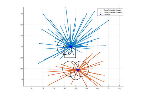
Figure 13: Visualization of the global solution to Example 5.6.

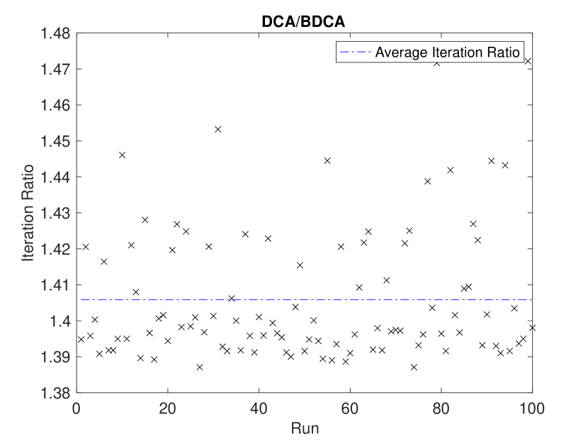
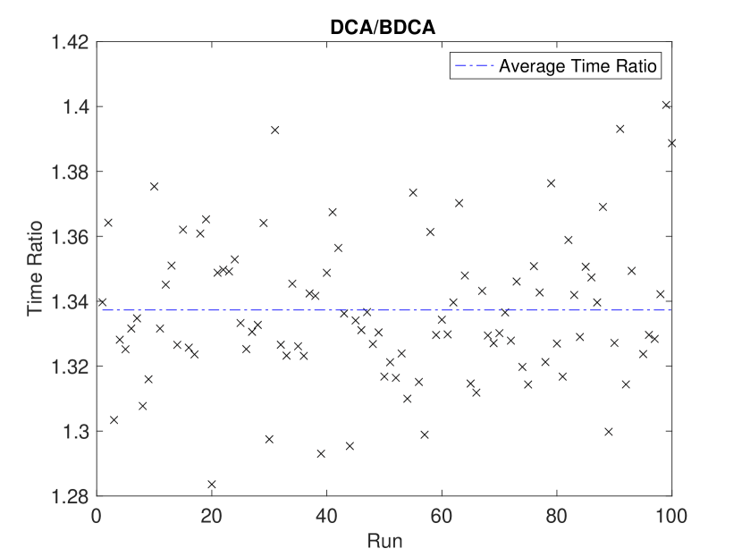
Figure 14: Iteration and time ratio comparison for Example 5.6 using algorithm 7.

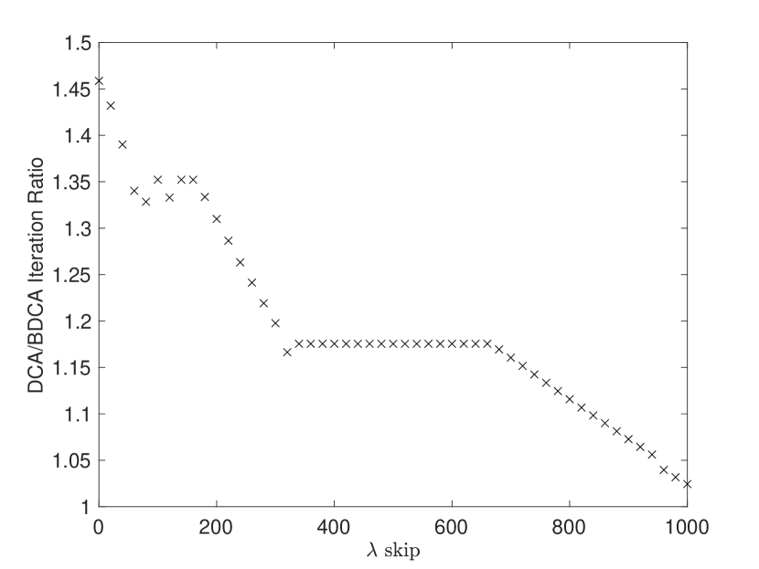
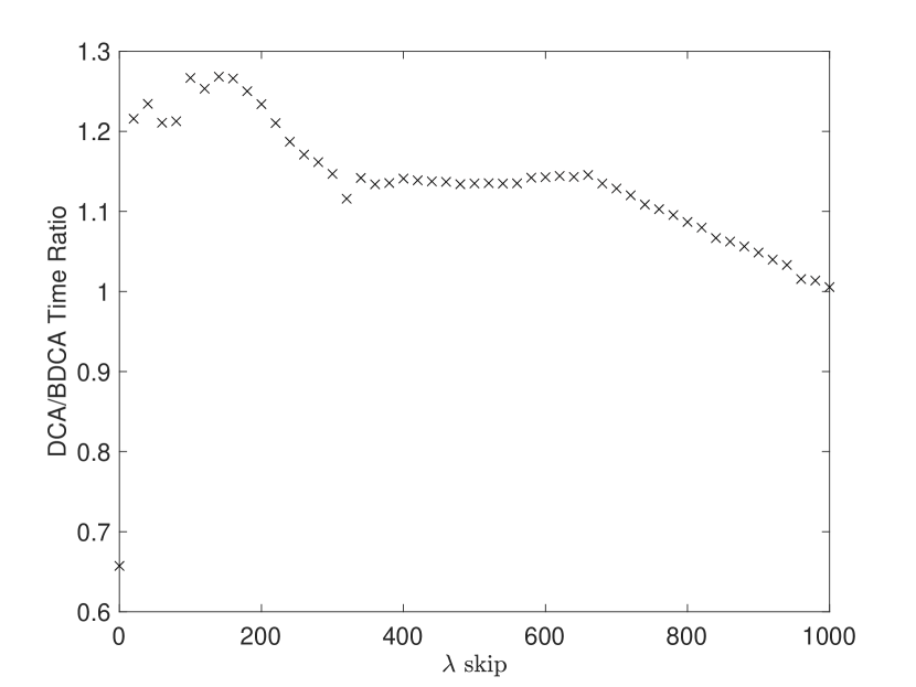
Figure 15: Average DCA/aBDCA iteration and time ratio for Example 5.6 using varying values of $\lambda_{\text{skip}}$ in algorithm 7.

6 Conclusion

In this paper, we provide details exploring the fundamental qualitative properties of the Generalized Multi-source Weber Problem using the Minkowski gauge function instead of the Euclidean norm. We show that the problem always admits a global solution and that the global solution set is compact. In addition, we introduce a concept of a local solution and provide necessary and sufficient conditions for its existence. From a numerical perspective, we propose an adaptive BDCA with skipping technique that improves both iteration counts and run-time. Unlike the results in [6], adaptive BDCA struggles with GMWP. While reducing iterations compared to DCA, it suffers from slower run times due to the line search cost. Our new algorithm incorporates a skipping mechanism to avoid unnecessary line searches, which improves both iteration counts and run-time. The skipping parameter is robust, with a wide range of effective values for each problem. Future work will focus on developing an advanced skipping method for more complex problems and testing the algorithm on large-scale, higher-dimensional problems.

References

- [1] L. T. H. An, M. T. Belghiti, and P. D. Tao, A new efficient algorithm based on DC programming and DCA for clustering. J. Global Optim. 37.4 (2007), pp. 593–608.
- [2] L. T. H. An and P. D. Tao, DC programming and DCA: thirty years of developments. Math. Program. 169.1 (2018), pp. 5–68.
- [3] L. T. H. An and P. D. Tao, The DC (difference of convex functions) programming and dca revisited with dc models of real world nonconvex optimization problems. Annal. Oper. Res. 133.1 (2005), pp. 23–46.
- [4] F. J. Aragón-Artacho, R. Campoy, and P. T. Vuong, The boosted DC algorithm for linearly constrained DC programming. Set-Valued and Var. Anal. 30.4 (2022), pp. 1265–1289.
- [5] F. J. Aragón-Artacho, R. M. T. Fleming, and P. T. Vuong, Accelerating the DC algorithm for smooth functions. Math. Program. 169.1 (2018), pp. 95–118.
- [6] F. J. Aragón-Artacho and P. T. Vuong, The boosted difference of convex functions algorithm for nonsmooth functions. SIAM J. Optim. 30.1 (2020), pp. 980–1006.
- [7] G. Colombo and P. R. Wolenski, The subgradient formula for the minimal time function in the case of constant dynamics in Hilbert space. J. Global Optim. 28 (2004), pp. 269–282.
- [8] T. H. Cuong, N. Thien, J.-C. Yao, and N. D. Yen, Global solutions of the multi-source Weber Problems. J. Nonlinear Convex Anal. 24.4 (2023), pp. 669–680.
- [9] T. H. Cuong, C.-F. Wen, J.-C. Yao, and N. D. Yen, Local solutions of the multi-source Weber problem. Optimization (2024), pp. 1–15.
- [10] T. H. Cuong, J.-C. Yao, and N. D. Yen, Qualitative properties of the minimum sum-of-squares clustering problem. Optimization 69.9 (2020), pp. 2131–2154.
- [11] N. T. V. Hang and N. D. Yen, On the problem of minimizing a difference of polyhedral convex functions under linear constraints. J. Optim. Theory Appl. 171 (2016), pp. 617–642.
- [12] J-B. Hiriart-Urruty and C. Lemaréchal, Fundamentals of convex analysis. Springer Berlin Heidelberg, 2001.
- [13] H. W. Kuhn, A note on Fermat’s problem. Math. Program. 4 (1973), pp. 98–107.
- [14] V. S. T. Long, A new notion of error bounds: necessary and sufficient conditions. Optim. Letters. 15.1 (2021), pp. 171–188.
- [15] V. S. T. Long, N. M. Nam, J. Sharkansky, and N. D. Yen, Qualitative properties of k-center problems. Submitted (2024).
- [16] H. Martini, K.J. Swanepoel, and G. Weiss, The Fermat–Torricelli prob- lem in normed planes and spaces. J. Optim. Theory Appl. 115.2 (2002), pp. 283–314.
- [17] B. S. Mordukhovich and N. M. Nam, An easy path to convex analysis and applications. Second edition, Cham: Springer International Publishing, 2023.
- [18] B. S. Mordukhovich and N. M. Nam, Applications of variational analysis to a generalized Fermat–Torricelli problem. J Optim. Theory Appl. 148.3 (2010), pp. 431–454.
- [19] N. M. Nam, N. T. An, S. Reynolds, and T. Tran, Clustering and multifacility location with constraints via distance function penalty methods and DC programming. Optimization 67.11 (2018), pp. 1869–1894.
- [20] N. M. Nam, R. B. Rector, and D. Giles, Minimizing differences of convex functions with applications to facility location and clustering. J. Optim. Theory Appl. 173.1 (2017), pp. 255–278.
- [21] Gerhard Reinelt, TSPLIB—A Traveling Salesman Problem Library. ORSA Journal on Computing 3.4 (1991), pp. 376–384.
- [22] R. T. Rockafellar, Convex analysis. Princeton University Press, 1997.
- [23] P. D. Tao and L. T. H. An, A DC optimization algorithm for solving the trust-region subproblem. SIAM J. Optim. 8.2 (1998), pp. 476–505.
- [24] P. D. Tao and L. T. H. An, Convex analysis approach to DC programming: theory, algorithm and applications. Acta Math. Vietnamica 22.1 (1997), pp. 289–355.
- [25] P. D. Tao and E.B. Souad, Algorithms for solving a class of nonconvex op- timization problems. Mathematics for Optimization 129.1 (1986), pp. 249– 271.
- [26] United States Cities Database. 2017.