Induced gravitational waves, metastable cosmic strings and primordial black holes in GUTs

Abstract

We explore the cosmological and astrophysical implications of a realistic hybrid inflation model based on flipped $SU(5)$. The model contains superheavy metastable cosmic strings arising from a waterfall field that encounters a limited number of $e$-foldings during the inflationary phase. In addition to the gravitational waves emitted by the metastable strings, there also appear scalar induced gravitational waves linked to the waterfall phase transition. These two independent sources of gravitational waves can yield a combined spectrum that is compatible with the recent PTA measurements, and with additional features that can be probed in future experiments. We also show the appearance of primordial black holes with mass on the order of $10^{26}$ g from the waterfall phase transition, and with an abundance that can be tested in the gravitational lensing experiments.

Dedicated to the memory of our dear friend and collaborator George Lazarides. George was a larger than life figure as well as an outstanding theoretical physicist, and he will be sorely missed.

1 Introduction

Grand unified theories (GUTs) predict proton decay [1, 2, 3], and superheavy magnetic monopoles [4, 5] that may survive inflation and occur at an observable level [6, 7]. Other topological defects such as domain walls, cosmic strings, intermediate mass monopoles and various composite structures [8, 9, 10, 11, 12, 13] can appear in GUTs, depending on the symmetry breaking patterns, with rank greater than four. Detecting such topological defects would be one of the most spectacular confirmation of the physics beyond the Standard Model (BSM). Topologically stable magnetic monopoles can be present at an observable level provided that their density is diluted during inflation by a suitable number of $e$-foldings in order to satisfy observational constraints from experiments such as MACRO [14], IceCube [15] and ANTARES [16]. For example, intermediate scale monopoles in GUTs such as $SO(10)$ should experience $N_{M}\gtrsim 13$ number of $e$-foldings during inflation [6, 7]. Superheavy metastable cosmic strings (MSS) [17, 18, 19, 20, 21, 22, 23, 24, 13] with a dimensionless string tension parameter $G\mu\sim 10^{-6}$ emit a gravitational wave (GW) spectrum that can explain the NANOGrav 15 year [25, 26, 27] and other pulsar timing array data [28, 29, 30, 31]. However, to evade the LIGO-VIRGO constraint on the GW spectrum at the decaHertz frequencies [32], the strings should be partially inflated by about 20-45 $e$-foldings [18] or experience an early matter dominated era [19]. Other hybrid topological structures, such as quasistable strings (QSS) and walls bounded by strings (WBS), can emit also gravitational waves compatible with the NANOGrav 15 year results provided that the superheavy strings and monopoles experience an appropriate amount of inflation [33, 34].

A recent hybrid inflation model based on flipped $SU(5)$ [18] provides a recipe to entirely inflate the $SU(5)$ superheavy monopoles, but the associated cosmic strings, produced during the waterfall phase, only experience a limited number of $e$-foldings. This kind of intermediate waterfall phase also may produce enhanced primordial curvature perturbations [35, 36, 37, 7], which can result in the generation of an additional source of GWs, commonly referred to as the scalar induced gravitational waves (SIGW). Finally, the enhanced scalar perturbations can give rise to primordial black holes (PBHs) which may be present at an observable level.

In this article, we investigate the possibility that the stochastic gravitational wave background accessible in the pulsar timing array experiments is a superposition of the emission from the two distinct sources above, namely the SIGW and the metastable cosmic string gravitational waves (MSSGW). We focus on the flipped $SU(5)$ hybrid inflation model [18], where the necessity that the cosmic strings are partially inflated during an intermediate waterfall phase, motivates us to look for another region of the parameter space that allows for the appearance of both SIGWs and MSSGW in explaining the PTA results. The $SU(5)$ symmetry breaking scale is $\approx 5\times 10^{16}$ GeV, and the corresponding proton lifetime is estimated to be of order $10^{37}$ yrs, which is beyond the reach of the Hyper-Kamiokande experiment [38]. We explore a scenario where the PBHs are produced with an abundance that makes them detectable in the gravitational lensing experiments. Although we focus here on a specific GUT gauge group, we should emphasize that our considerations based on hybrid inflation and waterfall phase transitions can be readily extended to other GUT models. The emission of gravitational waves from two distinct sources and the appearance of primordial black holes is a salient feature of our hybrid inflation model.

The paper is structured as follows. In section 2 we briefly review the flipped $SU(5)$ hybrid inflation model in Ref. [18] and the production of metastable strings during the waterfall transition. We study the inflationary dynamics and observables in section 3, and present representative benchmark points. In section 4, we discuss the scenario with two distinct sources of GWs and compatibility with the PTA data as well as the LIGO-VIRGO data. In section 5, we study the production of PBHs during the waterfall phase transition, and our conclusions are summarized in section 6.

2 Metastable cosmic strings from flipped $SU(5)$ model and hybrid inflation

The flipped $SU(5)$ ($SU(5)\times U(1)_{X}$) model in Ref. [18] is an interesting candidate for our study of multiple sources of stochastic gravitational waves background, with the following symmetry breaking chain:

$$SU(5)\times U(1)_{X} \xrightarrow[]{\left<\Phi\right>} SU(3)_{c}\times SU(2)_{L}\times U(1)_{Z}\times U(1)_{X}$$ (2.1)

$$\xrightarrow[]{\left<\Psi\right>} SU(3)_{c}\times SU(2)_{L}\times U(1)_{Y},$$

where $\Phi\equiv\mathbf{24}_{H}(0)$ and $\Psi\equiv\mathbf{10}_{H}(-1)$. The gauge invariant terms in the scalar potential, realizing the symmetry breaking chain (2.1) and relevant to inflation, are given as follows:

$$V \supset V_{0}-\mu_{\Phi}^{2}\,tr(\Phi^{2})-\dfrac{\mu_{1}}{3}\,tr(\Phi^{3})+\dfrac{\lambda_{1}}{4}\,tr(\Phi^{4})+\lambda_{2}\,[tr(\Phi^{2})]^{2}-\dfrac{\mu_{\Psi}^{2}}{2}\,tr(\Psi^{\dagger}\Psi)+\dfrac{\lambda_{3}}{4}\,[tr(\Psi^{\dagger}\Psi)]^{2}$$ (2.2)

$$+\dfrac{\lambda_{4}}{4}\,tr(\Psi^{\dagger}\Psi\Psi^{\dagger}\Psi)+\lambda_{5}\,tr(\Psi^{\dagger}\Phi^{2}\Psi)+\lambda_{6}\,tr(\Psi^{\dagger}\Psi)\,tr(\Phi^{2})+\mu_{2}\,tr(\Psi^{\dagger}\Phi\Psi)$$

$$+\dfrac{m^{2}}{2}S^{2}+\lambda_{7}S^{2}tr(\Psi^{\dagger}\Psi)-\lambda_{8}S^{2}tr(\Phi^{2})\,,$$

where the adjoint representation $\Phi^{\alpha}_{\,\,\beta}\equiv\phi_{a}(T^{a})^{\alpha}_{\,\beta}$, with $T^{a}$ being the $SU(5)$ generators, and the 10-plet $\Psi$ is a $5\times 5$ complex antisymmetric matrix $\Psi^{\alpha\beta}$. The sum over repeated indices is understood, with $a,b,c,\cdots=1,2,\cdots 24$, and $\alpha,\beta,\cdots=1,2,\cdots 5$. The real singlet scalar $S$ represents the inflaton, and we do not include linear, cubic and quartic terms in $S$ assuming that they are adequately small, and hence do not affect the inflation dynamics. The constant vacuum energy $V_{0}$ is added in order to guarantee a zero cosmological constant in the desired potential minimum.

With the symmetry breaking chain (2.1), $SU(5)$ is broken first via the 24-plet $\Phi$ yielding magnetic monopoles carrying $SU(3)_{c}$, $SU(2)_{L}$ and $U(1)_{Z}$ magnetic fluxes, which are entirely inflated away. The subsequent symmetry breaking $U(1)_{Z}\times U(1)_{X}\to U(1)_{Y}$ yields cosmic strings which can decay via the quantum-tunneling of monopole-antimonopole pairs [18]. The decay width per unit length of the string is expressed as [39]

$$\Gamma_{d}=\frac{\mu}{2\pi}\exp{\left(-\pi m_{M}^{2}/\mu\right)},$$ (2.3)

with $m_{M}$ being the monopole mass and $\mu$ the string tension. The superheavy metastable strings can produce gravitational waves compatible with the NANOGrav 15 year data and the constraint from LIGO-VIRGO third run results if: i) the dimensionless string tension parameter $G\mu$ is of order $10^{-6}$ with a metastability factor $\sqrt{\kappa}\equiv m_{M}/\sqrt{\mu}\sim 8$, and ii) the strings experience a limited number of $e$-foldings before the end of inflation [18].

As explained in Ref. [18], the scalar potential (2.2) provides a hybrid inflation model where the Higgs field $\Psi$ plays the role of the waterfall field that is frozen at the origin during inflation until $S$ reaches a critical value $S_{c}$, at which point the waterfall phase transition is triggered. The Higgs field $\Phi$ is shifted from the origin, following a field dependent minimum during inflation until the time at which $S=S_{c}$. The inflationary potential during this phase has the form

$$V_{\rm inf} = V_{0}-\dfrac{m_{\phi}^{2}}{2}\,\phi^{2}+\dfrac{\beta_{\phi}}{4}\,\phi^{4}-\dfrac{m_{\psi}^{2}}{2}\,\psi^{2}+\dfrac{\beta_{\psi}}{4}\,\psi^{4}+\frac{\beta_{\psi\phi}}{2}\,\psi^{2}\phi^{2}+\dfrac{m^{2}}{2}S^{2}+\frac{\beta_{S\psi}}{2}\,S^{2}\,\psi^{2}-\frac{\beta_{S\phi}}{2}\,S^{2}\,\phi^{2}\,,$$

where $\phi$ and $\psi$ represent the real canonically normalized components of the scalar fields $\Phi$ and $\Psi$ which acquire the VEVs. The superrenormalizable terms with coefficients $\mu_{1}$ and $\mu_{2}$ are suitably controlled such that their effects on the dynamics are negligible, and for simplicity we set $\mu_{1}=\mu_{2}=0$ in Eq. (2.2). Also, we assume that all of the remaining coefficients are real. The components of $\Phi$ and $\Psi$ are fixed at zero during and after inflation, and the parameters $m_{\phi},m_{\psi},\beta_{\phi},\beta_{\psi},\beta_{\psi\phi},\beta_{S\phi},\beta_{S\psi}$ can be expressed in terms of the original potential parameters in Eq. (2.2). The constant vacuum energy $V_{0}$ satisfies

$$V_{0}=\dfrac{1}{4}\left(m_{\psi}^{2}v_{\psi}^{2}+m^{2}_{\phi}v_{\phi}^{2}\right),$$ (2.5)

where $v_{\psi}$ and $v_{\phi}$ are the vacuum expectation values of $\psi$ and $\phi$ respectively. The inflation trajectory in the $(\psi,\phi)$ plane is given by [40, 18, 7]

$$(\psi,\phi)=\left(0\,,\,\sqrt{\frac{m_{\phi}^{2}+\beta_{S\phi}S^{2}}{\beta_{\phi}}}\right)\,.$$ (2.6)

Th standard hybrid inflation tree level potential [41] is then modified to a hill-top shaped one [40, 18, 7], with the tree level effective potential given by

$$V_{\text{inf}}(\widetilde{S})=\widetilde{V}_{0}\left(1+\widetilde{S}^{2}-\gamma\,\widetilde{S}^{4}\right),$$ (2.7)

where

$$\widetilde{V}_{0}\equiv V_{0}-\dfrac{m_{\phi}^{4}}{4\beta_{\phi}}\,,\hskip 14.22636pt\widetilde{S}\equiv\sqrt{\dfrac{\eta_{0}}{2}}\,S\,,\hskip 14.22636pt\eta_{0}\equiv\frac{m^{2}\beta_{\phi}-m_{\phi}^{2}\beta_{S\phi}}{\widetilde{V}_{0}\,\beta_{\phi}}\,,\hskip 14.22636pt\gamma\equiv\frac{\beta_{S\phi}^{2}}{\eta_{0}^{2}\widetilde{V}_{0}\,\beta_{\phi}}\,,$$ (2.8)

and the critical value of the inflaton field $S_{c}$, at which the waterfall is triggered is given by

$$S_{c}=\sqrt{\frac{\beta_{\phi}m_{\psi}^{2}-\beta_{\psi\phi}m_{\phi}^{2}}{\beta_{\psi\phi}\beta_{{S\phi}}+\beta_{\phi}\beta_{{S\psi}}}}\,.$$ (2.9)

The 1-loop Coleman-Weinberg (CW) correction to the tree level inflation potential (2.7) may yield a significant change to the inflation observables, since the waterfall fields have inflaton dependent masses during inflation. However, it was shown in Ref.[18] that the CW radiative correction is under control and yields a tiny contribution to the total potential if we introduce an extra pair of fermionic $10_{F_{1}}$, $\overline{10}_{F_{2}}$, with $X=4,-4$ respectively. In our numerical calculations we choose values of the Yukawa couplings $Y_{S}\,S\,10_{F_{1}}\overline{10}_{F_{2}}$ and $Y_{\Phi}\,\Phi\,10_{F_{1}}\overline{10}_{F_{2}}$, such that the CW correction is very small compared to the tree level inflation potential (2.7).

After reaching the global minimum of the scalar potential (2), the inflaton field $S$ and the waterfall fields $\phi$ and $\psi$ start to oscillate around their respective minima and decay, such that the reheating phase starts. The inflaton field $S$ and the adjoint scalar field $\phi$ decay to the SM Higgs doublets $\cal H$ via the couplings $\delta_{1}\,S\,{\cal H}^{\dagger}{\cal H}$ and $\delta_{2}\,\phi\,{\cal H}^{\dagger}{\cal H}$. On the other hand, the scalar field $\psi$ decay produces right handed neutrinos via the non-renormalizable coupling $\frac{f}{M_{\rm Pl}}10_{F}10_{F}10_{H}^{\dagger}\,10_{H}^{\dagger}$. The reheating temperature $T_{r}$ consistent with the observables is less than or of order $10^{12}$ GeV [18].

Our aim is to shed light on representative points in an interesting region of the parameter space with intermediate waterfall phase [42, 43, 36, 18, 7] that continues for $\sim 20-40$ $e$-foldings, with a significant enhancement of the curvature power spectrum from the waterfall phase transition. In this case, SIGWs are generated by second order effects in perturbation theory. Moreover, primordial black holes may be produced with a significant abundance. Moreover, the metastable cosmic strings produced during the waterfall phase are partially inflated, and they constitute another source of gravitational waves (MSSGW) in addition to the SIGWs. We explore the interplay between the two sources of gravitational waves and the potential production of PBHs in the next sections.

3 Inflationary dynamics and observables

We define the Hubble slow-roll parameters as follows

$$\epsilon_{H} \equiv \dfrac{1}{2H^{2}}\sum_{n=1}^{3}{\dot{\varphi}_{n}}^{2}=\dfrac{1}{2}\sum_{n=1}^{3}{\varphi_{n}^{\prime}}^{2}\,,\,\,\,\,\,\eta_{H}\equiv\dfrac{\epsilon_{H}^{\prime}}{\epsilon_{H}}\,,$$ (3.1)

with the Hubble parameter $H$ given by

$$H^{2}=\left(\frac{\dot{a}}{a}\right)^{2}=\dfrac{1}{3M^{2}_{\rm Pl}}\left[\dfrac{1}{2}\sum_{n=1}^{3}\dot{\varphi}_{n}^{2}+V(\varphi_{n})\right],$$ (3.2)

where $a$ is the scale factor. Here, a dot denotes the derivative with respect to the cosmic time $t$, and a prime denotes the derivative with respect to the number of $e$-foldings variable $N$. The classical field dynamics is governed by the Klein-Gordon equations which can be recast in the form

$$\varphi_{n}^{\prime\prime}+\left(3-\epsilon_{H}\right)\varphi_{n}^{\prime}+\left(3-\epsilon_{H}\right)\dfrac{V_{n}}{V}=0\,,$$ (3.3)

where $n$ stands for $S,\psi,\phi$, and $V_{n}$ is the derivative of the potential with respect to $\varphi_{n}$. Denoting the Bardeen potentials by $\Phi_{\text{B}}$ and $\Psi_{\text{B}}$, the perturbed metric takes the form

$$ds^{2}=a(\tau)^{2}\left[-(1+2\Phi_{\text{B}})d\tau^{2}+\left(1-2\Psi_{\text{B}}\right)\delta_{ij}\,dx^{i}dx^{j}\right],$$ (3.4)

where $\tau$ is the conformal time defined by $dt\equiv ad\tau$. The evolution of the scalar field perturbations $\delta\varphi_{n}$ and $\Phi_{\text{B}}$ is described by the following equations [44, 45, 7]

$$\delta\varphi_{n}^{{}^{\prime\prime}}+(3-\epsilon_{H})\delta\varphi_{n}^{{}^{\prime}}+\dfrac{1}{H^{2}}\sum_{m=1}^{3}V_{nm}\delta\varphi_{m}+\dfrac{k^{2}}{a^{2}H^{2}}\delta\varphi_{n} = 4\Phi_{\text{B}}^{{}^{\prime}}\,\varphi^{\prime}_{n}-\dfrac{2\,\Phi_{\text{B}}}{H^{2}}V_{n},$$ (3.5)

$$\Phi^{{}^{\prime\prime}}_{\text{B}}+(7-\epsilon_{H})\,\Phi^{{}^{\prime}}_{\text{B}}+\left(2\dfrac{V}{H^{2}}+\dfrac{k^{2}}{a^{2}H^{2}}\right)\Phi_{\text{B}} = -\dfrac{1}{H^{2}}\sum_{m=1}^{3}V_{m}\,\delta\varphi_{m},$$ (3.6)

where $k$ is the co-moving wave vector, and the initial conditions at $N=N_{\rm ic}$ are given by [44, 45, 7]:

$$\delta\varphi_{n}(k,N_{\rm ic}) = \dfrac{1}{a\,\sqrt{2k}},$$ (3.7)

$$\delta\varphi_{n}^{{}^{\prime}}(k,N_{\rm ic}) = -\dfrac{1}{a\,\sqrt{2k}}\left(1+i\dfrac{k}{a\,H}\right),$$ (3.8)

$$\Phi_{\text{B}}(k,N_{\rm ic}) = \dfrac{1}{2\left(\epsilon_{H}-\dfrac{k^{2}}{a^{2}\,H^{2}}\right)}{{\sum}}_{m=1}^{3}\left(\varphi_{m}^{{}^{\prime}}\delta\varphi_{m}^{{}^{\prime}}+3\varphi_{m}^{{}^{\prime}}\delta\varphi_{m}+\dfrac{1}{H^{2}}V_{m}\,\delta\varphi_{m}\right),$$ (3.9)

$$\Phi_{\text{B}}^{{}^{\prime}}(k,N_{\rm ic}) = {{\sum}}_{m=1}^{3}\dfrac{1}{2}\varphi_{m}^{{}^{\prime}}\delta\varphi_{m}-\Phi_{\text{B}}\,.$$ (3.10)

The scalar power spectrum $P_{\zeta}(k)$ is then given by [44, 45, 7]

$$P_{\zeta}(k)=\dfrac{k^{3}}{2\pi^{2}}\left|\Phi_{\rm B}+\dfrac{\sum\limits_{m=1}^{3}\varphi^{\prime}_{m}\delta\varphi_{m}}{\sum\limits_{m=1}^{3}\varphi^{{}^{\prime}2}_{m}}\right|^{2}.$$ (3.11)

	$\widetilde{V}_{0}[M_{\rm Pl}^{4}]$	$\eta_{0}[M_{\rm Pl}^{-2}]$	$\gamma$
BP1	$1.982\times 10^{-11}$	$0.013$	$1.2$
BP2	$1.96\times 10^{-11}$	$0.013$	$0.9$

Table 1: Values of the parameters in the inflation potential (2.7).

	$m$	$m_{\psi}$	$m_{\phi}$	$\beta_{\psi}$	$\beta_{\phi}$	$\beta_{\psi\phi}$	$\beta_{S\psi}$	$\beta_{S\phi}$
BP1	$1.30\times 10^{12}$	$1.7\times 10^{15}$	$9.64\times 10^{14}$	1.52	0.095	$-0.379$	$9.97\times 10^{-8}$	$1.96\times 10^{-8}$
BP2	$1.27\times 10^{12}$	$8.308\times 10^{14}$	$6.025\times 10^{14}$	$0.15$	$0.02215$	$-0.058$	$2.5\times 10^{-8}$	$8.13\times 10^{-9}$

Table 2: Values of the parameters of the potential in Eq. (2), with dimensionful parameters given in GeV.

In our numerical simulations, integrating the perturbation equations and calculation of the primordial power spectrum, we use the method described in [44, 45, 36, 7]. In addition, we assume an initial displacement $\psi_{0}\sim H/(2\pi)$ at the time when $S=S_{c}$ [43, 36, 7]. The power spectrum is normalized at the pivot scale $k_{*}=0.05\,{\rm Mpc}^{-1}$ to satisfy the Planck constraints $P_{\zeta}(k_{*})=(2.099\pm 0.101)\times 10^{-9}$ [46, 47]. The total number of $e$-foldings during inflation is calculated, taking into account the thermal history of the universe, from the relation [48, 49, 50]:

$$\Delta N_{*}\simeq 61.5+\frac{1}{2}\mathrm{ln}\frac{\rho_{*}}{M_{\rm Pl}^{4}}-\frac{1}{3(1+\omega_{r})}\mathrm{ln}\frac{\rho_{e}}{M_{\rm Pl}^{4}}+\left(\frac{1}{3(1+\omega_{r})}-\frac{1}{4}\right)\mathrm{ln}\frac{\rho_{r}}{M_{\rm Pl}^{4}}\ ,$$ (3.12)

where $M_{\rm Pl}\approx 2.44\times 10^{18}$ GeV is the reduced Planck mass, $\rho_{*}=V(\widetilde{S}_{*})$ stands for the energy density of the universe when the pivot scale exits the horizon, $\rho_{e}=V(\widetilde{S}_{e})$ denotes the energy density at the end of inflation. The energy density at the reheating time is given by $\rho_{r}=(\pi^{2}/30)g_{*}T_{r}^{4}$, with $g_{*}=106.75$ being the effective number of massless degrees of freedom, corresponding to the SM spectrum. The quantity $w_{r}$ denotes the effective equation-of-state parameter from the end of inflation until reheating and we set it equal to $1/3$ [51]. The time at reheating $t_{r}$ is computed from the relation [52, 53]

$$T_{r}^{2}\approx\sqrt{\dfrac{45}{2\pi^{2}\,g_{*}}}\,\dfrac{M_{\rm Pl}}{t_{r}}.$$ (3.13)

	$v_{\phi}$	$v_{\psi}$	$M_{\psi^{\prime}}$	$M_{\phi^{\prime}}$	$M_{S}$
Obs(BP1)	$4\times 10^{16}$	$2\times 10^{16}$	$1.62\times 10^{15}$	$3.90\times 10^{16}$	$3.20\times 10^{12}$
Obs(BP2)	$6.48\times 10^{16}$	$4\times 10^{16}$	$9.5\times 10^{14}$	$2.6\times 10^{16}$	$2.83\times 10^{12}$

Table 3: Values of vevs and physical masses of the inflaton and waterfall fields in GeV. $M_{\phi^{\prime}}$ and $M_{\psi^{\prime}}$ are the eigenvalues of the mass matrix.

	$A_{s}$	$n_{s}$	$r$	$\Delta N_{*}$	$\Delta N_{c}$	$S_{*}[M_{\rm Pl}]$
Obs(BP1)	$2.04\times 10^{-9}$	$0.963$	$7.3\times 10^{-4}$	$56.07$	$32$	7.595
Obs(BP2)	$2.08\times 10^{-9}$	$0.966$	$1.3\times 10^{-3}$	$56.25$	$40$	8.660

Table 4: Predictions of CMB observables, and the total number of $e$-foldings during inflation $\Delta N_{*}$, and during waterfall $\Delta N_{c}$.

	$t_{c}$	$t_{e}$	$t_{r}$	$\omega_{r}$
Ob( BP1)	$1.8\times 10^{-35}$	$2.49\times 10^{-35}$	$4.45\times 10^{-28}$	1/3
Ob( BP2)	$1.54\times 10^{-36}$	$6.14\times 10^{-36}$	$9.42\times 10^{-33}$	1/3

Table 5: Time scales (in seconds) at different phases, and value of the equation of state parameter $w_{r}$. $t_{c}$, $t_{e}$, $t_{r}$ denote the cosmic times when $S=S_{c}$, at the end of inflation, and at reheating, respectively.

The benchmark points BP1 and BP2 correspond to metastable cosmic strings with dimensionless string tension $G\mu=8.44\times 10^{-6}$ and $G\mu=1.44\times 10^{-5}$ respectively. The Hubble parameter during the waterfall is $H\approx 2.\times 10^{-6}\,M_{\rm Pl}$. The curvature power spectrum is enhanced significantly at small scales due to the waterfall phase transition. The potential parameter values accounting for both SIGW and MSSGW are given in Tables (1) and (2), and the scalar fields vevs, physical masses and inflation observables are listed in Tables 3 and 4. The time scales at different phases are given in Table 5.

4 Gravitational waves from strings and scalar perturbations

As advocated above, the waterfall phase transition plays a dual role in our scenario. First, it is important to partially dilute the cosmic strings density such that the GW spectrum emitted from the sting network is compatible with the LVK bound. Secondly, as stated earlier, it enhances the curvature perturbations at small scales, and hence sources second order tensor perturbations, leading to the scalar induced gravitational waves. Assuming that the scalar induced GWs are produced during the radiation-dominated epoch, the spectrum is calculated from the formula [54, 55, 56, 57, 58]

$$\Omega_{\rm GW}^{\rm SI}h^{2}\approx 4.6\times 10^{-4}\left(\frac{g_{*,s}^{4}g_{*}^{-3}}{100}\right)^{\!-\frac{1}{3}}\!\int_{-1}^{1}{\rm d}x\int_{1}^{\infty}{\rm d}y\,\mathcal{P}_{\zeta}\left(\frac{y-x}{2}k\right)\mathcal{P}_{\zeta}\left(\frac{x+y}{2}k\right)F(x,y)\bigg{|}_{k=2\pi f}\,,$$ (4.1)

with $g_{*,s}\approx g_{*}$, and the function $F$ is defined as

$$F(x,y) = \frac{(x^{2}\!+\!y^{2}\!-\!6)^{2}(x^{2}-1)^{2}(y^{2}-1)^{2}}{(x-y)^{8}(x+y)^{8}}\times$$ (4.2)

$$\!\left\{\left[x^{2}-y^{2}+\frac{x^{2}\!+\!y^{2}\!-\!6}{2}\ln\left|\frac{y^{2}-3}{x^{2}-3}\right|\right]^{\!2}\!+\!\frac{\pi^{2}(x^{2}\!+\!y^{2}\!-\!6)^{2}}{4}\theta(y-\sqrt{3})\right\}.$$

The gravitational waves from the string network have been extensively studied in the literature [59, 60, 61, 62, 63, 64, 65, 66, 67, 68, 69, 70, 71, 72, 73, 74]. The metastable cosmic string network produces string loops with the number distribution given by [72]

$$n(l,t)=\frac{0.18}{t^{3/2}(l+\Gamma G\mu t)^{5/2}}\begin{cases}\Theta(0.18t-l)&\mathrm{for}\ \ t<t_{s}\\ e^{-\Gamma_{d}\left[l(t-t_{s})+\frac{1}{2}\Gamma G\mu(t-t_{s})^{2}\right]}\Theta(0.18t_{s}-\bar{l})&\mathrm{for}\ \ t>t_{s}\,\,\,,\end{cases}$$ (4.3)

where $\bar{l}=l+\Gamma G\mu(t-t_{s})$, $\Gamma\simeq 50$ is a numerical factor, and $t_{s}=1/\sqrt{\Gamma_{d}}$.

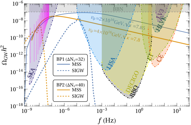
Figure 1: Gravitational waves from the metastable cosmic strings and the associated scalar induced gravitational waves. The gray region depicts the Big Bang Nucleosynthesis (BBN) bound [75] on the gravitational wave background for the BP1. The power-law integrated sensitivity curves [76, 77] for the ongoing and several proposed experiments, namely, HLVK [78], CE [79], ET [80], DECIGO [81], BBO [82, 83], LISA [84, 85] and SKA [86, 87] are shown.

The loops oscillate and radiate gravitational waves. The gravitational wave burst rate per unit spacetime is given by

$$\frac{d^{2}R}{dz\,dl}=N_{B}H_{0}^{-3}\phi_{V}(z)\frac{2n(l,t)}{l(1+z)}\Delta_{B}(f,l,z),$$ (4.4)

where $N_{B}$ is the average number of burst events per oscillation, $H_{0}$ denotes the Hubble parameter today, $\Delta_{B}(f,l,z)$ is the observable fraction of the bursts [62, 66, 67], and

$$\phi_{V}(z)=\frac{4\pi H_{0}^{3}r^{2}}{(1+z)^{3}{H}(z)},$$ (4.5)

with $r$ denoting the proper distance at redshift $z$. We assume that the cusp events provide the dominant contribution to the gravitational wave background. The wave form of the bursts from a cusp is expressed as [62],

$$h_{c}(f,l,z)=g_{c}\frac{G\mu l^{2/3}}{(1+z)^{1/3}r(z)}f^{-4/3},$$ (4.6)

where $g_{c}\simeq 0.85$ [32]. The gravitational wave background can be expressed as [66, 67]

$$\Omega_{\rm GW}^{\rm MSS}(f)=\frac{4\pi^{2}}{3H_{0}^{2}}f^{3}\int_{z_{*}}^{z_{F}}dz\int_{0}^{d_{H}}dl\,h^{2}_{c}(f,l,z)\frac{d^{2}R}{dz\,dl}\ ,$$ (4.7)

where $z_{F}$ and $z_{*}$ denote the redshifts at the time of string network formation and disappearance, and we have taken the particle horizon $d_{H}$ at redshift $z$ as the upper limit of integration on $l$.

Fig. 1 depicts the stochastic gravitational wave backgrounds sourced by the scalar perturbations and metastable strings. In the case of BP1, the metastable strings provide the dominant contribution to the gravitational wave background and can explain the NANOGrav 15 year data. Moreover, there will be a significant PBH dark matter abundance which can be observed in future lensing data (see Fig. 2). On the other hand, if the strings experience about 40 $e$-foldings of inflation and the PTA data can be explained around the nHz frequencies from a combination of the two sources. Moreover, the gravitational wave background displays a UV tail varying as $\Omega_{\rm GW}\propto f^{-1/3}$ starting from the $\mu$Hz frequencies which can be probed in several planned experiments such as $\mu$Ares [88], LISA [84, 85], DECIGO [81], BBO [82, 83], CE [79], and ET [80]. The $f^{-1/3}$ UV tail starts around the mHz frequency in the former case, and the background can be detected in the proposed and ongoing experiments including HLVK [78].

5 Primordial black holes

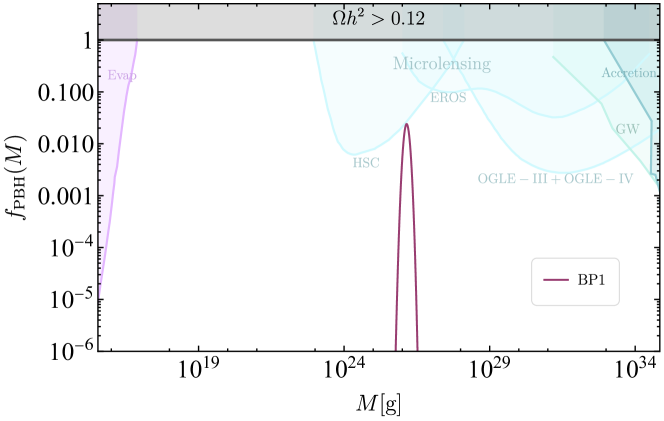
Figure 2: Primordial black holes fractional abundance for BP1. PBHs generated from BP2 have negligibly small abundance.

The enhancement in the power spectrum may result in the formation of PBHs if the density contrast $\delta\equiv\delta\rho/\rho$ exceeds a critical value $\delta_{c}(k)$ [89]. In this case, the PBHs mass fraction $\beta$ compared to the total mass of the universe can be evaluated using the Press-Schechter formalism, namely,

$$\beta(k)=\frac{1}{\sqrt{2\pi\sigma^{2}(k)}}\int^{\infty}_{\delta_{c}(k)}d\delta\,\exp\left(-\frac{\delta^{2}}{2\sigma^{2}(k)}\right)\,,$$ (5.1)

where $\sigma$ is the variance of the curvature perturbations which can be computed using the power spectrum and a window function with Gaussian distribution function $\widetilde{W}(x)=e^{-x^{2}/2}$ [90, 91],

$$\sigma^{2}\left(k\right)=\frac{16}{81}\int\frac{dk^{\prime}}{k^{\prime}}\left(\frac{k^{\prime}}{k}\right)^{4}P_{\zeta}(k^{\prime})\widetilde{W}\left(\frac{k^{\prime}}{k}\right),$$ (5.2)

with $0.4\lesssim\delta_{c}\lesssim 0.6$ [90, 92, 93, 94, 95, 96, 97, 98, 99, 100]. In terms of the co-moving wave number $k$, the PBH mass (in grams) is given by [101]

$$M_{\mathrm{PBH}}(k)=10^{18}\left(\frac{\gamma}{0.2}\right)\left(\frac{g_{*}(T_{f})}{106.75}\right)^{-1/6}\left(\frac{k}{7\times 10^{13}\,\mathrm{Mpc}^{-1}}\right)^{-2},$$ (5.3)

where we assume that PBHs are created during the radiation epoch, and $T_{f}$ represents the temperature at the time of their formation. The fractional abundance of PBHs, $f_{\rm PBH}\equiv\Omega_{\rm PBH}/\Omega_{\rm DM}$ has the form

$$f_{\rm PBH}(M_{\mathrm{PBH}})=\frac{\beta(M_{\mathrm{PBH}})}{8\times 10^{-16}}\left(\frac{\gamma}{0.2}\right)^{3/2}\left(\frac{g_{*}(T_{f})}{106.75}\right)^{-1/4}\left(\frac{M_{\mathrm{PBH}}\,}{10^{-18}\;\mathrm{grams}}\right)^{-1/2}\,,$$ (5.4)

where the factor $\gamma\sim 0.2$ represents the dependence on the gravitational collapse [102].

Figure 2 shows the predicted dark matter abundance of PBH with masses $M=2.3\times 10^{26}$ g ($1.15\times 10^{-7}\,M_{\odot}$) for BP1, that constitutes about 2% of the observed dark matter density which can be detected in the next generation of lensing experiments. For BP2, where the PTA results are explained in terms of SIGW and MSSGW, the corresponding PBH fractional abundance is extremely small. The shaded regions represent the various observational constraints on PBHs from black hole evaporation, accretion and GWs [103, 104, 105, 106, 107, 108, 109], and microlensing, including HSC, EROS and OGLE experiments [110].

6 Conclusions

We have explored the cosmological implications of a realistic flipped SU(5) model of hybrid inflation that yields superheavy metastable cosmic strings during the waterfall phase transition. We show how two sources of gravitational waves (GWs) appear, namely from the metastable cosmic strings (MSSGW), as well as from scalar perturbations associated with the waterfall field, often referred to as scalar induced gravitational waves (SIGW). We display representative benchmark points that allow for both types of GWs compatible with the recent PTA/NANOGrav results, and also with the LIGO-VIRGO third run. The spectrum features a $f^{-1/3}$ UV tail that can be detected in the proposed and ongoing experiments including HLVK. We also show that PBHs can be produced with mass of around $10^{26}$ g for the case where the MSSGW spectrum is the dominant one. Despite the relatively small dark matter fractional abundance of PBHs, their presence can be tested in the future lensing experiments.

References

- [1] H. Georgi and S.L. Glashow, Unity of All Elementary Particle Forces, Phys. Rev. Lett. 32 (1974) 438.
- [2] H. Fritzsch and P. Minkowski, Unified Interactions of Leptons and Hadrons, Annals Phys. 93 (1975) 193.
- [3] Q. Shafi, E(6) as a Unifying Gauge Symmetry, Phys. Lett. B 79 (1978) 301.
- [4] G. ’t Hooft, Magnetic Monopoles in Unified Gauge Theories, Nucl. Phys. B 79 (1974) 276.
- [5] G. Lazarides, M. Magg and Q. Shafi, Phase Transitions and Magnetic Monopoles in SO(10), Phys. Lett. B 97 (1980) 87.
- [6] R. Maji and Q. Shafi, Monopoles, strings and gravitational waves in non-minimal inflation, JCAP 03 (2023) 007 [2208.08137].
- [7] A. Moursy and Q. Shafi, Primordial monopoles, black holes and gravitational waves, JCAP 08 (2024) 064 [2405.04397].
- [8] T.W.B. Kibble, G. Lazarides and Q. Shafi, Walls Bounded by Strings, Phys. Rev. D 26 (1982) 435.
- [9] T.W.B. Kibble, G. Lazarides and Q. Shafi, Strings in SO(10), Phys. Lett. B 113 (1982) 237.
- [10] A. Vilenkin and A.E. Everett, Cosmic Strings and Domain Walls in Models with Goldstone and PseudoGoldstone Bosons, Phys. Rev. Lett. 48 (1982) 1867.
- [11] G. Lazarides and Q. Shafi, Monopoles, Strings, and Necklaces in and , JHEP 10 (2019) 193 [1904.06880].
- [12] G. Lazarides, Q. Shafi and A. Tiwari, Composite topological structures in SO(10), JHEP 05 (2023) 119 [2303.15159].
- [13] R. Maji, Q. Shafi and A. Tiwari, Topological structures, dark matter and gravitational waves in E6, JHEP 08 (2024) 060 [2406.06308].
- [14] MACRO collaboration, Final results of magnetic monopole searches with the MACRO experiment, Eur. Phys. J. C 25 (2002) 511 [hep-ex/0207020].
- [15] IceCube collaboration, Search for Relativistic Magnetic Monopoles with Eight Years of IceCube Data, Phys. Rev. Lett. 128 (2022) 051101 [2109.13719].
- [16] ANTARES collaboration, Search for magnetic monopoles with ten years of the ANTARES neutrino telescope, JHEAp 34 (2022) 1 [2202.13786].
- [17] S. Antusch, K. Hinze, S. Saad and J. Steiner, Singling out SO(10) GUT models using recent PTA results, Phys. Rev. D 108 (2023) 095053 [2307.04595].
- [18] G. Lazarides, R. Maji, A. Moursy and Q. Shafi, Inflation, superheavy metastable strings and gravitational waves in non-supersymmetric flipped SU(5), JCAP 03 (2024) 006 [2308.07094].
- [19] R. Maji and W.-I. Park, Supersymmetric U(1)B-L flat direction and NANOGrav 15 year data, JCAP 01 (2024) 015 [2308.11439].
- [20] W. Ahmed, M.U. Rehman and U. Zubair, Probing stochastic gravitational wave background from strings in light of NANOGrav 15-year data, JCAP 01 (2024) 049 [2308.09125].
- [21] A. Afzal, Q. Shafi and A. Tiwari, Gravitational wave emission from metastable current-carrying strings in E6, Phys. Lett. B 850 (2024) 138516 [2311.05564].
- [22] S. Antusch, K. Hinze and S. Saad, Explaining PTA Results by Metastable Cosmic Strings from SO(10) GUT, 2406.17014.
- [23] C. Pallis, PeV-Scale SUSY and Cosmic Strings from F-Term Hybrid Inflation, Universe 10 (2024) [2403.09385].
- [24] W. Ahmed, M. Mehmood, M.U. Rehman and U. Zubair, Inflation, Proton Decay and Gravitational Waves from Metastable Strings in Model, 2404.06008.
- [25] NANOGrav collaboration, The NANOGrav 15 yr Data Set: Evidence for a Gravitational-wave Background, Astrophys. J. Lett. 951 (2023) L8 [2306.16213].
- [26] NANOGrav collaboration, The NANOGrav 15 yr Data Set: Constraints on Supermassive Black Hole Binaries from the Gravitational-wave Background, Astrophys. J. Lett. 952 (2023) L37 [2306.16220].
- [27] NANOGrav collaboration, The NANOGrav 15 yr Data Set: Search for Signals from New Physics, Astrophys. J. Lett. 951 (2023) L11 [2306.16219] [Erratum: Astrophys.J.Lett. 971, L27 (2024)].
- [28] EPTA, InPTA: collaboration, The second data release from the European Pulsar Timing Array - III. Search for gravitational wave signals, Astron. Astrophys. 678 (2023) A50 [2306.16214].
- [29] EPTA, InPTA collaboration, The second data release from the European Pulsar Timing Array - IV. Implications for massive black holes, dark matter, and the early Universe, Astron. Astrophys. 685 (2024) A94 [2306.16227].
- [30] D.J. Reardon et al., Search for an Isotropic Gravitational-wave Background with the Parkes Pulsar Timing Array, Astrophys. J. Lett. 951 (2023) L6 [2306.16215].
- [31] H. Xu, S. Chen, Y. Guo, J. Jiang, B. Wang, J. Xu et al., Searching for the nano-hertz stochastic gravitational wave background with the chinese pulsar timing array data release i, Research in Astronomy and Astrophysics 23 (2023) 075024.
- [32] LIGO Scientific, Virgo, KAGRA collaboration, Constraints on Cosmic Strings Using Data from the Third Advanced LIGO–Virgo Observing Run, Phys. Rev. Lett. 126 (2021) 241102 [2101.12248].
- [33] G. Lazarides, R. Maji and Q. Shafi, Gravitational waves from quasi-stable strings, JCAP 08 (2022) 042 [2203.11204].
- [34] G. Lazarides, R. Maji and Q. Shafi, Superheavy quasistable strings and walls bounded by strings in the light of NANOGrav 15 year data, Phys. Rev. D 108 (2023) 095041 [2306.17788].
- [35] J. Garcia-Bellido, A.D. Linde and D. Wands, Density perturbations and black hole formation in hybrid inflation, Phys. Rev. D 54 (1996) 6040 [astro-ph/9605094].
- [36] S. Clesse and J. García-Bellido, Massive Primordial Black Holes from Hybrid Inflation as Dark Matter and the seeds of Galaxies, Phys. Rev. D 92 (2015) 023524 [1501.07565].
- [37] M. Braglia, A. Linde, R. Kallosh and F. Finelli, Hybrid -attractors, primordial black holes and gravitational wave backgrounds, JCAP 04 (2023) 033 [2211.14262].
- [38] Hyper-Kamiokande collaboration, Hyper-Kamiokande, in Prospects in Neutrino Physics, 4, 2019 [1904.10206].
- [39] J. Preskill and A. Vilenkin, Decay of metastable topological defects, Phys. Rev. D 47 (1993) 2324 [hep-ph/9209210].
- [40] M. Ibrahim, M. Ashry, E. Elkhateeb, A.M. Awad and A. Moursy, Modified hybrid inflation, reheating, and stabilization of the electroweak vacuum, Phys. Rev. D 107 (2023) 035023 [2210.03247].
- [41] A.D. Linde, Hybrid inflation, Phys. Rev. D 49 (1994) 748 [astro-ph/9307002].
- [42] S. Clesse, Hybrid inflation along waterfall trajectories, Phys. Rev. D 83 (2011) 063518 [1006.4522].
- [43] H. Kodama, K. Kohri and K. Nakayama, On the waterfall behavior in hybrid inflation, Prog. Theor. Phys. 126 (2011) 331 [1102.5612].
- [44] C. Ringeval, The exact numerical treatment of inflationary models, Lect. Notes Phys. 738 (2008) 243 [astro-ph/0703486].
- [45] S. Clesse, B. Garbrecht and Y. Zhu, Non-Gaussianities and Curvature Perturbations from Hybrid Inflation, Phys. Rev. D 89 (2014) 063519 [1304.7042].
- [46] BICEP, Keck collaboration, Improved Constraints on Primordial Gravitational Waves using Planck, WMAP, and BICEP/Keck Observations through the 2018 Observing Season, Phys. Rev. Lett. 127 (2021) 151301 [2110.00483].
- [47] Planck collaboration, Planck 2018 results. X. Constraints on inflation, Astron. Astrophys. 641 (2020) A10 [1807.06211].
- [48] A.R. Liddle and S.M. Leach, How long before the end of inflation were observable perturbations produced?, Phys. Rev. D 68 (2003) 103503 [astro-ph/0305263].
- [49] J. Chakrabortty, G. Lazarides, R. Maji and Q. Shafi, Primordial Monopoles and Strings, Inflation, and Gravity Waves, JHEP 02 (2021) 114 [2011.01838].
- [50] S. Kawai and N. Okada, Reheating consistency condition on the classically conformal U(1)B–L Higgs inflation model, Phys. Rev. D 108 (2023) 015013 [2303.00342].
- [51] V.N. Şenoğuz and Q. Shafi, Primordial monopoles, proton decay, gravity waves and GUT inflation, Phys. Lett. B 752 (2016) 169 [1510.04442].
- [52] G. Lazarides, Inflation, in 6th BCSPIN Kathmandu Summer School in Physics: Current Trends in High-Energy Physics and Cosmology, 5, 1997 [hep-ph/9802415].
- [53] G. Lazarides, Inflationary cosmology, Lect. Notes Phys. 592 (2002) 351 [hep-ph/0111328].
- [54] M. Lewicki, O. Pujolàs and V. Vaskonen, Escape from supercooling with or without bubbles: gravitational wave signatures, Eur. Phys. J. C 81 (2021) 857 [2106.09706].
- [55] K. Kohri and T. Terada, Semianalytic calculation of gravitational wave spectrum nonlinearly induced from primordial curvature perturbations, Phys. Rev. D 97 (2018) 123532 [1804.08577].
- [56] J.R. Espinosa, D. Racco and A. Riotto, A Cosmological Signature of the SM Higgs Instability: Gravitational Waves, JCAP 09 (2018) 012 [1804.07732].
- [57] K. Inomata and T. Terada, Gauge Independence of Induced Gravitational Waves, Phys. Rev. D 101 (2020) 023523 [1912.00785].
- [58] A. Chatterjee and A. Mazumdar, Observable tensor-to-scalar ratio and secondary gravitational wave background, Phys. Rev. D 97 (2018) 063517 [1708.07293].
- [59] T. Vachaspati and A. Vilenkin, Gravitational Radiation from Cosmic Strings, Phys. Rev. D 31 (1985) 3052.
- [60] T.W.B. Kibble, Evolution of a system of cosmic strings, Nucl. Phys. B 252 (1985) 227 [Erratum: Nucl.Phys.B 261, 750 (1985)].
- [61] A. Vilenkin and E.P.S. Shellard, Cosmic Strings and Other Topological Defects, Cambridge University Press (7, 2000).
- [62] T. Damour and A. Vilenkin, Gravitational wave bursts from cusps and kinks on cosmic strings, Phys. Rev. D 64 (2001) 064008 [gr-qc/0104026].
- [63] V. Vanchurin, K.D. Olum and A. Vilenkin, Scaling of cosmic string loops, Phys. Rev. D 74 (2006) 063527 [gr-qc/0511159].
- [64] C. Ringeval, M. Sakellariadou and F. Bouchet, Cosmological evolution of cosmic string loops, JCAP 02 (2007) 023 [astro-ph/0511646].
- [65] K.D. Olum and V. Vanchurin, Cosmic string loops in the expanding Universe, Phys. Rev. D 75 (2007) 063521 [astro-ph/0610419].
- [66] L. Leblond, B. Shlaer and X. Siemens, Gravitational Waves from Broken Cosmic Strings: The Bursts and the Beads, Phys. Rev. D 79 (2009) 123519 [0903.4686].
- [67] S. Olmez, V. Mandic and X. Siemens, Gravitational-Wave Stochastic Background from Kinks and Cusps on Cosmic Strings, Phys. Rev. D 81 (2010) 104028 [1004.0890].
- [68] J.J. Blanco-Pillado, K.D. Olum and B. Shlaer, The number of cosmic string loops, Phys. Rev. D 89 (2014) 023512 [1309.6637].
- [69] J.J. Blanco-Pillado and K.D. Olum, Stochastic gravitational wave background from smoothed cosmic string loops, Phys. Rev. D 96 (2017) 104046 [1709.02693].
- [70] Y. Cui, M. Lewicki, D.E. Morrissey and J.D. Wells, Probing the pre-BBN universe with gravitational waves from cosmic strings, JHEP 01 (2019) 081 [1808.08968].
- [71] W. Buchmuller, V. Domcke, H. Murayama and K. Schmitz, Probing the scale of grand unification with gravitational waves, Phys. Lett. B 809 (2020) 135764 [1912.03695].
- [72] W. Buchmuller, V. Domcke and K. Schmitz, Stochastic gravitational-wave background from metastable cosmic strings, JCAP 12 (2021) 006 [2107.04578].
- [73] D.I. Dunsky, A. Ghoshal, H. Murayama, Y. Sakakihara and G. White, GUTs, hybrid topological defects, and gravitational waves, Phys. Rev. D 106 (2022) 075030 [2111.08750].
- [74] R. Roshan and G. White, Using gravitational waves to see the first second of the Universe, 2401.04388.
- [75] G. Mangano and P.D. Serpico, A robust upper limit on from BBN, circa 2011, Phys. Lett. B 701 (2011) 296 [1103.1261].
- [76] E. Thrane and J.D. Romano, Sensitivity curves for searches for gravitational-wave backgrounds, Phys. Rev. D 88 (2013) 124032 [1310.5300].
- [77] K. Schmitz, New Sensitivity Curves for Gravitational-Wave Signals from Cosmological Phase Transitions, JHEP 01 (2021) 097 [2002.04615].
- [78] KAGRA, LIGO Scientific, Virgo, VIRGO collaboration, Prospects for observing and localizing gravitational-wave transients with Advanced LIGO, Advanced Virgo and KAGRA, Living Rev. Rel. 21 (2018) 3 [1304.0670].
- [79] T. Regimbau, M. Evans, N. Christensen, E. Katsavounidis, B. Sathyaprakash and S. Vitale, Digging deeper: Observing primordial gravitational waves below the binary black hole produced stochastic background, Phys. Rev. Lett. 118 (2017) 151105 [1611.08943].
- [80] G. Mentasti and M. Peloso, ET sensitivity to the anisotropic Stochastic Gravitational Wave Background, JCAP 03 (2021) 080 [2010.00486].
- [81] S. Sato et al., The status of DECIGO, Journal of Physics: Conference Series 840 (2017) 012010.
- [82] J. Crowder and N.J. Cornish, Beyond LISA: Exploring future gravitational wave missions, Phys. Rev. D 72 (2005) 083005 [gr-qc/0506015].
- [83] V. Corbin and N.J. Cornish, Detecting the cosmic gravitational wave background with the big bang observer, Class. Quant. Grav. 23 (2006) 2435 [gr-qc/0512039].
- [84] N. Bartolo et al., Science with the space-based interferometer LISA. IV: Probing inflation with gravitational waves, JCAP 12 (2016) 026 [1610.06481].
- [85] P. Amaro-Seoane et al., Laser interferometer space antenna, 1702.00786.
- [86] P.E. Dewdney, P.J. Hall, R.T. Schilizzi and T.J.L.W. Lazio, The square kilometre array, Proceedings of the IEEE 97 (2009) 1482.
- [87] G. Janssen et al., Gravitational wave astronomy with the SKA, PoS AASKA14 (2015) 037 [1501.00127].
- [88] A. Sesana et al., Unveiling the gravitational universe at -Hz frequencies, Exper. Astron. 51 (2021) 1333 [1908.11391].
- [89] S. Young, C.T. Byrnes and M. Sasaki, Calculating the mass fraction of primordial black holes, JCAP 07 (2014) 045 [1405.7023].
- [90] T. Harada, C.-M. Yoo and K. Kohri, Threshold of primordial black hole formation, Phys. Rev. D 88 (2013) 084051 [1309.4201] [Erratum: Phys.Rev.D 89, 029903 (2014)].
- [91] L. Heurtier, A. Moursy and L. Wacquez, Cosmological imprints of SUSY breaking in models of sgoldstinoless non-oscillatory inflation, JCAP 03 (2023) 020 [2207.11502].
- [92] I. Musco, J.C. Miller and L. Rezzolla, Computations of primordial black hole formation, Class. Quant. Grav. 22 (2005) 1405 [gr-qc/0412063].
- [93] I. Musco, J.C. Miller and A.G. Polnarev, Primordial black hole formation in the radiative era: Investigation of the critical nature of the collapse, Class. Quant. Grav. 26 (2009) 235001 [0811.1452].
- [94] I. Musco and J.C. Miller, Primordial black hole formation in the early universe: critical behaviour and self-similarity, Class. Quant. Grav. 30 (2013) 145009 [1201.2379].
- [95] I. Musco, Threshold for primordial black holes: Dependence on the shape of the cosmological perturbations, Phys. Rev. D 100 (2019) 123524 [1809.02127].
- [96] A. Escrivà, C. Germani and R.K. Sheth, Universal threshold for primordial black hole formation, Phys. Rev. D 101 (2020) 044022 [1907.13311].
- [97] A. Escrivà, C. Germani and R.K. Sheth, Analytical thresholds for black hole formation in general cosmological backgrounds, JCAP 01 (2021) 030 [2007.05564].
- [98] I. Musco, V. De Luca, G. Franciolini and A. Riotto, Threshold for primordial black holes. II. A simple analytic prescription, Phys. Rev. D 103 (2021) 063538 [2011.03014].
- [99] A. Ghoshal, A. Moursy and Q. Shafi, Cosmological probes of grand unification: Primordial black holes and scalar-induced gravitational waves, Phys. Rev. D 108 (2023) 055039 [2306.04002].
- [100] N. Ijaz and M.U. Rehman, Exploring Primordial Black Holes and Gravitational Waves with R-Symmetric GUT Higgs Inflation, 2402.13924.
- [101] G. Ballesteros and M. Taoso, Primordial black hole dark matter from single field inflation, Phys. Rev. D 97 (2018) 023501 [1709.05565].
- [102] B.J. Carr, The Primordial black hole mass spectrum, Astrophys. J. 201 (1975) 1.
- [103] B. Carr, K. Kohri, Y. Sendouda and J. Yokoyama, Constraints on primordial black holes, Rept. Prog. Phys. 84 (2021) 116902 [2002.12778].
- [104] A.M. Green and B.J. Kavanagh, Primordial Black Holes as a dark matter candidate, J. Phys. G 48 (2021) 043001 [2007.10722].
- [105] A. Alexandre, G. Dvali and E. Koutsangelas, New mass window for primordial black holes as dark matter from the memory burden effect, Phys. Rev. D 110 (2024) 036004 [2402.14069].
- [106] V. Thoss, A. Burkert and K. Kohri, Breakdown of Hawking Evaporation opens new Mass Window for Primordial Black Holes as Dark Matter Candidate, 2402.17823.
- [107] G. Dvali, L. Eisemann, M. Michel and S. Zell, Black hole metamorphosis and stabilization by memory burden, Phys. Rev. D 102 (2020) 103523 [2006.00011].
- [108] G. Dvali, L. Eisemann, M. Michel and S. Zell, Universe’s Primordial Quantum Memories, JCAP 03 (2019) 010 [1812.08749].
- [109] L. Hamaide, L. Heurtier, S.-Q. Hu and A. Cheek, Primordial black holes are true vacuum nurseries, Phys. Lett. B 856 (2024) 138895 [2311.01869].
- [110] P. Mróz et al., No massive black holes in the Milky Way halo, Nature 632 (2024) 749 [2403.02386].