Constraining Primordial Non-Gaussianity with Density-Split Clustering

Abstract

Obtaining tight constraints on primordial non-Gaussianity (PNG) is a key step in discriminating between different models for cosmic inflation. The constraining power from large-scale structure (LSS) measurements is expected to overtake that from cosmic microwave background (CMB) anisotropies with the next generation of galaxy surveys including the Dark Energy Spectroscopic Instrument (DESI) and Euclid. We consider whether Density-Split Clustering (DSC) can help improve PNG constraints from these surveys for local, equilateral and orthogonal types. DSC separates a surveyed volume into regions based on local density and measures the clustering statistics within each environment. Using the Quijote simulations and the Fisher information formalism, we compare PNG constraints from the standard halo power spectrum, DSC power spectra and joint halo/DSC power spectra. We find that the joint halo/DSC power spectra outperform the halo power spectrum by factors of $\sim$ 1.4, 8.8, and 3.6 for local, equilateral and orthogonal PNG, respectively. This is driven by the higher-order information that DSC captures on small scales. We find that applying DSC to a halo field does not allow sample variance cancellation on large scales by providing multiple tracers of the same volume with different local PNG responses. Additionally, we introduce a Fourier space analysis for DSC and study the impact of several modifications to the pipeline, such as varying the smoothing radius and the number of density environments and replacing random query positions with lattice points.

1 Introduction

The theory of cosmic inflation [1, 2] postulates a brief period of accelerated expansion in the very early universe. This would have driven the universe toward the finely tuned initial conditions necessary to resolve the flatness and horizon problems. It also conveniently provides a mechanism for quantum fluctuations to stretch to macroscopic scales, seeding the initial density perturbations responsible for the large-scale structures we observe today. For these reasons, inflation is now a widely accepted framework among cosmologists. However, we cannot directly observe inflation and the exact mechanism driving it remains poorly understood. Accordingly, cosmologists must search for observational signatures to discriminate among competing theoretical models. See [3] for a review of the current state of research on inflation.

Among such observational signatures is the existence, or lack of existence, of primordial non-Gaussianity (PNG), typically quantified by the dimensionless parameter $f_{\rm NL}^{\rm X}$. PNG is commonly classified by various shapes (denoted by $\rm X$), each corresponding to a different class of inflation models [4] which leave distinct signatures in the primordial bispectrum. While the simplest models predict only small levels of PNG, models that depart from standard slow-roll, single-field assumptions – e.g., multiple fields, higher-derivative interactions, deviations from the initial Bunch-Davies vacuum, etc. – can induce large levels of PNG [5].

The measurements of cosmic microwave background (CMB) anisotropies from the Planck collaboration [4] provide the tightest constraints to date for PNG of local, equilateral and orthogonal types: $f_{\rm NL}^{\rm loc}=-0.9\pm 5.1,\ f_{\rm NL}^{\rm equil}=-26\pm 47,\ f_{\rm NL}^{\rm ortho}=-38\pm 24$. However, the information content from CMB anisotropies is nearly saturated, and large-scale structure (LSS) measurements are soon expected to overtake the CMB in constraining power; next-generation galaxy surveys like the Dark Energy Spectroscopic Instrument (DESI) and Euclid [6, 7] will probe much larger volumes at higher number densities than previously achieved. Constraining PNG using LSS measurements is challenging, given that non-linear structure growth in the late-time universe inherently leads to non-Gaussianity. This process manifests as a signal in the bispectrum that is degenerate with PNG, making it necessary to identify unique observational signatures to distinguish the two. Local PNG also induces a characteristic scale-dependent bias (proportional to $1/k^{2}$ on large scales) for biased tracers of the matter field [8]. Having multiple tracers with different responses to $f_{\rm NL}^{\rm loc}$, particularly including a single tracer with zero bias [9], probing the same underlying volume can overcome sample variance and obtain constraints only limited by shot noise [10]. On the other hand, equilateral and orthogonal PNG lack this strong scale-dependent bias contribution, making the power spectrum less informative compared to the bispectrum [11].

Many statistics have been proposed to measure higher-order galaxy clustering information. The most straightforward examples include directly measuring the three-point correlation function/bispectrum and four-point correlation function/trispectrum [12, 13, 14, 15]. Indirect methods for capturing this higher-order information include counts-in-cells statistics [16, 17], non-linear transformations of the density field [18, 19], void statistics [20, 21, 22, 23], separate universes [24, 25], marked correlations [26, 27], k-th nearest neighbours statistics [28, 29], Minkowski functionals [30, 31, 32, 33], the wavelet scattering transform [34, 35], skew spectra [36], the minimum spanning tree [37], and critical points [38]. Several of these clustering methods were compared in a previous mock challenge [39], and research is ongoing to further understand the complementarity of these different summary statistics.

Among these novel techniques is Density-Split Clustering (DSC) [40, 41, 42, 43], which measures three-dimensional clustering statistics in separate environments split according to local galaxy density. The notion of studying galaxy clustering as a function of density environment has been explored in previous works [47, 48, 49, 50, 51]. Most recently, [41] used the Fisher information formalism to study the constraining power of DSC compared to the two-point correlation function (2PCF) for the $\nu\Lambda$CDM model. DSC was also applied to observational data from the CMASS BOSS galaxy sample [42] using an emulator [43].

DSC has great potential for constraining PNG for several reasons. First, it captures higher-order information, which is particularly relevant for equilateral and orthogonal PNG, where much of the available information is contained in the bispectrum. Second, the DSC quantiles trace out the matter field on large scales with a wide range of linear biases, including the intermediate quantile that has close to zero bias [9]. If these have different responses to $f_{\rm NL}^{\rm loc}$ this could, in principle, permit sample variance cancellation to improve local PNG measurements [8, 10]. To test both of these hypotheses, we follow the approach of [41] and apply the Fisher information formalism to quantify the information content of DSC statistics when applied to various forms of PNG, marginalizing over cosmological parameters. In doing so, we also introduce a DSC analysis in Fourier space, where power spectra are used as summary statistics, in contrast to previous DSC analyses [40, 41, 42, 43] that have worked exclusively in configuration space using correlation functions. We also study the impact of varying hyperparameters of the DSC pipeline, such as the smoothing radius, the number of density environments and the type of query positions, all of which may affect information content.

This paper is organized as follows. In section 2, we discuss the simulations used in the analysis and their relevant properties. In section 3, we introduce the various summary statistics and describe our methodology. In section 4, we present our Fisher constraints and discuss modifications to the DSC pipeline. In section 5, we interpret the results and discuss their ramifications. Finally, in section 6, we conclude with a summary of our findings. All results and data throughout this paper can be reproduced using publicly available codes .

2 Simulations

In this analysis, we use the Quijote simulations, a suite of N-body simulations designed to quantify the information content of cosmological observables and train machine learning algorithms [52]. Spanning the $(\Omega_{\rm m},\Omega_{\rm b},h,n_{\rm s},\sigma_{8},M_{\nu},w)$ hyperplane, they contain 15000 realizations of the fiducial cosmology and 500 realizations of surrounding cosmologies where the parameters are individually varied above and below the fiducial values. Each simulation covers a $1\ (h^{-1}\rm{Gpc})^{3}$ volume, and halo catalogues are constructed using a Friends-of-Friends algorithm [53]. We restrict our focus to halos at redshift snapshot $z=0$, and for simplicity, use halos in place of galaxies. A halo mass cut of $M_{\rm min}=3.2\times 10^{13}\ h^{-1}M_{\odot}$ is applied, imposing a mean halo number density of $\bar{n}=1.55\times 10^{-4}\ (h\rm{Mpc}^{-1})^{3}$. We also apply separate mass cuts of $M_{\rm min}=3.1\times 10^{13}\ h^{-1}M_{\odot},\ 3.3\times 10^{13}\ h^{-1}M_{\odot}$ to marginalize over the parameter $M_{\rm min}$ in our Fisher analysis, acting as a proxy for bias parameters [11]. All measurements are performed in redshift space, where the halo positions are perturbed based on their peculiar velocities along the line-of-sight (LOS) direction. For each of the 500 paired simulations, we generate mocks using the $x$, $y$ and $z$ LOS directions; while the resulting catalogues are correlated, averaging over them helps to reduce noise on derivative estimates. We only use the $z$ LOS direction for computing covariance matrices using the 15000 fiducial simulations.

The recently released Quijote-PNG simulations are an extension of the original set, run with the same code and settings, which probe the effects of various types of PNG on cosmological observables [54]. The 500 paired simulations for local, equilateral and orthogonal shapes have variations $f_{\rm NL}^{\rm X}=\pm 100$, where $\rm{X}$ is the PNG shape being considered, with the other PNG amplitudes set to 0 and $\Lambda$CDM parameters held at their fiducial values. We restrict our focus to the following parameter space $(f_{\rm NL}^{\rm loc},f_{\rm NL}^{\rm equil},f_{\rm NL}^{\rm ortho},M_{\rm min},h,n_{\rm s},\Omega_{\rm m},\sigma_{8})$ to maintain consistency with other literature [11, 35]. Table 1 lists the parameters associated with each cosmology.

Variation	$f_{\rm NL}^{\rm loc}$	$f_{\rm NL}^{\rm equil}$	$f_{\rm NL}^{\rm ortho}$	$M_{\rm min}\ (h^{-1}M_{\odot})$	$h$	$n_{\rm s}$	$\Omega_{\rm m}$	$\sigma_{8}$
Fiducial	0	0	0	$3.2\times 10^{13}$	0.6711	0.9624	0.3175	0.834
$f_{\rm NL}^{\rm{loc},+}$	100
$f_{\rm NL}^{\rm{loc},-}$	-100
$f_{\rm NL}^{\rm{equil},+}$		100
$f_{\rm NL}^{\rm{equil},-}$		-100
$f_{\rm NL}^{\rm{ortho},+}$			100
$f_{\rm NL}^{\rm{ortho},-}$			-100
$M_{\rm min}^{+}$				$3.3\times 10^{13}$
$M_{\rm min}^{-}$				$3.1\times 10^{13}$
$h^{+}$					0.6911
$h^{-}$					0.6511
$n_{\rm s}^{+}$						0.9824
$n_{\rm s}^{-}$						0.9424
$\Omega_{\rm m}^{+}$							0.3275
$\Omega_{\rm m}^{-}$							0.3075
$\sigma_{8}^{+}$								0.849
$\sigma_{8}^{-}$								0.819

Table 1: The parameter values for each of the cosmologies being studied. Apart from the top row, only values that differ from the fiducial choices are shown.

3 Methodology

3.1 Density-Split Clustering (DSC)

The DSC procedure divides a sample volume into separate regions based on local galaxy density and measures the clustering statistics of each environment. We use the publicly available pipeline and briefly summarize the steps and modifications needed for our analysis:

1. Paint the redshift-space halo positions onto a mesh grid of dimension $N_{\rm mesh}$ covering the sample volume using the Triangular Shaped Cloud (TSC) window scheme, and smooth the resulting field (in Fourier space) with a Gaussian filter of radius $R_{\rm s}$.

2. Fill the sample volume with a large number of query points $N_{\rm query}$, and measure the smoothed density contrast $\Delta(R_{\rm s})$ at each point. Existing DSC analyses use randomly placed query positions (specifically, five times as many randoms as halos $N_{\rm query}=5N_{\rm halo}$). For reasons discussed later, we instead use equally spaced lattice points such that each voxel in the grid has one query point at its centre, giving $N_{\rm query}=N_{\rm nmesh}^{3}$.

3. Split the query points into separate quantiles based on overdensity. The existing convention is to use five bins, or quintiles, in total.

4. Measure clustering statistics of the quantiles individually and concatenate them into a single data vector to constrain cosmological parameters. This includes the cross-correlation of the quantiles with the halos (in redshift space) and the autocorrelation of the quantiles.

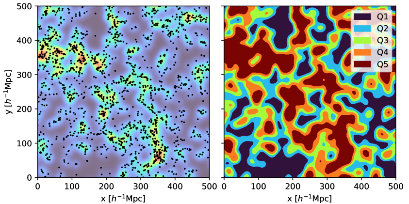
Figure 1: A $500\times 500\ h^{-1}\rm{Mpc}$ cross-section for one of the Quijote fiducial simulation volumes. The slice depth is set to twice the smoothing radius. The left panel shows the projected halo positions in redshift space, and the background colour represents the smoothed density contrast. The right panel shows a map of the associated quantiles. Q1 denotes the most underdense quantile, Q5 denotes the most overdense quantile, and Q2-4 are the intermediate density quantiles.

To help visualize, Fig. 1 shows an example cross-sectional map demonstrating the DSC methodology applied to one of the Quijote fiducial simulation volumes. The existing DSC Fisher analysis [41] used a TopHat filter of radius $R_{\rm s}=20\ h^{-1}\rm{Mpc}$ and performed smoothing in configuration space. We instead follow the convention of more recent DSC analyses [42, 43] and use a Gaussian filter of radius $R_{\rm s}=10\ h^{-1}\rm{Mpc}$, corresponding to an effective TopHat radius (with asymptotically converging window functions in Fourier space as $k\rightarrow 0$) of $R_{\rm s}=10\sqrt{5}\ h^{-1}\rm{Mpc}\sim 22.4\ h^{-1}\rm{Mpc}$, and perform the smoothing in Fourier space to avoid the computationally expensive pair counting procedure. However, instead of fixing the cell size to $5\ h^{-1}\rm{Mpc}$ for the mesh grid, we use a resolution of $N_{\rm mesh}=512$, which, for the given box size, corresponds to a cell size of $\sim 2\ h^{-1}\rm{Mpc}$, helping to reduce additional smoothing effects beyond the Gaussian filter. Existing DSC analyses use the Cloud-In-Cell (CIC) interpolation scheme to paint halos to the mesh, but we instead employ the TSC scheme to further reduce aliasing effects. We do not apply the interlacing technique [55] since it significantly increases computational resources. Lastly, the halo positions are considered in redshift space, which can effectively blur out some of the local density information. The first DSC Fisher analysis [41] showed that reconstruction algorithms can generate a pseudo real-space catalogue to recapture some of the lost information, but also showed that it can introduce additional biases. We choose not to apply reconstruction here and accept the small information loss to avoid unwanted effects and more accurately mimic the conditions of a true galaxy survey.

3.2 Power Spectrum Estimation

The existing DSC analyses [40, 41, 42, 43] work exclusively in configuration space, i.e., using correlation functions as summary statistics. While the power spectrum and correlation function are a Fourier transform pair and encode the same information, there can be significant differences in computational resources and constraining power depending on the scales being probed and the number densities involved. For example, the dominant contribution to computing time for Fourier space is the Fast Fourier Transform (FFT) procedure, which depends only on the resolution of the grid; painting the particles to the mesh is typically a subdominant contribution. On the other hand, configuration space involves a pair counting procedure that is highly sensitive to the number density of the sample. We introduce a DSC Fourier space analysis, which could prove useful for DSC analyses on high-density targets, such as the DESI Bright Galaxy Sample [56]. We leave a more direct comparison between the constraining power and computational resources of both approaches to future work.

To maintain consistency, we use the same grid resolution and resampling and interlacing schemes for the computation of the power spectra as when applying the density-split step to the halo field, except the halo power spectrum where we use CIC interpolation since it is used in other literature [11]. The power spectrum computations were implemented using the publicly available packages pypower and nbodykit. The minimum wavenumber is set to the fundamental mode $k_{\rm min}=2\pi/L$ where $L=1\ h^{-1}\rm{Gpc}$ is the box size, and the maximum wavenumber is set to the Nyquist mode $k_{\rm max}=\pi N_{\rm mesh}/L$, although we limit our analysis to scales $k\leq 0.5\ h\rm{Mpc}^{-1}$ again for consistency with other literature [11, 35]. The bin width is set equal to the minimum wavenumber. We only compute the monopole and quadrupole moments of the power spectra; the hexadecapole also contains non-trivial information in redshift space, but it is too noisy to accurately compute derivatives and contains comparatively little information. The monopole and quadrupole are calculated according to:

$$\hat{P}_{l}(k_{\rm i})=\frac{2l+1}{2N_{\rm i}}\sum_{k_{\rm i,min}\ \leq\ |\vec{k}|\ \leq\ k_{\rm i,max}}L_{l}(\mu)\delta(\vec{k})\delta^{\star}(\vec{k})\,,$$ (3.1)

where $\rm{i}$ denotes the $k$ bin index with $k_{\rm i,max}-k_{\rm i,min}=\Delta k$ being the bin width. $N_{\rm i}$ is the normalization to account for the number of modes in each bin, $\delta(\vec{k})$ are the Fourier modes of the overdensity field and $L_{l}(\mu)$ is the Legendre polynomial of order $l$, where $l=0,2$ correspond to the monopole and quadrupole moments, respectively. We also subtract the $1/\bar{n}$ shot noise contribution for the halo auto power spectra, but not for the quantile auto power spectra for reasons discussed later.

The relevant summary statistics include the quantile auto power spectra, denoted $P^{\rm qq}_{(0,2)}$, the quantile-halo cross power spectra, denoted $P^{\rm qh}_{(0,2)}$, and the halo auto power spectra, denoted $P^{\rm hh}_{(0,2)}$, where $\rm{q}$ denotes the quantile index, $\rm{h}$ denotes the halos and the subscripts $(0,2)$ denote the monopole and quadrupole moments. The previous DSC Fisher analysis [41] focused exclusively on the information content of DSC compared to the standard 2PCF. In our analysis, we also study the joint constraining ability of the DSC power spectra and the halo power spectrum. Fig. 2 shows the monopole and quadrupole of the DSC auto and cross power spectra for the fiducial cosmology.

Given that the query positions – lattice points or randoms – are distributed uniformly before splitting into quantiles, the overdensity fields by definition sum to zero. In other words:

$$\delta_{\rm i}(\vec{x})=-\sum_{\rm j\neq i}\delta_{\rm j}(\vec{x})\,,$$ (3.2)

where $\rm{i}$ and $\rm{j}$ are indices denoting the quantiles. By linearity of expectations, substituting Eq. 3.2 gives the following expression for the quantile-halo cross-correlation:

$$\epsilon_{\rm i,h}(\vec{r})=\left<\delta_{\rm i}(\vec{x})\delta_{\rm h}(\vec{x}-\vec{r})\right>=-\sum_{\rm j\neq i}\left<\delta_{\rm j}(\vec{x})\delta_{\rm h}(\vec{x}-\vec{r})\right>=-\sum_{\rm j\neq i}\epsilon_{\rm j,h}(\vec{r})\,,$$ (3.3)

where $\rm{h}$ denotes the halos. Because any quantile-halo cross-correlation can be expressed as a sum of the remaining quantile-halo cross-correlations, all information from the quantile-halo cross power spectra is encoded in all but one of the available quantiles. We note however that the equivalent argument does not apply for the quantile autocorrelations. To see why, we compute the quantile autocorrelation:

$$\epsilon_{\rm i,i}(\vec{r})=\left<\delta_{\rm i}(\vec{x})\delta_{\rm i}(\vec{x}-\vec{r})\right>=\sum_{\rm j\neq i}\sum_{\rm k\neq i}\left<\delta_{\rm j}(\vec{x})\delta_{\rm k}(\vec{x}-\vec{r})\right>=\sum_{\rm j\neq i}\epsilon_{\rm j,j}(\vec{r})+\sum_{\rm j,k\neq i,j\neq k}\epsilon_{\rm j,k}(\vec{r})\,.$$ (3.4)

Eq. 3.4 shows that any quantile autocorrelation is not merely a sum over the other quantile autocorrelations, but also a sum over the quantile-quantile cross-correlations. The latter are not included under the current implementation of DSC, and thus all quantiles must be included to capture all available information from the quantile auto power spectra. We follow the convention of previous DSC studies [41, 42, 43] and omit the intermediate quantile Q3 while keeping Q1, Q2, Q4, Q5. But instead of omitting the quantile-halo cross and quantile auto power spectra, we merely omit the quantile-halo cross power spectra.

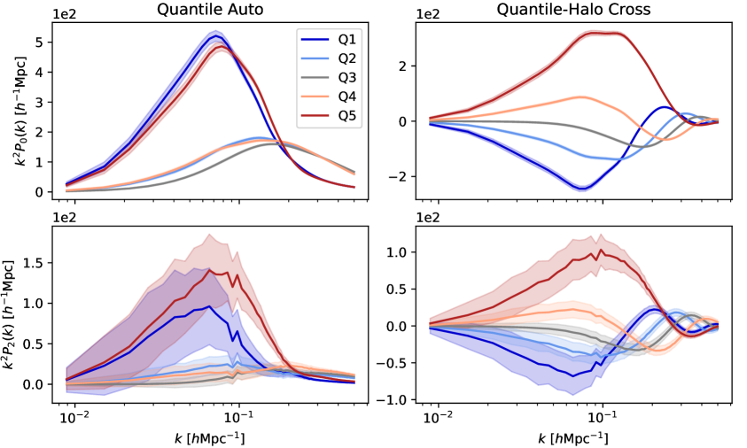
Figure 2: The DSC power spectra for the fiducial cosmology. The solid line is the mean across all realizations, while the shaded region denotes the standard noise for a single realization. The top (bottom) panel denotes the monopole (quadrupole) moment, and the left (right) panel denotes the quantile auto (quantile-halo cross) power spectra.

As introduced earlier, previous applications of DSC [40, 41, 42, 43] have used randomly placed query positions for the quantiles. This approach introduces unnecessary shot noise on small scales. One solution is to populate the volume with a sufficiently large number of randoms such that the additional shot noise is negligible – this is computationally demanding since the average number of randoms per pixel in the grid must be significantly larger than one. Instead, assigning a single query point at the centre of each pixel removes the shot noise introduced when using random query positions, leaving only the shot noise due to the discreteness of the underlying halo field. To test the validity of this alternate approach, appendix A shows a plot comparing the observed power spectra for both approaches – we find close agreement over a broad range of scales. Nevertheless, small differences can be neglected given that an application to data would likely involve an emulator calibrated directly on simulations that will match either convention. In section 4, we discuss the differences in constraining power between these two methods.

3.3 Fisher Information

We employ the Fisher information formalism [57] to quantify the information content of our statistics. Under the simplifying assumption that our data vectors follow multivariate Gaussian distributions and that their covariance matrices do not change significantly with cosmological parameters, the Fisher information matrix simplifies greatly:

$$\boldsymbol{F}_{\rm ij}(\boldsymbol{\theta^{\star}})=\frac{\partial\boldsymbol{\mu}^{T}}{\partial\theta_{\rm i}}\boldsymbol{C}^{-1}\frac{\partial\boldsymbol{\mu}}{\partial\theta_{\rm j}}\bigg{\rvert}_{\boldsymbol{\theta^{\star}}}\,,$$ (3.5)

where $\boldsymbol{\mu}$ is the noise-free data vector as a function of parameter vector $\boldsymbol{\theta}$, $\boldsymbol{C}$ is the covariance matrix of the data vector, and $\rm i,j$ represent the ith and jth indices of the Fisher matrix. These quantities are evaluated around the fiducial model vector $\boldsymbol{\theta}^{\star}$. The Cramér-Rao bound states that the inverse Fisher matrix provides a lower bound on the parameter variances – equality holds if the optimal estimator is utilized:

$$\sigma(\theta_{\rm i})\geq\sqrt{F^{-1}_{\rm ii}}\,.$$ (3.6)

We estimate the derivatives and inverse covariance matrices numerically:

$$\frac{\partial\boldsymbol{\mu}}{\partial\theta_{\rm i}}\bigg{\rvert}_{\boldsymbol{\theta^{\star}}}\approx\frac{\boldsymbol{\bar{\mu}}(\theta^{\star}_{\rm i}+d\theta_{\rm i})-\boldsymbol{\bar{\mu}}(\theta^{\star}_{\rm i}-d\theta_{\rm i})}{2d\theta_{\rm i}}\,,$$ (3.7)

$$\boldsymbol{C}^{-1}\equiv\frac{N_{\text{cov}}-N_{\text{bin}}+N_{\theta}-1}{N_{\text{cov}}-1}\boldsymbol{C^{\prime}}^{-1},\ \ \boldsymbol{C^{\prime}}\equiv\frac{1}{N_{\text{cov}}-1}\sum_{\rm i}^{N_{\text{cov}}}(\boldsymbol{\mu_{\rm i}}^{\star}-\boldsymbol{\bar{\mu}}^{\star})(\boldsymbol{\mu_{\rm i}}^{\star}-\boldsymbol{\bar{\mu}}^{\star})^{T}\,,$$ (3.8)

where $N_{\rm cov}$ is the number of simulations used to compute the covariance matrix, $N_{\rm bin}$ is the number of entries in our data vector, and $N_{\theta}$ is the number of parameters included in the Fisher matrix. $\boldsymbol{\mu_{\rm i}}$ is the ith realization of the data vector and $\boldsymbol{\bar{\mu}}$ is the mean data vector across all realizations, for either the covariance matrix or the numerical derivatives. The $\star$ symbol denotes quantities evaluated at the fiducial cosmology. We apply the correction factor from [58] to debias our estimate of the inverse covariance matrix – similar to [59] but also accounting for the inversion of the Fisher matrix.

4 PNG Fisher Constraints from DSC

Going forward, we shall refer to the following combinations of summary statistics:

$$\vec{d}\equiv\{P^{\rm hh}_{(0,2)}\}\ \ \rightarrow\ \ \text{`Halo'}$$

$$\vec{d}\equiv\{P^{\rm ii}_{(0,2)},P^{\rm jh}_{(0,2)}\},{\rm i}=(1,2,3,4,5),{\rm j}=(1,2,4,5)\ \ \rightarrow\ \ \text{`DSC'}$$

$$\vec{d}\equiv\{P^{\rm hh}_{(0,2)},P^{\rm ii}_{(0,2)},P^{\rm jh}_{(0,2)}\},{\rm i}=(1,2,3,4,5),{\rm j}=(1,2,4,5)\ \ \rightarrow\ \ \text{`Joint'}$$

4.1 Raw Constraints

Fig. 3 shows the constraints for each of the three statistics as a function of the maximum wavenumber. This includes the marginalized (over the PNG shapes, $\Lambda$CDM/mass cut parameters) and unmarginalized constraints. As expected, we observe weakened constraints when marginalizing over other parameters. Fig. 4 presents the corresponding constraints at the maximum wavenumber $k_{\rm max}=0.5\ h\rm{Mpc}^{-1}$, including parameter degeneracies.

Figure 3: Raw, marginalized (solid line) and unmarginalized (dashed line) constraints as a function of maximum fitting wavenumber, for the halo power spectrum, DSC power spectra or joint power spectra.

Figure 4: Contours (1$\sigma$ and 2$\sigma$) for the raw, marginalized constraints at the maximum wavenumber $k_{\rm max}=0.5\ h\rm{Mpc}^{-1}$, for the halo power spectrum, DSC power spectra or joint power spectra.

4.2 Convergence Corrections

We must test the robustness of these results before drawing conclusions. Because we are averaging over a finite number of realizations to compute covariance matrices and derivatives, the estimated constraints will contain noise. Covariance matrices are estimated using 15000 realizations, significantly larger than the 500 realizations used to estimate derivatives. Fig. 5 shows the marginalized constraints as a function of the number of realizations used to estimate covariance matrices and derivatives, normalized to the maximum number of realizations. Each derivative realization is the average of the three LOS directions, while each covariance realization uses just one LOS direction. We observe only percent-level fluctuation with respect to the number of covariance realizations and do not observe any systematic offsets, given that we have applied the corrections to debias our inverse Fisher matrices [58].

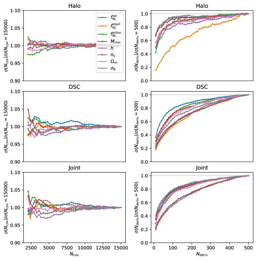
Figure 5: Marginalized constraints normalized to the maximum number of available covariance realizations (left panel) and derivative realizations (right panel).

On the other hand, the noisy derivatives lead to systematically over-optimistic constraints. To understand this intuitively, we provide an analytic proof in Appendix B; we follow the approach motivated by [36] and derive the functional dependence of the constraints on the number of derivative realizations assuming the covariance matrices are known exactly – a reasonable approximation given the large number of realizations compared to the derivatives. The derivation in Appendix B leads to the following dependence:

$$\sigma(\theta_{\rm i})_{\rm corrected}\approx f(\infty)\sigma(\theta_{\rm i})_{\rm raw},\ f(N_{\rm deriv})=\left(\frac{1+C}{1+\frac{500C}{N_{\rm deriv}}}\right)^{1/2}\,,$$ (4.1)

where $C$ is the fitting constant representing the level of convergence and $N_{\rm deriv}$ is the number of derivative realizations. After fitting $C$, we take the limit as $N_{\rm deriv}\rightarrow\infty$ and apply the correction factor $f(\infty)=(1+C)^{1/2}$ to obtain robust estimates. Given that each parameter has a different level of convergence, we fit the expression for each parameter separately. We note that the derived expression only strictly holds in the limit of large $N_{\rm deriv}$, where the central limit theorem applies; we conservatively fit the model only between 100 and 500 derivative realizations to account for this.

The constraints are less strongly converged for the DSC and joint analyses compared to the halo-only analysis. Without applying the proposed corrections above, we would be overestimating the relative improvement from adding DSC functions. Fig. 6 shows the constraints for the DSC and joint fits normalized to the halo-only constraints.

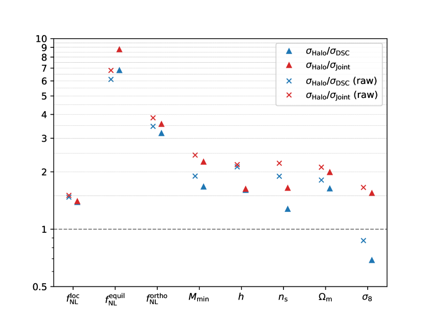
Figure 6: Relative improvement (raw and corrected) for the DSC and joint analyses, compared to the halo-only analysis, across the parameters fitting to the maximum wavenumber of $k_{\rm max}=0.5\ h\rm{Mpc}^{-1}$.

The joint analysis provides factors of $\sim$ 1.4, 8.8, 3.6, 2.3, 1.6, 1.6, 2.0, and 1.5 improvement over the halo-only analysis for parameters $f_{\rm NL}^{\rm loc},f_{\rm NL}^{\rm equil},f_{\rm NL}^{\rm ortho},M_{\rm min},h,n_{s},\Omega_{\rm m},\sigma_{8}$, after applying convergence corrections. Except $f_{\rm NL}^{\rm equil}$, the relative improvements for the DSC and joint analyses from the halo-only analysis are weakened upon applying the convergence correction, confirming the importance of applying these corrections to avoid over-optimistic forecasts. The joint analysis provides improvement over the halo-only analysis for all parameters, while the DSC analysis provides improvement for all parameters except $\sigma_{8}$, highlighting the importance of the joint constraining power of the halo/DSC power spectra.

4.3 Modifications to Hyperparameters

The main results of this paper, along with existing DSC analysis [42, 43], use a fixed Gaussian smoothing radius $R_{\rm s}=10\ h^{-1}\rm{Mpc}$ and number of bins $N_{\rm quantile}=5$. This choice of hyperparameters is not necessarily optimal for extracting maximal information. We additionally test smoothing radii of $R_{\rm s}=7,13\ h^{-1}\rm{Mpc}$, number of density environments $N_{\rm quantile}=3,7$, and switching from randoms (five times the number of halos) to lattice query points in Fig. 7.

For reasons discussed in section 3, we find that switching from random to lattice query positions boosts constraining power for all parameters, matching the limit of a larger number of random points, and reducing the associated shot noise. Except $f_{\rm NL}^{\rm equil}$, all constraints improve as the number of quantiles increases. A larger number of density bins more completely characterizes the non-Gaussian density distribution. At the same time, increasing the number of quantiles also increases the computational expense and the size of the data vector – an important trade-off given that a sufficient number of realizations, relative to the size of the data vector, is needed to obtain a reliable estimate of the covariance matrix. We also observe consistent improvement in the constraints when using smaller smoothing radii – excessively large $R_{\rm s}$ washes out small-scale information. Since halos are a discrete tracer of the matter field, the smoothing radius must be large enough to ensure a sufficient range of densities and prevent it from being highly skewed. The number densities considered in this paper are low compared to upcoming surveys, which will permit smaller smoothing radii before running into this problem. We are also using halos in place of galaxies, which neglects effects arising from the galaxy-halo connection.

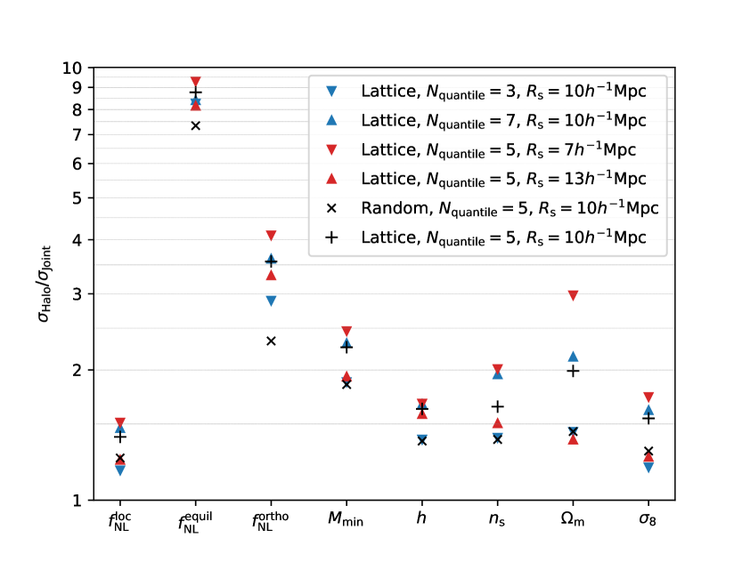
Figure 7: Relative improvement (corrected for derivative convergence) for the joint analysis compared to the halo-only analysis fitting to the maximum wavenumber of $k_{\rm max}=0.5\ h\rm{Mpc}^{-1}$, for variations in the smoothing radius, number of quantiles and query type.

5 Interpretation of Results

5.1 Higher-Order Information

The most significant improvement between the joint DSC/halo analysis and halo-only analysis occurs for PNG of equilateral and orthogonal types (by factors $\sim$ 8.8, 3.6) with less significant improvement (by factors $\lesssim 2.3$) for PNG of local type and the other $\Lambda$CDM/mass cut parameters. This finding closely mirrors a previous study [11], which compared constraints for the joint halo power spectrum/bispectrum with the halo power spectrum. They found that the joint halo power spectrum/bispectrum provided significantly more constraining power compared to the halo power spectrum for equilateral and orthogonal PNG, but more modest enhancements for the remaining parameters. While [11] used a Gaussian process to smooth derivatives to rectify the issue of convergence, and thus the results are not directly comparable to ours, they provide a qualitative framework to compare the information content of the DSC functions with the halo bispectrum. For equilateral and orthogonal PNG, there is a disproportionate amount of information encoded in the halo bispectrum compared to the halo power spectrum. Because DSC performs effectively for these two parameters in particular, we deduce that DSC is an efficient compression of higher-order information.

5.2 Local PNG and Sample Variance Cancellation

In the peak-background split formalism [60, 61], long-wavelength modes modulate the small-scale density field – the effective threshold required for halo formation changes, leading to a (constant) large-scale bias. In the presence of local PNG, the coupling between short and long-wavelength modes leads to an additional scale-dependent bias [8]. The corresponding model for the galaxy-matter cross power spectrum (in real space) takes the following form on linear scales:

$$P_{\rm gm}(k,f_{\rm NL}^{\rm loc})=(b+\Delta b(k)f_{\rm NL}^{\rm loc})P_{\rm mm}(k)=b\left(1+\frac{\Delta b(k)}{b}f_{\rm NL}^{\rm loc}\right)P_{\rm mm}(k)\,,$$ (5.1)

where

$$\Delta b(k)\propto\frac{b_{\Phi}}{k^{2}}\,,$$ (5.2)

in the limit $k\rightarrow 0$ where the transfer function $T(k)\rightarrow 1$, and

$$b_{\Phi}=\frac{\partial\ln{\bar{n}}}{\partial\ln{\sigma_{8}}}\,,$$ (5.3)

measures the response of the galaxy number density to changes in the amplitude of small-scale fluctuations. For multiple tracers of the same underlying matter field with different $b_{\Phi}/b$, we would expect to find sample variance cancellation [10], meaning the error only depends on the shot noise. We might expect that DSC, which generates samples with different large-scale biases, to benefit from sample variance cancellation, in a similar manner to halo catalogues split according to mass. However, we find that DSC provides a smaller improvement for PNG of local type (by factor $\sim 1.4$) compared to the other PNG types. If we restrict to large scales, the information gain comes almost exclusively from degeneracy breaking with other parameters; there is essentially no improvement for the unmarginalized constraints when the maximum wavenumber goes to zero, as shown in Fig. 3.

We can measure the response of the DSC quantiles to $f_{\rm NL}^{\rm loc}$ directly and check for the criteria necessary to achieve sample variance cancellation, by comparing the quantile-matter cross power spectra with different $f_{\rm NL}^{\rm loc}$ . The two variations $f_{\rm NL}^{\rm loc}=\pm 100$ should give opposite responses; we average the two to obtain a more robust estimate instead of relying on either variation exclusively:

$$\frac{\Delta b(k)f_{\rm NL}^{\rm loc}}{b}\equiv\frac{1}{2}\left[{\frac{P_{\rm qm}(k,f_{\rm NL}^{\rm loc})-P_{\rm qm}(k,-f_{\rm NL}^{\rm loc})}{P_{\rm qm}(k,f_{\rm NL}^{\rm loc}=0)}}\right]\,.$$ (5.4)

We can also calculate the (expected) response to $f_{\rm NL}^{\rm loc}$ indirectly from Eq. 5.3, by measuring how the tracer density changes for simulations with different amplitude of small-scale fluctuations $\sigma_{8}^{\pm}=0.834\pm 0.015$ [9]:

$$b_{\Phi}\approx\frac{\ln{(\bar{n}(\sigma_{8}^{+}))}-\ln{(\bar{n}(\sigma_{8}^{-}))}}{\ln{(\sigma_{8}^{+})}-\ln{(\sigma_{8}^{-})}}=\frac{\ln{(\bar{n}(\sigma_{8}^{+})/\bar{n}(\sigma_{8}^{-}))}}{\ln{(\sigma_{8}^{+}/\sigma_{8}^{-})}}\,.$$ (5.5)

For DSC, our ‘tracers’ are represented by pixels in the grid corresponding to each density environment; we need to consider, for variations in $\sigma_{8}$, the change in the number of pixels between fixed thresholds. To choose these thresholds, we average the quantile overdensity boundaries over all fiducial simulations. Combining with a measurement of the linear bias $b$ from the large-scale ratio (averaged on scales $k\leq 0.03\ h\mathrm{Mpc}^{-1}$) of the quantile-matter cross power spectra and the matter power spectrum in real space without local PNG, gives the (expected) ratio $b_{\Phi}/b$ for each quantile.

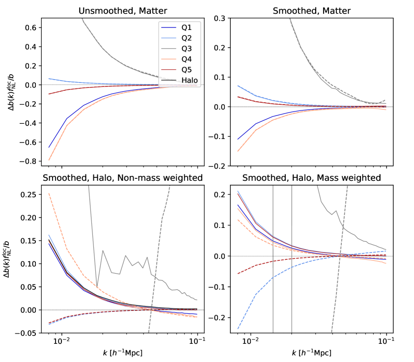
Figure 8: The observed $f_{\rm NL}^{\rm loc}$ responses, in solid lines, for the five DSC quantiles (along with the unsmoothed non-mass-weighted halo field shown in black) according to the unsmoothed matter field, smoothed matter field (Gaussian filter radius $R_{\rm s}=10\ h^{-1}\rm{Mpc}$), smoothed non-mass-weighted halo field (conventional DSC), and smoothed mass-weighted halo field. The dashed lines show the Q1 response re-scaled according to the relative values of $b_{\Phi}/b$ (indirectly computed from Eq. 5.3) for the remaining quantiles.

Fig. 8 shows the observed $f_{\rm NL}^{\rm loc}$ responses when the quantiles are defined by: the unsmoothed matter field, the smoothed matter field (with Gaussian filter radius $R_{\rm s}=10\ h^{-1}\rm{Mpc}$), the smoothed halo number density field (not weighted by mass), and the smoothed halo field weighted by mass, and are compared with the expected responses based on the modelling of Eq. 5.3. The results from the matter field indicate that sample variance cancellation is happening (albeit with less strong differential responses for the smoothed field compared to the unsmoothed field), while those from the halo field indicate it is not. Furthermore, there is strong agreement between the observed and expected responses for quantiles split from the matter field whether the field is smoothed or not, versus strong disagreement when using the smoothed halo field whether weighted by mass or not. The observed responses to $f_{\rm NL}^{\rm loc}$ in the case of the smoothed non-mass-weighted halo field (i.e., DSC as implemented in our Fisher analysis)for Q1, Q2, Q4, Q5 are nearly identical (Q3 appears to have a different response, but the linear bias is nearly zero making the ratio noisy and unreliable), which validates the observed lack of sample variance cancellation from our Fisher forecasts. In contrast, the indirect approach predicts ratios $b_{\Phi}/b\sim$ (0.18, -0.038, -11, 0.31, -0.035) for the five quantiles, which are sufficiently different that we would expect sample variance cancellation to play a role – in theory, the relative amplitudes of the observed $f_{\rm NL}^{\rm loc}$ responses should mirror the relative amplitudes of the ratios $b_{\Phi}/b$, but we see that they do not.

The lack of sample variance cancellation can be understood from the fact that we are deriving the DSC quantiles from a tracer field which is biased and only has a limited range of halo masses; halos below the mass cut $M_{\rm min}=3.2\times 10^{13}\ h^{-1}M_{\odot}$ (lower biased objects) are excluded and the information regarding their $f_{\rm NL}^{\rm loc}$ responses is not present. As the range of halo masses included increases, we expect sample variance cancellation to become increasingly strong, eventually matching what we have found when applied to the (unbiased) smoothed matter field; in the limit that halos of arbitrarily low masses are included, the smoothed mass-weighted halo field should fully characterize the smoothed matter field. In this context, weighting the halos by mass increases the range of $f_{\rm NL}^{\rm loc}$ responses between quantiles, allowing DSC to differentiate between halos of different masses, increasing the information content.

6 Summary

In this paper, we have utilized the Fisher information formalism applied to the Quijote and Quijote-PNG simulations to study the potential for using DSC to constrain PNG of local, equilateral and orthogonal types. After applying the necessary corrections for derivative convergence, we found that a joint DSC/halo power spectrum analysis provided factors of $\sim$ 1.4, 8.8, and 3.6 improvement over a halo power spectrum analysis for PNG of local, equilateral and orthogonal types. These results predict the most significant improvement for PNG of equilateral and orthogonal types, solidifying the hypothesis that DSC is an effective way of probing higher-order information missing from two-point statistics. We observed less significant improvement for PNG of local type due to the absence of significant sample variance cancellation on large scales from scale-dependent bias. We found strong agreement between the observed $f_{\rm NL}^{\rm loc}$ response and the expected response based on the modelling of scale-dependent bias when the quantiles are defined based on either the unsmoothed or smoothed matter overdensity field. Yet, we found strong disagreement when quantiles are defined based on the smoothed halo overdensity field, even when weighted by halo mass – a field generated based on halos within a limited mass range encodes a particular $f_{\rm NL}^{\rm loc}$ response and omits information regarding the $f_{\rm NL}^{\rm loc}$ response to halos outside of the mass range. This is likely to limit the ability of DSC to allow sample variance cancellation for $f_{\rm NL}^{\rm loc}$ when applied to future surveys with a single population of galaxies.

To perform our analysis, we have introduced a Fourier space DSC analysis for the first time and tested a modification of the existing algorithm by using equally spaced lattice query positions instead of randoms, which was found to significantly boost constraining power on small scales. We also briefly studied the impact of varying hyperparameters including the smoothing radius and the number of quantiles, and found that reduced smoothing radius and increased number of quantiles both boosted the information content of the DSC statistics – valuable insights for upcoming applications of DSC to achieve maximal constraining power.

Appendix A Lattice/Random Query Positions

We expect the ensemble mean DSC power spectra using lattice and random query positions to agree closely. Indeed, over the range of wavenumbers probed in this study, we find only percent-level disagreement. However, we expect to see significant differences in noise between these two variations. We expect the noise to agree closely on large scales – where sample variance dominates over shot noise, but for the lattice version to reduce noise on small scales, where the additional shot noise introduced using randoms is eliminated. Fig. 9 confirms both of these predictions by comparing the power spectra for the lattice and random conventions, using five times as many randoms as halos, for one of the DSC quantile autocorrelation monopoles. As shown earlier, this reduction in noise on small scales indeed translates to improved constraining power overall.

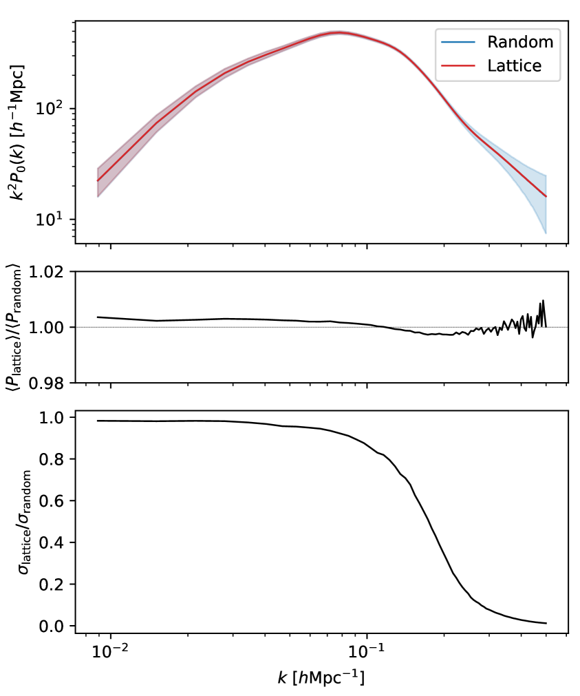
Figure 9: Quantile autocorrelation monopole for Q5 (the most overdense quantile) when using lattice or randomly positioned query positions (five times the number of halos). The top panel shows the mean power spectra and the standard noise for both methods. The middle panel shows the ratio of the mean power spectra for both versions. The lower panel shows the ratio of the standard noise between the lattice and random versions.

Appendix B Derivative Convergence Correction

To derive the analytic expression for the derivative convergence, we first make several simplifying assumptions. We assume that we only have one parameter being varied and one entry in our data vector, and thus the covariance matrix is replaced by the variance of the data entry. The estimator for the Fisher matrix is given by:

$$\hat{F}=\frac{1}{\sigma_{\mu}^{2}}\left(\frac{\partial{\hat{\bar{\mu}}}}{\partial\theta}\right)^{2}\,.$$

Since the number of covariance realizations is much larger than the number of derivative realizations, we also assume the noise in the covariance matrix is negligible compared to the derivatives, and thus we assume the variance here is a constant. We take the expectation value of the Fisher information:

$$\left<\hat{F}\right>=\frac{1}{\sigma_{\mu}^{2}}\left<\left(\frac{\partial\hat{\bar{\mu}}}{\partial\theta}\right)^{2}\right>=\frac{1}{\sigma_{\mu}^{2}}\left[\left(\frac{\partial\bar{\mu}}{\partial\theta}\right)^{2}+\text{Var}\left(\frac{\partial\hat{\bar{\mu}}}{\partial\theta}\right)\right]=F+\frac{1}{\sigma_{\mu}^{2}}\text{Var}\left(\frac{\partial\hat{\bar{\mu}}}{\partial\theta}\right)\,.$$

Since

$$\hat{\bar{\mu}}=\frac{1}{N_{\text{deriv}}}\sum_{\rm i}^{N_{\text{deriv}}}\mu_{\rm i}\,,$$

is the average across many derivative realizations, we can apply the central limit theorem to obtain the variance of the mean in terms of the variance of a single realization:

$$\left<\hat{F}\right>=F+\frac{1}{\sigma_{\mu}^{2}N_{\text{deriv}}}\text{Var}\left(\frac{\partial\hat{\mu}_{\rm i}}{\partial\theta}\right)=F\left(1+\frac{1}{\sigma_{\mu}^{2}N_{\text{deriv}}F}\text{Var}\left(\frac{\partial\hat{\mu}_{\rm i}}{\partial\theta}\right)\right)\,.$$

We can absorb the terms $\sigma_{\mu}^{2}$, $F$ and $\text{Var}\left(\frac{\partial\hat{\mu}_{\rm i}}{\partial\theta}\right)$ into a single constant since we are fitting a model to the observed convergence. We therefore have:

$$\left<\hat{F}\right>^{-1}=F^{-1}\left(1+\frac{500C}{N_{\text{deriv}}}\right)^{-1}\,,$$

where

$$C\equiv\frac{\text{Var}\left(\frac{\partial\hat{\mu}_{\rm i}}{\partial\theta}\right)}{500\sigma_{\mu}^{2}F}\,.$$

Next, we substitute the parameter errors based on the Cramér-Rao bound:

$$\sigma_{\theta}^{2}(N_{\text{deriv}})=\sigma_{\theta}^{2}\left(1+\frac{500C}{N_{\text{deriv}}}\right)^{-1}\,.$$

Now, we normalize to the maximum number of realizations and take the square root:

$$\frac{\sigma_{\theta}(N_{\text{deriv}})}{\sigma_{\theta}(N_{\text{deriv}}=500)}=\left(\frac{1+C}{1+\frac{500C}{N_{\text{deriv}}}}\right)^{1/2}\,.$$

Although the simplifying assumptions we have made here do not hold under a more general Fisher analysis with multiple parameters and entries in the data vector, we expect the same dependence on the number of realizations to hold and we have verified that the functional form provides strong qualitative agreement with the shape of the derivative convergences.

References

- [1] A.. Guth and S.-Y. Pi “Fluctuations in the New Inflationary Universe” In Physical Review Letters 49.15, 1982, pp. 1110–1113 DOI: 10.1103/PhysRevLett.49.1110
- [2] S.. Hawking “The development of irregularities in a single bubble inflationary universe” In Physics Letters B 115.4, 1982, pp. 295–297 DOI: 10.1016/0370-2693(82)90373-2
- [3] Ana Achúcarro et al. “Inflation: Theory and Observations” In arXiv e-prints, 2022, pp. arXiv:2203.08128 DOI: 10.48550/arXiv.2203.08128
- [4] Planck Collaboration et al. “Planck 2018 results. IX. Constraints on primordial non-Gaussianity” In Astronomy and Astrophysics 641, 2020, pp. A9 DOI: 10.1051/0004-6361/201935891
- [5] V. Desjacques and U. Seljak “Primordial non-Gaussianity from the large-scale structure” In Classical and Quantum Gravity 27.12, 2010, pp. 124011 DOI: 10.1088/0264-9381/27/12/124011
- [6] DESI Collaboration et al. “The DESI Experiment Part I: Science,Targeting, and Survey Design” In arXiv e-prints, 2016, pp. arXiv:1611.00036 DOI: 10.48550/arXiv.1611.00036
- [7] R. Laureijs et al. “Euclid Definition Study Report” In arXiv e-prints, 2011, pp. arXiv:1110.3193 DOI: 10.48550/arXiv.1110.3193
- [8] Neal Dalal, Olivier Doré, Dragan Huterer and Alexander Shirokov “Imprints of primordial non-Gaussianities on large-scale structure: Scale-dependent bias and abundance of virialized objects” In Phys. Rev. D 77 American Physical Society, 2008, pp. 123514 DOI: 10.1103/PhysRevD.77.123514
- [9] Emanuele Castorina, Yu Feng, Uroš Seljak and Francisco Villaescusa-Navarro “Primordial Non-Gaussianities and Zero-Bias Tracers of the Large-Scale Structure” In Physical Review Letters 121.10, 2018, pp. 101301 DOI: 10.1103/PhysRevLett.121.101301
- [10] Uroš Seljak “Extracting Primordial Non-Gaussianity without Cosmic Variance” In Physical Review Letters 102.2, 2009, pp. 021302 DOI: 10.1103/PhysRevLett.102.021302
- [11] William R. Coulton et al. “Quijote-PNG: The Information Content of the Halo Power Spectrum and Bispectrum” In Astrophysical Journal 943.2, 2023, pp. 178 DOI: 10.3847/1538-4357/aca7c1
- [12] Emiliano Sefusatti, Martín Crocce, Sebastián Pueblas and Román Scoccimarro “Cosmology and the bispectrum” In Physical Review D 74.2, 2006, pp. 023522 DOI: 10.1103/PhysRevD.74.023522
- [13] Héctor Gil-Marín et al. “The clustering of galaxies in the SDSS-III Baryon Oscillation Spectroscopic Survey: RSD measurement from the LOS-dependent power spectrum of DR12 BOSS galaxies” In Monthly Notices of the Royal Astronomical Society 460.4, 2016, pp. 4188–4209 DOI: 10.1093/mnras/stw1096
- [14] Zachary Slepian and Daniel J. Eisenstein “Modelling the large-scale redshift-space 3-point correlation function of galaxies” In Monthly Notices of the Royal Astronomical Society 469.2, 2017, pp. 2059–2076 DOI: 10.1093/mnras/stx490
- [15] Oliver H.. Philcox, Jiamin Hou and Zachary Slepian “A First Detection of the Connected 4-Point Correlation Function of Galaxies Using the BOSS CMASS Sample” In arXiv e-prints, 2021, pp. arXiv:2108.01670 DOI: 10.48550/arXiv.2108.01670
- [16] István Szapudi and Jun Pan “On Recovering the Nonlinear Bias Function from Counts-in-Cells Measurements” In Astrophysical Journal 602.1, 2004, pp. 26–37 DOI: 10.1086/380920
- [17] Cora Uhlemann et al. “Fisher for complements: extracting cosmology and neutrino mass from the counts-in-cells PDF” In Monthly Notices of the Royal Astronomical Society 495.4 Oxford University Press (OUP), 2020, pp. 4006–4027 DOI: 10.1093/mnras/staa1155
- [18] Mark C. Neyrinck, István Szapudi and Alexander S. Szalay “Rejuvenating the Matter Power Spectrum: Restoring Information with a Logarithmic Density Mapping” In Astrophysical Journal, Letters 698.2, 2009, pp. L90–L93 DOI: 10.1088/0004-637X/698/2/L90
- [19] Yuting Wang et al. “Extracting high-order cosmological information in galaxy surveys with power spectra” In Communications Physics 7.1, 2024, pp. 130 DOI: 10.1038/s42005-024-01624-7
- [20] Guilhem Lavaux and Benjamin D. Wandelt “Precision Cosmography with Stacked Voids” In Astrophysical Journal 754.2, 2012, pp. 109 DOI: 10.1088/0004-637X/754/2/109
- [21] Seshadri Nadathur et al. “The completed SDSS-IV extended baryon oscillation spectroscopic survey: geometry and growth from the anisotropic void-galaxy correlation function in the luminous red galaxy sample” In Monthly Notices of the Royal Astronomical Society 499.3, 2020, pp. 4140–4157 DOI: 10.1093/mnras/staa3074
- [22] Sofia Contarini et al. “Cosmological Constraints from the BOSS DR12 Void Size Function” In Astrophysical Journal 953.1, 2023, pp. 46 DOI: 10.3847/1538-4357/acde54
- [23] Tristan S. Fraser et al. “Modelling the BOSS void-galaxy cross-correlation function using a neural-network emulator” In arXiv e-prints, 2024, pp. arXiv:2407.03221 DOI: 10.48550/arXiv.2407.03221
- [24] C. Wagner, F. Schmidt, C.-T. Chiang and E. Komatsu “Separate universe simulations.” In Monthly Notices of the Royal Astronomical Society 448, 2015, pp. L11–L15 DOI: 10.1093/mnrasl/slu187
- [25] Chi-Ting Chiang et al. “Position-dependent correlation function from the SDSS-III Baryon Oscillation Spectroscopic Survey Data Release 10 CMASS sample” In Journal of Cosmology and Astroparticle Physics 2015.9, 2015, pp. 028–028 DOI: 10.1088/1475-7516/2015/09/028
- [26] Martin White “A marked correlation function for constraining modified gravity models” In Journal of Cosmology and Astroparticle Physics 2016.11 IOP Publishing, 2016, pp. 057–057 DOI: 10.1088/1475-7516/2016/11/057
- [27] Elena Massara and Ravi K. Sheth “Density and velocity profiles around cosmic voids” In arXiv e-prints, 2018, pp. arXiv:1811.03132 DOI: 10.48550/arXiv.1811.03132
- [28] Arka Banerjee and Tom Abel “Nearest neighbour distributions: New statistical measures for cosmological clustering” In Monthly Notices of the Royal Astronomical Society 500.4, 2021, pp. 5479–5499 DOI: 10.1093/mnras/staa3604
- [29] Sihan Yuan, Tom Abel and Risa H. Wechsler “Robust cosmological inference from non-linear scales with k-th nearest neighbour statistics” In Monthly Notices of the Royal Astronomical Society 527.2, 2024, pp. 1993–2009 DOI: 10.1093/mnras/stad3359
- [30] J. Schmalzing, M. Kerscher and T. Buchert “Minkowski Functionals in Cosmology” In Dark Matter in the Universe, 1996, pp. 281 DOI: 10.48550/arXiv.astro-ph/9508154
- [31] Martha Lippich and Ariel G. Sánchez “MEDUSA: Minkowski functionals estimated from Delaunay tessellations of the three-dimensional large-scale structure” In Monthly Notices of the Royal Astronomical Society 508.3, 2021, pp. 3771–3784 DOI: 10.1093/mnras/stab2820
- [32] Stephen Appleby et al. “Minkowski Functionals of SDSS-III BOSS: Hints of Possible Anisotropy in the Density Field?” In Astrophysical Journal 928.2, 2022, pp. 108 DOI: 10.3847/1538-4357/ac562a
- [33] Wei Liu, Aoxiang Jiang and Wenjuan Fang “Probing massive neutrinos with the Minkowski functionals of the galaxy distribution” In Journal of Cosmology and Astroparticle Physics 2023.9, 2023, pp. 037 DOI: 10.1088/1475-7516/2023/09/037
- [34] Georgios Valogiannis and Cora Dvorkin “Towards an optimal estimation of cosmological parameters with the wavelet scattering transform” In Physical Review D 105.10, 2022, pp. 103534 DOI: 10.1103/PhysRevD.105.103534
- [35] Matteo Peron, Gabriel Jung, Michele Liguori and Massimo Pietroni “Constraining Primordial Non-Gaussianity from Large Scale Structure with the Wavelet Scattering Transform” In arXiv e-prints, 2024, pp. arXiv:2403.17657 DOI: 10.48550/arXiv.2403.17657
- [36] Jiamin Hou, Azadeh Moradinezhad Dizgah, ChangHoon Hahn and Elena Massara “Cosmological information in skew spectra of biased tracers in redshift space” In Journal of Cosmology and Astroparticle Physics 2023.3, 2023, pp. 045 DOI: 10.1088/1475-7516/2023/03/045
- [37] Krishna Naidoo, Elena Massara and Ofer Lahav “Cosmology and neutrino mass with the minimum spanning tree” In Monthly Notices of the Royal Astronomical Society 513.3, 2022, pp. 3596–3609 DOI: 10.1093/mnras/stac1138
- [38] Junsup Shim et al. “Probing cosmology via the clustering of critical points” In Monthly Notices of the Royal Astronomical Society 528.2, 2024, pp. 1604–1614 DOI: 10.1093/mnras/stae151
- [39] Beyond-2pt Collaboration et al. “A Parameter-Masked Mock Data Challenge for Beyond-Two-Point Galaxy Clustering Statistics” In arXiv e-prints, 2024, pp. arXiv:2405.02252 DOI: 10.48550/arXiv.2405.02252
- [40] Enrique Paillas, Yan-Chuan Cai, Nelson Padilla and Ariel G. Sánchez “Redshift-space distortions with split densities” In Monthly Notices of the Royal Astronomical Society 505.4, 2021, pp. 5731–5752 DOI: 10.1093/mnras/stab1654
- [41] Enrique Paillas et al. “Constraining CDM with density-split clustering” In Monthly Notices of the Royal Astronomical Society 522.1, 2023, pp. 606–625 DOI: 10.1093/mnras/stad1017
- [42] Enrique Paillas et al. “Cosmological constraints from density-split clustering in the BOSS CMASS galaxy sample” In Monthly Notices of the Royal Astronomical Society 531.1, 2024, pp. 898–918 DOI: 10.1093/mnras/stae1118
- [43] Carolina Cuesta-Lazaro et al. “SUNBIRD: a simulation-based model for full-shape density-split clustering” In Monthly Notices of the Royal Astronomical Society 531.3, 2024, pp. 3336–3356 DOI: 10.1093/mnras/stae1234
- [44] D. Gruen et al. “Density split statistics: Cosmological constraints from counts and lensing in cells in DES Y1 and SDSS data” In Physical Review D 98.2, 2018, pp. 023507 DOI: 10.1103/PhysRevD.98.023507
- [45] O. Friedrich et al. “Density split statistics: Joint model of counts and lensing in cells” In Physical Review D 98.2, 2018, pp. 023508 DOI: 10.1103/PhysRevD.98.023508
- [46] Pierre A. Burger et al. “KiDS-1000 cosmology: Constraints from density split statistics” In Astronomy and Astrophysics 669, 2023, pp. A69 DOI: 10.1051/0004-6361/202244673
- [47] Ummi Abbas and Ravi K. Sheth “Strong clustering of underdense regions and the environmental dependence of clustering from Gaussian initial conditions” In Monthly Notices of the Royal Astronomical Society 378.2, 2007, pp. 641–648 DOI: 10.1111/j.1365-2966.2007.11806.x
- [48] Jeremy L. Tinker “Redshift-space distortions with the halo occupation distribution - II. Analytic model” In Monthly Notices of the Royal Astronomical Society 374.2, 2007, pp. 477–492 DOI: 10.1111/j.1365-2966.2006.11157.x
- [49] Adrian E. Bayer et al. “Detecting Neutrino Mass by Combining Matter Clustering, Halos, and Voids” In Astrophysical Journal 919.1, 2021, pp. 24 DOI: 10.3847/1538-4357/ac0e91
- [50] Tony Bonnaire, Nabila Aghanim, Joseph Kuruvilla and Aurélien Decelle “Cosmology with cosmic web environments. I. Real-space power spectra” In Astronomy and Astrophysics 661, 2022, pp. A146 DOI: 10.1051/0004-6361/202142852
- [51] Tony Bonnaire, Joseph Kuruvilla, Nabila Aghanim and Aurélien Decelle “Cosmology with cosmic web environments. II. Redshift-space auto and cross-power spectra” In Astronomy and Astrophysics 674, 2023, pp. A150 DOI: 10.1051/0004-6361/202245626
- [52] Francisco Villaescusa-Navarro et al. “The Quijote Simulations” In Astrophysical Journal, Supplement 250.1, 2020, pp. 2 DOI: 10.3847/1538-4365/ab9d82
- [53] M. Davis, G. Efstathiou, C.. Frenk and S… White “The evolution of large-scale structure in a universe dominated by cold dark matter” In Astrophysical Journal 292, 1985, pp. 371–394 DOI: 10.1086/163168
- [54] William R. Coulton et al. “Quijote-PNG: Simulations of Primordial Non-Gaussianity and the Information Content of the Matter Field Power Spectrum and Bispectrum” In Astrophysical Journal 943.1, 2023, pp. 64 DOI: 10.3847/1538-4357/aca8a7
- [55] E. Sefusatti, M. Crocce, R. Scoccimarro and H… Couchman “Accurate estimators of correlation functions in Fourier space” In Monthly Notices of the Royal Astronomical Society 460.4, 2016, pp. 3624–3636 DOI: 10.1093/mnras/stw1229
- [56] ChangHoon Hahn et al. “The DESI Bright Galaxy Survey: Final Target Selection, Design, and Validation” In Astronomical Journal 165.6, 2023, pp. 253 DOI: 10.3847/1538-3881/accff8
- [57] R.. Fisher “The Logic of Inductive Inference” In Journal of the Royal Statistical Society 98.1, 2018, pp. 39–54 DOI: 10.1111/j.2397-2335.1935.tb04208.x
- [58] Will J. Percival, Oliver Friedrich, Elena Sellentin and Alan Heavens “Matching Bayesian and frequentist coverage probabilities when using an approximate data covariance matrix” In Monthly Notices of the Royal Astronomical Society 510.3, 2022, pp. 3207–3221 DOI: 10.1093/mnras/stab3540
- [59] J. Hartlap, P. Simon and P. Schneider “Why your model parameter confidences might be too optimistic. Unbiased estimation of the inverse covariance matrix” In Astronomy and Astrophysics 464.1, 2007, pp. 399–404 DOI: 10.1051/0004-6361:20066170
- [60] Shaun Cole and Nick Kaiser “Biased clustering in the cold dark matter cosmogony.” In Monthly Notices of the Royal Astronomical Society 237, 1989, pp. 1127–1146 DOI: 10.1093/mnras/237.4.1127
- [61] Ravi K. Sheth and Giuseppe Tormen “Large-scale bias and the peak background split” In Monthly Notices of the Royal Astronomical Society 308.1 Oxford University Press (OUP), 1999, pp. 119–126 DOI: 10.1046/j.1365-8711.1999.02692.x