Pattern Localisation in Swift-Hohenberg via Slowly Varying Spatial Heterogeneity

Abstract

Theories of localised pattern formation are important to understand a broad range of natural patterns, but are less well-understood than more established mechanisms of domain-filling pattern formation. Here, we extend recent work on pattern localisation via slow spatial heterogeneity in reaction-diffusion systems to the Swift-Hohenberg equation. We use a WKB asymptotic approach to show that, in the limit of a large domain and slowly varying heterogeneity, conditions for Turing-type linear instability localise in a simple way, with the spatial variable playing the role of a parameter. For nonlinearities locally corresponding to supercritical bifurcations in the spatially homogeneous system, this analysis asymptotically predicts regions where patterned states are confined, which we confirm numerically. We resolve the inner region of this asymptotic approach, finding excellent agreement with the tails of these confined pattern regions. In the locally subcritical case, however, this theory is insufficient to fully predict such confined regions, and so we propose an approach based on numerical continuation of a local homogeneous analog system. Pattern localisation in the heterogeneous system can then be determined based on the Maxwell point of this system, with the spatial variable parameterizing this point. We compare this theory of localisation via spatial heterogeneity to localised patterns arising from homoclinic snaking, and suggest a way to distinguish between different localisation mechanisms in natural systems based on how these structures decay to the background state (i.e. how their tails decay). We also explore cases where both of these local theories of pattern formation fail to capture the interaction between spatial heterogeneity and underlying pattern-forming mechanisms, suggesting that more work needs to be done to fully disentangle exogenous and intrinsic heterogeneity.

35B36, 35B32

1 Introduction

A contemporary question in many areas of science is to understand the origin of natural spatial structures [43, 35, 40, 31]. In particular, given an observed spatial distribution (henceforth, pattern), it is relevant to understand if the mechanisms underlying its formation are due to intrinsic self-organisation (e.g. from Turing-like pattern forming mechanisms [46, 31]) or to exogenous factors, such as environmental heterogeneity in the context of ecosystems or developing tissue structures. Examples include in plant-root initiation [8, 9], hierarchical patterning in embryology [42, 37], as well as in vegetation patterning and neuroscience [41]. Questions of intrinsic or extrinsic factors underlying pattern formation become even more intricate with regards to localised pattern formation, whereby oscillatory spatial structures are confined to distinct spatial regions, falling away to background states that would not be classified as structured or patterned regions [26]. In this paper, we consider a spatially-heterogeneous Swift-Hohenberg equation as a prototype model for understanding the interplay between nonlinearity and spatial heterogeneity in giving rise to localised patterns.

Spatially heterogeneous systems are likely more realistic models than their simpler homogeneous counterparts, particularly for embryological and ecological phenomena. Turing himself was aware of this, noting that most biological structures likely “evolve from one pattern into another, rather than from homogeneity into a pattern” [46]. A major reason for emphasizing simpler homogeneous models is due to how much more difficult even relatively simple techniques, such as linear stability analysis, become in the heterogeneous case [33, 31]. Nevertheless, there is a growing body of work exploring such heterogeneous systems numerically [6, 2, 38, 39, 25, 32, 49] and in asymptotic regimes [24, 27, 33, 19], among other approaches [5, 44, 48, 13]. Spatial and spatiotemporal heterogeneity has been used to design Turing spaces matching complex prepatterns and pattern-forming regions [53], as well as in orienting stripes [21, 16].

Recent work [33, 19, 17, 32, 41] has explored how bifurcations seen in spatially homogeneous settings play out in spatially heterogeneous systems, where the heterogeneity passes through values around these bifurcation points. The qualitative features here, in the case of Turing-type bifurcations, are a localisation of classical Turing conditions leading to a type of confined pattern formation distinct from the localisation observed in spatially homogeneous systems. An important lesson arising from this work is that a naive local theory of heterogeneity (essentially treating spatial variables as parameters) can successfully explain observed behaviours in heterogeneous systems in some cases (e.g. [33, 19], and even for spatiotemporally forced systems [17]), but critically fails to explain some emergent dynamics (e.g. [32, 41]). Clarifying when the intuitive local picture accurately captures the dynamics, and when it does not, is the main goal of this paper, with a secondary aim of investigating how the decay of localised pattern back to baseline (i.e. the patterned solution’s tail) may indicate the underlying pattern formation mechanism.

To address these issues, we will study a particularly simple model of slowly varying heterogeneity. Namely, we consider a heterogeneous Swift-Hohenberg equation of the form,

(1) $$\frac{\partial u}{\partial t}=r(x)u-\left(1+\varepsilon^{2}\frac{\partial^{2}}{\partial x^{2}}\right)^{2}u+N(u),\quad\quad\quad x\in[0,1],$$

where we assume that $N(0)=N_{u}(0)=0$ and $0<\varepsilon\ll 1$. To represent a closed system so that any pattern formation is an emergent property of the system rather than due to external forcing at the boundary, the associated boundary conditions are taken to be the generalised Neumann conditions

(2) $$u_{x}(t,0)=u_{xxx}(t,0)=0=u_{x}(t,1)=u_{xxx}(t,1).$$

This model has the corresponding energy functional,

(3) $$E(u)=-\int_{0}^{1}\frac{1}{2}\left(r(x)u^{2}-\left(u+\varepsilon^{2}\frac{\partial^{2}u}{\partial x^{2}}\right)^{2}\right)+F(u)dx,\quad F(u)=\int_{0}^{u}N(v)dv,$$

from which we see that all stable states for asymptotically large times must be stationary (ruling out heterogeneity-induced spatiotemporal dynamics, as in [39, 32, 27]). We assume that all functions are sufficiently smooth, and in particular that $|r^{\prime}(x)|=o(1/\varepsilon)$, i.e. the heterogeneity varies slowly. This model is essentially equivalent to a spatial dynamics formulation (as in [3] and elsewhere) with a slowly varying heterogeneity relative to any other length scales in the problem. We will also consider a homogeneous analog of Eq. 1 given by,

(4) $$\frac{\partial u}{\partial t}=r_{h}u-\left(1+\varepsilon^{2}\frac{\partial^{2}}{\partial x^{2}}\right)^{2}u+N(u),\quad\quad\quad x\in[0,1],$$

assuming the same boundary conditions Eq. 2. This model also has an energy functional of the form of Eq. 3. Our goal is then to understand when the dynamics of Eq. 1 can be understood by looking at the dynamics of Eq. 4 with $r(x)=r_{h}$ locally in $x$ (i.e. when a ‘quasi-static’ approach in space can be justified).

We illustrate this in Fig. 1, showing a long-time solution of the homogeneous system in panel (a), and a corresponding heterogeneous system in panel (b) for the same value of $\varepsilon$, with panels (c) and (d) showing simulations with smaller values of $\varepsilon$. The red lines correspond to $r(x)=0$, and hence to where a naive local theory would predict pattern confinement. Following asymptotic analyses of heterogeneous reaction-diffusion [33] and reaction-cross-diffusion systems [19], we will justify this intuitive picture in the limit of small $\varepsilon$ by showing that the linear stability problem leads to locally supported solutions within these regions. We also fill an important gap in these papers by carrying out a boundary-layer analysis at the bifurcation crossing, to approximate how the tails of the solutions behave near points where $r(x)=0$. Importantly, these ideas from linear theory will be shown to only work when the local picture is supercritical. In the locally subcritical case, we will develop an alternative prediction for the confinement region based on the idea of a local Maxwell point of the energy functional Eq. 3. We will also numerically explore cases where neither approach successfully predicts heterogeneity-induced pattern localisation, raising important questions about how to understand such systems in general. Overall these ideas will give a partial answer to what we can learn about a system’s underlying patterning mechanisms based on observed patterned states.

We remark that the form of localisation from supercritical bifurcations in the presence of heterogeneity differs from that of localised solutions arising in spatially homogeneous models, such as Eq. 4, due to homoclinic snaking [52, 12, 3, 14, 26, 1]. We give examples of the latter type of solution in Fig. 2, where we have simulated the homogeneous model using initial data constructed from the simulation in Fig. 1(a) by setting some parts of this solution to zero, and then evolving forward in time. This leads to a fundamentally different kind of localized solution. We remark that there are several ways to numerically find such states once a good parameter regime is known, such as via numerical continuation [47]. There are several differences to the simulations shown in Fig. 1 with these localised states, both in their qualitative properties (e.g. sharper tails, and a degree of translation invariance away from the boundaries) and in the details of the nonlinearities in determining their existence (e.g. they generally arise in the bistable regime of a subcritical Turing bifurcation). In particular, the tails in the case of heterogeneity across a supercritical bifurcation appear algebraic, while the localised solutions arising from snaking are exponential. Motivated by these distinctions, we will return to compare and contrast such localised states with those arising in spatially heterogeneous models later.

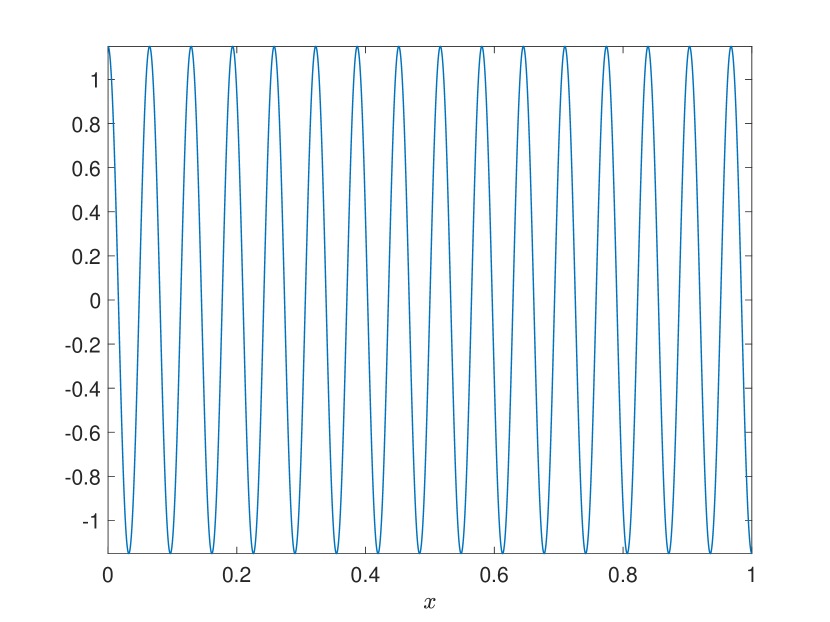
(a) $r=1$, $\varepsilon=0.01$

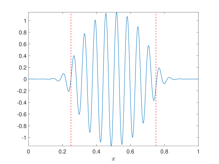
(b) $r=-\cos(2\pi x)$, $\varepsilon=0.01$

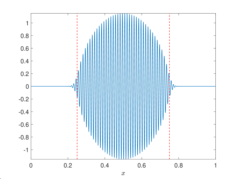
(c) $r=-\cos(2\pi x)$, $\varepsilon=0.002$

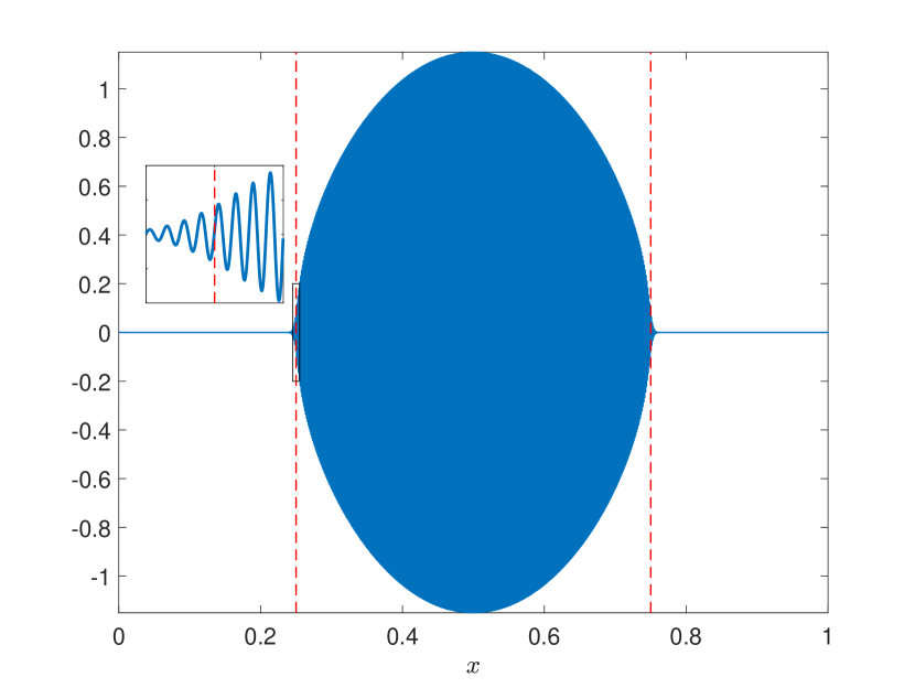
(d) $r=-\cos(2\pi x)$, $\varepsilon=0.0002$

Figure 1: Solutions $u(x)$ of Eq. 1 (blue solid curves) with the cubic nonlinearity $N(u)=-u^{3}$ for varying $r(x)$ and $\varepsilon$. Panel (a) is the homogeneous case corresponding to Eq. 4, whereas (b)-(d) are spatially heterogeneous, with dashed red vertical lines indicating at $x=0.25,0.75$ where $r(x)=0$, and hence where a naive theory would predict patterning confinement. The inset in (d) shows the pattern transition region over $x\in[0.245,0.255]$. Simulation details can be found in Appendix B.

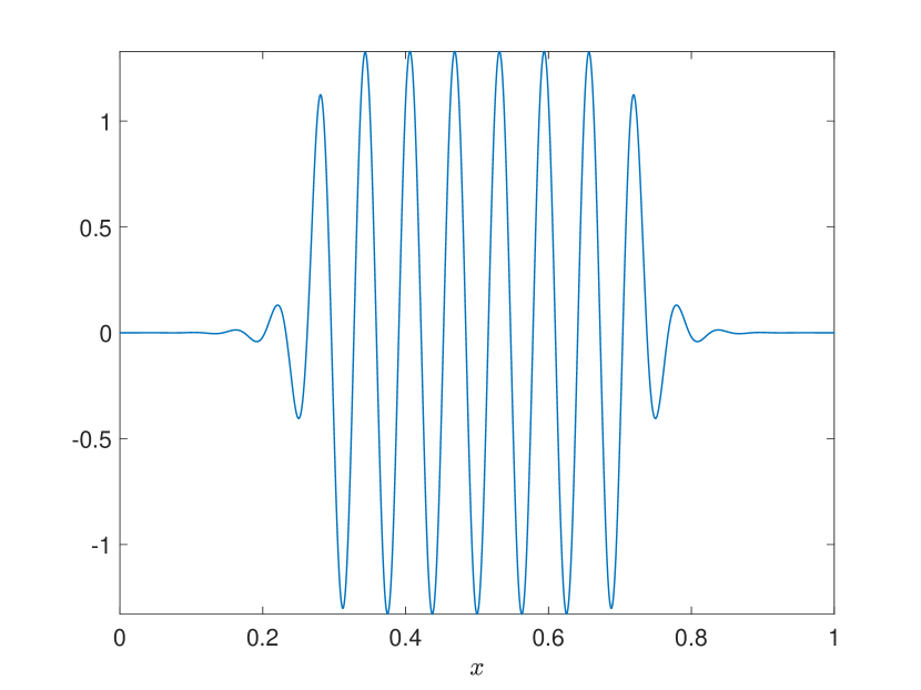
(a) $\varepsilon=0.01$

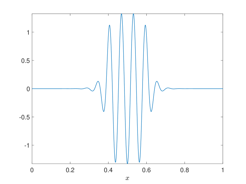
(b) $\varepsilon=0.01$

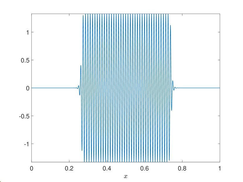
(c) $\varepsilon=0.002$

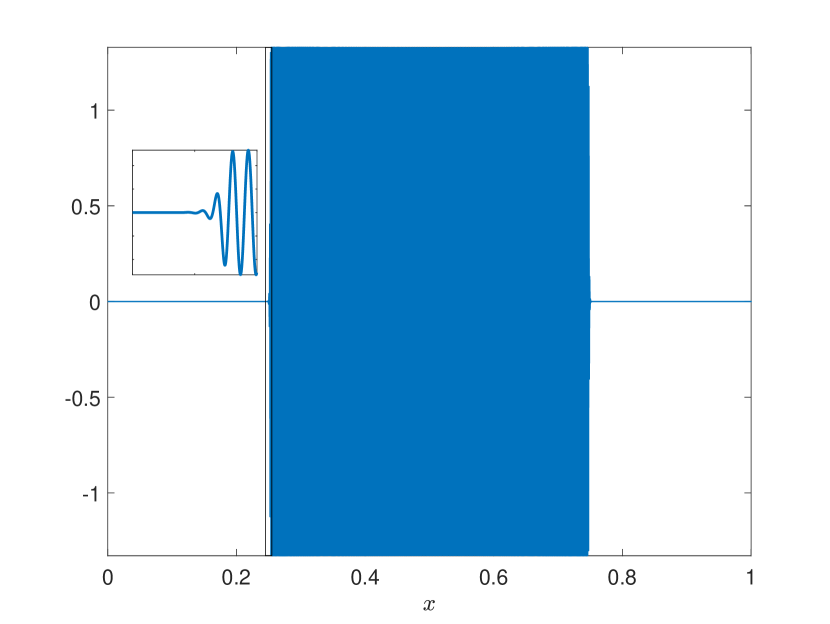
(d) $\varepsilon=0.0002$

Figure 2: Solutions $u(x)$ of Eq. 4 (blue solid curves) with the quadratic-quintic nonlinearity $N(u)=2u^{3}-u^{5}$ with $r_{h}=-0.7$. Different initial data were used for the simulation as described in the text. The inset in (d) shows the pattern transition region over $x\in[0.245,0.255]$. Note that the $x$ axis in the inset of (d) is the same as in Fig. 1(d), but the $y$ axis here is much larger. Simulation details can be found in Appendix B.

The rest of this paper is organized as follows. In Section 2 we develop a linear stability theory in the limit of small $\varepsilon$ using WKB theory. This gives an exact analogy between pattern-forming conditions in the heterogeneous model and such conditions in a local homogeneous variant corresponding to pattern confinement for $r(x)>0$. In Section 3, we resolve the boundary layer around the bifurcation points where the leading-order outer WKB solutions are singular, showing how solution envelopes are predicted to decay according to the linear theory. In Section 4, we demonstrate that the theory generically fails to predict confinement regions when the bifurcation is locally subcritical, for which we propose an alternative prediction based on Maxwell points of a local analog system, which is only successful for some choices of parameters and nonlinearities. Finally we discuss these results in Section 5, explaining further directions emerging from this work, and highlighting important barriers to classical bifurcation-theoretic paradigms.

2 Localisation of Turing instabilities

We now study the canonical Turing instability for this system about the homogeneous steady state $u=0$, leading to a linear problem of the form Eq. 1 with $N(u)=0$. A Turing instability then requires linear stability for homogeneous perturbations, but an instability for a spatially varying perturbation. While such bifurcations are readily studied for constant coefficient systems, the fact that we have $r(x)$ as a function of $x$ entails that the linear stability theory is more involved, as naive expansions in terms of trigonometric eigenfunctions would not diagonalize the linear operator, and hence one cannot study a single mode’s stability to deduce how perturbation growth rates depend on wavenumbers. We make use of the small parameter $\varepsilon$ to employ a WKB approximation of the linearised system to arrive at analogous results from previous studies of second-order systems [33, 19].

Our first requirement is stability with respect to homogeneous perturbations. Thus we consider a perturbation of the form $u(x,t)=p_{0}(t;x)$, essentially treating the $x$ dependence as a parameter, whereupon

(5) $$\frac{\partial p_{0}}{\partial t}=(r(x)-1)p_{0}.$$

Thus, to ensure stability with respect to homogeneous perturbations, we require

(6) $$1-r(x)>0,~{}\quad~{}\quad x\in[0,1].$$

We also note that the solution to Eq. 5 will only satisfy the boundary conditions Eq. 2 if $r(x)$ does, and henceforth also assume that this is the case. As mentioned in [33], if this assumption is violated, one may expect spatially inhomogeneous boundary layers to form.

2.1 The WKB solution

We now consider inhomogeneous perturbations and analyze these asymptotically using WKB approximations. Linearity together with the homogeneous boundary conditions entails we can consider a weighted sum of separable solutions and thus we focus on a single separable solution, which is invariably exponential in time. Hence, we seek a solution of the form $u(x,t)=\mathrm{e}^{\lambda t}p(x),$ whereupon

(7) $$\quad 0=(r(x)-\lambda)\,p(x)-\left(1+\varepsilon^{2}\frac{\partial^{2}}{\partial x^{2}}\right)^{2}p(x)=:-{\cal L}p(x)-\lambda p(x),$$

noting that non-linear terms in the expansion of $N(u)$ have been dropped as only linear terms of $p(x)$ are retained in a linear stability analysis about $u=0$. We note that $\lambda$ is real, as the linear operator ${\cal L}$, with the generalised Neumann boundary conditions, is fully self-adjoint. In addition, we are focused on whether an unstable solution exists for a spatially heterogeneous perturbation and thus we only consider $\lambda>0$ below.

To proceed with the WKB analysis, we consider an expansion for $p(x)$ of the form

(8) $$\quad p(x)=\exp\left(\frac{i\varphi(x)}{\varepsilon}\right)s(x)=\exp\left(\frac{i\varphi(x)}{\varepsilon}\right)(s_{0}(x)+\varepsilon s_{1}(x)+O(\varepsilon^{2})),$$

with $s_{i}(x)$ remaining ord(1) as $\varepsilon\to 0$. For simplicity of notation, we will drop the $x$ dependence of $r$, $\phi$ and the $s_{i}$ functions. Through direct manipulation, with the only constant denoted by $\lambda$, we find

(9) $$O(\varepsilon^{0}) 0=s_{0}\left(\left[1-\varphi^{\prime 2}\right]^{2}+\lambda-r\right)$$

$$O(\varepsilon^{1}) 0=s_{1}\left(\left[1-\varphi^{\prime 2}\right]^{2}+\lambda-r\right)+4is^{\prime}_{0}\varphi^{\prime}\left(1-\varphi^{\prime 2}\right)+2is_{0}\left(\varphi^{\prime\prime}-3\varphi^{\prime 2}\varphi^{\prime\prime}\right)$$

Thus, from the $O(\varepsilon^{0})$ constraint, we find that the possible solutions for $\varphi(x)$ satisfy

(10) $$\pm\varphi_{\pm}(x)=\int_{y}^{x}\sqrt{1\pm\sqrt{r(\alpha)-\lambda}}\,\mathrm{d}\alpha,$$

where $y$ is, currently, an arbitrary constant. From the $O(\varepsilon^{1})$ constraint we have

(11) $$\frac{s_{0}^{\prime}}{s_{0}}=-\frac{1}{2}\frac{\left(\varphi^{\prime\prime}-3\varphi^{\prime 2}\varphi^{\prime\prime}\right)}{\varphi^{\prime}\left(1-\varphi^{\prime 2}\right)}=-\frac{1}{2}\frac{\left(\varphi^{\prime}\left(1-\varphi^{\prime 2}\right)\right)^{\prime}}{\varphi^{\prime}\left(1-\varphi^{\prime 2}\right)}.$$

Hence, restoring the explicit $x$ dependencies, we have that the general solution for $s_{0}(x)$ is given by

(12) $$\quad s_{0\pm}(x)=\frac{s_{00\pm}}{\left|\varphi^{\prime}_{\pm}(x)\left((\varphi^{\prime}_{\pm}(x))^{2}-1\right)\right|^{1/2}}=\frac{s_{00\pm}}{\left|\varphi^{\prime}_{\pm}(x)|^{1/2}|r(x)-\lambda\right|^{1/4}},\quad$$

where $s_{00\pm}$ is a constant of integration that, at this stage, may be complex.

We first of all note that whenever $\varphi_{\pm}$ is not real, there is not an asymptotically consistent WKB solution, except for the trivial one with $s_{00\pm}=0$. To observe this, suppose $\imaginary(\varphi_{\pm}(x))\neq 0$ for $x\in\Omega\subseteq[0,1]$ and let $\eta_{\pm}=\mbox{Im}(\varphi_{\pm}(x)).$ Then, the nominal WKB solution for $x\in\Omega$ would have weighted sums that contain one of the four terms:

$$\mathrm{e}^{\eta_{+}/\varepsilon},~{}~{}\mathrm{e}^{-\eta_{+}/\varepsilon},~{}~{}\mathrm{e}^{\eta_{-}/\varepsilon},~{}~{}\mathrm{e}^{-\eta_{-}/\varepsilon}.$$

These will either be zero to all asymptotic orders or blow up, for $x\in\Omega$ as $\varepsilon\rightarrow 0$, thus yielding the trivial solution as the only possible solution at the level of leading-order asymptotic approximation. Thus, noting $\varphi_{\pm}$ must be real for a nontrivial solution, collecting the most general real linear combination of the WKB separable solution generates

(13) $$\boxed{\quad\begin{aligned} u_{+}&=\frac{s_{00,+}e^{\lambda t}}{\left|\varphi_{+}^{\prime}(x)\right|^{1/2}\left|r(x)-\lambda\right|^{1/4}}\left(A\cos\left(\frac{\varphi_{+}(x)}{\varepsilon}\right)+B\sin\left(\frac{\varphi_{+}(x)}{\varepsilon}\right)\right)\\ u_{-}&=\frac{s_{00,-}e^{\lambda t}}{\left|\varphi_{-}^{\prime}(x)\right|^{1/2}\left|r(x)-\lambda\right|^{1/4}}\left(C\cos\left(\frac{\varphi_{-}(x)}{\varepsilon}\right)+D\sin\left(\frac{\varphi_{-}(x)}{\varepsilon}\right)\right),\end{aligned}\quad}$$

whenever $x$ is in a region with $\imaginary(\varphi_{\pm}(x))=0$ for the solutions $u_{+}(t,x),~{}u_{-}(t,x)$ respectively, with $A,B,C,D,{s_{00\pm}}\in\mathbb{R}$.

2.2 Conditions for non-trivial WKB solutions

In general, bounded WKB solutions will only be nonzero in subsets of the domain (a.k.a. their support) in order to be able to match the prescribed boundary conditions. As in [33, 19], we will deduce conditions determining their support, as well as show that these outer asymptotic solutions can be made to continuously approach the trivial state at internal boundaries.

2.2.1 The constraint $\varphi_{\pm}(x)$ is real

We are interested in real WKB solutions that grow in time and thus solutions with $\lambda>0$ and $\imaginary(\varphi_{\pm}(x))=0,$ possibly restricted to a subset $\Omega=[a,b]\subseteq[0,1]$. In addition to $\lambda>0$, note that we already have $r(x)<1$ for stability with respect to homogeneous perturbations and that we have also already taken $r(x)$ to be smooth.

Then, defining the lower limit of the integral in Eq. Eq. 10 for $\varphi_{\pm}(x)$ to be given by $y=a$, we will show that

$$\mbox{Im}(\varphi_{\pm}(x))=0,\textrm{ for all }\,x\in\Omega=[a,b]\subseteq[0,1]$$

if and only if

(14) $$r(x)\geq\lambda,\textrm{ for all }\,x\in\Omega{.}$$

Starting with $r(x)\geq\lambda$ we have that $(1\pm\sqrt{r(x)-\lambda})^{1/2}$ is real, immediately yielding that $\varphi_{\pm}(x)$ is real. For the converse, by contradiction suppose the existence of an $x^{*}\in\Omega$ for which $r(x^{*})<\lambda$ and that $\imaginary(\varphi_{\pm}(x))=0$ for all $x\in\Omega$. If $x^{*}=a$ then $\varphi_{\pm}(a+\delta)$ is not real for sufficiently small $\delta>0$ by continuity and we are done. For $x^{*}>a$, either $\varphi_{\pm}(x)$ is not real for at least one point on $[a,x^{*})$ and we are done or $\varphi_{\pm}(x)$ is real on $[a,x^{*})$. With the latter, we have $\varphi_{\pm}(x^{*}-\delta)$ is real for any sufficiently small $\delta>0$, but $\varphi_{\pm}(x^{*})-\varphi_{\pm}(x^{*}-\delta)$ is not real as the integrand in the definition of $\varphi_{\pm}(x)$ is not real on $[x^{*}-\delta,x^{*}]$ by continuity. Hence $\varphi_{\pm}(x^{*})$ cannot be real, completing the demonstration that the converse holds.

However, while points $x\in\Omega$ with $r(x)=\lambda$ have $\varphi_{\pm}(x)$ real, it is not clear whether the solution of the form Eq. Eq. 13 can exist due to a blow-up in the denominator. Thus we only consider cases below where $r(x)-\lambda$ has either no roots or only simple roots, in which case the roots are at the boundary of $\Omega$. Nonetheless, such constraints are weak and, as we will explicitly demonstrate below, still enable solutions of the form of Eq. Eq. 13 and thus extensively inform how heterogeneity can control the location of localised patterns, which we proceed to consider.

2.2.2 Boundary conditions and preventing blow up

In constructing WKB solutions, we also need to address constraints from the boundary conditions and the possibility of a breakdown of the WKB solution due to a blowup from the contributions

$$\frac{1}{\left|\varphi_{\pm}^{\prime}(x)\right|^{1/2}\left|r(x)-\lambda\right|^{1/4}}$$

to $u_{+}(t,x)$ and $u_{-}(t,x)$ of Eq. 13.

First of all we consider the possibility of a blowup induced by $|\varphi_{\pm}^{\prime}(x)|=0.$ Noting

$$|\varphi_{\pm}^{\prime}(x)|^{2}=1\pm\sqrt{r(x)-\lambda}$$

we have $|\varphi_{\pm}^{\prime}(x)|$ will only attain zero for an unstable solution if $1-r(x)=-\lambda<0$, which violates the constraint that the homogeneous steady state is stable everywhere in $x\in[0,1]$, Eq. 6. Thus, a blowup due to $|\varphi_{\pm}^{\prime}(x)|=0$ cannot occur anywhere in the domain.

Thus we have the constraints of the boundary conditions and the possibility of a breakdown of the WKB solution due to a zero of $|r(x)-\lambda|$. In particular, from the above, if $r(x)<\lambda$ for a given region of the domain then the only WKB solution in this region is the trivial one, though a non-trivial solution may exist if $r(x){\geq}\lambda$. Therefore, non-trivial solutions are localised to regions where $r(x)\geq\lambda$ for a positive growth rate $\lambda$, and across all positive growth rates, non-trivial solutions are localised to regions with $r(x)\geq 0.$

We consider two possibilities in the first instance. With $\lambda>0$ fixed, the first case is given by $r(x)>\lambda$ for all $x\in[0,1]$, while the second case is given by $r(x)>\lambda$ only within a simply-connected region $x\in\Omega=(a,b)\subset[0,1]$ where $0<a<b<1$ and $r(x)-\lambda$ possesses only simple zeros at $x=a,b$.

Case 1 $r(x)>\lambda$ for all $x\in[0,1]$. There is no prospect of a blowup in the WKB solution, so the remaining constraint is that of the generalised homogeneous Neumann boundary conditions. Satisfying these at $x=0$ for $u_{+}(t,x),~{}u_{-}(t,x)$ of Eq. 13 we have that taking $y=0$ without loss of generality subsequently requires that $B=D=0$, while $A,~{}C$ can be taken to be unity again without loss of generality, so that the solutions become

(15) $$u_{\pm} =\frac{s_{00,\pm}e^{\lambda t}}{\left|\varphi_{\pm}^{\prime}(x)\right|^{1/2}\left|r(x)-\lambda\right|^{1/4}}\cos\left(\frac{1}{\varepsilon}\int_{0}^{x}\sqrt{1\pm\sqrt{r(\alpha)-\lambda}}\,\mathrm{d}\alpha\right).\quad$$

Satisfying the boundary conditions at $x=1$ to leading order then additionally requires the wavenumber constraint

(16) $$\int_{0}^{1}\sqrt{1\pm\sqrt{r(\alpha)-\lambda}}\,\mathrm{d}\alpha=n_{\pm}\pi\varepsilon,$$

where $n_{\pm}$ is a positive integer.

Case 2 $r(x)>\lambda$ only for $x\in\Omega=(a,b)\subset[0,1]$ where $\Omega$ is simply connected and $0<a<b<1$, with $r(x)-\lambda$ possessing simple zeros at $x=a,b$. Here we have a potential blowup, and thus a loss of validity of the WKB solution, on approaching $x=a,b$. Also, outside $\Omega$ and away from the points where $r(x)=\lambda$ the only possible WKB solution is the trivial one. Hence the boundary conditions are automatically satisfied, with the remaining conditions arising from the prevention of blowup. Noting that $r(x)-\lambda\sim O(x-a)$ near the singularity at $x=a$, setting $y=a$ and $A=C=0$ is sufficient to prevent blow up at $x=a$, whereupon we have the solutions,

(17) $$u_{\pm} = \begin{cases}\dfrac{s_{00,\pm}e^{\lambda t}}{\left|\varphi_{\pm}^{\prime}(x)\right|^{1/2}\left|r(x)-\lambda\right|^{1/4}}\sin\left(\dfrac{1}{\varepsilon}\psi_{\pm}(a,x)\right),&x\in\Omega=(a,b),\\ 0,&x\not\in\Omega=(a,b),\end{cases}$$

where

$$\psi_{\pm}(a,x) = {\displaystyle\int_{a}^{x}}\sqrt{1\pm\sqrt{r(\alpha)-\lambda}}\,\mathrm{d}\alpha,$$

on noting that $B=D=1$ may be imposed without loss. We note that the wavenumber constraint

(18) $$\psi_{\pm}(a,b)=\int_{a}^{b}\sqrt{1\pm\sqrt{r(\alpha)-\lambda}}\,\mathrm{d}\alpha=n_{\pm}\pi\varepsilon,$$

with $n_{\pm}$ a positive integer is also required to remove the prospective blowup at $x=b$.

Hence, we have that the properties of $r(x)$ lead to localisation for Turing-type instabilities. Such constructions can be readily generalised as required to generate solutions when $r(x)>\lambda$ on non-simply connected domains or domains that partially include the boundaries. More generally, on the regions where $r(x)>0$ there is a growth rate for which solutions such as Eq. 17 exist provided the wavenumber constraint Eq. 18 is satisfied, which will generally be true for a suitable, sufficiently small, choice of $\varepsilon$. Further, in the construction of the WKB solutions we note that localisation for the Turing instability once $r(x)$ is spatially varying is determined by the roots of $r(x)$ according to leading order WKB solutions. We will show in Section 4 that for some classes of nonlinearities, this instability criterion then predicts pattern confinement approximately within regions where $r(x)>0$.

More generally, these observations are consistent with the fact that in the absence of spatially heterogeneous coefficients, that is for constant $r$, the conditions for a Turing instability are $1-r>0,$ for the homogeneous steady state to be stable and $r>0$ for a spatially varying perturbation to be unstable (together with a wavenumber constraint). Thus, as seen previously for reaction-diffusion and cross reaction-diffusion systems [19, 33], the condition for the spatially varying perturbation to be unstable is inherited pointwise once coefficients become spatially varying whilst in the parameter regime that enables WKB solutions at leading order.

Finally, we note that the localisation of instabilities in this asymptotic linear theory is delimited by where the WKB solution breaks down due to a prospective blowup. Such behaviours of the WKB system are well-documented for second-order scalar equations [4], though not for fourth-order systems. Hence, we proceed to examine the solution of Eq. 7 in the vicinity of $r(x)\sim\lambda$ to determine the structure of the localised solution as it transitions from an oscillatory form to the zero solution.

3 Solution behaviour of unstable solutions near a WKB turning point

The solution $p(x)$ to Eq. 7 given in terms of the functions $\phi(x)$ and $s_{0}(x)$ above can be thought of as an outer solution away from turning points. In the argument above, we have forced this outer solution to be zero to prevent blowup, but we can resolve the actual behaviour across the turning point through an inner solution scaling which we now do in this section.

From the outer WKB solution we have potentially two types of turning points, one when $r(x^{*})=\lambda$ and one when $1-\sqrt{r(x^{*})-\lambda}=0$. Note that the singular point $r=0$ corresponds to the bifurcation point in the classical theory which is not exactly equal to the turning point in WKB, that is $r(x^{*})-\lambda=0$, though we expect to achieve an arbitrarily good approximation to the classical bifurcation point as $\varepsilon\to 0$ (see [19, Theorem 4.4 and Proposition 11] for a more careful discussion of this argument). Further, the second singular point is not of concern here, as we require the homogeneous steady state (HSS) to be stable to homogeneous perturbations (i.e. $r(x)-1<0$ for all $x$).

We note that when $\varepsilon$ is sufficiently small and the HSS is stable, we can use the WKB solution and be sufficiently far away from the second turning point $x=b$ in the asymptotics that follows below due to the regions of validity of the outer solution; see Section A.1 for more details.

3.1 Inner solution using contour integration

We consider the following expansion of the coefficient $r(x)$ near $x=a$:

(19) $$r(x)=\lambda+(x-a)\rho+\mathcal{O}\left((x-a)^{2}\right).$$

Let $y=(x-a)/\varepsilon$ so that the inner problem reads

(20) $$0=\varepsilon\rho yp-(p+2p_{yy}+p_{yyyy}).$$

Motivated by the fact that we are looking for the generalisation of an Airy function, which may be written in terms of a contour integral, we consider the generalisation to $p(z)$ denoting a holomorphic function of $z\in\mathbb{C}$, with $\real(z)=y$, that satisfies

(21) $$0=\varepsilon\rho zp-(p+2p_{zz}+p_{zzzz}).$$

Hence $\real(p(\real(z)))$ and $\imaginary(p(\real(z)))$ are two independent solutions to the original (real) problem (20) and thus we look for a solution of Eq. Eq. 21 in the form of the contour integral

(22) $$p(z)=\int_{C}f(t)e^{-zt}\differential t,$$

where $t\in\mathbb{C}$, and the contour $C$ is to be identified. Then,

(23) $$zp(z)=\int_{C}f(t)\left(-\frac{d}{dt}e^{-zt}\right)\differential t=\int_{C}\frac{df}{dt}e^{-zt}\differential t+\left[-f(t)e^{-zt}\right]^{C_{\rm end}}_{C_{\rm start}}$$

and hence

(24) $$0=\varepsilon\rho\left[-f(t)e^{-zt}\right]^{C_{\rm end}}_{C_{\rm start}}+\int_{C}e^{-zt}\left(\varepsilon\rho\frac{df}{dt}-(1+2t^{2}+t^{4})f\right)\differential t.$$

Setting the integrand to $0$ and solving for $f(t)$, we find that

(25) $$p(z)=\int_{C}\exp\left[\frac{1}{\varepsilon\rho}\left(t+\frac{2}{3}t^{3}+\frac{1}{5}t^{5}\right)-zt\right]\differential t$$

is a solution of (21) if

(26) $$\exp\left[\frac{1}{\varepsilon\rho}\left(t+\frac{2}{3}t^{3}+\frac{1}{5}t^{5}\right)-zt\right]^{C_{\rm end}}_{C_{\rm start}}=0,$$

and the integral converges. The contour $C$ cannot be closed (otherwise we have $p=0$ due to Cauchy’s theorem) and to force the boundary term to vanish, the contour $C$ is chosen such that it both starts and ends at limits of $t$ with the real part of

$$\frac{1}{\varepsilon\rho}\left(t+\frac{2}{3}t^{3}+\frac{1}{5}t^{5}\right)-zt$$

tending to zero in the same limit for all real $z$.

For convenience, we now rescale with

$$z=\frac{1}{\varepsilon}\xi,~{}~{}~{}~{}t=is$$

to define $p_{*}(\xi)$ with

(27) $$p(z)=:ip_{*}(\xi)=ip_{*}({\varepsilon}z)=i\int_{\tilde{C}}\exp\left(\frac{1}{\varepsilon^{*}}\psi(s;\xi)\right)\differential s,$$

where $\tilde{C}$ is the mapped contour and

(28) $$\psi(s;\xi)=i\left[(1-\Lambda)s-\frac{2}{3}s^{3}+\frac{1}{5}s^{5}\right],\quad\varepsilon^{*}=\rho\varepsilon,\quad\Lambda=\rho\xi.$$

Note that $\psi$ is an odd function of $s$ and $\Lambda$ is just a rescaling of $\xi$ by the local gradient of the heterogeneity. Further, with an overloading of the symbol $a$, which also previously denoted the location of the inner region, we define $s=a+ib$ to determine

(29) $$\imaginary(\psi) =a\left((1-\Lambda)-\frac{2}{3}a^{2}+2b^{2}+\frac{1}{5}a^{4}-2a^{2}b^{2}+b^{4}\right),$$

(30) $$\real(\psi) =-b\left((1-\Lambda)-2a^{2}+\frac{2}{3}b^{2}+a^{4}-2a^{2}b^{2}+\frac{1}{5}b^{4}\right).$$

In principle, we now have solutions to the original (real) problem (20) in terms of the contour integral, which can be used to construct the inner solution of the leading-order WKB asymptotics via the linearly independent solutions

$$\real(p(\real(z)))=-\imaginary(p_{*}(\real(\xi))),~{}~{}~{}~{}~{}~{}\imaginary(p(\real(z)))=\real(p_{*}(\real(\xi))).$$

However, we would like to have an explicit form of these solutions, at least as an approximation of the contour integral representations, to construct the inner solution and match it with the outer solutions given by (13). We now proceed via a steepest descent argument for large values of $|s|$ in order to simplify this representation to a form suitable for interpretation and matching to the outer solution. We split this into $\Lambda>0$ and $\Lambda<0$, as these will correspond to being on different sides of the turning point.

3.2 Asymptotics for $\Lambda>0$

First, as we are assuming the stability of the homogeneous steady state, we always have $\Lambda<1$. Next, we identify the saddle points of the integrand. If $\Lambda>0$, then we have two real roots in $s^{2}$ for $\psi^{\prime}(s)=(1-\Lambda)-2s^{2}+s^{4}=0$. Thus the saddles are at

(31) $$s_{++} :=+(1+\Lambda^{1/2})^{1/2},$$

(32) $$s_{-+} :=-(1+\Lambda^{1/2})^{1/2}=-s_{++},$$

(33) $$s_{+-} :=+(1-\Lambda^{1/2})^{1/2},$$

(34) $$s_{--} :=-(1-\Lambda^{1/2})^{1/2}=-s_{+-},$$

and, due to symmetry, we may drop $s_{-+}$ and $s_{--}$.

The steepest descent contour (SDC) $C_{s}$ is given by $C_{s}\equiv\imaginary(\psi)=\alpha$ where $\alpha$ is the value of $\imaginary(\psi)$ at the chosen saddle point, (note that the symbol $\alpha$ has been overloaded and redefined here, having previously denoted a dummy integration variable in Eq. Eq. 10. In particular, with a contour parameterized by $\tau$, we have

$$C_{s}\equiv\Bigg{\{}(a,b)\,\Bigg{|}\,a =\tau,~{}~{}b=\pm\left(-1+\tau^{2}\pm\frac{1}{\tau}\left(\frac{4}{5}\tau^{6}-\frac{4}{3}\tau^{4}+\Lambda\tau^{2}+\alpha\tau\right)^{1/2}\right)^{1/2}\Bigg{\}}.$$

As both $s=s_{++}$ and $s=s_{+-}$ are real, we have for these saddle points that

$$\alpha_{++}:=\alpha(s=s_{++})=-\frac{4}{15}(1+\Lambda^{1/2})^{1/2}(-2+\Lambda^{1/2}+3\Lambda),$$

$$\alpha_{+-}:=\alpha(s=s_{+-})=-\frac{4}{15}(1-\Lambda^{1/2})^{1/2}(-2-\Lambda^{1/2}+3\Lambda).$$

For analytical estimates, we need to determine the direction of the steepest descent and the asymptotes. The direction is given by the angles $\pi/4$, $3\pi/4$ at $s_{++}$, $s_{+-}$ respectively, which we obtain from the reciprocal value of the square root of the negative of the second derivative at the saddle point, $1/\sqrt{-\psi^{\prime\prime}(s)}$. The asymptotes follow from the fact that the contour away from the saddles is given by $\psi(s)\sim i(-2s^{3}/3+s^{5}/5+s(1-\Lambda))\sim i\frac{1}{5}s^{5}$. Hence, to have the integrand $e^{\psi(s)/\varepsilon^{*}}$ asymptotically small (and a convergent integral) for $s\to+\infty$, i.e. $\psi(s)\to-\infty$, we need to have

(35) $$e^{\frac{1}{\varepsilon^{*}}\psi(s)}\sim\exp\left(\frac{1}{\varepsilon^{*}}i\frac{1}{5}|s|^{5}e^{i5\theta}\right)\to 0\mbox{ as }|s|\to+\infty\mbox{ for }s=|s|e^{i\theta}.$$

Hence, $e^{i5\theta}=i$ and thus $\theta=\frac{\pi}{10}+\frac{4k}{10}\pi$ for $k\in\{0,1,\ldots,4\}$, where $\theta$ is the angle of the asymptotes.

These qualitative results are compared against numerical results for $\Lambda=0.6\in(0,1)$ in Fig. 3 (see also Figs. 10 and 11 in Section A.2). One can observe that the estimates of the steepest descent contour at the saddles and at infinity do match and that the behaviour at $\xi=+\infty$ is as desired (thus, ensuring the boundary term vanishes).

(a) Plot of the steepest descent curve (with a constant phase), in the complex plane.

(b) Real part of $\psi$ along the contour with the horizontal axis corresponds to $\tau=a$, which parameterises the curve confirming that it is the (steepest) descent curve.

Figure 3: Steepest descent contour for $\Lambda=0.6$ passing through $s_{++}$. The dashed lines indicate the revealed asymptotes and tangent at the saddle. In particular, we have $s_{++}=1.33$, $\alpha_{++}=-0.2$, the tangent angle of the SDC at $s_{++}$ is $\pi/4$ and the asymptotes are at the angles $\pi/10$ and $17\pi/10$.

One can show from Eq. 29, Eq. 31 and Eq. 33 that the saddles do not lie on the same contour and hence all four contours are admissible (though two of them are simple reflections as follows from their symmetry). These asymptotes then generate four independent solutions which satisfy Eq. 20, namely $s_{++}$ and $s_{+-}$ each with real and imaginary parts generating a distinct solution as noted above.

Finally, one can approximate the contour integral near the saddle, following the Laplace method once sufficiently away from $\Lambda=0$; this approximation for the solution associated with the contour passing through the saddle $s_{++}$ is

(36) $$p_{++}(\xi)\sim\sqrt{\frac{\pi\varepsilon^{*}}{2}}\Lambda^{-1/4}(1+\Lambda^{1/2})^{-1/4}\cos\left[\frac{1}{\varepsilon^{*}}\frac{4}{15}(-2+\Lambda^{1/2}+3\Lambda)(1+\Lambda^{1/2})^{1/2}\right],$$

while there is another approximate solution when replacing $\cos$ with $\sin$ in the expression (corresponding to the real and imaginary part of the complex solution).

Similarly, the Laplace method approximation to the solution corresponding to the $s_{+-}$ saddle is

(37) $$p_{+-}(\xi)\sim\sqrt{\frac{\pi\varepsilon^{*}}{2}}\Lambda^{-1/4}(1-\Lambda^{1/2})^{-1/4}\cos\left[\frac{1}{\varepsilon^{*}}\frac{4}{15}(-2-\Lambda^{1/2}+3\Lambda)(1-\Lambda^{1/2})^{1/2}\right],$$

where again we have another approximate solution when replacing $\cos$ with $\sin$.

Note that this is exactly the outer WKB solution given by Eq. 13 provided $r(x)$ is itself a linear function, that is when $r(x)=\lambda+\rho(x-a)$. Therefore, this contour integral representation of the inner solution should match the WKB outer solution. However, the above approximation of the contour integral is still only valid if it is sufficiently far away from the turning point (so that the Laplace method works or, intuitively, the Gaussian is not spread out too far from the saddle point which would mean that the approximation of the contour by a straight line in the steepest descent direction is insufficient).

3.3 Asymptotics for $\Lambda<0$

In the situation when $\Lambda<0$, one can repeat the analysis above for the positive case with a few key but technical differences: the saddle points are complex and the two of interest ($s_{++},~{}s_{+-}$) are complex conjugates; the SDCs have the same asymptotes but different tangents at the saddles, as they are no longer constant in $\Lambda$; the two saddles $s_{++},~{}s_{+-}$ lie on the same contour while $\real(\psi)$ is larger at $s_{+-}$.

Finally, the method for constructing the contour integral approximation is the same as in the positive case once sufficiently away from $\Lambda=0$. We again have four independent solutions corresponding to the real and imaginary parts of the saddle points $s_{++},~{}s_{+-}$. Note that due to $\real(\psi)|_{s_{+-}}>\real(\psi)|_{s_{++}}$, the contribution of the neighbourhood of $s_{++}$ to the contour integral along the $s_{+-}$ contour (passing through $s_{++}$) does not contribute to the leading-order asymptotics.

We finally obtain the asymptotic solution

(38) $$p_{++}(y)\sim\sqrt{2\varepsilon^{*}\pi}\left(-\psi_{++}^{\prime\prime}e^{2i\theta_{++}}\right)^{-1/2}\exp(H)\\ \times\cos\left(\frac{1}{\varepsilon^{*}}\frac{4}{15}\left(1+(1-\Lambda)^{1/2}-3\Lambda\right)(1-\Lambda)^{1/4}\cos(\varphi)\right),$$

where

$$H=\frac{-\sin(\varphi)(1-\Lambda)^{1/4}}{240\varepsilon^{*}}\left[184+56(1-\Lambda)^{1/2}-132\Lambda\right.\\ \left.+\frac{120\Lambda}{(1-\Lambda)^{1/2}\sin^{2}(\varphi)}+\frac{\Lambda^{2}}{1-\Lambda}\frac{15}{\sin^{4}\varphi}\right]$$

and $\phi_{++}$ is the angle of the SDC at $s_{++}$ (see LABEL:{appendix_lambda<0} for details). There is again another solution with $\sin$ instead of $\cos$ and $-\psi_{++}^{\prime\prime}e^{2i\phi_{++}}>0$ by the construction of the steepest descent curve.

The other saddle, $s_{+-}$, with larger $\real(\psi)$ yields an approximate solution

(39) $$p_{+-}(y)\sim\sqrt{2\varepsilon^{*}\pi}\left(-\psi_{+-}^{\prime\prime}e^{2i\theta_{+-}}\right)^{-1/2}\exp(H)\\ \times\cos\left(\frac{1}{\varepsilon^{*}}\frac{4}{15}\left(1+(1-\Lambda)^{1/2}-3\Lambda\right)(1-\Lambda)^{1/4}\cos(\varphi)\right).$$

There is an additional solution when replacing $\cos$ with $\sin$, as before.

In summary, the contour integral representation contains four independent solutions for both cases of $\Lambda>0$, and $\Lambda<0$, with these approximations available away from the turning point $\Lambda=0$, that is $(x-a)\gg\varepsilon^{2/3}\rho^{-1/3}$. These solutions show similar characteristics as Airy functions, as one might expect from a WKB approximation. Two solutions are oscillatory with an exponentially decaying envelope while the other pair of solutions are oscillatory with an exponentially growing envelope.

3.4 Approximation of the contour integral near the turning point

In this key situation, the above approximations invoking Laplace’s method are no longer valid as this method relies on the admissibility of the SDC replacement by a tangent line. We shall take advantage of the fact that each of the two pairs of the real saddles coalesce as $\Lambda\to 0^{+}$ and then separate out into two complex conjugate pairs once $\Lambda$ has become negative, so for $0<|\Lambda|\ll 1$ the saddles are close to coalescence.

This invites the use of the method of coalescing saddles (see [45, Chap 23], [36, Chap 9], or the original paper developing the technique [15]), where the main idea is to find a suitable change of variables into a cubic function in the exponent so that one can use the known integral representation and asymptotics of Airy functions, which we denote as $\mathrm{Ai}(z)$. Namely, we have [45]

(40) $$\frac{1}{2\pi i}\int_{C_{\mathrm{Ai}}}e^{\frac{1}{\varepsilon}(\frac{1}{3}t^{3}-\eta t)}f(t)\differential t\sim\varepsilon^{1/3}\left[\frac{1}{2}\left(f(\sqrt{\eta})+f(-\sqrt{\eta})\right)+\mathcal{O}\left(\varepsilon\right)\right]\mathrm{Ai}\left(\eta\varepsilon^{-2/3}\right)\\ -\varepsilon^{2/3}\left[\frac{1}{2}\frac{1}{\sqrt{\eta}}\left(f(\sqrt{\eta})-f(-\sqrt{\eta})\right)+\mathcal{O}\left(\varepsilon\right)\right]\mathrm{Ai}^{\prime}\left(\eta\varepsilon^{-2/3}\right),$$

as $\varepsilon\to 0^{+}$ where the contour $C_{\mathrm{Ai}}$ is one of the three Airy contours with the asymptotes of $(-1)^{1/3}$. In our case, we have that

(41) $$\int_{C}e^{\frac{1}{\varepsilon^{*}}\psi(s)}\differential s\sim\int_{\tilde{C}}e^{\frac{1}{\varepsilon^{*}}\Xi(t)}\frac{\differential s}{\differential t}\differential t,$$

with $\Xi(t)=\frac{1}{3}t^{3}-\eta t+A$ the cubic corresponding to the Airy functions. Note that $\eta,~{}A$ are functions of $\Lambda$, and thus $\xi$, that are determined in Section A.4 and $\tilde{C}$ is one of the Airy contours.

The largest contributions to the transformed contour integral arise from the neighbourhood of the coalescing saddles, where $f(t)=\frac{\differential s}{\differential t}$ can be explicitly identified. One can show (see Section A.4 for details) that the contour integral representation of the solution near the turning point is the real or imaginary part of

(42) $$p(\xi)\sim 2\pi ie^{\frac{1}{\varepsilon^{*}}A}\left[(\varepsilon^{*})^{1/3}\mathrm{Ai}\left(\eta/(\varepsilon^{*})^{2/3}\right)M_{-}-(\varepsilon^{*})^{2/3}\mathrm{Ai}^{\prime}\left(\eta/(\varepsilon^{*})^{2/3}\right)N_{-}\right],$$

with $A,\eta,M_{-},N_{-}$ being functions of $\Lambda(\xi)$ given in Section A.4.

To explicitly see the behaviour across the turning point, we Taylor expand and obtain a continuous function of the form

(43) $$p\sim\frac{\pi\rho^{1/3}}{6^{2/3}\Gamma(2/3)}\left[2\cos\left(\frac{8}{15\rho}\right)+\rho^{1/2}\left(\Theta(y)\sin\left(\frac{8}{15\rho}\right)\right.\right.\\ \left.\left.-\Theta(-y)\cos\left(\frac{8}{15\rho}\right)\right)\sqrt{|y|}+2\sin\left(\frac{8}{15\rho}\right)y\right],$$

where $\Theta$ stands for the Heaviside step function. We verified this choice of the root on several random parameter sets and it always led to a visually correct approximation of the behaviour near the turning point (see Fig. 4 for two examples). Note that the solution is continuous but has a discontinuity in the first derivative (due to the Heaviside step function). Thus, the WKB solution, and Eqs. Eq. 36-Eq. 39, show excellent agreement with numerical integration up to a neighborhood of the turning point, where we have a linear approximation Eq. 43.

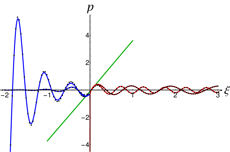
(a) $\rho=1.5^{4}$, $\varepsilon=0.1$

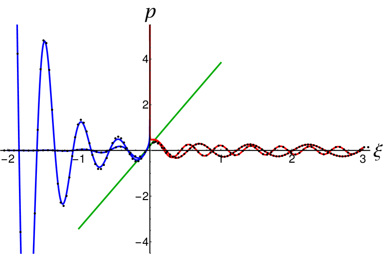
(b) $\rho=1.5^{4}$, $\varepsilon=0.12$

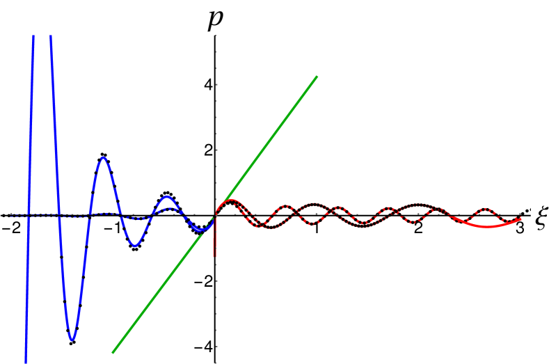
(c) $\rho=1.4^{4}$, $\varepsilon=0.1$

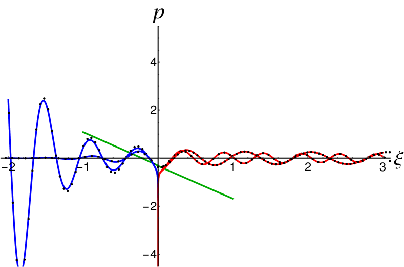
(d) $\rho=1.6^{4}$, $\varepsilon=0.1$

Figure 4: Solid lines represent the approximate solutions: red for $\Lambda>0$ in Eq. (36),(37), blue for $\Lambda<0$ in Eq. (38),(39), green for the approximation across the turning point in Eq. Eq. 43. Each dot is the numerically calculated contour integral, Eq. Eq. 25 along the SDC $C_{s}$ for a given $\xi$. Note that the approximation away from the turning point estimates the solution well, while it diverges at the turning point but where the final approximation captures the transition from an exponentially growing to an exponentially decreasing solution. These plots also serve as a verification of the final form of expression, Eq. 43, that is the chosen complex root of $(-1)^{6}$, in various situations.

Note that this knowledge of the solution behaviour reveals that the envelope is $\mathcal{O}\left(1\right)$ near the turning point, and the leading order behaviour is actually a rescaled Airy function as follows from Eq. 42 and Eq. 62,

(44) $$p\sim\underbrace{2\pi ie^{i\frac{1}{\varepsilon^{*}}\frac{8}{5}}(\varepsilon^{*})^{1/3}{M_{-}(0)}}_{\mbox{constant}}\mathrm{Ai}\left((-i)^{3/2}(\varepsilon^{*})^{2/3}\Lambda(\xi)\right),{\mbox{ as }\xi\to 0}.$$

Hence, the decay rates of the pattern tails correspond to the envelope behaviour of the Airy function matching those identified above in the outer WKB solution, as in Eqs. Eq. 36-Eq. 39.

4 Simulations of Heterogeneous Pattern Localisation

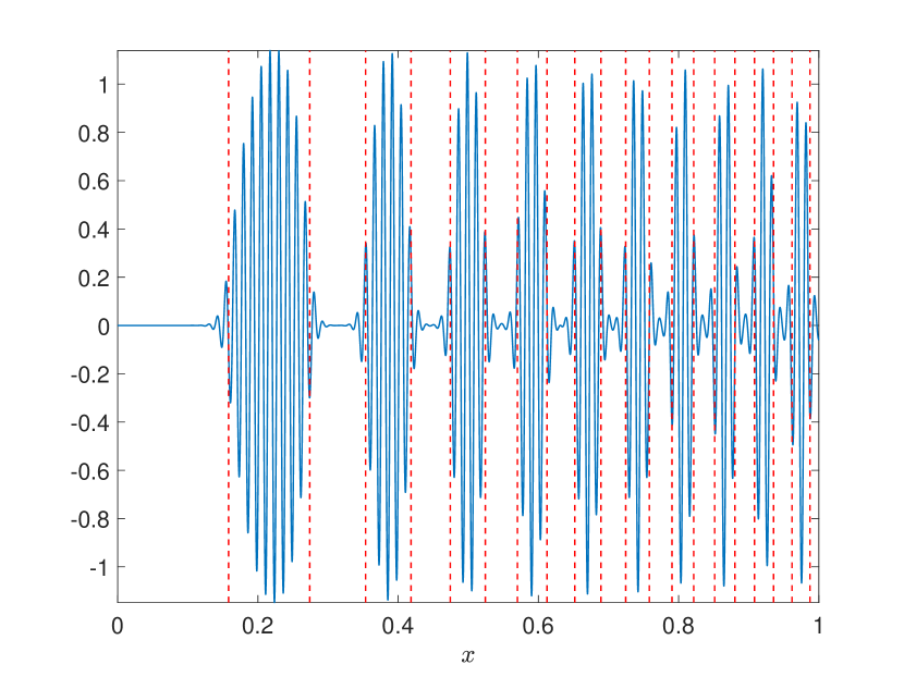
(a) $N(u)=-u^{3}$, $\varepsilon=0.002$

(b) $N(u)=-u^{3}$, $\varepsilon=0.0005$

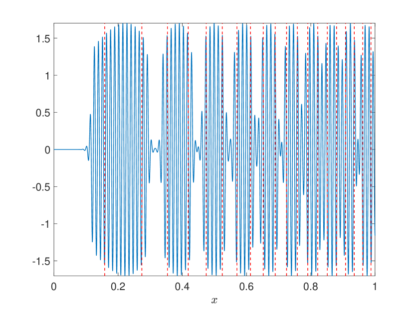
(c) $N(u)=2u^{3}-u^{5}$, $\varepsilon=0.002$

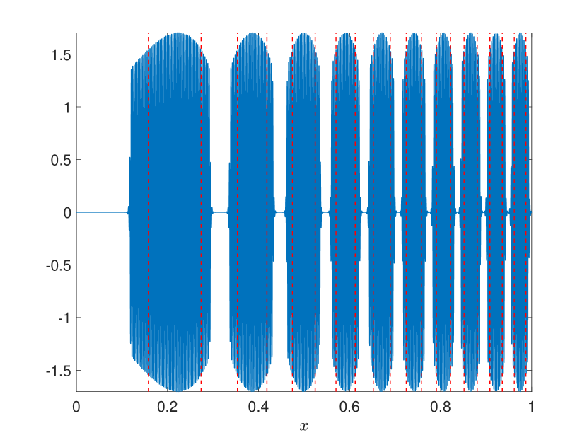
(d) $N(u)=2u^{3}-u^{5}$, $\varepsilon=0.0005$

Figure 5: Solutions $u(x)$ of Eq. 1 (blue solid curves) with $r(x)=-\cos(20\pi x^{2})$ and varying nonlinearity $N(u)$ and $\varepsilon$. Panels (a) and (b) are the cubic case corresponding to a locally supercritical nonlinearity, whereas (c) and (d) are a cubic-quintic nonlinearity corresponding to a locally subcritical instability. The dashed red vertical lines indicate where $r(x)=0$, and hence where a naive theory would predict patterning confinement. Simulation details can be found in Appendix B.

Here we show how a notion of ‘local criticality’ can impact the extent of patterning, and influence the tails of regions exhibiting confined patterns. We numerically simulated a large set of choices of the nonlinearity $N(u)$, focusing on polynomials up to seventh degree, a variety of trigonometric and more complex kinds of heterogeneity $r(x)$, as well as how the resulting solutions behave as $\varepsilon$ is varied. We refer to Appendix B for details of our numerical methods, as well as for details of an implementation of the model using a rapid interactive web simulator [51] that can be found at this simulation link. Below we present a small subset of these simulations to illustrate what we have learned, organized by the qualitative types of behaviour observed.

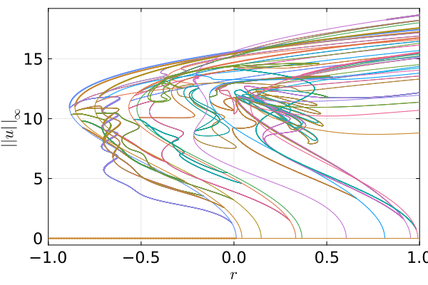
(a)

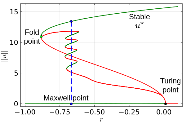
(b)

Figure 6: Bifurcation diagrams corresponding to steady state solutions of Eq. 4 as $r$ is varied for $N(u)=2u^{3}-u^{5}$ and $\varepsilon=0.01$. Panel (a) shows all connected primary, secondary, and ternary solution branches, whereas (b) focuses on the main branch emanating from the subcritical instability, leading to a stable branch after a secondary fold bifurcation. Stability in (a) is indicated by thicker curves being stable, whereas in (b) stability is indicated with green curves as stable and red dashed curves as unstable. We also indicate the approximate Maxwell point using a blue dashed vertical line, with localised solution branches ‘snaking’ around this point. Details about the continuation algorithm using BifurcationKit [50] can be found in Appendix B.

We first show in panels (a) and (b) of Fig. 5 that the linear theory developed predicts patterning regions even for complicated spatial heterogeneity $r(x)$ (in contrast to the simple heterogeneity of Fig. 1), as long as the nonlinearity leads to a locally supercritical bifurcation. As expected, for sufficiently small $\varepsilon$, the pattern formation is confined approximately to regions where $r(x)>0$, with tails that depend both on $\varepsilon$ and also on $|r^{\prime}(x)|$ locally, which increases with $x$ in these simulations. Note that this dependence is exactly encoded in Eq. 44, where $\varepsilon^{*}=\varepsilon\rho\approx\varepsilon r^{\prime}(x)$. In panels (c) and (d), we change the nonlinearity such that the corresponding spatially homogeneous model exhibits a subcritical instability for $r=0$. In this case, the confinement is no longer predicted well by the linear theory, even for small $\varepsilon$. We also observe that the tails confining the patterning regions appear more rapid than in the supercritical case, as one might expect from a larger amplitude solution rapidly losing stability at $x$ changes.

To understand this, we make use of the bifurcation structure of the homogeneous problem Eq. 4 in the vicinity of a subcritical Turing bifurcation. We numerically continue a solution, using the same nonlinearity $N(u)=2u^{3}-u^{5}$ as in Fig. 5(c)-(d), and plot the resulting branched structure in Fig. 6. Panel (a) shows that there are an enormous number of branches even in the homogeneous case, though we will be most interested in the main/topmost (green) stable branch depicted in panel (b), as this branch will correspond to domain-filling Turing patterns. Denoting this equilibrium patterned solution with $u^{*}$, we can compute its energy $E\left(u^{*}|_{r}\right)$ using Eq. 3 as a function of $r$ along the branch. Note that $E\left(u^{*}|_{r=0}\right)>0$ in all of the subcritical bifurcations we explored, and that the energy of this branch decreases as $r$ decreases. We define the Maxwell point of this domain-filling pattern branch (denoted as $\tilde{r}$) to be the point where the patterned solution and the trivial solution $u=0$ are equally energetically favorable (i.e. $E\left(u^{*}|_{r=\tilde{r}}\right)=E(0)$). This point is shown in Fig. 6(b) as the dashed blue line, as it tends to organize branches of localised solutions [3]. As we simulate solutions to the heterogeneous system Eq. 1, we locally compute the values of $r$ where a corresponding homogeneous problem undergoes the fold bifurcation of the patterned state (the solid green circle in Fig. 6(b)), as well as the corresponding Maxwell point.

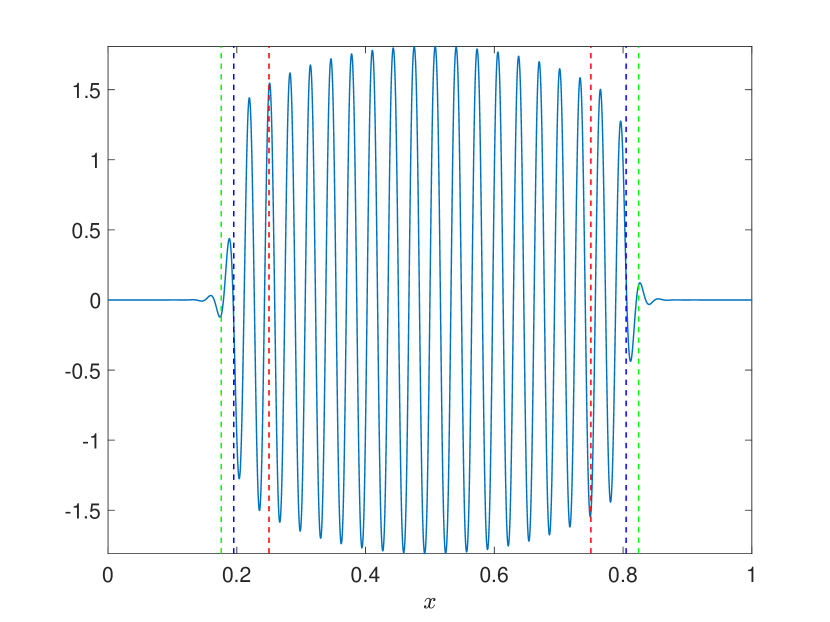
(a) $r(x)=-2\cos(2\pi x)$, $\varepsilon=0.005$

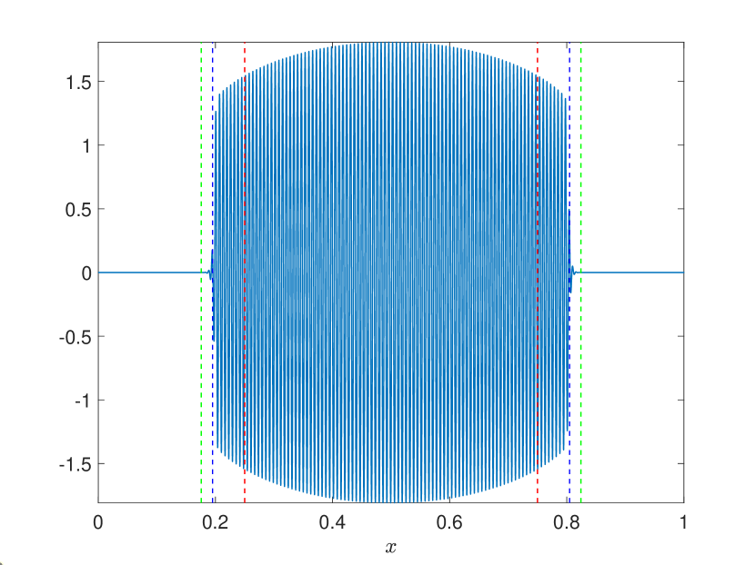
(b) $r(x)=-2\cos(2\pi x)$, $\varepsilon=0.001$

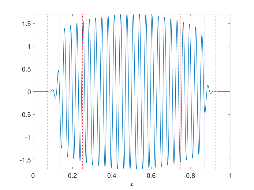
(c) $r(x)=-\cos(2\pi x)$, $\varepsilon=0.005$

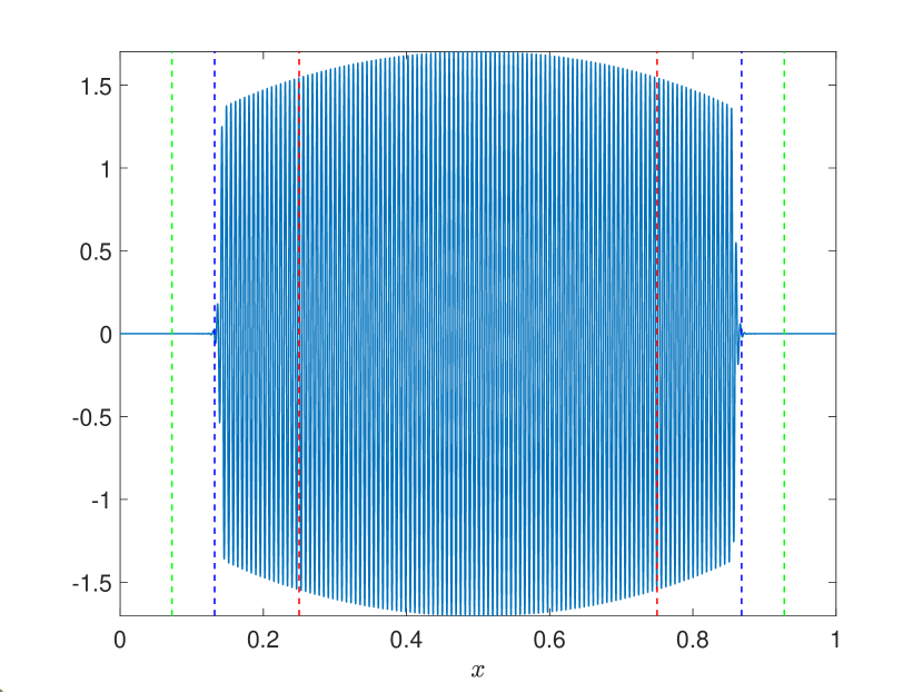
(d) $r(x)=-\cos(2\pi x)$, $\varepsilon=0.001$

(e) $r(x)=-0.7\cos(2\pi x)$, $\varepsilon=0.005$

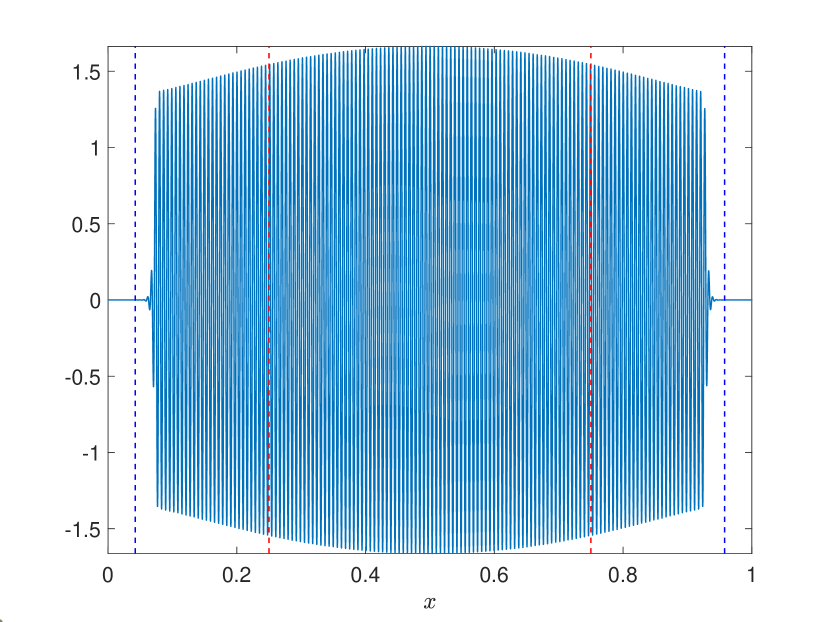
(f) $r(x)=-0.7\cos(2\pi x)$, $\varepsilon=0.001$

Figure 7: Solutions $u(x)$ of Eq. 1 (blue solid curves) with $N(u)=2u^{3}-u^{5}$ and varying heterogeneity $r(x)$ and $\varepsilon$. The dashed red vertical lines indicate where $r(x)=0$, the dashed blue lines correspond to where $E(u^{*})=0$, and the dashed green lines correspond to a local fold bifurcation as described in the text (which is now outside of the domain in panels (e) and (f)). Simulation details can be found in Appendix B.

We first consider varying the amplitude of a simple cosine heterogeneity in the cubic-quintic case. We plot solutions in Fig. 7, using vertical red lines to denote local Turing conditions, vertical blue lines to denote local Maxwell points, and vertical green lines to denote local fold points. As before, we observe a sharp drop in pattern amplitude, particularly for smaller values of $\varepsilon$ (cf Fig. 1). Roughly speaking, the Turing and fold points seem to fail to locate the region of confinement, whereas the Maxwell point approximates it well for most choices of $r(x)$ and $\varepsilon$. We do observe noticeable disagreement in panel (f), and for many other nonlinearities we see different kinds of disagreements with the local theory proposed here, but nevertheless find some evidence that local Maxwell points can predict pattern confinement, particularly for odd-ordered nonlinearities with moderate amplitude heterogeneities. As one might expect, in the subcritical case the local linear stability theory presented in Section 2 fails in all cases to account for the confinement of the pattern, though it is usually a subset of the patterning regions found in most cases (with some exceptions, as noted below).

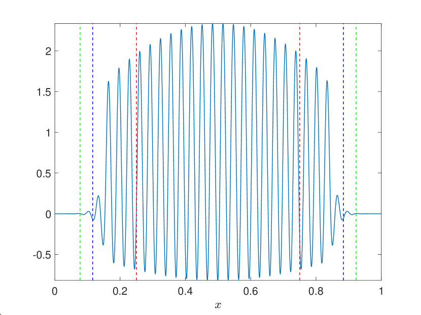
(a) $r(x)=-0.6\cos(2\pi x)$, $\varepsilon=0.005$

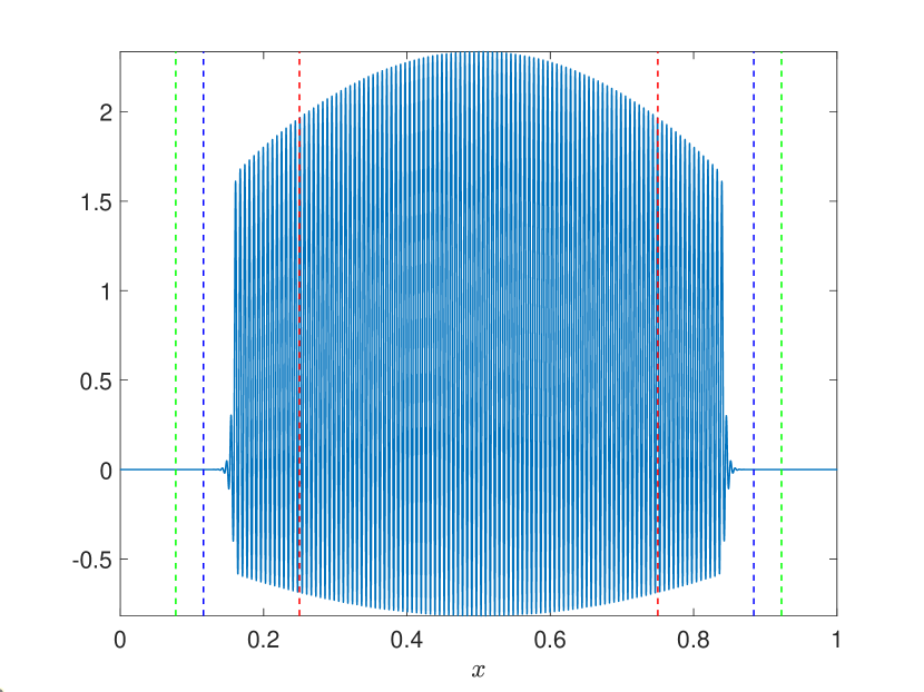
(b) $r(x)=-0.6\cos(2\pi x)$, $\varepsilon=0.0005$

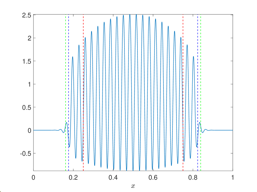
(c) $r(x)=-\cos(2\pi x)$, $\varepsilon=0.005$

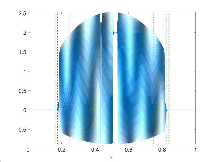
(d) $r(x)=-\cos(2\pi x)$, $\varepsilon=0.0005$

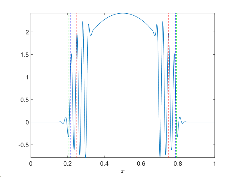
(e) $r(x)=-2\cos(2\pi x)$, $\varepsilon=0.005$

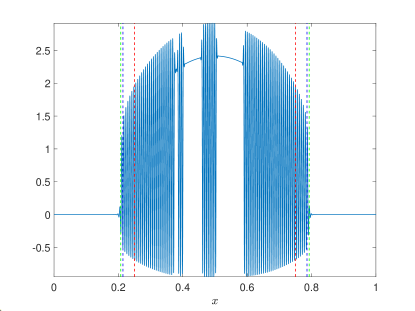
(f) $r(x)=-2\cos(2\pi x)$, $\varepsilon=0.0005$

Figure 8: Solutions $u(x)$ of Eq. 1 (blue solid curves) with $N(u)=2u^{2}-u^{3}$, varying $r(x)$ and $\varepsilon$. The dashed red vertical lines indicate where $r(x)=0$, the dashed blue lines correspond to where $E(u^{*})=0$, and the green lines correspond to a local fold bifurcation as described in the text. Simulation details can be found in Appendix B.

In contrast, nonlinearities including even-ordered terms typically led to solutions where the local Maxwell point only occasionally predicted the confined pattern region. Some examples are shown in Fig. 8. Perhaps more strikingly, this nonlinearity also led to local regions of the solution approximately following a different local equilibrium (that is, one of the polynomial solutions of Eq. 1 one obtains setting $\varepsilon=0$). Different simulations with varied initial conditions (e.g. using the same random perturbations of $u=0$ but taking a different random seed) also led to solutions where different parts of the domain contained oscillatory ‘patterned’ states interspersed with more smoothly varying ‘local’ equilibria. While it appears the Maxwell point idea works better for larger amplitudes, this is observed to be extensively driven by larger amplitudes drastically increasing the speed at which the solution moves through the bifurcation. Hence, a more accurate theory of the slow passage through this structure must account not only for the value of $r(x)$ where the pattern is no longer energetically favorable, but also the nonlinearity and the speed at which the heterogeneous solution passes this point.

The existence of other local equilibria does not only plague the locally subcritical case. In Fig. 9, we use locally supercritical nonlinearities but a much larger heterogeneity to observe that these intermittent solutions can also create distorted patterns in these cases. While the patterned states are indeed approximately confined by the local Turing instability criterion predicted in Section 2 (that is, $r(x)\approx 0)$), the patterned state can be made up of a variety of intermittent states involving these branches of local equilibria. Which solution emerges then is seemingly sensitively dependent on the initial condition, and we are unaware of any simple theory capable of explaining why some kinds of structures are observed more often than others, noting that any notion of basins of attraction for such solutions will likely be complex. We note that the simulations shown in Fig. 9, as well as the final two panels of Fig. 8, violate the condition Eq. 6, though in the patterned region this condition is not so important as the solution is already far from the trivial equilibrium where linear stability is valid.

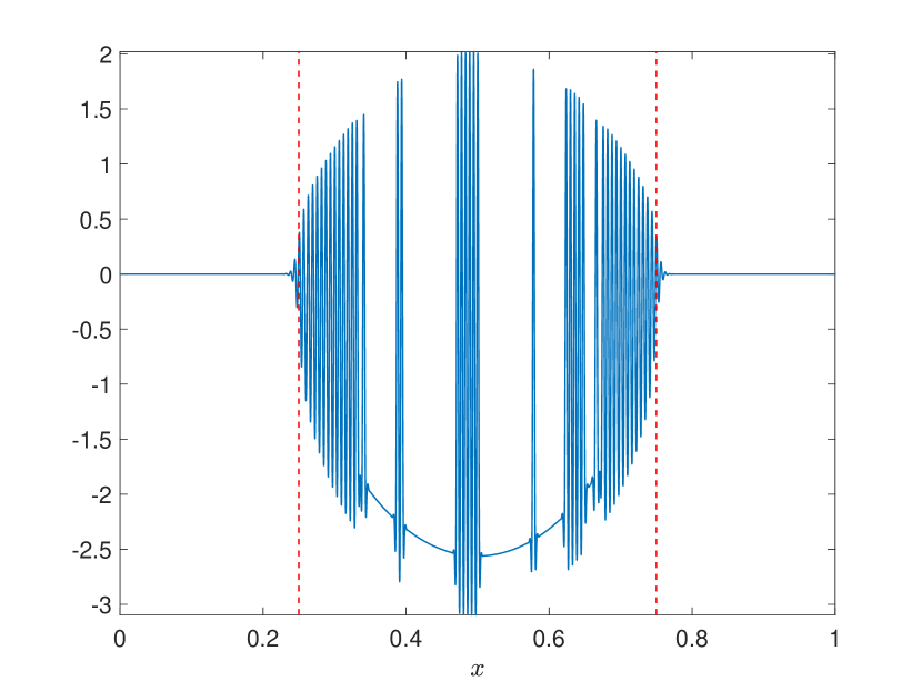
(a) $N(u)=-u^{2}-u^{3}$

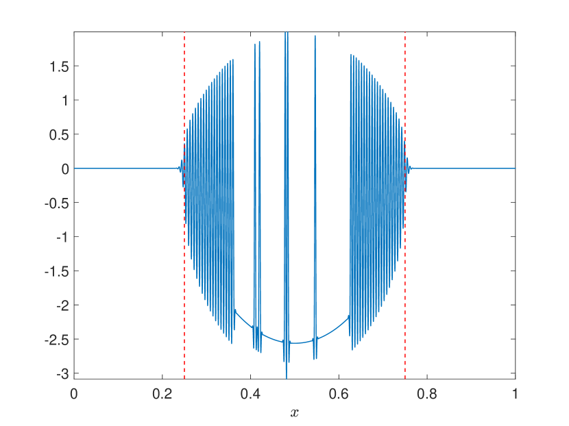
(b) $N(u)=-u^{2}-u^{3}$

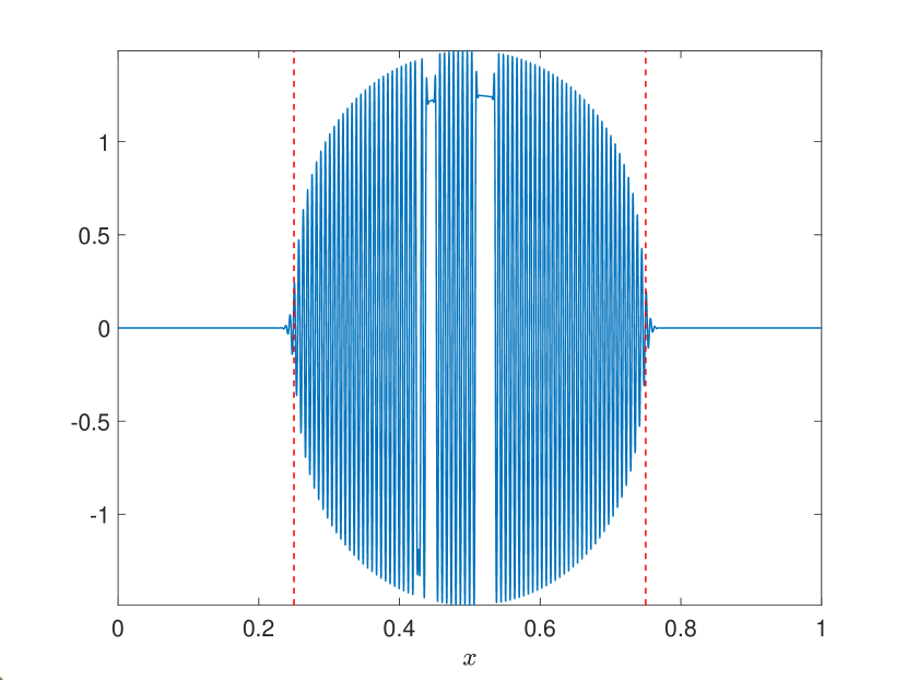
(c) $N(u)=-u^{3}-u^{5}$

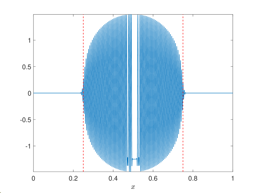
(d) $N(u)=-u^{3}-u^{5}$

Figure 9: Solutions $u(x)$ of Eq. 1 (blue solid curves) with $r(x)=-5\cos(2\pi x)$, $\varepsilon=0.001$, varying $N(u)$ and the random initial conditions. The dashed red vertical lines indicate where $r(x)=0$. Simulation details can be found in Appendix B.

We end this section by noting that we only exhibited a handful of the solutions produced in order to focus on the essence of the behaviours we observed. We also explored a more general heterogeneous model of the form,

(45) $$\frac{\partial u}{\partial t}=r(x)u-\left(q(x)^{2}+\varepsilon^{2}\frac{\partial^{2}}{\partial x^{2}}\right)^{2}u+N(u,x),\quad\quad\quad x\in[0,1],$$

though chose to focus our attention on the simpler model given by $q(x)=1$ and $N(u,x)=N(u)$ to present key exemplars of what we found more generally. As long as $\varepsilon$ was sufficiently small (e.g. we always took $\varepsilon\leq 0.01$), locally supercritical nonlinearities always gave rise to confined regions of patterning, with tails near the boundary behaving as predicted by Eq. 44. In contrast, locally subcritical instabilities had larger regions of patterning which fell rapidly back to the trivial state $u=0$. These regions of pattern confinement in the subcritical cases could sometimes be predicted by looking for a local Maxwell point, but in other cases could not. In all cases, sufficiently large amplitude heterogeneity leading to many local equilibria could give rise to disconnected regions of pattern formation, somewhat independent of the nature of the heterogeneity and nonlinearity involved, and the final form of the observed pattern became more sensitive to initial data.

5 Discussion

We started this paper by asking: given an observed spatial pattern, what can we say about the underlying mechanism that generated this localisation? To begin formulating an answer, we studied a simple model of slow heterogeneity in the Swift-Hohenberg equation. We extended ideas from the reaction-(cross)-diffusion literature [33, 19] to provide an asymptotic justification of a local Turing instability theory, and a resolution to the boundary-layer behaviour of this asymptotic theory. We then explored a variety of different kinds of heterogeneity and nonlinearity, finding that this theory does well for predicting confinement of patterns in the case of locally supercritical nonlinearities, but fails to predict regions of pattern confinement in locally subcritical cases. Despite the simplicity of the 1D model chosen, there seem to be large gaps in our understanding of heterogeneous systems in the presence of subcritical instabilities.

There are numerous direct extensions of what we have studied here. While we have provided numerical and theoretical evidence that locally supercritical instabilities lead to gradually-decaying tails of patterning in the specific cases explored, more generality remains to be shown, as does any analytical support that subcritical instabilities should always coincide with a more sudden decay in amplitude. The latter is what one may expect from the heteroclinic connection between different equilibria using ideas from spatial dynamics, (e.g. one can imagine falling off the top branch in Fig. 6(b) onto the trivial state via such a connection). The precise unfolding of such a heteroclinic connection is likely to involve effects that are beyond all orders in $\varepsilon$. Such exponential asymptotics approaches to localised pattern formation have been carried out in the spatially homogeneous setting (see [14, 18] and references therein), but have not, to our knowledge, been applied to spatially heterogeneous systems. More generally, the interaction between snaking-induced localisation and heterogeneity-induced localisation is especially relevant to understand from an applied point of view. We have provided evidence that slow Airy-like envelopes may correspond to supercritical heterogeneity-induced bifurcations for the cases considered, but we cannot distinguish between more rapid decay due to heterogeneity or snaking in the subcritical case in general.

Besides these ideas, one can imagine studying these phenomena in other models, in higher dimensions (such as in the work on multidimensional localised snaking solutions [20, 7]), or pursuing much more rigorous approaches than our simple formal asymptotics and numerical explorations (as in [29, 23]). Recent work has extended these ideas to spatiotemporal forcing of pattern-forming systems, determining parameter regimes where the system does or does not follow a naive quasi-static prediction of when and where pattern formation occurs, depending on the magnitude and frequency of the forcing [17]. We remark that this extension crucially required the assumption of a locally supercritical bifurcation, as the subcritical case is, as demonstrated here, vastly more intricate. Entirely alternative approaches, such as directly looking at how heterogeneity itself induces bifurcations [49], or considering the impact of introducing heterogeneity on localised solutions coming from homoclinic snaking mechanisms [25], may also prove useful.

Despite the complexity observed in our simulations, the existence of the energy functional Eq. 3 precludes the possibility of long-time spatiotemporal states, heterogeneity-induced [32, 27] or those arising from local Hopf instabilities [41]. The existence of multiple spatially homogeneous equilibria can likely induce a range of nontrivial behaviours such as Turing instabilities which fail to form patterned states [30], or complex dynamics only sometimes understood via local analogues such as heteroclinic connections between homogeneous solutions [41]. Versions of the Swift-Hohenberg equation with broken nonlinear symmetries [22], or with non-variational structure [10], have been shown to exhibit a variety of interesting behaviours, and would be obvious models to consider to generalize the ideas presented here.

Fig. 6(a), despite only showing a subset of solution branches, demonstrates a variety of branches apparent in the homogeneous form of our model as a single parameter is varied. We anticipate that such pictures will only become more complicated with spatial heterogeneity. Preliminary bifurcation analyses (not shown) indicate that ‘adding’ a heterogeneous forcing to systems and following the branches from such diagrams can effectively shatter these continuous branches, leading to many disconnected branches. While local bifurcation-theoretic approaches (such as those used in this paper and essentially all of the existing literature) are important for understanding some aspects of these systems, we also want to highlight that there is a growing need to understand more global dynamics of models with heterogeneity and multiple equilibria.

Appendix A Details of inner solution asymptotics

A.1 Regions of validity of the outer solution

The inner problem for $x=a$ such that $r(a)=\lambda$ is

$$0=\varepsilon^{4}p^{(4)}+2\varepsilon^{2}p^{\prime\prime}+p-{\rho(x-a)}p,$$

where $\rho={r^{\prime}(a)}$. We use the more general WKB ansatz,

$$p\sim{\exp}\left({\sum_{n=0}}\frac{1}{\varepsilon}\varepsilon^{n}S_{n}\right).$$

By a dominant balance argument, we get

(46) $$S_{0}\sim i{(x-a)},\quad S_{1}\sim-\frac{1}{4}\ln{(x-a)},\quad S_{2}\sim\frac{{(x-a)}^{-3/2}}{\sqrt{|\rho}|}.$$

As the WKB approximation is valid for ${|S_{0}|}/\varepsilon\gg{|S_{1}|}\gg\varepsilon{|S_{2}|}$, we get the region of validity as

$${|x-a|}\gg\varepsilon^{2/3}\rho^{-1/3}.$$

Similarly, considering another turning point where $1=\sqrt{r(a)-\lambda}$, the region of validity of the local WKB approximation is

$${|x-a|}\gg\varepsilon^{2/3}\rho^{-1/3}.$$

Therefore, when $\varepsilon$ is sufficiently small and the $u=0$ solution is stable, we can use the WKB solution and be sufficiently far away from this second possible turning point.

A.2 Asymptotics of the integral solution for $\Lambda>0$

To further illustrate the asymptotics from the main text, we add plots of the SDC, tangent at the saddle and asymptotes for the second saddle $s_{+-}$ together with contour plot of $\imaginary(\psi)$ in Fig. 10 and Fig. 11.

(a) SDC in the complex plane.

(b) Real part of $\psi$ along the contour ($x$ axis being the parameter $t=a$ along the contour) confirming that it is the (steepest) descent curve.

Figure 10: Steepest descent contour for $\Lambda=0.6$ passing through $s_{+-}$, with $s_{+-}=0.5$, $\alpha_{+-}=-0.2$ and the tangent angle of the SDC at $s_{+-}$ given by $3\pi/4$. The asymptotes in panel (a) are at the angles $\pi/2$ and $17\pi/10$, with one dashed line indicating the latter asymptote and a second dashed line depicting the tangent at the saddle, while the asymptote of angle $\pi/2$ coincides with the axis.

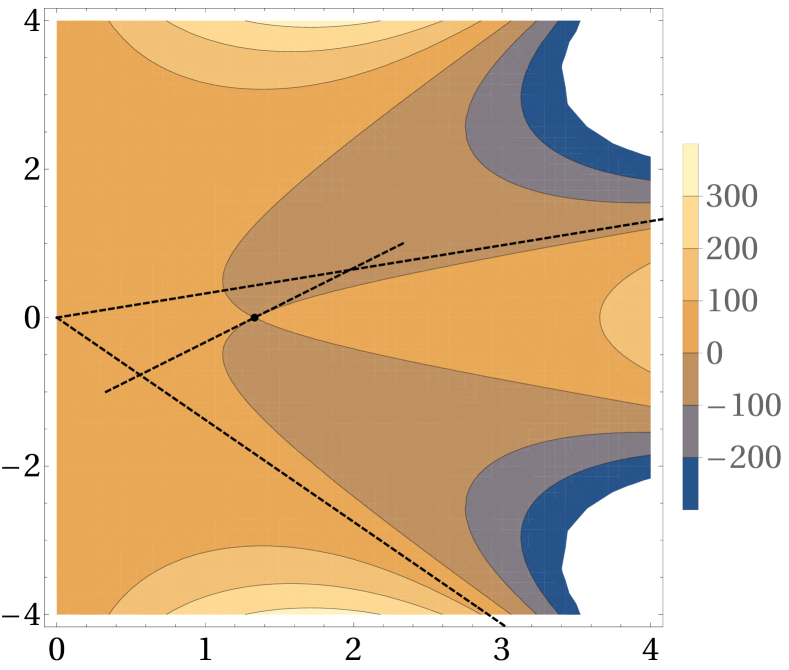
(a) Contour lines of the imaginary part of $\psi$ in the complex plane.

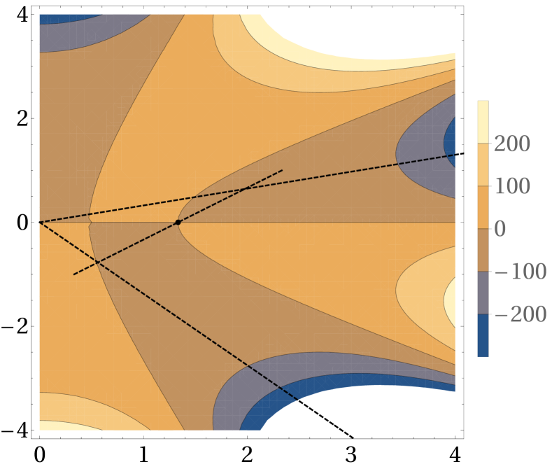
(b) Contour lines of the real part of $\psi$ in the complex plane.

Figure 11: The landscape of real and imaginary part of $\psi$ together with the highlighted location of the SDC passing through the saddle $s_{++}$ together with the calculated asymptotes and tangent at the saddle. Here, $\Lambda=0.6$.

A.3 Asymptotics of the integral solution for $\Lambda<0$

In the situation when $\Lambda<0$, saddles are not located on the real line and their locations are given by

(47) $$s_{++} :=+(1-\Lambda)^{1/4}(\cos(\varphi)+i\sin(\varphi)),$$

(48) $$s_{+-} :=-(1-\Lambda)^{1/4}(\cos(\varphi)-i\sin(\varphi))=\bar{s}_{++},$$

$$s_{-+} =-s_{+-},s_{--}=-s_{++},$$

where $\varphi=\frac{1}{2}\arctan(\sqrt{-\Lambda})$ and again we drop $s_{-+}$ and $s_{--}$ due to the symmetry.

The SDC can be parametrised in the same way as in the positive case, hence the asymptotes are the same. However, the directions of the steepest descent at the saddles $s_{++}$, $s_{+-}$ depend on $\Lambda$ (and are not constants as in the case $\Lambda>0$). They are given by angles

$$\phi_{++} =\mathrm{Arg}\left[\left((-i+\sqrt{-\Lambda})\left[(-1+\sqrt{1-\Lambda})\cos(\varphi)+i(1+\sqrt{1-\Lambda})\right]\right)^{-1/2}\right],$$

$$\phi_{+-} =\mathrm{Arg}\left[\left((-i-\sqrt{-\Lambda})\left[(-1+\sqrt{1-\Lambda})\cos(\varphi)-i(1+\sqrt{1-\Lambda})\right]\right)^{-1/2}\right],$$

where the subscript denotes the corresponding saddle. In Fig. 12 we illustrate the dependence by plotting these angles for (complex arguments of) all the four saddles. Note that one can expand this expression for the tangent angle for small negative $\Lambda$ and get that the tangent angle of the SDC at $s_{++}$ approaches $0$ while taking the value $-\pi/2$ at $s_{+-}$. Hence there is a discontinuity of the contour across the turning point $\Lambda=0$. This is not unexpected, as two pairs of saddles coalesce into one and then split.

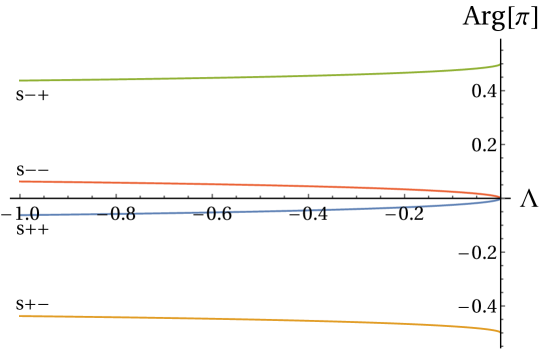
Figure 12: The numerically evaluated tangent angles of the SDC at the saddles as a function of $\Lambda<0$ following from the expression for $\phi_{++}$ and the other three angles in the main text. The $y$-axis is in multiples of $\pi$.

One can show that the two complex conjugate saddles, $s_{++}$ and $s_{+-}$, have the same value of $\imaginary(\psi)$ and hence lie on the same SDC. In addition, $\real(\psi)$ is larger at $s_{+-}$, hence the steepest descent contour of $s_{+-}$ passes through $s_{++}$ on descent. We illustrate the SDC with a particular choice $\Lambda=-0.7$ in Figures 13, 14, and 15.

(a) SDC in the complex plane for $s_{++}$.

(b) Real part of $\psi$ along the contour ($x$ axis being the parameter $t=a$ along the contour) confirming that it is the (steepest) descent curve.

Figure 13: Steepest descent contour for $\Lambda=-0.7$ passing through $s_{++}$. The dashed lines indicate the revealed asymptote at one end (being $\pi/10$), the other being $\pi/2$.

(a) SDC in the complex plane.

(b) Real part of $\psi$ along the contour ($x$ axis being the parameter $t=a$ along the contour) confirming that it is the (steepest) descent curve.

Figure 14: Steepest descent contour for $\Lambda=-0.7$ passing through $s_{+-}$ (the highlighted point) but also through $s_{++}$ being the complex conjugate of $s_{+-}$. The dashed lines indicate the revealed asymptotes (the new one being $17\pi/10$). Note that the real part of $\psi$ is greater at $s_{+-}$ than at $s_{++}$ and, as a result, the SDC corresponding to $s_{+-}$ continues along the SDC of $s_{++}$ once the second saddle is reached (arbitrarily choosing one of the two halves).

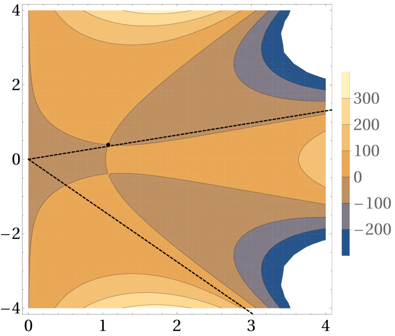
(a) Contour lines of the imaginary part of $\psi$ in the complex plane.

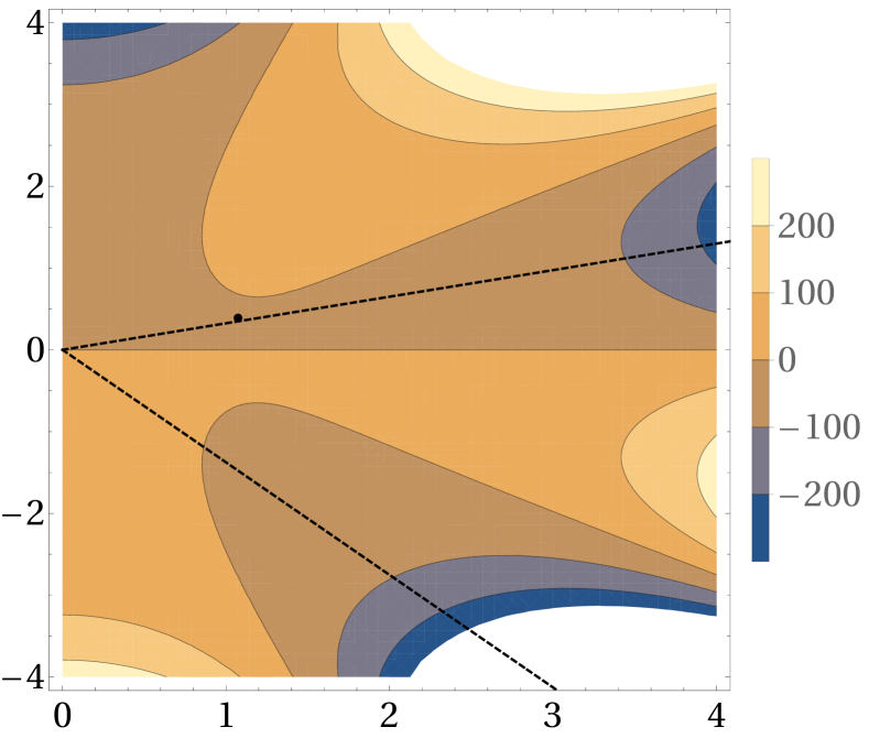
(b) Contour lines of the real part of $\psi$ in the complex plane.

Figure 15: The landscape of real and imaginary part of $\psi$ together with the highlighted location of the SDC passing through the saddle $s_{++}$ together with the calculated asymptotes and tangent at the saddle. Here, $\Lambda=-0.7$.

The approach to the contour integral approximation is the same as in the positive case. We again have four independent solutions corresponding to saddles $s_{++},~{}s_{+-}$ and note that due to $\real(\psi)|_{s_{+-}}>\real(\psi)|_{s_{++}}$ the contribution of the neighbourhood of $s_{++}$ to the contour integral along the $s_{+-}$ contour (passing through $s_{++}$) is subleading.

We first evaluate $\psi$ and its second derivative at the saddle $s_{++}$. We have

$$\psi_{++} =-\left[184+56G-132\Lambda+120\frac{\Lambda}{G}\frac{1}{\sin^{2}(\varphi)}+15\frac{\Lambda^{2}}{G^{2}}\frac{1}{\sin^{4}\varphi}\right]$$

$$\qquad\times\frac{(1-\Lambda)^{1/4}\sin(\varphi)}{240}+i\left[\frac{4}{15}\left(1+G-3\Lambda\right)G^{1/2}\cos(\varphi)\right],$$

$$\psi_{++}^{\prime\prime} =4(1-\Lambda)^{-1/4}(i-\sqrt{-\Lambda})\left[\left(-1+G\right)\cos(\varphi)+i\left(1+G\right)\sin(\varphi)\right]$$

$$=4G^{-1/2}\bigg{[}\sqrt{-\Lambda}\left(-1+G\right)\cos(\varphi)+\left(1+G\right)\sin(\varphi)$$

$$\qquad+i\left(\left(1-(1-\Lambda)^{1/2}\right)\cos(\varphi)+\sqrt{-\Lambda}\left(1+(1-\Lambda)^{1/2}\right)\sin(\varphi)\right)\bigg{]},$$

where $G=(1-\Lambda)^{1/2}$ to slightly simplify the typesetting. Hence, the corresponding solution is approximately

(49) $$p_{++}(y)\sim\sqrt{2\varepsilon^{*}\pi}\cos\left(\frac{1}{\varepsilon^{*}}\frac{4}{15}\left(1+(1-\Lambda)^{1/2}-3\Lambda\right)(1-\Lambda)^{1/4}\cos(\varphi)\right)$$

$$\times\left(-\psi_{++}^{\prime\prime}e^{2i\theta_{++}}\right)^{-1/2}\exp\left[\left(-\frac{1}{\varepsilon^{*}}\frac{1}{240}(1-\Lambda)^{1/4}\sin(\varphi)\right)K\right],$$

where

(50) $$K=\left[184+56(1-\Lambda)^{1/2}-132\Lambda+120\frac{\Lambda}{(1-\Lambda)^{1/2}}\frac{1}{\sin^{2}(\varphi)}+15\frac{\Lambda^{2}}{1-\Lambda}\frac{1}{\sin^{4}\varphi}\right]$$

and $\phi_{++}$ is the angle of the SDC at $s_{++}$, see above. Note that there is another solution with $\sin$ instead of $\cos$ and $-\psi_{++}^{\prime\prime}e^{2i\phi_{++}}>0$ by the construction of the steepest descent curve.

Now, let us focus on the other saddle, $s_{+-}$. One can show that

$$\psi_{+-}=-\psi_{++},\quad\phi_{+-}=\frac{\pi}{2}-\phi_{++},\quad-\psi_{+-}^{\prime\prime}=-\overline{\psi_{++}^{\prime\prime}},$$

and hence

$$p_{+-}(y) \sim\sqrt{2\varepsilon^{*}\pi}\cos\left(\frac{1}{\varepsilon^{*}}\frac{4}{15}\left(1+(1-\Lambda)^{1/2}-3\Lambda\right)(1-\Lambda)^{1/4}\cos(\varphi)\right)$$

(51) $$\times\left(-\psi_{+-}^{\prime\prime}e^{2i\theta_{+-}}\right)^{-1/2}\exp\left[\left(\frac{1}{\varepsilon^{*}}\frac{1}{240}(1-\Lambda)^{1/4}\sin(\varphi)\right)K\right],$$

with $K$ similarly defined in Eq. 50. There is, again, an additional solution when replacing $\cos$ with $\sin$.

A.4 Approximation of the contour integral near the turning point

As stated in the main text, sufficiently close to the turning point, the approximations invoking Laplace’s method no longer work. We shall take the advantage of the fact that each of the two pairs of the real saddles coalesce as $\Lambda\to 0^{+}$ and then separate out into two complex conjugate pairs once $\Lambda$ has become negative, so that for $0<|\Lambda|\ll 1$ the saddles are close to coalescence.

We thus proceed here according to [45, Chapter 23], [36, Chapter 9], [15] where the main idea is to find and use a suitable change of variables so that one can use the known integral representation and asymptotics of Airy functions. Namely, it holds that

(52) $$\frac{1}{2\pi i}\int_{C_{\mathrm{Ai}}}e^{\frac{1}{\varepsilon}(\frac{1}{3}t^{3}-\eta t)}f(t)\differential t\sim\varepsilon^{1/3}\left({M(\eta)}+\mathcal{O}\left(\varepsilon\right)\right)\mathrm{Ai}\left(\eta\varepsilon^{-2/3}\right)\\ -\varepsilon^{2/3}\left({N(\eta)}+\mathcal{O}\left(\varepsilon\right)\right)\mathrm{Ai}^{\prime}\left(\eta\varepsilon^{-2/3}\right),$$

as $\varepsilon\to 0^{+}$ with $M(\eta)=\frac{1}{2}\left(f(\sqrt{\eta})+f(-\sqrt{\eta})\right)$, $N(\eta)=\frac{1}{2}\frac{1}{\sqrt{\eta}}\left(f(\sqrt{\eta})-f(-\sqrt{\eta})\right)$ and where the contour $C_{\mathrm{Ai}}$ is one of the three Airy contours with the asymptotes of $(-1)^{1/3}$.

To this end, a cubic transformation is used such that the two coalescing saddles are mapped onto the two extrema of the cubic. In particular, we consider

(53) $$\Xi(t)=\frac{1}{3}t^{3}-\eta t+A,$$

and we look for the values of parameters $A,~{}\eta$ such that the two saddles of the cubic, that is $t_{\pm}=\pm\sqrt{\eta}$, match the two coalescing saddles $s_{+-},~{}s_{++}$, and below we have the latter matches $t_{-}$. Hence, we look for a transformation $s\to t$ such that

(54) $$\psi(s)=\Xi(t)\mbox{ at the two saddles.}$$

That is

(55) $$i\left[(1-\Lambda)(1\pm\Lambda^{1/2})^{1/2}-\frac{2}{3}(1\pm\Lambda^{1/2})^{3/2}+\frac{1}{5}(1\pm\Lambda^{1/2})^{5/2}\right]=\mp\frac{2}{3}\eta^{3/2}+A.$$

Hence $2A=\psi(s_{++})+\psi(s_{+-})$, resulting in

(56) $$A =-\frac{2}{15}i\left[-2(s_{+-}+s_{++})+\sqrt{\Lambda}(s_{++}-s_{+-})+3\Lambda(s_{++}+s_{+-})\right]$$

$$\sim i\left(\frac{8}{15}-\Lambda\right)\mbox{ as }{\Lambda\to 0}.$$

Further, due to the sign choices, the saddle $s_{++}$ maps onto $t_{-}$, and hence

(57) $$\frac{2}{3}\eta^{3/2}=\frac{\psi(s_{++})-\psi(s_{+-})}{2},$$

and

(58) $$\eta^{3/2} =\frac{1}{5}i\left[2(s_{++}-s_{+-})-\sqrt{\Lambda}(s_{++}+s_{+-})+3\Lambda(s_{+-}-s_{++})\right]$$

$$\sim-i{\frac{1}{2}}\Lambda^{3/2}\mbox{ as }{\Lambda\to 0}.$$

This completes the specification of the cubic transformation $\Xi(t)$.

As our contour integral representation of the solution is of the form $\int_{C}\exp\left(\frac{1}{\varepsilon^{*}}\psi\right)$, the function $f$ in (40) follows from the transformation $s\to t$ as

(59) $$f(t)=\frac{\differential s}{\differential t}.$$

As the dominant contribution comes from the saddles, we expand both $\Xi$ and $\psi$ around $s_{++}$ as

$$\Xi(t) =\psi(s)$$

$$=\psi(s_{++})+\psi^{\prime\prime}(s_{++})\frac{1}{2}(s-s_{++})^{2}+\psi^{\prime\prime\prime}(s_{++})\frac{1}{6}(s-s_{++})^{3}+\mathcal{O}\left(s-s_{++}\right)^{4}$$

$$=\Xi(t_{-})+{\Xi^{\prime\prime}(t_{-})}\frac{1}{2}(t-t_{-})^{2}+\Xi^{\prime\prime\prime}(t_{-})\frac{1}{6}(t-t_{-})^{3}+\mathcal{O}\left(t-{t_{-}}\right)^{4},$$

and hence we identify $s(t)$ near $t=t_{-}$ as

$$s(t) ={s_{++}\pm\left(\frac{\Xi^{\prime\prime}}{\psi^{\prime\prime}}\right)^{1/2}(t-t_{-})\pm\frac{\Xi^{\prime\prime\prime}\mp\psi^{\prime\prime\prime}\left(\frac{\Xi^{\prime\prime}}{\psi^{\prime\prime}}\right)^{3/2}}{6(\Xi^{\prime\prime}\psi^{\prime\prime})^{1/2}}(t-t_{-})^{2}+\mathcal{O}\left(t-t_{-}\right)^{3}},$$

where we used $s(t_{-})=s_{++}$. Hence, we may now identify the sought function $f=$d$s/$d$t$ to sufficient accuracy for our requirements, as

$${f(t)=\pm\left(\frac{\Xi^{\prime\prime}}{\psi^{\prime\prime}}\right)^{1/2}\pm\frac{\Xi^{\prime\prime\prime}\mp\psi^{\prime\prime\prime}\left(\frac{\Xi^{\prime\prime}}{\psi^{\prime\prime}}\right)^{3/2}}{3(\Xi^{\prime\prime}\psi^{\prime\prime})^{1/2}}(t-t_{-})},$$

and the coefficients of the approximation (52) as

$${M_{\pm}}=\pm\left[\left(\frac{\Xi^{\prime\prime}}{\psi^{\prime\prime}}\right)^{1/2}+\sqrt{\eta}\frac{\Xi^{\prime\prime\prime}\mp\psi^{\prime\prime\prime}\left(\frac{\Xi^{\prime\prime}}{\psi^{\prime\prime}}\right)^{3/2}}{3(\Xi^{\prime\prime}\psi^{\prime\prime})^{1/2}}\right],\quad{N_{\pm}}=\left[\frac{\Xi^{\prime\prime\prime}\mp\psi^{\prime\prime\prime}\left(\frac{\Xi^{\prime\prime}}{\psi^{\prime\prime}}\right)^{3/2}}{3(\Xi^{\prime\prime}\psi^{\prime\prime})^{1/2}}\right],$$

where all derivatives of $\Xi$ are evaluated at $t_{-}$, while $\psi$ is evaluated at $s_{++}$.

Finally, note that the asymptotes of the SDC passing through $s_{++}$ have tangent angles of $\pi/10$ and $17\pi/10$ while $\psi(s)\sim i\frac{1}{5}s^{5}$ for large $s$. As $\Xi(t)\sim\frac{1}{3}t^{3}$ for large $t$, we can see that the cubic transformation transforms the integration contour into a contour with asymptotes being $\left(e^{i\pi/2}(e^{i\pi/10})^{5}\right)^{1/3}$ and $\left(e^{i\pi/2}(e^{i17\pi/10})^{5}\right)^{1/3}$, that is $(-1)^{1/3}$. Therefore we have that

(60) $$\int_{C}e^{\frac{1}{\varepsilon^{*}}\psi(s)}\differential s\sim\int_{\tilde{C}}e^{\frac{1}{\varepsilon^{*}}\Xi(t)}\frac{\differential s}{\differential t}\differential t,$$

with $\tilde{C}$ being one of the Airy contours.

As the largest contributions to the contour integral arise from the neighbourhood of the coalescing saddles, where $f(t)=\frac{\differential s}{\differential t}$ has been identified, we have

(61) $$\int_{C}e^{\frac{1}{\varepsilon^{*}}\psi(s)}\differential s\sim 2\pi ie^{\frac{A}{\varepsilon^{*}}}\left[(\varepsilon^{*})^{1/3}\mathrm{Ai}\left(L\right)(M_{\pm}+\mathcal{O}\left(\varepsilon^{*}\right))-(\varepsilon^{*})^{2/3}\mathrm{Ai}^{\prime}\left(L\right)(N_{\pm}+\mathcal{O}\left(\varepsilon^{*}\right))\right],$$

with $L=\eta(\varepsilon^{*})^{-2/3}$ for ease of presentation.

The final check consists in verifying the assumed analyticity of the solution in $\eta$ (and thus in $\Lambda$, i.e. in the spatial coordinate $y$). With the knowledge of $\eta(\Lambda)$, we may Taylor expand to reveal that

(62) $$M_{\pm}=\mathcal{O}\left(1\right)\mbox{ as }\Lambda\to 0,$$

but

(63) $$N_{+}=\mathcal{O}\left(\Lambda^{-1/2}\right),\quad N_{-}=\mathcal{O}\left(1\right)\mbox{ as }\Lambda\to 0.$$

Therefore, we conclude that the contour integral representation of the solution near the turning point is the real or imaginary part of

(64) $$p(\xi)\sim 2\pi ie^{\frac{1}{\varepsilon^{*}}A}\left[(\varepsilon^{*})^{1/3}\mathrm{Ai}\left(\eta/(\varepsilon^{*})^{2/3}\right)M_{-}-(\varepsilon^{*})^{2/3}\mathrm{Ai}^{\prime}\left(\eta/(\varepsilon^{*})^{2/3}\right)N_{-}\right],$$

with $A,\eta,M_{-},N_{-}$ given above and being functions of $\Lambda(\xi)$.

To explicitly see the behaviour across the turning point, we Taylor expand and obtain a continuous function

(65) $$p\sim\frac{\pi(\varepsilon^{*})^{1/3}}{6^{2/3}\Gamma(2/3)}(-1)^{1/6}\left(2i+(-1)^{2/3}\sqrt{\Lambda}+\frac{2}{\varepsilon^{*}}\Lambda\right)e^{\frac{1}{\varepsilon^{*}}\frac{8}{15}i}{\left(1+o(1)\right)},$$

where the $N_{-}$ contribution only generates terms within the $o(1)$ correction and we have $\varepsilon^{*}$ is small but fixed, while $\Lambda$ attains arbitrarily small values near the turning point, with $\Lambda/\varepsilon^{*}=y$. Recalling that the sought solution is the real or imaginary part of the contour integral and the presence of $(-1)^{1/6}$ leads to six branches of potential solutions, we have 12 potential approximations at the turning points, see Fig. 17.

To identify the correct approximation from all these potential solutions, a comparison with the numerical integration along the SDC contours is necessary.

Numerical evaluation of the contour integral solution along SDC

Taking advantage of the explicit knowledge of the contour parametrisation for both $\Lambda>0$, $\Lambda<0$, we can numerically integrate the contour integral form of the solution for particular parameter values at fixed points of $y$. We compare these contour integral results for a range of values of $y$ with the analytic approximation of the contour integral near the turning point (the coalescing saddles case, (65)) and far from the turning point (Eqs. Eq. 36-Eq. 39); see Figs. 16 and 17.

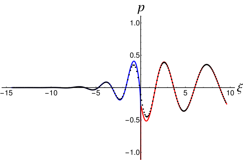
(a) The analytical solution excluding the immediate vicinity of the turning point (solid line) transitioning from an exponentially decaying solution to oscillatory is a combination of $p_{++}$ branch for $\Lambda<0$ (in blue), Eq. 38, and $p_{+-}$ branch for $\Lambda>0$ (in red), Eq. 37.

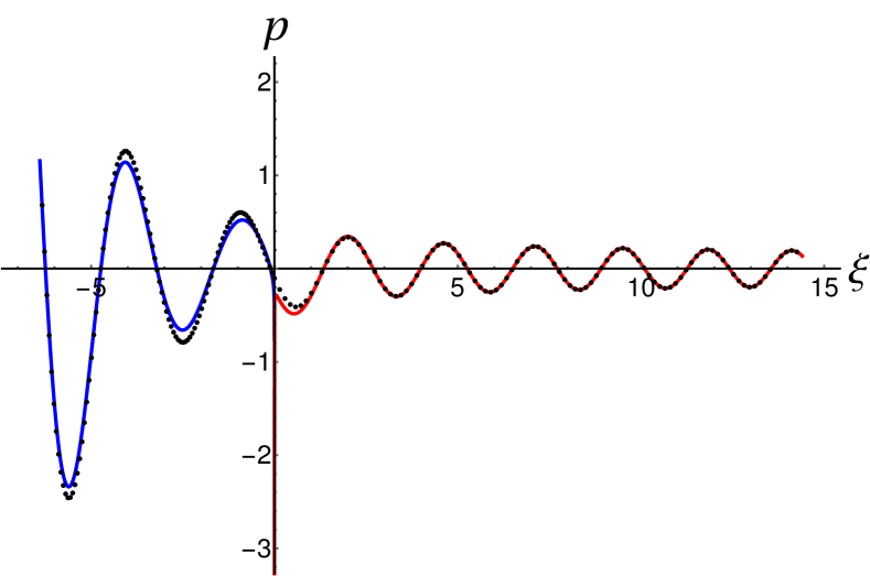
(b) The analytical solution excluding the immediate vicinity of the turning point (solid line) transitioning from an exponentially growing solution to oscillatory is a combination of $p_{+-}$ branch for $\Lambda<0$ (in blue), Eq. 39, and $p_{++}$ branch for $\Lambda>0$ (in red), Eq. 36.

Figure 16: Results of the numerical integration along the SDC contour shown as dots and the analytical estimates of the contour integral outside of the turning point as solid curves. Parameter values taken as $\rho=1/2^{4},~{}{\varepsilon}=1/2$ and hence, e.g., $\Lambda=0.9$ corresponds to $\xi=14.4$.

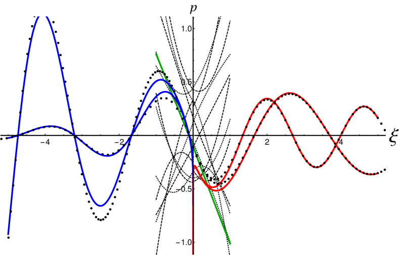
Figure 17: Contour integral asymptotics for $\rho=1/2^{4}$, ${\varepsilon}=1/2$ with the dots representing the numerically calculated contour integral along the SDC which allows us to calculate the behaviour even close to the turning point. Solid lines are the asymptotic approximations for the multiple contour integral solutions away from the transition point, Eqs. Eq. 36-Eq. 39 (note the blowup is outside of the range of validity). The black curves show all of the 12 potential approximations following from the analysis of coalescing saddles, Eq. 65. The match of the outer solution is remarkable except for a small neighbourhood of the turning point, where one of the calculated linear approximation works well (one for all four solutions). The correctly behaving root corresponds to the fifth root of $(-1)^{1/6}$ and the real part of $p$. The explicit expression is in the text, Eq. Eq. 43.

Solid lines are the asymptotics away from the transition point, Eqs. Eq. 36-Eq. 39 (note the blowup is outside of the range of validity and is not shown in Fig. 16). The black lines in Fig. 17 show all the 12 potential approximations following from the analysis of coalescing saddles, Eq. 65.

Note that the computations for $\Lambda<0$ and $\Lambda>0$ are quite different and so are the analytical expressions. Yet, the numerical solution seems to be smooth across the turning point $\Lambda=0$. In addition, the analytical results nicely match the numerics (and vice versa) with the notable exception being the vicinity of $\Lambda=0$.

Final form of solution near turning point

From the comparison of the numerical integration along the SDC contour, one can identify that the appropriate approximation (from the many contained in Eq. 65) corresponds to the real part of the fifth root of $(-1)^{1/6}$

(66) $$p \sim\frac{\pi\left(r^{\prime}(a)\right)^{1/3}}{6^{2/3}\Gamma(2/3)}\bigg{[}2\cos\left(\frac{8}{15r^{\prime}(a)}\right)+{r^{\prime}(a)^{1/2}}\bigg{(}\Theta(y)\sin\left(\frac{8}{15r^{\prime}(a)}\right)$$

$$-\Theta(-y)\cos\left(\frac{8}{15r^{\prime}(a)}\right)\bigg{)}\sqrt{|y|}+2\sin\left(\frac{8}{15r^{\prime}(a)}\right)y\bigg{]},$$

where $\Theta$ stands for the Heaviside step function. We verified this choice of the root on other random parameter sets and it always led to a visually correct approximation of the behaviour near the turning point, see Fig. 4. Note that the approximate solution is continuous but has a discontinuity in the first derivative (due to the Heaviside step function).

Thus the WKB solution, Eqs. Eq. 36-Eq. 39, shows excellent agreement with numerical integration up to a proximity to the turning point, where we have a linear approximation Eq. 43.

Note that this knowledge of the behaviour of the solutions reveals that the envelope is $\mathcal{O}\left(1\right)$ near the turning point; the leading order behaviour is actually a rescaled Airy function as follows from Eq (42)

(67) $$p\sim\underbrace{2\pi ie^{i\frac{1}{\varepsilon^{*}}\frac{8}{5}}(\varepsilon^{*})^{1/3}M_{-}}_{\mbox{constant}}\mathrm{Ai}\left((-i)^{3/2}(\varepsilon^{*})^{2/3}\Lambda(\xi)\right)$$

and hence the decay rates of the pattern tails correspond to the envelope behaviour of the Airy function matching those identified above in the outer WKB solution, Eqs. Eq. 36-Eq. 39.

Appendix B Numerical Methods

A complete copy of our numerical methods can be found in this GitHub repository. Briefly, we solve Eq. 1 using a standard finite difference discretization of the Laplacian, leading to a five-point stencil for the operator $(1+\varepsilon\nabla^{2})^{2}$ in MATLAB. The resulting system of time-dependent ordinary differential equations is evolved in time using the function ode15s, with a Jacobian sparsity pattern provided and absolute and relative tolerances set at $10^{-6}$. A minimum of $N=10,000$ grid points are used, though simulations for smaller $\varepsilon$ were checked for convergence using more grid points and finer time stepping tolerances. Initial conditions were set as independent and identically normally distributed random numbers for each grid point as $u(x,0)=\mathcal{N}(0,10^{-4})$. Simulations were run for $T=20,000$ units of time, and checked that they had reached an approximate steady state by evaluating the difference of solutions at time $t=10,000$ from the final time.

To help a reader explore these dynamics without having to use the code above, we have also implemented the model using VisualPDE [51] at this simulation link. This website provides a crude, yet rapid and interactive way to vary the parameters in the model and immediately observe the dynamics. The solution $u(x,t)$ is plotted in colour starting from small random initial data as described above, and the function $r(x)$ is plotted as a fixed black curve. The model implemented is of the form,

(68) $$\frac{\partial u}{\partial t}=r(x)u-\left(1+\varepsilon^{2}\frac{\partial^{2}}{\partial x^{2}}\right)^{2}u+au^{2}+bu^{3}+cu^{5},\quad\quad\quad x\in[0,1],$$

so one can easily observe supercritical dynamics by setting all of $a$,$b$, and $c$ to be non-positive, and subcritical dynamics by, e.g., setting $b>0$ and $c<0$ (as long as at least one higher-order nonlinearity is negative to ensure bounded solutions). Subcriticality can also be observed for $a>0$ for some values of $b$; see [11] for details in the case $c=0$. One can also modify the heterogeneity $r(x)$, and the value of $\varepsilon$. The default ranges provided should work without needing to change the time or space steps; modifying the system to be outside of these ranges, or using a different nonlinearity, are possible, but may require resolving the time and space step sizes to obtain well-behaved solutions. We would advise using this website only to get a rough picture of the dynamics, and to use the codes shared above via GitHub for a more accurate numerical treatment.

Finally, we remark that Fig. 6 was produced using the numerical continuation code BifurcationKit in the Julia language [50]. These BifurcationKit continuations were also used to check the direct method of continuation and computation of the energy $E(u^{*})$ which was done in MATLAB.

References

- [1] F. Al Saadi, A. Champneys, and N. Verschueren, Localized patterns and semi-strong interaction, a unifying framework for reaction–diffusion systems, IMA Journal of Applied Mathematics, 86 (2021), pp. 1031–1065.
- [2] R. A. Barrio, C. Varea, J. L. Aragón, and P. K. Maini, A two-dimensional numerical study of spatial pattern formation in interacting Turing systems, Bulletin of mathematical biology, 61 (1999), pp. 483–505.
- [3] M. Beck, J. Knobloch, D. J. Lloyd, B. Sandstede, and T. Wagenknecht, Snakes, ladders, and isolas of localized patterns, SIAM Journal on Mathematical Analysis, 41 (2009), pp. 936–972.
- [4] C. M. Bender and S. A. Orszag, Advanced mathematical methods for scientists and engineers I: Asymptotic methods and perturbation theory, Springer Science & Business Media, 2013.
- [5] D. L. Benson, P. K. Maini, and J. A. Sherratt, Unravelling the Turing bifurcation using spatially varying diffusion coefficients, Journal of Mathematical Biology, 37 (1998), pp. 381–417.
- [6] D. L. Benson, J. A. Sherratt, and P. K. Maini, Diffusion driven instability in an inhomogeneous domain, Bulletin of mathematical biology, 55 (1993), pp. 365–384.
- [7] J. J. Bramburger, D. J. Hill, and D. J. Lloyd, Localized multi-dimensional patterns, arXiv preprint arXiv:2404.14987, (2024).
- [8] V. brena Medina, A. R. Champneys, C. Grierson, and M. J. Ward, Mathematical modeling of plant root hair initiation: Dynamics of localized patches, SIAM Journal on Applied Dynamical Systems, 13 (2014), pp. 210–248.
- [9] V. F. brena Medina, D. Avitabile, A. R. Champneys, and M. J. Ward, Stripe to spot transition in a plant root hair initiation model, SIAM Journal on Applied Mathematics, 75 (2015), pp. 1090–1119.
- [10] J. Burke, S. Houghton, and E. Knobloch, Swift-hohenberg equation with broken reflection symmetry, Physical Review E—Statistical, Nonlinear, and Soft Matter Physics, 80 (2009), p. 036202.
- [11] J. Burke and E. Knobloch, Localized states in the generalized Swift-Hohenberg equation, Physical Review E—Statistical, Nonlinear, and Soft Matter Physics, 73 (2006), p. 056211.
- [12] J. Burke and E. Knobloch, Snakes and ladders: Localized states in the Swift–Hohenberg equation, Physics Letters A, 360 (2006), pp. 681–688.
- [13] E. A. Calderón-Barreto and J. L. Aragón, Turing patterns with space varying diffusion coefficients: Eigenfunctions satisfying the legendre equation, Chaos, Solitons & Fractals, 165 (2022), p. 112869.
- [14] S. Chapman and G. Kozyreff, Exponential asymptotics of localised patterns and snaking bifurcation diagrams, Physica D, 238 (2009), pp. 319–354.
- [15] C. Chester, B. Friedman, and F. Ursell, An extension of the method of steepest descents, in Mathematical Proceedings of the Cambridge Philosophical Society, vol. 53, Cambridge University Press, 1957, pp. 599–611.
- [16] D. L. Coelho, E. Vitral, J. Pontes, and N. Mangiavacchi, Stripe patterns orientation resulting from nonuniform forcings and other competitive effects in the swift–hohenberg dynamics, Physica D: Nonlinear Phenomena, 427 (2021), p. 133000.
- [17] M. P. Dalwadi and P. Pearce, Universal dynamics of biological pattern formation in spatio-temporal morphogen variations, Proceedings of the Royal Society A, 479 (2023), p. 20220829.
- [18] A. D. Dean, P. Matthews, S. Cox, and J. King, Exponential asymptotics of homoclinic snaking, Nonlinearity, 24 (2011), p. 3323.
- [19] E. A. Gaffney, A. L. Krause, P. K. Maini, and C. Wang, Spatial heterogeneity localizes Turing patterns in reaction-cross-diffusion systems, Discrete and Continuous Dynamical Systems-Series B, (2023).
- [20] D. J. Hill, The role of spatial dimension in the emergence of localised radial patterns from a turing instability, arXiv preprint arXiv:2405.16927, (2024).
- [21] T. W. Hiscock and S. G. Megason, Orientation of Turing-like patterns by morphogen gradients and tissue anisotropies, Cell systems, 1 (2015), pp. 408–416.
- [22] S. Houghton and E. Knobloch, Swift-hohenberg equation with broken cubic-quintic nonlinearity, Physical Review E—Statistical, Nonlinear, and Soft Matter Physics, 84 (2011), p. 016204.
- [23] F. Hummel, S. Jelbart, and C. Kuehn, Geometric blow-up of a dynamic turing instability in the swift-hohenberg equation, arXiv preprint arXiv:2207.03967, (2022).
- [24] D. Iron and M. J. Ward, Spike pinning for the gierer–meinhardt model, Mathematics and computers in simulation, 55 (2001), pp. 419–431.
- [25] H.-C. Kao, C. Beaume, and E. Knobloch, Spatial localization in heterogeneous systems, Physical Review E, 89 (2014), p. 012903.
- [26] E. Knobloch, Spatial localization in dissipative systems, Annual Review of Condensed Matter Physics, 6 (2015), pp. 325–359.
- [27] T. Kolokolnikov and J. Wei, Pattern formation in a reaction-diffusion system with space-dependent feed rate, SIAM Review, 60 (2018), pp. 626–645.
- [28] J. Kováč and V. Klika, Wkbj approximation for linearly coupled systems: asymptotics of reaction-diffusion systems, arXiv preprint arXiv:2104.09593, (2021).
- [29] J. Kováč and V. Klika, Liouville-green approximation for linearly coupled systems: Asymptotic analysis with applications to reaction-diffusion systems., Discrete & Continuous Dynamical Systems-Series S, 15 (2022).
- [30] A. L. Krause, E. A. Gaffney, T. J. Jewell, V. Klika, and B. J. Walker, Turing instabilities are not enough to ensure pattern formation, Bulletin of Mathematical Biology, 86 (2024), p. 21.
- [31] A. L. Krause, E. A. Gaffney, P. K. Maini, and V. Klika, Modern perspectives on near-equilibrium analysis of Turing systems, Philosophical Transactions of the Royal Society A: Mathematical, Physical and Engineering Sciences, 379 (2021).
- [32] A. L. Krause, V. Klika, T. E. Woolley, and E. A. Gaffney, Heterogeneity induces spatiotemporal oscillations in reaction-diffusion systems, Physical Review E, 97 (2018), p. 052206.
- [33] A. L. Krause, V. Klika, T. E. Woolley, and E. A. Gaffney, From one pattern into another: Analysis of Turing patterns in heterogeneous domains via WKBJ, Journal of the Royal Society Interface, 17 (2020), p. 20190621.
- [34] L. Lindblom and R. Robiscoe, Improving the accuracy of wkb eigenvalues, Journal of mathematical physics, 32 (1991), pp. 1254–1258.
- [35] E. Meron, Pattern-formation approach to modelling spatially extended ecosystems, Ecological Modelling, 234 (2012), pp. 70–82.
- [36] F. Olver, Asymptotics and special functions, AK Peters/CRC Press, 1997.
- [37] K. Onimaru, L. Marcon, M. Musy, M. Tanaka, and J. Sharpe, The fin-to-limb transition as the re-organization of a turing pattern, Nature communications, 7 (2016), p. 11582.
- [38] K. Page, P. K. Maini, and N. A. M. Monk, Pattern formation in spatially heterogeneous Turing reaction–diffusion models, Physica D: Nonlinear Phenomena, 181 (2003), pp. 80–101.
- [39] K. M. Page, P. K. Maini, and N. A. Monk, Complex pattern formation in reaction–diffusion systems with spatially varying parameters, Physica D: Nonlinear Phenomena, 202 (2005), pp. 95–115.
- [40] K. J. Painter, M. Ptashnyk, and D. J. Headon, Systems for intricate patterning of the vertebrate anatomy, Philosophical Transactions of the Royal Society A, 379 (2021), p. 20200270.
- [41] D. D. Patterson, A. C. Staver, S. A. Levin, and J. D. Touboul, Spatial dynamics with heterogeneity, SIAM journal on applied mathematics, (2023), pp. S225–S248.
- [42] J. Raspopovic, L. Marcon, L. Russo, and J. Sharpe, Digit patterning is controlled by a bmp-sox9-wnt turing network modulated by morphogen gradients, Science, 345 (2014), pp. 566–570.
- [43] P. Rohani, T. J. Lewis, D. Grünbaum, and G. D. Ruxton, Spatial self-organisation in ecology: pretty patterns or robust reality?, Trends in Ecology & Evolution, 12 (1997), pp. 70–74.
- [44] A. Scheel and J. Weinburd, Wavenumber selection via spatial parameter jump, Philosophical Transactions of the Royal Society A: Mathematical, Physical and Engineering Sciences, 376 (2018), p. 20170191.
- [45] N. M. Temme, Asymptotic methods for integrals, vol. 6, World Scientific, 2014.
- [46] A. M. Turing, The chemical basis of morphogenesis, Philosophical Transactions of the Royal Society of London. Series B, Biological Sciences, 237 (1952), pp. 37–72.
- [47] H. Uecker, Pattern formation with pde2path–a tutorial, arXiv preprint arXiv:1908.05211, (2019).
- [48] R. A. Van Gorder, Pattern formation from spatially heterogeneous reaction–diffusion systems, Philosophical Transactions of the Royal Society A, 379 (2021), p. 20210001.
- [49] J. C. Vandenberg and M. B. Flegg, Turing pattern or system heterogeneity? A numerical continuation approach to assessing the role of Turing instabilities in heterogeneous reaction-diffusion systems, arXiv preprint arXiv:2301.08373, (2023).
- [50] R. Veltz, BifurcationKit.jl, July 2020, https://hal.archives-ouvertes.fr/hal-02902346.
- [51] B. J. Walker, A. K. Townsend, A. K. Chudasama, and A. L. Krause, VisualPDE: rapid interactive simulations of partial differential equations, Bulletin of Mathematical Biology, 85 (2023), p. 113.
- [52] P. Woods and A. Champneys, Heteroclinic tangles and homoclinic snaking in the unfolding of a degenerate reversible Hamiltonian–Hopf bifurcation, Physica D: Nonlinear Phenomena, 129 (1999), pp. 147–170.
- [53] T. E. Woolley, A. L. Krause, and E. A. Gaffney, Bespoke Turing systems, Bulletin of Mathematical Biology, 83 (2021), pp. 1–32.