Shape and energy of a membrane on a liquid interface with arbitrary curvatures

Abstract

We study the deformation of a liquid interface with arbitrary principal curvatures by a flat circular sheet. We use the membrane limit, where the sheet is inextensible yet free to bend and compress, and restrict ourselves to small slopes. We find that the sheet takes a cylindrical shape on interfaces with negative Gaussian curvature. On interfaces with positive Gaussian curvature, an inner region still adopts a cylindrical shape while the outer region is under azimuthal compression. Our predictions are confirmed by numerical energy minimization. Finally, we compute the energy of placing the sheet on the curved interface and find that it is much lower for positive Gaussian curvatures than for negative ones, that is, peaks and valleys are covered more efficiently than saddles.

Experiments where a thin elastic solid is placed on a surface with a different metric can reveal how a physical system grapples with the basic mathematical conflict of two incompatible metrics [1, 2]. One avenue for studying these problems has been to stamp [3, 4] or adhere [5, 6, 7] a sheet onto a curved substrate, thereby forcing the sheet to adopt a wrinkle pattern that approximates the confining geometry. In some cases, a liquid surface can provide such strong confinement, for instance when a thin curved shell is laid on a flat liquid bath [8, 9, 10]. In other cases, a shell can impose its own metric on a droplet [11], a response termed “sculpting”. Lying between these two extremes, both the liquid and the sheet can deform into a non-trivial shape that matches neither of the original geometries [12, 13, 14, 15].

While much has been elucidated about the behavior of a thin sheet confined to a liquid interface, the vast majority of these studies were carried out in axisymmetric configurations, leaving the case with different principal curvatures $\kappa_{x}$ and $\kappa_{y}$, as shown in Fig. 1, unexplored. For the case of solid confinement, previous work has focused on the role of the Gaussian curvature, $K=\kappa_{x}\kappa_{y}$, at driving the film response [3, 5]. For instance, in stamping or adhesion, the deformation of the sheet is primarily controlled by the difference between the Gaussian curvature of the sheet $K_{\mathrm{sh}}$ and that of the solid substrate, $K_{\mathrm{sub}}$ [3, 16, 4, 7]. This result extends to a shell confined to a flat liquid, as gravity prevents large deformations [8, 11, 9, 10]. However, whether this result generally applies to liquid interfaces remains unclear.

Here, we study this problem using the simplest theoretical model: the sheet is treated as an inextensible, highly flexible membrane that can compress and wrinkle freely [13, 17] and we work in the limit of small slopes. We predict the resulting shape of the sheet and liquid interfaces, along with the energies associated with covering liquids of different geometries, which are in good agreement with our numerical energy minimizations in Surface Evolver [18]. For both positive and negative Gaussian curvatures, there is a region of the sheet which forms a cylindrical shape where the sheet only curves along a single principle axis [Fig. 2(a,b)]. We find that the deformations are not controlled solely by the Gaussian curvature, but instead by the mean curvature and the difference between $\kappa_{x}$ and $\kappa_{y}$. These results comprise a fundamentally different response from related studies with other forms of confinement [3, 5, 16, 8, 4, 9, 10, 7].

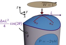
Figure 1: Setup: a flat circular sheet with radius $W=1$ is placed on a liquid interface with principal curvatures $\kappa_{x}$ and $\kappa_{y}$. The curvature difference $\Delta\kappa=\kappa_{x}-\kappa_{y}$ is set by the shape of the edge while the mean curvature $H=(\kappa_{x}+\kappa_{y})/2$ is set by the pressure applied under the interface.

A liquid interface with arbitrary curvatures can be formed by pinning its edge at a frame with radius $L$ and height $\zeta(L,\theta)=\Delta\kappa L^{2}\cos(2\theta)/4$ and applying a pressure $P=-2\gamma H$ under the interface (Fig. 1), where $\gamma$ is the surface tension of the interface. We assume that the vertical extension of the interface, scaling as $\kappa_{i}L^{2}$, is small with respect to the capillary length, so that the effect of gravity is negligible. Last, we restrict ourselves to small slopes. Under these conditions, the height of the liquid interface reads, in polar coordinates (App. A.1):

$$\zeta_{0}(r,\theta)=\frac{H}{2}(r^{2}-L^{2})+\frac{\Delta\kappa}{4}r^{2}\cos(2\theta),$$ (1)

where $H$ and $\Delta\kappa$ are related to the principal curvatures $\kappa_{x}$ and $\kappa_{y}$ by $H=(\kappa_{x}+\kappa_{y})/2$ and $\Delta\kappa=\kappa_{x}-\kappa_{y}$. We choose $x$ as the most curved direction, $\kappa_{x}>|\kappa_{y}|$.

We then place a circular inextensible sheet with radius $W<L$ at the center of the interface (we now use $W$ as the unit length). The sheet is treated as inextensible but with zero bending modulus; such a membrane strongly resists in-plane stretching while being free to wrinkle and deform under minute compressive stresses; such small-scale wrinkling can allow lengths in the sheet to effectively shorten [19, 13, 17]. With the sheet, the shape of the liquid interface ($r\geq 1$) is perturbed and takes the form (App. A.2)

$$\zeta(r,\theta)=\frac{H}{2}(r^{2}-L^{2})+\left(ar^{2}+\frac{b}{r^{2}}\right)\cos(2\theta).$$ (2)

We assume a vertical displacement of the sheet ($r\leq 1$) of the form

$$\zeta(r,\theta)=c_{2}(r)\cos(2\theta)+c_{0}(r).$$ (3)

Matching the general shape (2) with the boundary conditions at $r=1$ and $r=L$ gives

$$a =\frac{\frac{1}{4}\Delta\kappa L^{4}-c_{2}(1)}{L^{4}-1},$$ (4)

$$b =\frac{c_{2}(1)-\frac{1}{4}\Delta\kappa}{1-L^{-4}}.$$ (5)

We use force balance to determine the shape of the sheet. We start with the case where the edge of the sheet is under radial tension and azimuthal compression: the radial strain $\epsilon_{rr}$ vanishes, and only the radial component of the stress $\sigma_{rr}$ is nonzero. The in-plane force balance gives $\partial_{r}(r\sigma_{rr})=0$, hence $\sigma_{rr}(r)=\gamma/r$ due to the boundary condition $\sigma_{rr}(1)=\gamma$ (App. B.1).

We now use the out-of-plane force balance: $\sigma_{rr}(r)\partial_{r}^{2}\zeta(r,\theta)=2\gamma H$. Using the vertical displacement (3) and the radial stress $\sigma_{rr}(r)=\gamma/r$, it reads $\partial_{r}^{2}\zeta(r,\theta)=c_{2}^{\prime\prime}(r)\cos(2\theta)+c_{0}^{\prime\prime}(r)=2Hr$, leading to $c_{2}^{\prime\prime}(r)=0$ and $c_{0}^{\prime\prime}(r)=2Hr$. Moreover, the height and the slope should be continuous at the edge of the sheet, meaning that $\zeta(1,\theta)=c_{2}(1)\cos(2\theta)+c_{0}(1)=(a+b)\cos(2\theta)+\frac{H}{2}(1-L^{2})$, and $\partial_{r}\zeta(1,\theta)=c_{2}^{\prime}(1)\cos(2\theta)+c_{0}^{\prime}(1)=2(a-b)\cos(2\theta)+H$, where $a$ and $b$ are given by Eqs. (4, 5). Together, this leads to

$$c_{0}^{\prime}(r) =Hr^{2},$$ (6)

$$c_{2}(r) =2(a-b)r-a+3b.$$ (7)

Unless $a=b=0$, these expressions cannot hold down to the center of the sheet as there would be a singularity at the origin. The slope along $y$, $c_{0}^{\prime}(r)-c_{2}^{\prime}(r)$ reaches $0$ at $r=\ell$ where $H\ell^{2}=2(a-b)$, pointing to a cylindrical shape. We thus assume that the shape is cylindrical for $r\leq\ell$, meaning that $c_{0}^{\prime}(r)=c_{2}^{\prime}(r)=H\ell r$: the sheet is curved only in the $x$ direction, with curvature $\kappa_{x}=2H\ell$. To balance the pressure the stress should be $\sigma_{xx}=2\gamma H/\kappa_{x}=\gamma/\ell$, consistent with $\sigma_{rr}(\ell)=\gamma/\ell$. The boundary condition for the stress also imposes $\sigma_{yy}=\gamma/\ell$: for $r\leq\ell$, the sheet is under tension in all directions with an isotropic stress $\gamma/\ell$. Finally, the position $\ell$ can be determined by using the continuity of the height and slope at $r=\ell$ together with the relations (4, 5), leading to (App. B.2)

$$\ell^{2}\left(3-\ell+\frac{1-\ell}{L^{4}}\right)=\frac{\Delta\kappa}{H}=\frac{2(\kappa_{x}-\kappa_{y})}{\kappa_{x}+\kappa_{y}},$$ (8)

This equation admits a solution in the range $[0,1]$ for $\Delta\kappa/H$ in the range $[0,2]$, corresponding to $\kappa_{y}$ in the range $[0,\kappa_{x}]$ (Fig. 2(f)). As expected $\ell=0$ in the axisymmetric case $\kappa_{y}=\kappa_{x}$ and $\ell=1$ in the cylindrical case $\kappa_{y}=0$. A representation of the predicted shape for $0<\kappa_{y}<\kappa_{x}$ is shown in Fig. 2(a).

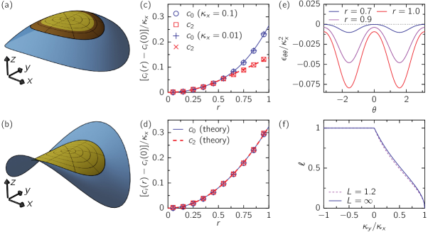
Figure 2: (a,b) Rendering of the shapes predicted for $\kappa_{y}=\kappa_{x}/2$ and $\kappa_{y}=-\kappa_{x}/2$, respectively. The shape is cylindrical in the yellow region. (c, d) values of $c_{0}(r)$ and $c_{2}(r)$ obtained from the fits (circles) and theoretical predictions (solid lines) for $\kappa_{y}=\kappa_{x}/2$ and $\kappa_{y}=-\kappa_{x}/2$, respectively, for $L=1.2$. (e) Azimuthal strain at different radii $r_{i}>\ell\simeq 0.52$ indicated in the graph key for $\kappa_{y}=\kappa_{x}/2$. (f) Extension of the cylindrical region $\ell$ as a function of the ratio of the curvatures, for $L=1.2$ (dashed line) and $L=\infty$ (solid line).

Based on the calculation above, we assume that the shape remains cylindrical for $\kappa_{y}<0$: $c_{0}(r)=Cr^{2}+c_{0}(0)$, $c_{2}(r)=Cr^{2}$. The edge being under azimuthal tension, it can carry a stress; moreover, since the sheet is inextensible, the stress can be localized at the edge, we denote this singular part $\hat{\sigma}_{\theta\theta}(r)=\Sigma\delta(r-1)$. This singular azimuthal stress can give rise to a stress jump in the longitudinal direction, as can be seen from the in-plane force balance $\partial_{r}[r\sigma_{rr}(r)]=\sigma_{\theta\theta}(r)$, leading to

$$\sigma_{rr}(1^{-})=\gamma-\Sigma.$$ (9)

The singular azimuthal stress also allows a slope discontinuity at the interface, which is given by the out-of-plane force balance (App. B.3):

$$\gamma\partial_{r}\zeta(1^{+},\theta)-\sigma_{rr}(1^{-})\partial_{r}\zeta(1^{-},\theta)+\Sigma\partial_{\theta}^{2}\zeta(1,\theta)=0.$$ (10)

Combining these equations with (4, 5), we can determine the shape of the sheet and the singular edge stress (App. B.4):

$$C =\frac{(1-L^{-4})H+\Delta\kappa}{6-2L^{-4}}.$$ (11)

$$\frac{\Sigma}{\gamma} =1-\frac{H}{2C}=1-\frac{(3-L^{-4})H}{(1-L^{-4})H+\Delta\kappa}.$$ (12)

The edge stress should be positive, which is the case for $2H\leq\Delta\kappa$, or $\kappa_{y}\leq 0$, as expected. Renderings of the predicted shapes are shown in Fig. 2 for $\kappa_{y}=\pm\kappa_{x}/2$. A representation of the predicted shape for $-\kappa_{x}<\kappa_{y}<0$ is shown in Fig. 2(b).

We compare our theoretical predictions to numerical energy minimization using “Surface Evolver” (App. C) [18] . We allow mesh edges within the sheet to shorten at zero cost, to capture the effect of small-amplitude, short-wavelength wrinkles that can form in the sheet. The sheet nevertheless resists stretching, which we implement using a large stretching modulus, $Y=10^{12}\gamma$. First, we check that the shape is of the form (3) by plotting the vertical displacement over a narrow annulus; the functions $c_{i}(r)$ are then obtained by fitting the angular dependence at different radii (App. C). The results are compared to the predictions for several values of $\kappa_{x}$ and $\kappa_{y}=\pm\kappa_{x}/2$ in Fig. 2(c,d); a very good agreement is obtained.

To better understand how the sheet accommodates its inextensibility constraint, we compute the in-plane displacements $u_{r}(r,\theta)$ and $u_{\theta}(r,\theta)$ associated with the vertical displacement $\zeta(r,\theta)$ (App. D). This allows us to obtain the azimuthal compression $\epsilon_{\theta\theta}(r,\theta)$ in the outer annulus $r>\ell$; it is shown in Fig. 2(e) for $\kappa_{y}=\kappa_{x}/2$ for different values of $r$. We find that the azimuthal strain is compressive everywhere for $r>\ell$, albeit with a strong angular dependence, and that it vanishes at $r=\ell$, as expected.

Finally, the in-plane displacement gives access to the energy of the system, which consists of two terms: the interfacial energy and the potential energy associated to the pressure. The interfacial energy is affected by the deformation of the interface caused by the sheet and by the inward motion of the edge of the sheet, encoded in the radial in-plane displacement $u_{r}(r,\theta)$. The potential energy is affected by the volume of liquid beneath the sheet. Taking into account these contributions, the difference between the energy gain obtained by placing the sheet on a flat interface and the one obtained by placing the sheet on a doubly curved interface is (App. E)

$$\frac{\Delta U}{\pi\gamma}=\frac{H^{2}}{4}+\frac{\Delta\kappa^{2}}{8(1-L^{-4})}-2H\int_{0}^{1}r^{2}c_{0}^{\prime}(r)\mathrm{d}r\\ +\frac{L^{4}+1}{L^{4}-1}c_{2}(1)^{2}-\frac{\Delta\kappa c_{2}(1)}{1-L^{-4}}-2a_{0}(1),$$ (13)

where $a_{0}(r)$ is the angular average of $u_{r}(r,\theta)$. The energy can be obtained by inserting the predicted shape in this expression; it is shown in Fig. 3. A strong asymmetry is observed: for a given absolute value of Gaussian curvature, the energy is larger when the Gaussian curvature is negative, meaning that the sheet covers more efficiently peaks and valleys than saddles. Interestingly, in the limit $L\to\infty$, the energy for a negative Gaussian curvature is $\Delta U/(\pi\gamma)=\kappa_{y}^{2}/6$: the energy is controlled by the weakest curvature.

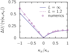
Figure 3: Energy gain of placing the sheet on a curved interface minus the energy gain of placing the sheet of a flat interface, normalized by the absolute value of the Gaussian curvature as a function of the ratio of curvatures for $L=1.2$ (dashed line) and $L=\infty$ (solid line).

Symmetry allows to deduce the shape of the sheet for arbitrary curvatures from the calculations in the case where $\kappa_{x}=|\kappa_{y}|$. While the situation where $\kappa_{x}=\kappa_{y}$ is the axisymmetric case, whose solution is the parachute shape predicted by Taylor [20], the case with $\kappa_{x}=-\kappa_{y}$, hence with zero mean curvature $H$, should be treated carefully. Indeed, our prediction is that for negative Gaussian curvatures the sheet adopts a cylindrical shape which is flat in the less curved direction of the interface. As a consequence, the flat direction changes abruptly when $\kappa_{y}$ crosses $-\kappa_{x}$. At the transition, where $\kappa_{x}=-\kappa_{y}$, the sheet is floppy and there are many configurations that minimize the energy. This is due to the fact that the pressure across the interface, which is proportional to the mean curvature, is zero.

Our results have been obtained under two approximations. One is the membrane limit, which assumes that the sheet is inextensible yet free to bend. Imparting a finite cost to bending would make the problem much more complicated by bringing in an energy scale associated with the curvature of the sheet. Such resistance to bending is relevant for “thick” sheets, of the order of tens of micrometers [21]. On the other hand, the small but finite extensibility of “thin” sheets, of the order of a hundred nanometers, is clearly visible in experiments where a flat sheet is placed on a curved droplet [12] and where a curved shell is placed on a flat interface [11]. The sheets in these experiments would be fully wrinkled if they were inextensible; instead they display some unwrinkled regions where the sheet is stretched. For positive Gaussian curvatures, the extent of the unwrinkled region in the center of the sheet determined in Ref. [12] should be compared with the extent $\ell$ of the cylindrical region. For negative Gaussian curvatures, the edge stress that we predict would extend over a finite annulus [11] and the shape would be cylindrical in the inner region.

The second assumption is the restriction to small slopes. Going beyond is a considerable challenge for mainly two reasons. First, there is no interface with constant mean and Gaussian curvatures, so that the very question that we ask and answer here should be modified. Second, even in the simplest, axisymmetric situation where $\kappa_{x}=\kappa_{y}$, the sheet breaks axisymmetry and no analytical solution is known [13].

Under the approximations that we have used, we have found that the sheet adopts a cylindrical shape when placed on a liquid interface with negative Gaussian curvature. In this situation, the sheet retains its metric and imposes it to the interface: it “sculpts” the interface, as a thin shell placed on a curved interface [11]. There is a slight difference between the two cases: here, the sheet retains its metric but not its shape, contrary to the situation in Ref. [11], so that the sculpting is weaker here; this is due to the fact that there are more embeddings of the flat metric compared to the spherical one [22]. When the Gaussian curvature of the interface is positive, the sheet still adopts a cylindrical shape in its center, and thus partially sculpts the interface. The “rim” that connects the sculpted region to the liquid interface is here purely geometric, while the one observed in Ref. [11] is due to the finite extensibility of the sheet. Finally, we note that whether the sheet is flat or spherical, sculpting may occur when the Gaussian curvature of the sheet is larger than that of the interface. Hence, while the precise response of the sheet does not depend solely on the Gaussian curvature mismatch, some aspects of the sheet-interface interaction seem to be determined by the sign of the mismatch. In order to verify it, one would have to determine the shape of a sheet with arbitrary curvatures placed on an arbitrary liquid interface.

Appendix A Liquid interface

A.1 Bare liquid interface

A.1.1 Shape

We start by determining the height $\zeta(r,\theta)$ of the liquid interface without sheet. It should minimize the energy

$$U=\gamma A-PV=\gamma(A+2HV),$$ (14)

where $A$ is the area of the liquid interface and $V$ the volume of liquid contained below it:

$$A =\int\sqrt{1+[\nabla\zeta(\boldsymbol{r})]^{2}}\mathrm{d}\boldsymbol{r}\simeq\pi L^{2}+\frac{1}{2}\int[\nabla\zeta(\boldsymbol{r})]^{2}\mathrm{d}\boldsymbol{r},$$ (15)

$$V =\int\zeta(\boldsymbol{r})\mathrm{d}\boldsymbol{r},$$ (16)

where the integrals run over the disc of radius $L$, and the second equality in Eq. (15) corresponds to the small slope limit. The interface should also satisfy the boundary condition

$$\zeta(L,\theta)=\frac{\Delta\kappa}{4}L^{2}\cos(2\theta).$$ (17)

Minimizing the energy (14) under the small slope limit leads to

$$\nabla^{2}\zeta(\boldsymbol{r})=2H.$$ (18)

Solving this equation with the boundary condition (17) gives the height field

$$\zeta(r,\theta) =\frac{H}{2}(r^{2}-L^{2})+\frac{\Delta\kappa}{4}r^{2}\cos(2\theta)$$ (19)

$$=\frac{\kappa_{1}}{2}x^{2}+\frac{\kappa_{2}}{2}y^{2},$$ (20)

where $\kappa_{1}$ and $\kappa_{2}$ are the principal curvatures and

$$H =\frac{\kappa_{1}+\kappa_{2}}{2},$$ (21)

$$\Delta\kappa =\kappa_{1}-\kappa_{2}.$$ (22)

A.1.2 Energy

The energy of the interface is

$$\frac{U}{\pi\gamma}=L^{2}-\frac{H^{2}L^{4}}{4}+\frac{\Delta\kappa^{2}L^{4}}{16}.$$ (23)

A.2 Liquid interface deformed by the sheet

A.2.1 Shape

The sheet may perturb the liquid interface for $r>W=1$. This perturbation should not affect the mean curvature of the interface; we also assume that it has the same symmetry as the bare interface. We thus look for a height of the form

$$\zeta(r,\theta)=\frac{H}{2}(r^{2}-L^{2})+\left(ar^{2}+\frac{b}{r^{2}}\right)\cos(2\theta).$$ (24)

The parameters $a$ and $b$ are determined by the boundary condition (Eq. (17)), and the height of the edge of the sheet $C_{2}=c_{2}(1)$,

$$\zeta(1,\theta)=\frac{H}{2}(1-L^{2})+C_{2}\cos(2\theta).$$ (25)

Matching the general shape (24) with the boundary conditions (17, 25) gives

$$a =\frac{\frac{1}{4}\Delta\kappa L^{4}-C_{2}}{L^{4}-1},$$ (26)

$$b =\frac{C_{2}-\frac{1}{4}\Delta\kappa}{1-L^{-4}}.$$ (27)

A.2.2 Energy

The area is given by

$$A_{\mathrm{i}} =\pi(L^{2}-1)+\frac{1}{2}\int_{1<r<L}(\nabla\zeta)^{2}\mathrm{d}\boldsymbol{r}$$ (28)

$$=\pi(L^{2}-1)+\frac{1}{2}\int_{1<r<L}\left([\partial_{r}\zeta(r,\theta)]^{2}+r^{-2}[\partial_{\theta}\zeta(r,\theta)]^{2}\right)r\mathrm{d}r\mathrm{d}\theta$$ (29)

$$=\pi(L^{2}-1)+\frac{\pi H^{2}}{4}(L^{4}-1)+\pi(L^{4}-1)\left(a^{2}+\frac{b^{2}}{L^{4}}\right)$$ (30)

$$=\pi(L^{2}-1)+\frac{\pi H^{2}}{4}(L^{4}-1)+\pi\left[\frac{\left(C_{2}-\frac{1}{4}\Delta\kappa L^{4}\right)^{2}}{L^{4}-1}+\frac{1}{1-L^{-4}}\left(C_{2}-\frac{\Delta\kappa}{4}\right)^{2}\right].$$ (31)

The anisotropic term does not affect the volume of liquid below the interface, which is given by

$$V_{\mathrm{i}}=-\frac{\pi H}{4}(L^{4}-2L^{2}+1).$$ (32)

The energy of the interface is thus given by

$$\frac{U_{\mathrm{i}}}{\pi\gamma}=L^{2}-1+\frac{H^{2}}{4}(-L^{4}+4L^{2}-3)+\frac{\left(C_{2}-\frac{1}{4}\Delta\kappa L^{4}\right)^{2}}{L^{4}-1}+\frac{1}{1-L^{-4}}\left(C_{2}-\frac{\Delta\kappa}{4}\right)^{2}.$$ (33)

The difference with the energy of the bare interface (Eq. (23)) is

$$\frac{\Delta U}{\pi\gamma}=-1+\frac{H^{2}}{4}(4L^{2}-3)+\frac{L^{4}+1}{L^{4}-1}C_{2}^{2}-\frac{\Delta\kappa C_{2}}{1-L^{-4}}+\frac{\Delta\kappa^{2}}{8(1-L^{-4})}.$$ (34)

Appendix B Force balance

B.1 In-plane and out-of-plane force balance

We start by recalling the force balance equations for zero bending modulus ($B=0$) and in the absence of shear stress ($\sigma_{r\theta}=0$). The in-plane and out-of-plane read, respectively [12],

$$\partial_{r}(r\sigma_{rr}) =\sigma_{\theta\theta},$$ (35)

$$\sigma_{rr}\partial_{r}^{2}\zeta+\frac{1}{r^{2}}\sigma_{\theta\theta}\left(\partial_{\theta}^{2}\zeta+r\partial_{r}\zeta\right) =-P.$$ (36)

B.2 Size of the cylindrical region

We have seen in the main text that the slope along $y$ cancels at a radius $\ell$ where $H\ell^{2}/2=a-b$, and that assuming a cylindrical shape for $r<\ell$ leads to $c_{0}^{\prime}(r)=c_{2}^{\prime}(r)=H\ell r$. Since continuity of the height at $r=0$ requires $c_{2}(0)=0$, we can integrate $c_{2}^{\prime}(r)$ to obtain $c_{2}(r)=H\ell r^{2}/2$. The continuity of $c_{2}(r)$ at $r=\ell$ gives $H\ell^{3}/2=2(a-b)\ell-a+3b$. Taking into account the fact that $a-b=H\ell^{2}/2$, we end up with $H\ell^{3}/2=a-3b$. Finally, there are two equations relating $a$ and $b$ to $H$ and $\ell$:

$$a-b =\frac{H\ell^{2}}{2},$$ (37)

$$a-3b =\frac{H\ell^{3}}{2}.$$ (38)

Solving for $a$ and $b$, we find

$$a =\frac{H}{4}\ell^{2}(3-\ell),$$ (39)

$$b =\frac{H}{4}\ell^{2}(1-\ell).$$ (40)

The boundary condition at $r=L$, imposes $aL^{2}+bL^{-2}=\Delta\kappa L^{2}/4$. Inserting the expressions of $a$ and $b$ in this equation, we obtain

$$\ell^{2}\left[3-\ell+\frac{1-\ell}{L^{4}}\right]=\frac{\Delta\kappa}{H}.$$ (41)

which is the equation that determines $\ell$.

B.3 Slope discontinuity in the presence of a singular edge stress

To determine the equation for the slope discontinuity at the edge, we start from the out-of-plane force balance (36), which we multiply by $r$ and expand:

$$r\sigma_{rr}\partial_{r}^{2}\zeta+\sigma_{\theta\theta}\partial_{r}\zeta+\frac{1}{r}\sigma_{\theta\theta}\partial_{\theta}^{2}\zeta=-Pr.$$ (42)

Now using the in-plane force balance (35) in the second term, we obtain

$$r\sigma_{rr}\partial_{r}^{2}\zeta+\partial_{r}(r\sigma_{rr})\partial_{r}\zeta+\frac{1}{r}\sigma_{\theta\theta}\partial_{\theta}^{2}\zeta=-Pr,$$ (43)

so that the first two terms correspond to a derivative,

$$\partial_{r}\left(r\sigma_{rr}\partial_{r}\zeta\right)+\frac{1}{r}\sigma_{\theta\theta}\partial_{\theta}^{2}\zeta=-Pr,$$ (44)

Integrating the last relation between $1^{-}$ and $1^{+}$ leads to

$$\gamma\partial_{r}\zeta(1^{+},\theta)-\sigma_{rr}(1^{-})\partial_{r}\zeta(1^{-},\theta)+\Sigma\partial_{\theta}^{2}\zeta(1,\theta)=0,$$ (45)

which is the equation given in the main text.

B.4 Parameters of the cylindrical shape

With the assumed shape for the sheet, we have $\partial_{r}\zeta(1^{-},\theta)=2C[1+\cos(2\theta)]$ and $\partial_{\theta}^{2}\zeta(1,\theta)=-4C\cos(2\theta)$. For the liquid interface (Eq. (24)), $\partial_{r}\zeta(1^{+},\theta)=H+2(a-b)\cos(2\theta)$. Separating the $\theta$ independent and $\cos(2\theta)$ contributions in the out-of-plane force balance (45), we get

$$\gamma H-2(\gamma-\Sigma)C =0,$$ (46)

$$2\gamma(a-b)-2(\gamma-\Sigma)C-4\Sigma C =0.$$ (47)

The first equation gives

$$\frac{\Sigma}{\gamma}=1-\frac{H}{2C}.$$ (48)

Moreover, the continuity of the height implies $C=a+b$. Combining the equations above leads to

$$a =\frac{3\Delta\kappa-2L^{-4}H}{12(1-\frac{1}{3}L^{-4})},$$ (49)

$$b =\frac{2H-\Delta\kappa}{12(1-\frac{1}{3}L^{-4})},$$ (50)

$$C =a+b=\frac{(1-L^{-4})H+\Delta\kappa}{6(1-\frac{1}{3}L^{-4})}.$$ (51)

Appendix C Numerical energy minimization with Surface Evolver

We translate our membrane model into a computational model, using the “Surface Evolver” software [18], where the system consists of a sheet attached to a liquid interface. We use a triangulated surface (Fig. 4) with a mesh size of $0.1$. The liquid has surface tension $\gamma=1$ and the sheet is a disc of radius $W=1$. The sheet has a bending modulus of zero to allow it to bend freely. In-plane sheet deformations are realized via an asymmetric elasticity: the compressive energy cost between points is zero, while points stretching past their initially prescribed distance is highly discouraged by using a large stretch modulus ($10^{12}$). The boundary radius is fixed at $L=1.2$ and the boundary height and pressure are specified to achieve the desired curvature for each simulation. Starting at a stretching modulus of 10, we minimize the system energy using the conjugate gradient algorithm. We then increase the stretching modulus by a factor of $10^{0.001}$ and relax the system again (this factor yields 1000 evenly spaced steps for each order of magnitude of the stretch modulus). This sequence is repeated until the stretch modulus is at the desired value.

The height of an annulus around a radius $r$ can be fit with a heigth function of the form (Eq. (3) in the main text)

$$\zeta(r,\theta)=c_{2}(r)\cos(2\theta)+c_{0}(r),$$ (52)

giving the values of $c_{2}(r)$ and $c_{0}(r)$ (Fig. 5).

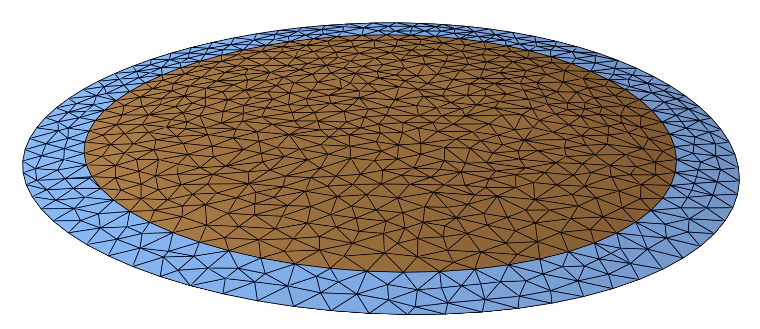
Figure 4: Rendering of the final configuration obtained by energy numerical energy minimization with the mesh represented as black segments. Parameters are $L=1.2$, $\kappa_{1}=0.1$, $\kappa_{2}=0.05$.

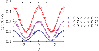
Figure 5: Vertical displacement as a function of the angle for different annuli, Surface Evolver simulations (circles) and fit with Eq. (52) (solid lines). Parameters are $L=1.2$, $\kappa_{1}=0.1$, $\kappa_{2}=0.05$.

Appendix D In-plane displacement and strain

D.1 General expressions

We denote $r$ and $\theta$ the material polar coordinates and $u_{r}(s,\theta)$, $u_{\theta}(s,\theta)$ and $\zeta(s,\theta)$ the radial, orthoradial and vertical displacements (out of plane), respectively.

The rest configuration of the sheet is given by

$$\boldsymbol{X}_{0}(r,\theta)=\begin{pmatrix}r\cos(\theta)\\ r\sin(\theta)\\ 0\end{pmatrix}.$$ (53)

The metric is given by

$$g_{0}=\partial_{i}\boldsymbol{X}\cdot\partial_{j}\boldsymbol{X}=\begin{pmatrix}1&0\\ 0&r^{2}\end{pmatrix}.$$ (54)

The deformed configuration is given by

$$\boldsymbol{X}(s,\theta)=\begin{pmatrix}(s+u_{r})\cos(\theta)-u_{\theta}\sin(\theta)\\ (s+u_{r})\sin(\theta)+u_{\theta}\cos(\theta)\\ \zeta\end{pmatrix}.$$ (55)

To compute the metric $g$ in the deformed configuration and deduce the strain $\epsilon$, we restrict ourselves to the lowest order in the displacements: order 1 for the in-plane displacements $u_{r}$ and $u_{\theta}$, order 2 for the out-of-plane displacement $\zeta$. We find

$$\epsilon=\frac{g-g_{0}}{2}=\begin{pmatrix}\partial_{r}u_{r}+\frac{1}{2}(\partial_{r}\zeta)^{2}&\frac{1}{2}[-u_{\theta}+\partial_{\theta}u_{r}+r\partial_{r}u_{\theta}+(\partial_{r}\zeta)(\partial_{\theta}\zeta)]\\ \frac{1}{2}[-u_{\theta}+\partial_{\theta}u_{r}+r\partial_{r}u_{\theta}+(\partial_{r}\zeta)(\partial_{\theta}\zeta)]&r(u_{r}+\partial_{\theta}u_{\theta})+\frac{1}{2}(\partial_{\theta}\zeta)^{2}\end{pmatrix}$$ (56)

The derivatives with respect to $r$ and $\theta$ having different dimensions, the different components of the strain have different dimensions. The physical strain is

$$\tilde{\epsilon}=g_{0}^{-1/2}\epsilon g_{0}^{-1/2}=\begin{pmatrix}\partial_{s}u_{r}+\frac{1}{2}(\partial_{s}\zeta)^{2}&\dots\\ \frac{1}{2s}[-u_{\theta}+\partial_{\theta}u_{r}+s\partial_{s}u_{\theta}+(\partial_{s}\zeta)(\partial_{\theta}\zeta)]&\frac{u_{r}+\partial_{\theta}u_{\theta}}{s}+\frac{1}{2s^{2}}(\partial_{\theta}\zeta)^{2}\end{pmatrix}.$$ (57)

We omit the tilde in the following.

D.2 General ansatz

We have assumed a vertical displacement of the form

$$\zeta(r,\theta)=c_{2}(r)\cos(2\theta)+c_{0}(r).$$ (58)

From symmetry reasons, we propose the following form for the in-plane displacement:

$$u_{r}(r,\theta) =a_{4}(r)\cos(4\theta)+a_{2}(r)\cos(2\theta)+a_{0}(r),$$ (59)

$$u_{\theta}(r,\theta) =b_{4}(r)\sin(4\theta)+b_{2}(r)\sin(2\theta).$$ (60)

Inserting these ansatz in the general expression for the strain (Eq. (57)), we find:

$$\epsilon_{rr} =\left(a_{4}^{\prime}+\frac{c_{2}^{\prime 2}}{4}\right)\cos(4\theta)+(a_{2}^{\prime}+c_{2}^{\prime}c_{0}^{\prime})\cos(2\theta)+a_{0}^{\prime}+\frac{c_{2}^{\prime 2}}{4}+\frac{c_{0}^{\prime 2}}{2},$$ (61)

$$\epsilon_{r\theta} =\frac{1}{2r}\left[(-4a_{4}-b_{4}+rb_{4}^{\prime}-c_{2}c_{2}^{\prime})\sin(4\theta)+(-2a_{2}-b_{2}+rb_{2}^{\prime}-2c_{2}c_{0}^{\prime})\sin(2\theta)\right],$$ (62)

$$\epsilon_{\theta\theta} =\frac{1}{r^{2}}\left[(ra_{4}+4rb_{4}-c_{2}^{2})\cos(4\theta)+(ra_{2}+2rb_{2})\cos(2\theta)+ra_{0}+c_{2}^{2}\right].$$ (63)

D.3 Negative Gaussian curvature

When the Gaussian curvature of the bare interface is negative, we predict that the sheet is cylindrical, with $c_{0}(r)-c_{0}(0)=c_{2}(r)=Cr^{2}$. The following in-plane displacements cancel the strain (61-63):

$$a_{4}(r) =-\frac{C^{2}}{3}r^{3},$$ (64)

$$a_{2}(r) =-\frac{4C^{2}}{3}r^{3},$$ (65)

$$a_{0}(r) =-C^{2}r^{3},$$ (66)

$$b_{4}(r) =\frac{C^{2}}{3}r^{3},$$ (67)

$$b_{2}(r) =\frac{2C^{2}}{3}r^{3}.$$ (68)

D.4 Positive Gaussian curvature

When the Gauss curvature is positive, the shape is cylindrical for $r\leq\ell$, with $C=H\ell/2$; in this region, the in-plane displacement is therefore given by Eqs. (64–68). For $r\geq\ell$, the out-of-plane displacement is given by

$$c_{0}^{\prime}(r) =Hr^{2},$$ (69)

$$c_{2}(r) =H\ell^{2}r-\frac{H\ell^{3}}{2}.$$ (70)

Under radial tension, the radial strain $\epsilon_{rr}$ should be zero, as well as the shear strain $\epsilon_{r\theta}$ (otherwise, the strain would have a positive eigenvalue). Setting these two components to zero and using the continuity of the in-plane displacement, we find, for $r\geq\ell$,

$$a_{4}(r) =-\frac{H^{2}\ell^{4}}{4}r+\frac{H^{2}\ell^{5}}{6},$$ (71)

$$a_{2}(r) =-\frac{H^{2}\ell^{2}}{3}r^{3},$$ (72)

$$a_{0}(r) =-\frac{H^{2}}{10}r^{5}-\frac{H^{2}\ell^{4}}{4}r+\frac{H^{2}\ell^{5}}{10},$$ (73)

$$b_{4}(r) =\frac{H^{2}\ell^{4}}{4}r-\frac{H^{2}\ell^{5}}{6},$$ (74)

$$b_{2}(r) =\frac{2H^{2}\ell^{2}}{3}r^{3}-H^{2}\ell^{3}r^{2}+\frac{H^{2}\ell^{4}}{2}r.$$ (75)

These expressions can be plugged in the azimuthal strain $\epsilon_{\theta\theta}$ (Eq. (62)). We find that $\epsilon_{\theta\theta}(r,\theta)=[e_{4}(r)\cos(4\theta)+e_{2}(r)\cos(2\theta)+e_{0}(r)]/r^{2}$ with

$$e_{4}(r) =-\frac{H^{2}\ell^{4}}{4}(r-\ell)^{2},$$ (76)

$$e_{2}(r) =H^{2}\ell^{2}r^{2}(r-\ell)^{2},$$ (77)

$$e_{0}(r) =-\frac{H^{2}}{10}r^{6}+\frac{3H^{2}\ell^{4}}{4}r^{2}-\frac{9H^{2}\ell^{5}r}{10}+\frac{H^{2}\ell^{6}}{4}.$$ (78)

Appendix E Energy

E.1 Expression for the general ansatz

We assume that the shape of the sheet is described by the general ansatz (58, 59, 60).

To compute the energy of the interface covered by the sheet, two terms need to be added to the energy difference (34). The first is $2\gamma HV_{s}$, where $V_{s}$ is the volume of liquid below the sheet:

$$V_{s}=\int_{0}^{1}r\mathrm{d}r\int_{0}^{2\pi}\mathrm{d}\theta\zeta(r,\theta)=2\pi\int_{0}^{1}rc_{0}(r)\mathrm{d}r=-\pi\int_{0}^{1}r^{2}c_{0}^{\prime}(r)\mathrm{d}r+\frac{\pi}{2}H(1-L^{2}),$$ (79)

where we have integrated by part and used the boundary condition $c_{0}(1)=\frac{H}{2}(1-L^{2})$. The second is the interfacial energy due to motion of the edge of the sheet, $-\gamma A_{\mathrm{edge}}$, where

$$A_{\mathrm{edge}}=\int_{0}^{2\pi}\mathrm{d}\theta u_{r}(1,\theta)=2\pi a_{0}(1).$$ (80)

Finally, the energy difference is

$$\frac{\Delta U}{\pi\gamma}=\frac{H^{2}}{4}+\frac{\Delta\kappa^{2}}{8(1-L^{-4})}-2H\int_{0}^{1}r^{2}c_{0}^{\prime}(r)\mathrm{d}r+\frac{L^{4}+1}{L^{4}-1}c_{2}(1)^{2}-\frac{\Delta\kappa c_{2}(1)}{1-L^{-4}}-2a_{0}(1),$$ (81)

we have removed the $-1$ term, so that we actually consider the difference with the energy gain of putting the sheet on a flat interface.

In the limit $L\to\infty$, it reduces to

$$\frac{\Delta U}{\pi\gamma}=\frac{H^{2}}{4}+\frac{\Delta\kappa^{2}}{8}-2H\int_{0}^{1}r^{2}c_{0}^{\prime}(r)\mathrm{d}r+c_{2}(1)^{2}-\Delta\kappa c_{2}(1)-2a_{0}(1),$$ (82)

E.2 Negative Gaussian curvature

With the shape described in Sec. D.3, the energy (81) is

$$\frac{\Delta U}{\pi\gamma}=\frac{H^{2}}{4}+\frac{\Delta\kappa^{2}}{8(1-M)}-\left(H+\frac{\Delta\kappa}{1-M}\right)C+\frac{3-M}{1-M}C^{2},$$ (83)

where $M=L^{-4}$. With the value of $C$ obtained from force balance, $C=[(1-M)H+\Delta\kappa]/[6(1-M/3)]$ (Eq. (51)), we get

$$\frac{\Delta U}{\pi\gamma}=\frac{H^{2}}{4}+\frac{\Delta\kappa^{2}}{8(1-M)}-\frac{[(1-M)H+\Delta\kappa]^{2}}{12(1-M)(1-\frac{M}{3})}.$$ (84)

In the limit $L\to\infty$ ($M\to 0$), it reduces to

$$\frac{\Delta U}{\pi\gamma}=\frac{H^{2}}{4}+\frac{\Delta\kappa^{2}}{8}-\frac{(H+\Delta\kappa)^{2}}{12}=\frac{\kappa_{2}^{2}}{6}.$$ (85)

E.3 Positive Gaussian curvature

With the shape described in Sec. D.4, the energy (81), the energy (81) can be computed explicitly with

$$\int_{0}^{1}r^{2}c_{0}^{\prime}(r)\mathrm{d}r=\frac{H}{20}\left(4+\ell^{5}\right).$$ (86)

References

• Marder et al. [2007] M. Marder, R. D. Deegan, and E. Sharon, Crumpling, buckling, and cracking: Elasticity of thin sheets, Physics Today 60, 33 (2007).
• Paulsen [2019] J. D. Paulsen, Wrapping Liquids, Solids, and Gases in Thin Sheets, Annual Review of Condensed Matter Physics 10, 431 (2019).
• Hure et al. [2012] J. Hure, B. Roman, and J. Bico, Stamping and Wrinkling of Elastic Plates, Phys. Rev. Lett. 109, 054302 (2012).
• Davidovitch et al. [2019] B. Davidovitch, Y. Sun, and G. M. Grason, Geometrically incompatible confinement of solids, Proceedings of the National Academy of Sciences 116, 1483 (2019).
• Yao et al. [2013] Z. Yao, M. Bowick, X. Ma, and R. Sknepnek, Planar sheets meet negative-curvature liquid interfaces, EPL 101, 44007 (2013).
• Bense et al. [2020] H. Bense, M. Tani, M. Saint-Jean, E. Reyssat, B. Roman, and J. Bico, Elastocapillary adhesion of a soft cap on a rigid sphere, Soft Matter 10.1039/C9SM02057H (2020).
• Box et al. [2023] F. Box, L. Domino, T. O. Corvo, M. Adda-Bedia, V. Démery, D. Vella, and B. Davidovitch, Delamination from an adhesive sphere: Curvature-induced dewetting versus buckling, Proceedings of the National Academy of Sciences 120, e2212290120 (2023).
• Aharoni et al. [2017] H. Aharoni, D. V. Todorova, O. Albarrán, L. Goehring, R. D. Kamien, and E. Katifori, The smectic order of wrinkles, Nature Communications 8, 15809 (2017).
• Tobasco [2021] I. Tobasco, Curvature-driven wrinkling of thin elastic shells, Archive for Rational Mechanics and Analysis 239, 1211 (2021).
• Tobasco et al. [2022] I. Tobasco, Y. Timounay, D. Todorova, G. C. Leggat, J. D. Paulsen, and E. Katifori, Exact solutions for the wrinkle patterns of confined elastic shells, Nature Physics  (2022).
• Timounay et al. [2021] Y. Timounay, A. R. Hartwell, M. He, D. E. King, L. K. Murphy, V. Démery, and J. D. Paulsen, Sculpting liquids with ultrathin shells, Phys. Rev. Lett. 127, 108002 (2021).
• King et al. [2012] H. King, R. D. Schroll, B. Davidovitch, and N. Menon, Elastic sheet on a liquid drop reveals wrinkling and crumpling as distinct symmetry-breaking instabilities, Proc. Natl. Acad. Sci. U.S.A. 109, 9716 (2012).
• Paulsen et al. [2015] J. D. Paulsen, V. Démery, C. D. Santangelo, T. P. Russell, B. Davidovitch, and N. Menon, Optimal wrapping of liquid droplets with ultrathin sheets, Nat Mater 14, 1206 (2015), Letter.
• Bae et al. [2015] J. Bae, T. Ouchi, and R. C. Hayward, Measuring the elastic modulus of thin polymer sheets by elastocapillary bending, ACS Appl. Mater. Interfaces 7, 14734 (2015).
• Kumar et al. [2018] D. Kumar, J. D. Paulsen, T. P. Russell, and N. Menon, Wrapping with a splash: High-speed encapsulation with ultrathin sheets, Science 359, 775 (2018).
• Hohlfeld and Davidovitch [2015] E. Hohlfeld and B. Davidovitch, Sheet on a deformable sphere: Wrinkle patterns suppress curvature-induced delamination, Phys. Rev. E 91, 012407 (2015).
• Paulsen et al. [2017] J. D. Paulsen, V. Démery, K. B. Toga, Z. Qiu, T. P. Russell, B. Davidovitch, and N. Menon, Geometry-Driven Folding of a Floating Annular Sheet, Phys. Rev. Lett. 118, 048004 (2017).
• Brakke [1992] K. A. Brakke, The Surface Evolver, Experimental Mathematics 1, 141 (1992).
• Pak and Schlenker [2010] I. Pak and J.-M. Schlenker, Profiles of inflated surfaces, Journal of Nonlinear Mathematical Physics 17, 145 (2010).
• Taylor [1919] G. Taylor, On the shape of parachutes, Advisory Committee for Aeronautics  (1919).
• Py et al. [2007] C. Py, P. Reverdy, L. Doppler, J. Bico, B. Roman, and C. N. Baroud, Capillary Origami: Spontaneous Wrapping of a Droplet with an Elastic Sheet, Phys. Rev. Lett. 98, 156103 (2007).
• Han et al. [2006] Q. Han, J.-X. Hong, and J. Hong, Isometric embedding of Riemannian manifolds in Euclidean spaces, Vol. 13 (American Mathematical Soc., 2006).