iCost: A Novel Instance Complexity Based Cost-Sensitive Learning Framework for Imbalanced Classification

Abstract

Class imbalance in data presents significant challenges for classification tasks. It is fairly common and requires careful handling to obtain desirable performance. Traditional classification algorithms become biased toward the majority class. One way to alleviate the scenario is to make the classifiers cost-sensitive. This is achieved by assigning a higher misclassification cost to minority-class instances. One issue with this implementation is that all the minority-class instances are treated equally, and assigned with the same penalty value. However, the learning difficulties of all the instances are not the same. Instances that are located near the decision boundary are harder to classify, whereas those further away are easier. Without taking into consideration the instance complexity and naively weighting all the minority-class samples uniformly, results in an unwarranted bias and consequently, a higher number of misclassifications of the majority-class instances. This is undesirable and to overcome the situation, we propose a novel instance complexity-based cost-sensitive approach in this study. We first categorize all the minority-class instances based on their difficulty level and then the instances are penalized accordingly. This ensures a more equitable instance weighting and prevents excessive penalization. The performance of the proposed approach is tested on 66 imbalanced datasets against the traditional cost-sensitive learning frameworks and a significant improvement in performance is noticeable, demonstrating the effectiveness of our method.

I Introduction

When the class distribution in the dataset is uneven, with one class (the majority class) significantly outnumbering the other (the minority class), it is referred to as imbalanced data [1]. This type of data is frequently encountered in different applications such as medical diagnosis, fraud detection, spam detection, etc. [2]. The class imbalance can pose significant challenges for standard machine learning (ML) algorithms, which typically assume that the classes are balanced. Consequently, ML classifiers produce biased performance towards the majority class. Imbalanced learning is a critical area in ML that requires specialized techniques to ensure that models are effective and fair, especially in applications where the cost of misclassifying minority instances can be dire. As such, the imbalanced domain has caught a lot of attention from researchers and different approaches have been proposed to address the issue [3]. The techniques can be broadly classified into two categories: data-level approach and algorithmic-level approach.

In the data-level approach, the original class distribution in the data is modified by adding new synthetic minority-class instances or eliminating samples from the majority class. The goal is to balance the class distribution in the data. Recent research suggests it is even more important to reduce the class overlapping in the process to obtain better performance [4]. On the other hand, in the algorithmic-level approach, the original classification algorithm is modified to adapt to the imbalanced domain scenario. This is achieved by changing the cost function to handle the class imbalance directly [5]. Higher misclassification costs are assigned to the minority class instances to make the algorithm more sensitive to those errors. During training, the model learns by trying to reduce the overall misclassification cost. Assigning higher weight to the minority-class misclassifications shifts the bias from the majority class. This way, the algorithm is made cost-sensitive (CS). This approach is classifier-dependent as different algorithms use different learning procedures. Both of these approaches perform almost equally well and are extensively used in different real-world applications [6, 7, 8].

This study is focused on cost-sensitive learning. Here, a specific penalty is added to the misclassifications of the minority-class instances. Standard classifiers use a 0-1 loss function for calculating cost. This indicates a value of 0 for correct classifications and a value of 1 for incorrect classifications. This type of error-driven (ED) classifier assumes an even class distribution in the data. However, when the data is skewed, this approach does not fare well and fails to provide good sensitivity (accuracy of the minority class prediction). In many applications, correctly classifying the minority-class instances, which usually represent the positive cases, is more important. Therefore, the idea of the cost-driven classifier is introduced, where asymmetric misclassification cost is utilized. Assigning a higher misclassification cost to the minority-class instances compared to the majority-class forces the algorithm to put more priority on learning those instances correctly, reversing the bias. This approach works quite well when the data is imbalanced and has been incorporated into the implementation of different classification algorithms in scikit-learn and similar libraries such as xgboost [9].

The implementation of cost-sensitive algorithms is based on the cost matrix which is illustrated in Table. I. Here, $C\underset{r}{}$ represents the penalty for errors in minority class predictions and $C\underset{p}{}$ represents the penalty for errors in majority class predictions. Assigning a higher value to $C\underset{r}{}$ improves the recall/sensitivity score. $C\underset{p}{}$ is related to the specificity score and a value of 1 is usually assigned. Assigning a higher weight to majority-class instances can affect the performance of the minority class and therefore is avoided. The penalty value can be selected arbitrarily or optimized using search algorithms. In the Sklearn implementation, the default value is set to the imbalance ratio (IR), which represents the ratio of the number of samples in the majority class to those in the minority class. The effect of modifying the weights of the instances on the decision boundary for the Support Vector Machine (SVM) classifier is illustrated in Fig. 1. Assigning a higher weight to some instances forces the classifier to put more emphasis on getting those points right, deforming the original decision boundary. This often leads to misclassifications of some of the nearby unweighted samples, as can be observed from the figure. Therefore, instances should be weighted very carefully to avoid unusual predicaments.

TABLE I: Cost Matrix

	Predicted True	Predicted False
Actual True	0	Cr	Minority Class
Actual False	Cp	0	Majority Class

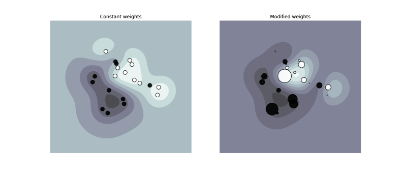
Figure 1: Effect of modifying weights on the decision function. Here, the size of points is proportional to its weight.

In the case of the traditional CS approach, the assigned cost value is applied to all the minority class instances indiscriminately and this raises a major concern [10]. All minority class instances do not pose the same level of difficulty. Samples that are closer to the decision boundary have a higher chance of getting misclassified than those that are far away. The more difficult-to-learn samples should be penalized more heavily than the others. This instance-level difficulty characteristic has not been considered in previous literature and our study addresses this issue. For instance, a dataset has an IR of 100. Then all the minority-class instances will be penalized 100 times more strongly than any majority-class instances. This will create some unusual deformation of the decision boundary and consequently, cause a higher number of misclassifications of the majority class instances (lower specificity score) during testing. Assigning unnecessarily high penalties to the minority-class samples that are located far away from the decision boundary only biases the predictions toward the minority-class and fails to generalize well on the test data. To mitigate the situation, an instance-difficulty-based cost should be applied. We propose such an algorithm termed ”iCost: Instance complexity-based Cost-sensitive learning” in this study.

Class overlapping is one of the major data difficulty factors that complicate the learning task when the data is imbalanced [4]. We try to address this issue in our proposed algorithm by first categorizing all the minority-class sample points based on their difficulty levels. We employ a neighborhood search algorithm to grade the samples into different levels. This is done based on the number of neighboring samples from the opposite class. A higher misclassification cost is assigned to the samples in the overlapping regions. This way, minority-class samples in the overlapped regions are prioritized significantly over the majority-class samples, leading to correct identifications of those hard-to-learn instances. On the other hand, samples that are in the safe zones surrounded by samples from the same class are marginally weighted, reducing their effect. The appropriate value for the penalty can be determined using grid search, evolutionary techniques, or similar approaches. This way, asymmetric cost is applied to different minority-class instances based on their complexity. This ensures a more appropriate distribution of weights among the minority-class instances. Thus, our proposed algorithm is able to provide improved prediction performance on a wide range of imbalanced datasets.

The proposed technique is implemented by inheriting classifiers from the sklearn library, ensuring full compatibility with Sklearn’s CS classifiers. Different ways of categorization of the minority-class instances are possible and some of them have been included in our implementation. The performance of the proposed approach is evaluated on 66 different imbalanced datasets. Significant improvements in performance have been observed as compared to other CS approaches as well as popular sampling techniques.

The rest of the article is organized as follows. Related works have been discussed in Section II. The proposed methodology is presented in Section III. In Section IV, we laid out the experimental setup. The performance measures are reported in Section V. The manuscript concludes with Section VI, with a summary of the work.

II Related Works

A lot of different techniques have been proposed over the years to deal with imbalanced data [2]. However, very few of them address data-intrinsic characteristics [11, 12]. Several data difficulty factors have been identified which include class overlapping, small disjunct, noisy samples, etc [13]. It has been suggested that the overlapping between the classes, not the imbalance, is primarily responsible for complicating the learning task [14]. Recent literature emphasizes the importance of considering data difficulty factors to develop more robust methods for learning from imbalanced datasets [13]. Stefanowski proposed several approaches to tackle these data difficulty factors [15]. However, the study only considers data resampling techniques. In this study, we are primarily focused on CS approaches.

Different classifiers such as SVM, ANN, and DTs are adapted to the CS framework [16, 17]. Their implementation is available in the popular sklearn library. In different medical datasets, class imbalance is prevalent and CS approaches are found to be quite successful in handling such scenarios [18]. Mohosheu et al. performed a detailed efficacy analysis of the performance of CS approaches as compared to data resampling techniques in their study [19]. The authors reported that the traditional CS approaches outperform undersampling and ensemble methods but cannot surpass popular oversampling techniques such as SMOTE or ADASYN. Hybridization between sampling and CS approaches is also possible and has been proposed by Newaz et al. [20]. The authors first resampled the data by generating synthetic samples using SMOTE and then used a weighted XGBoost classifier for training. The authors suggested that combining the techniques together allows for lower misclassification costs to be applied while also reducing the number of synthetic samples to be generated. Consequently, overfitting is reduced and better prediction performance can be obtained.

Gan et al. proposed a sample distribution probability-based CS framework in their article [21]. Roychoudhuri et al. adapted the CS algorithm for time-series classification [22]. Zhou et al. extended the CS framework for multiclass imbalanced scenarios [23]. Other variations of CS approaches include MetaCost [24], a meta-learning algorithm that converts any given classifier into a CS classifier. The idea of example-dependent cost has also been proposed in previous literature [25, 26]. For instance, in credit scoring, a borrower’s credit risk is determined based on different factors which include their credit history and financial behaviors. These factors should be taken into consideration while weighting instances for predictive modeling [27]. However, such approaches are application-specific and do not generalize well for other datasets. A detailed review of different CS methods has been presented in this recent article [28]. None of these CS approaches considers instance-difficulty-based characteristics. This has been pointed out in some recent literature [4, 10, 13] and we address this issue in our study.

III Methodology

In this section, we discuss our proposed algorithm in detail. At first, we identify the K-nearest neighbors of each minority class sample. A k-value of 5 was utilized in this study. The nearest neighbors are computed using the Euclidean distance. Next, each minority class instance is categorized as follows:

• Pure: Number of neighboring samples belonging to the majority class = 0

• Safe: Number of neighboring samples belonging to the majority class = 1 or 2

• Border: Number of neighboring samples belonging to the majority class $>2$

This has been illustrated in Fig. 2. Samples that are categorized as ’pure’ are completely surrounded by instances of the same class. These samples are easy to classify and are usually located far from the decision boundary. Hence, a comparatively much smaller misclassification cost should be enough to correctly identify these samples. Assigning a higher weight might worsen the scenario, resulting in a higher number of misclassifications of the majority class instances. ’Safe’ samples have 1 or 2 neighboring opposite-class instances. These samples should be handled carefully due to the risk of misclassification. Assigning too small a weight may be insufficient, while too large a weight could reverse the situation. On the other hand, border samples are surrounded by majority-class instances. These samples would be misclassified by the K-nearest neighbor classification rule. Therefore, a higher weight is necessary to prioritize these samples over the neighboring samples from the opposite class.

Figure 2: Categorization of Minority-class instances

In our implementation, different weights are assigned to different categories of samples based on their difficulty level. We employed a grid-search technique to determine the appropriate cost for different categories. The values varied from one dataset to another. Based on the experiments conducted on 66 datasets, we set a default value for each category for direct implementation. The default setting of the weights also provides quite an improvement in performance. The default penalty value for border samples is fixed as the IR of the dataset. For the safe samples, half of that value is utilized. For the ’pure’ category, a cost factor of 1.2 is selected which is almost the same as the misclassification cost of majority class samples. Employing different search algorithms to find the more suitable weights for individual datasets can optimize the prediction performance.

There are other ways of categorizing minority-class instances. One such way was proposed by Napierala et al. [29] where the samples are classified into four categories: safe, borderline, rare, and outliers. This is also implemented in our proposed framework by assigning four different penalties. Employing search algorithms to find a suitable set of four different values can be a bit more time-consuming. To give the user more freedom, we provide a general categorization formula based on the number of majority-class samples surrounding a minority-class instance. We grade each minority-class sample from g0 to g5 based on 0 to 5 neighboring majority-class samples, respectively. Then, different weights can be assigned to each type of minority-class sample based on its grade.

We implemented our proposed approach using the Python programming language. The theoretical framework behind cost-sensitive classifiers such as CS-SVM has been discussed in detail in previous literature [16] and therefore, not repeated in this manuscript. The implementation code can be found in the following repository: (the GitHub repo could not be released during submission due to blind review policy).

The architecture of our proposed algorithm is presented below:

Algorithm: Instance complexity-based Cost-sensitive learning (iCost)

Inputs:

• data: Input dataset (Pandas DataFrame)

• classifier: ’SVM’, ’LR’, or ’DT’ (default = ’SVM’). The algorithm inherits from Sklearn’s SVC, LogisticRegression, and DecisionTreeClassifier implementations, respectively.

• type: ’org’, ’ins’, ’nap’, or ’gen’ (default = ’ins’). ’org’ refers to the original implementation of the CS classifier. ’ins’ refers to the instance categorization criteria we proposed. ’nap’ refers to the instance categorization criteria proposed by Napierala et al. [29]. ’gen’ provides the general categorization mentioned earlier.

• k: The number of neighbors to be considered for categorization of the minority-class instances (default = 5).

• cost-factor: The misclassification cost to be assigned. It can be an integer or a list/dictionary. This input parameter is related to the ’type’ parameter. For type = ’org’, the cost-factor value must be an integer. For other types, the cost-factor value can be both an integer and a list/dictionary. For all cases, the default value is set as the IR of the dataset.

Output: Instance-level weighted classifier fitted on the given input training data.

Procedure:

• If type = ’org’, the algorithm assigns a weight equal to the cost factor to all the minority-class instances without any other consideration. This is the original CS implementation of the algorithms. If the cost factor value is 1, the algorithm will work as a standard ED classifier.

• If type = ’ins’ or ’nap’, the algorithm categorizes the minority-class instances into three or four categories, respectively. For ’gen’, minority-class instances are categorized into k+1 categories.

• In the case of ’ins’, the user can provide an integer or an array/dictionary with three elements as the input values for the cost factor. If it is an integer, then a penalty equal to the integer is assigned to the ’border’ samples. For the ’safe’ samples, half of the integer value is assigned as the penalty factor. For the ’pure’ samples, misclassification cost = 1.2 is fixed. If the input is an array, values are directly assigned to border, safe, and pure samples, in that order. In the case of a dictionary, key-value pairs can be used to directly state the cost values for each pair.

• Same thing goes for type = ’nap’. If the input value for the cost factor is an integer, then the weights are assigned to the minority class samples in the following way: outlier = cost factor, rare = 0.75 * cost factor, border = 0.5 * cost factor, and safe = 0.25 * cost factor. The user can also directly assign weights using an array or dictionary with four elements.

• For ’gen’, the user can assign weights using an array of k+1 elements. In the case of integer input or default scenario (weight=IR), the weight is equally divided between the samples from 1 to IR proportionally based on their grade.

• The appropriate values for the misclassification cost are dependent on the dataset. A value equal to the IR of the dataset is set as default, similar to the implementation of the sklearn library. The above-mentioned approach of assigning costs to different categories of samples provides a decent improvement in performance. However, it can be further optimized using different search algorithms [30].

• Any misclassifications of the majority class samples are assigned a weight of 1. Therefore, assigning a weight lower than 1 to any minority class instance can result in poor sensitivity in imbalanced classification tasks. Since minority-class samples are usually more important to classify correctly, a conditional statement is kept to ensure that the minimum weight assigned to any minority-class instance should not be lower than 1.

Example:

• iCost(data, classifier = ’LR’, type = ’gen’, cost-factor = [2, 2, 2, 10, 10, 10])

• This will apply an instance complexity-based cost-sensitive Logistic Regression (LR) classifier on the given data. Here, g0, g1, and g2 graded minority-class samples (’pure’ and ’safe’ categories) are weighted by a factor of 2. The remaining samples (’border’ category) are weighted by a factor of 10.

IV Experiment

IV-A Datasets

The performance of the proposed algorithm has been evaluated on 66 imbalanced datasets with varying degrees of imbalance to ensure the generalizability of the proposed approach. The datasets are collected from KEEL and the UCI data repository [31]. All the datasets are publicly available and with no missing entries. A summary of the datasets is provided in Table II.

TABLE II: Summary of the datasets

Dataset Name	# Samples	# Features	Imbalance Ratio
glass1	213	10	1.8
wisconsin	683	10	1.86
pima	768	9	1.87
glass0	213	10	2.09
yeast1	1483	9	2.46
vehicle2	846	19	2.88
vehicle1	846	19	2.9
vehicle3	846	19	2.99
vehicle0	845	19	3.27
new-thyroid1	215	6	5.14
ecoli2	336	8	5.46
glass6	214	10	6.38
yeast3	1484	9	8.1
yeast	1484	9	8.1
ecoli3	336	8	8.6
page-blocks0	5472	11	8.79
ecoli-0-3-4_vs_5	200	8	9
yeast-2_vs_4	514	9	9.08
ecoli-0-6-7_vs_3-5	222	8	9.09
ecoli-0-2-3-4_vs_5	202	8	9.1
yeast-0-3-5-9_vs_7-8	506	9	9.12
glass-0-1-5_vs_2	172	10	9.12
yeast-0-2-5-7-9_vs_3-6-8	1004	9	9.14
yeast-0-2-5-6_vs_3-7-8-9	1004	9	9.14
ecoli-0-4-6_vs_5	203	7	9.15
ecoli-0-2-6-7_vs_3-5	224	8	9.18
glass-0-4_vs_5	92	10	9.22
ecoli-0-3-4-6_vs_5	205	8	9.25
ecoli-0-3-4-7_vs_5-6	257	8	9.28
vowel	988	14	9.98
ecoli-0-6-7_vs_5	220	7	10
glass-0-1-6_vs_2	192	10	10.29
ecoli-0-1-4-7_vs_2-3-5-6	336	8	10.59
glass-0-6_vs_5	108	10	11
glass-0-1-4-6_vs_2	205	10	11.06
glass2	214	10	11.59
ecoli-0-1-4-7_vs_5-6	332	7	12.28
cleveland-0_vs_4	177	14	12.62
shuttle-c0-vs-c4	1829	10	13.87
yeast-1_vs_7	459	8	14.3
glass4	214	10	15.46
ecoli4	336	8	15.8
page-blocks-1-3_vs_4	472	11	15.86
abalone	731	9	16.4
glass-0-1-6_vs_5	184	10	19.44
yeast-1-4-5-8_vs_7	693	9	22.1
yeast4	1484	9	28.1
yeast128	947	9	30.57
yeast5	1484	9	32.73
winequality-red-8_vs_6	656	12	35.44
ecoli_013vs26	281	8	39.14
abalone-17_vs_7-8-9-10	2338	9	39.31
yeast6	1483	9	41.37
winequality-white-3_vs_7	900	12	44
winequality-red-8_vs_6-7	855	12	46.5
kddcup-land_vs_portsweep	1060	39	49.48
abalone-19_vs_10-11-12-13	1622	9	49.69
winequality_white	1481	12	58.24
poker-8-9_vs_6	1484	11	58.36
winequality-red-3_vs_5	691	12	68.1
abalone_20	1916	8	72.69
kddcup-land_vs_satan	1609	39	79.45
poker-8-9_vs_5	2074	11	81.96
poker_86	1477	11	85.88
kddr_rookkit	2225	42	100.14

IV-B Experimental Setup

To ensure proper validation and avoid data leakage, the data was first split into training and testing folds. The algorithms are applied only to the training set and the performance is evaluated on the testing set. A repeated stratified K-fold cross-validation strategy (5 folds, 10 repeats) was adopted to ensure better generalization. The average of the results from all different testing folds is considered as the performance measure.

We experimented with 3 different classification algorithms in this study: LR, SVM, and Decision Tree (DT). The default parameters of the Sklearn library were utilized to implement these classifiers. In the case of the proposed iCost algorithm, only the ’cost-factor’ parameter was tuned using the grid-search technique. We used type=’org’ and ’ins’ to obtain results for the traditional CS classifiers and our proposed modified CS approach, respectively. The parameter setting for the grid-search implementation is provided in Table III. MCC score was utilized as the scoring criteria.

TABLE III: Parameter settings for the grid-search implementation of the proposed iCost algorithm

Parameter	Value	Cost-factor parameter setting
Type	org	0.8*IR, IR, 1.2*IR
Type	ins	’pure’ : [1, 0.2*IR]
		’safe’: [0.25*IR, 0.35*IR, 0.5*IR]
		’border’: [0.75*IR, 0.9*IR, IR, 1.1*IR, 1.25*IR]

IV-C Performance Metrics

Assessing the performance of different techniques on skewed data can be challenging [1]. Eight different performance metrics were computed for evaluation in this study: MCC, ROC-AUC, G-mean, F1-score, sensitivity, specificity, precision, and accuracy. ML algorithms often excel at predicting instances from the majority class but tend to perform poorly on the minority class. Consequently, traditional performance metrics like accuracy can be misleading because they do not account for the distribution of classes. For instance, if 95% of the data belongs to one class and 5% to another, a model that always predicts the majority class will have 95% accuracy but will be useless for predicting the minority class. Sensitivity and specificity are two class-specific metrics that manifest the performance accuracy of the minority and majority classes, respectively. They only show the performance of a particular class. As a result, it is difficult to apprehend the entire performance spectrum from these measures.

Composite metrics are more suitable for performance measurements on imbalanced data. The g-mean score exhibits a broader picture by providing the geometric mean of sensitivity and specificity. F1-score provides the harmonic mean between sensitivity and precision. The algorithm needs to attain a high sensitivity to have a better G-mean or F1-score. While these two metrics are quite popular and have their advantages, there are certain issues and limitations associated with them. They do not consider the actual number of misclassifications. To elaborate, a sensitivity score of 0.8, observed with only 100 minority-class samples in the dataset, implies that the model misclassified 20 instances from the minority class. On the other hand, a specificity score of 0.8 with 10,000 majority-class samples in the same data indicates that the model misclassified 2,000 instances. This is a huge difference in the number of misclassifications which is not apparent from class-specific metrics. An algorithm may improve the sensitivity score to 0.9 which indicates that only 10 minority class instances have been misclassified. However, improving sensitivity often comes at the cost of lowering the specificity score. If the specificity score is reduced to 0.7 by the algorithm, then the model is now making 3000 misclassifications on the majority class. For both cases, the overall g-mean score remains almost the same. However, the model is now misclassifying around 1000 more samples which is not captured by these metrics.

To be more vigilant regarding performance measurements, we consider other metrics such as MCC and ROC-AUC. MCC provides a robust performance measure as it considers the actual number of misclassifications for both classes. This comprehensive consideration provides a balanced measure of model performance. The MCC score is high only when the classifier performs well across all cases, making it one of the most robust measures of classification performance. However, as stated in several previous literature [32, 33], the performance of algorithms on imbalanced data cannot be sufficiently represented by a single metric. Therefore, we take into consideration four composite metrics to understand how the proposed approach fares compared to other techniques used in imbalanced learning.

IV-D Performance Comparison

We compared the performance of the proposed approach with the standard CS learning technique to evaluate the differences. The results have also been compared with popular sampling techniques used in imbalanced learning. These include oversampling approaches such as SMOTE, ADASYN, Borderline-SMOTE (BL-SMOTE), and Random oversampling (ROS); undersampling techniques such as Random undersampling (RUS), Edited nearest neighbor (ENN), and Neighborhood cleaning (NC); hybrid sampling technique SMOTE-Tomek. Details of the performance measures from these approaches have been reported in the following section. The imblearn library was utilized to implement these sampling techniques using default parameter settings.

V Results and Discussion

In this section, we present and discuss the results we have obtained during the experiment. We have measured the performance of 3 different classifiers on 66 imbalanced datasets using 8 different metrics. All these measures cannot be included here due to space constraints. They are provided in separate supplementary files. We mainly considered the MCC, ROC-AUC, G-mean, and F1-score for comparison.

V-A Performance from traditional approaches

Standard classification algorithms do not perform well on imbalanced datasets. The performance gets even worse with higher imbalances and class overlapping [34]. In many cases, the g-mean score was found to be 0 (sensitivity=0, specificity=100), indicating a clear bias towards the majority class. Cost-sensitive learning (CSL) provides a significant improvement in performance as can be observed from Fig 3. Fig. 3 shows the average G-mean scores obtained on 66 datasets. Among the classifiers, CS-SVM provided the highest G-mean score. DT is found to be less sensitive to CS approaches. Improvement in performance was the maximum in the LR classifier. The average results from other metrics are provided in Table IV, Table V, and Table VI.

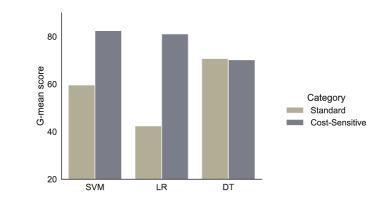
Figure 3: Performance comparison among standard and cost-sensitive approaches.

V-B Performance comparison of the proposed iCost algorithm with the standard CS approach

In this study, we propose a modification to the original implementation of CSL by introducing an instance complexity-based CS framework. In our approach, different misclassification costs are assigned to minority-class instances depending on their difficulty level. The samples located near the border are highly penalized compared to the samples that are away from the decision boundary or surrounded by instances of the same class. This ensures that the safe samples do not overshadow other majority-class instances and create unwarranted bias. Thus, our proposed approach provides a more plausible CSL framework where instances are weighted according to their complexity, rather than indiscriminately. This modification provides quite an improvement in performance.

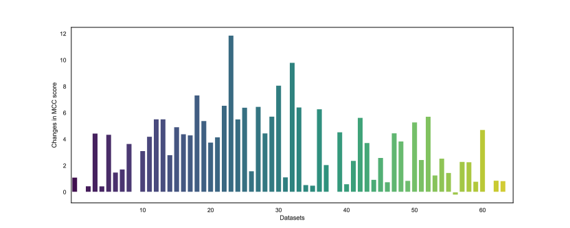
Figure 4: Changes in MCC score from the iCost algorithm as compared to traditional CS approach for the LR classifier on 66 datasets.

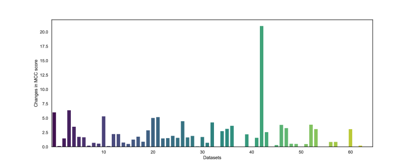
Figure 5: Changes in MCC score from the iCost algorithm as compared to traditional CS approach for the SVM classifier on 66 datasets.

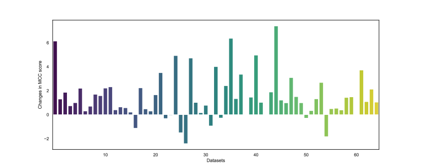
Figure 6: Change in MCC score from the iCost algorithm as compared to traditional CS approach for the DT classifier on 66 datasets.

The changes in the MCC score obtained from the proposed algorithm as compared to the traditional CS approach are presented in Fig. 4, Fig. 5, and Fig. 6 for the LR, SVM, and DT classifiers, respectively. As can be observed from Fig. 4, a significant improvement is noticeable in most datasets for the LR classifier. For a few datasets, there was no change in performance and for only one dataset, the performance dropped slightly. As for the SVM classifier, performance also improved in most datasets. However, the increment was lower than the LR classifier. In several of the datasets, the performance remained unchanged. This happened mostly in highly imbalanced cases (the datasets are sorted based on IR in ascending order). In such cases, the number of minority class samples is usually limited and they are surrounded by instances of the opposite class, leaving very few pure and safe samples. As a result, almost all the samples are border samples which are weighted equally and the algorithm works the same as the standard CS approach. In the case of the DT classifier, there was a deterioration in performance in some of the datasets. However, in most cases, it was almost negligible. As for the other datasets, there was a decent improvement in performance.

Overall, the most improvement was noticeable in the LR classifier (3.3% on average per dataset). For the other two classifiers, the improvement was around 2% on average. MCC is a highly reliable performance metric, and an improvement in MCC indicates that our proposed method effectively reduces the number of misclassifications. Fig. 7 demonstrates the other performance measures (average) obtained on 66 imbalanced datasets for the LR classifier. As can be observed from the figure, there is an increase in performance from the proposed algorithm over the traditional CS approach for almost all the measures. Only the sensitivity score dropped marginally. The number of minority class samples available in the datasets is usually very small. As a result, only a few misclassifications lead to a large change in the sensitivity score. However, in terms of all four composite metrics, the proposed algorithm achieved better results compared to the traditional CS approach. Similar improvements are noticeable for the SVM classifier as well (Table V.

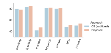
Figure 7: Average performance measures on 66 datasets for the LR classifier.

V-C Performance comparison of the proposed algorithm with other sampling techniques

We also compared the performance with some of the popular sampling approaches. Data resampling techniques undertake a completely different path in addressing the class imbalance and they have been widely applied in the imbalanced domain. The average of performance measures obtained from these approaches on the 66 imbalanced datasets are provided in Table IV, Table V, and Table VI for the LR, SVM, and DT classifiers, respectively.

As can be observed from the tables, the proposed framework produced better prediction performance compared to all the other approaches in terms of precision, ROC-AUC, G-mean, MCC, and F1-score. When the data was resampled using SMOTE, the most popular sampling technique, G-mean scores of 77.62% and 78.45% were obtained for the LR and SVM classifiers, respectively. Our proposed approach outperformed this well-established method by a large margin producing G-mean scores of 81.03% and 82.8%, respectively. A significant improvement in performance was noticeable compared to other approaches as well.

For both cases, the standard classifiers provided the highest specificity score due to the bias towards the majority class. For the SVM classifier, RUS provided the highest sensitivity score. However, RUS also attained the lowest specificity score. In RUS, a large number of majority-class samples are removed from the data to attain balance. Consequently, this approach provided the best performance for the minority class at the cost of the lowest performance for the majority class. This makes the prediction framework quite unreliable. A higher sensitivity score does not really indicate that the approach is actually performing well. MCC score manifests a more clear picture and the RUS approach produced a MCC score of 48.15%. Compared to that, the iCost algorithm achieved a much higher MCC score of 60.02%.

TABLE IV: Performance measures obtained from different approaches for the LR classifier

Metrics	LR	SMOTE	ADASYN	BL-SMOTE	ROS	RUS	ENN	NC	SMOTE_Tomek	CS-LR	iCost (Proposed)
Sensitivity	18.34	79.88	80.81	78.37	80.02	80.19	25.83	25.91	79.98	80.21	78.43
Specificity	99.16	80.46	78.16	80.77	79.70	75.16	96.40	96.30	80.44	83.26	85.47
Precision	33.64	46.70	42.75	45.56	45.46	41.65	36.05	37.31	46.69	41.87	47.13
ROC-AUC	58.75	80.17	79.48	79.57	79.86	77.67	61.11	61.10	80.21	81.73	81.95
G-mean	24.79	77.62	76.57	76.11	76.87	74.48	30.79	30.95	77.63	80.29	81.03
MCC	21.72	49.50	46.80	48.72	48.58	44.18	25.96	26.21	49.53	48.2	51.56
F1-score	21.81	52.47	49.94	51.90	51.53	47.50	27.83	28.10	52.46	50.57	53.96

TABLE V: Performance measures obtained from different approaches for the SVM classifier

Metrics	SVM	SMOTE	ADASYN	BL_SMOTE	ROS	RUS	ENN	NC	SMOTE_Tomek	CS-SVM	iCost(Proposed)
Sensitivity	41.21	77.28	78.64	74.10	77.19	83.37	51.32	51.64	77.30	78.12	76.53
Specificity	97.80	86.50	84.33	87.31	85.19	76.62	94.26	94.54	86.50	89.2	91.41
Precision	53.39	55.64	52.47	56.43	54.41	44.96	53.84	55.45	55.64	55.27	58.32
G-mean	48.47	78.45	78.03	76.05	77.70	76.43	54.78	55.25	78.46	81.05	82.8
MCC	42.99	56.13	54.05	55.59	54.80	48.15	47.24	48.23	56.14	57.99	60.02
ROC-AUC	69.51	81.89	81.49	80.70	81.19	79.99	72.79	73.09	81.90	83.66	83.97
F1-Score	43.98	58.07	56.26	57.95	57.03	50.57	49.03	49.86	58.07	60.03	61.97

TABLE VI: Performance measures obtained from different approaches for the DT classifier

Metrics	DT	SMOTE	ADASYN	BL_SMOTE	ROS	RUS	ENN	NC	SMOTE_Tomek	CS-DT	iCost(Proposed)
Sensitivity	55.46	62.18	63.38	60.07	53.73	81.81	61.39	62.48	62.20	54.69	56.1
Specificity	93.61	92.02	91.69	92.59	94.50	74.48	90.44	90.62	92.00	96	96.1
Precision	53.60	51.95	52.15	53.05	55.00	36.37	50.31	51.54	51.78	57.38	58.36
G-mean	65.34	70.53	70.80	68.46	63.22	76.29	68.58	68.71	70.47	65.14	69.91
MCC	48.32	50.04	50.49	49.83	48.29	41.07	48.24	49.57	49.92	51.39	52.73
ROC-AUC	74.54	77.10	77.53	76.33	74.12	78.14	75.92	76.55	77.10	75.05	76.1
F1-Score	51.87	53.45	53.71	53.21	51.19	44.09	52.16	53.12	53.34	54.68	55.9

VI Conclusion

In this study, a modified Cost-sensitive learning framework is proposed where data difficulty factors are taken into consideration while penalizing the instances. In the traditional framework, all the instances are weighted equally. This is impractical and can bias the prediction toward the minority-class, leading to an increased amount of false positives. Uniform instance weighting overfits the data by unusually deforming the decision boundary. This does not fare well during testing, resulting in a higher number of misclassifications. Class overlapping is identified as the most crucial difficulty factor that impairs prediction performance. To alleviate the issue, we weigh the minority-class samples in the overlapping region more strongly compared to the ones in the non-overlapping region. Carefully assigning higher weights to the hard-to-learn examples while reducing the weights of the other provides a more plausible weighting mechanism, resulting in fewer misclassifications. We have tested our algorithm on 66 imbalanced datasets using 3 different classifiers and observed an increment in performance in most cases. The proposed algorithm is computationally light similar to traditional CS approaches. The modification improves the CS framework by introducing some reasonable adjustments to it.

Only binary imbalanced classification scenarios have been considered in this study. The concept can be extended for multiclass scenarios as well. We plan to explore that in future works. While we worked with three different classifiers in this study, the proposed algorithm can be used with other classification algorithms such as Random Forest or XGBoost. The default values for the proposed approach are empirically set. Further research is required in this regard to understand how different data difficulty factors are related to the cost-factor values. We measured the instance complexity based on nearest neighbors. However, there are other data complexity measures such as local sets [35] which can also be considered. We plan to incorporate that into our framework in the future.

Supplementary files and codes are available in this repository: (could not be released during submission due to IEEE’s blind review policy).

References

- [1] P. Branco, L. Torgo, and R. P. Ribeiro, “A survey of predictive modeling on imbalanced domains,” ACM computing surveys (CSUR), vol. 49, no. 2, pp. 1–50, 2016.
- [2] G. Haixiang, L. Yijing, J. Shang, G. Mingyun, H. Yuanyue, and G. Bing, “Learning from class-imbalanced data: Review of methods and applications,” Expert systems with applications, vol. 73, pp. 220–239, 2017.
- [3] A. Fernández, S. García, M. Galar, R. C. Prati, B. Krawczyk, and F. Herrera, Learning from imbalanced data sets. Springer, 2018, vol. 10, no. 2018.
- [4] M. S. Santos, P. H. Abreu, N. Japkowicz, A. Fernández, and J. Santos, “A unifying view of class overlap and imbalance: Key concepts, multi-view panorama, and open avenues for research,” Information Fusion, vol. 89, pp. 228–253, 2023.
- [5] C. Elkan, “The foundations of cost-sensitive learning,” in International joint conference on artificial intelligence, vol. 17, no. 1. Lawrence Erlbaum Associates Ltd, 2001, pp. 973–978.
- [6] F. Shen, Y. Liu, R. Wang, and W. Zhou, “A dynamic financial distress forecast model with multiple forecast results under unbalanced data environment,” Knowledge-Based Systems, vol. 192, p. 105365, 2020.
- [7] W. Zhang, X. Li, X.-D. Jia, H. Ma, Z. Luo, and X. Li, “Machinery fault diagnosis with imbalanced data using deep generative adversarial networks,” Measurement, vol. 152, p. 107377, 2020.
- [8] A. Newaz, N. Ahmed, and F. S. Haq, “Diagnosis of liver disease using cost-sensitive support vector machine classifier,” in 2021 International Conference on Computational Performance Evaluation (ComPE). IEEE, 2021, pp. 421–425.
- [9] F. Pedregosa, G. Varoquaux, A. Gramfort, V. Michel, B. Thirion, O. Grisel, M. Blondel, P. Prettenhofer, R. Weiss, V. Dubourg, J. Vanderplas, A. Passos, D. Cournapeau, M. Brucher, M. Perrot, and E. Duchesnay, “Scikit-learn: Machine learning in Python,” Journal of Machine Learning Research, vol. 12, pp. 2825–2830, 2011.
- [10] A. Fernández, S. García, M. Galar, R. C. Prati, B. Krawczyk, F. Herrera, A. Fernández, S. García, M. Galar, R. C. Prati et al., “Cost-sensitive learning,” Learning from imbalanced data sets, pp. 63–78, 2018.
- [11] S. Rezvani and X. Wang, “A broad review on class imbalance learning techniques,” Applied Soft Computing, p. 110415, 2023.
- [12] B. Krawczyk, “Learning from imbalanced data: open challenges and future directions,” Progress in Artificial Intelligence, vol. 5, no. 4, pp. 221–232, 2016.
- [13] M. Dudjak and G. Martinović, “An empirical study of data intrinsic characteristics that make learning from imbalanced data difficult,” Expert systems with applications, vol. 182, p. 115297, 2021.
- [14] P. Vuttipittayamongkol, E. Elyan, and A. Petrovski, “On the class overlap problem in imbalanced data classification,” Knowledge-based systems, vol. 212, p. 106631, 2021.
- [15] J. Stefanowski, “Dealing with data difficulty factors while learning from imbalanced data,” in Challenges in computational statistics and data mining. Springer, 2015, pp. 333–363.
- [16] A. Iranmehr, H. Masnadi-Shirazi, and N. Vasconcelos, “Cost-sensitive support vector machines,” Neurocomputing, vol. 343, pp. 50–64, 2019.
- [17] Z.-H. Zhou and X.-Y. Liu, “Training cost-sensitive neural networks with methods addressing the class imbalance problem,” IEEE Transactions on knowledge and data engineering, vol. 18, no. 1, pp. 63–77, 2005.
- [18] I. D. Mienye and Y. Sun, “Performance analysis of cost-sensitive learning methods with application to imbalanced medical data,” Informatics in Medicine Unlocked, vol. 25, p. 100690, 2021.
- [19] M. S. Mohosheu, M. A. al Noman, A. Newaz, Al-Amin, and T. Jabid, “A comprehensive evaluation of sampling techniques in addressing class imbalance across diverse datasets,” in 2024 6th International Conference on Electrical Engineering and Information & Communication Technology (ICEEICT), 2024, pp. 1008–1013.
- [20] A. Newaz, M. S. Mohosheu, and M. A. Al Noman, “Predicting complications of myocardial infarction within several hours of hospitalization using data mining techniques,” Informatics in Medicine Unlocked, vol. 42, p. 101361, 2023.
- [21] D. Gan, J. Shen, B. An, M. Xu, and N. Liu, “Integrating tanbn with cost sensitive classification algorithm for imbalanced data in medical diagnosis,” Computers & Industrial Engineering, vol. 140, p. 106266, 2020.
- [22] S. Roychoudhury, M. Ghalwash, and Z. Obradovic, “Cost sensitive time-series classification,” in Machine Learning and Knowledge Discovery in Databases: European Conference, ECML PKDD 2017, Skopje, Macedonia, September 18–22, 2017, Proceedings, Part II 10. Springer, 2017, pp. 495–511.
- [23] Z.-H. Zhou and X.-Y. Liu, “On multi-class cost-sensitive learning,” Computational Intelligence, vol. 26, no. 3, pp. 232–257, 2010.
- [24] P. Domingos, “Metacost: A general method for making classifiers cost-sensitive,” in Proceedings of the fifth ACM SIGKDD international conference on Knowledge discovery and data mining, 1999, pp. 155–164.
- [25] Y. Zelenkov, “Example-dependent cost-sensitive adaptive boosting,” Expert Systems with Applications, vol. 135, pp. 71–82, 2019.
- [26] N. Günnemann and J. Pfeffer, “Cost matters: a new example-dependent cost-sensitive logistic regression model,” in Advances in Knowledge Discovery and Data Mining: 21st Pacific-Asia Conference, PAKDD 2017, Jeju, South Korea, May 23-26, 2017, Proceedings, Part I 21. Springer, 2017, pp. 210–222.
- [27] A. C. Bahnsen, D. Aouada, and B. Ottersten, “Example-dependent cost-sensitive logistic regression for credit scoring,” in 2014 13th International conference on machine learning and applications. IEEE, 2014, pp. 263–269.
- [28] G. Petrides and W. Verbeke, “Cost-sensitive ensemble learning: a unifying framework,” Data Mining and Knowledge Discovery, vol. 36, no. 1, pp. 1–28, 2022.
- [29] K. Napierala and J. Stefanowski, “Types of minority class examples and their influence on learning classifiers from imbalanced data,” Journal of Intelligent Information Systems, vol. 46, pp. 563–597, 2016.
- [30] L. Zhang and D. Zhang, “Evolutionary cost-sensitive extreme learning machine,” IEEE transactions on neural networks and learning systems, vol. 28, no. 12, pp. 3045–3060, 2016.
- [31] J. Derrac, S. Garcia, L. Sanchez, and F. Herrera, “Keel data-mining software tool: Data set repository, integration of algorithms and experimental analysis framework,” J. Mult. Valued Logic Soft Comput, vol. 17, pp. 255–287, 2015.
- [32] S. S. Mullick, S. Datta, S. G. Dhekane, and S. Das, “Appropriateness of performance indices for imbalanced data classification: An analysis,” Pattern Recognition, vol. 102, p. 107197, 2020.
- [33] A. Newaz, M. S. Mohosheu, M. A. Al Noman, and T. Jabid, “ibrf: Improved balanced random forest classifier,” in 2024 35th Conference of Open Innovations Association (FRUCT). IEEE, 2024, pp. 501–508.
- [34] M. S. Mohosheu, M. A. al Noman, A. Newaz, T. Jabid et al., “A comprehensive evaluation of sampling techniques in addressing class imbalance across diverse datasets,” in 2024 6th International Conference on Electrical Engineering and Information & Communication Technology (ICEEICT). IEEE, 2024, pp. 1008–1013.
- [35] M. S. Santos, P. H. Abreu, N. Japkowicz, A. Fernández, C. Soares, S. Wilk, and J. Santos, “On the joint-effect of class imbalance and overlap: a critical review,” Artificial Intelligence Review, vol. 55, no. 8, pp. 6207–6275, 2022.