The Asymptotic Behaviour of Information Leakage Metrics

Abstract

Information theoretic leakage metrics quantify the amount of information about a private random variable $X$ that is leaked through a correlated revealed variable $Y$. They can be used to evaluate the privacy of a system in which an adversary, from whom we want to keep $X$ private, is given access to $Y$. Global information theoretic leakage metrics quantify the overall amount of information leaked upon observing $Y$, whilst their pointwise counterparts define leakage as a function of the particular realisation $y$ that the adversary sees, and thus can be viewed as random variables. We consider an adversary who observes a large number of independent identically distributed realisations of $Y$. We formalise the essential asymptotic behaviour of an information theoretic leakage metric, considering in turn what this means for pointwise and global metrics. With the resulting requirements in mind, we take an axiomatic approach to defining a set of pointwise leakage metrics, as well as a set of global leakage metrics that are constructed from them. The global set encompasses many known measures including mutual information, Sibson mutual information, Arimoto mutual information, maximal leakage, min entropy leakage, $f$-divergence metrics, and g-leakage. We prove that both sets follow the desired asymptotic behaviour. Finally, we derive composition theorems which quantify the rate of privacy degradation as an adversary is given access to a large number of independent observations of $Y$. It is found that, for both pointwise and global metrics, privacy degrades exponentially with increasing observations for the adversary, at a rate governed by the minimum Chernoff information between distinct conditional channel distributions. This extends the work of Wu et al. (2024), who have previously found this to be true for certain known metrics, including some that fall into our more general set.

I Introduction

Consider a random variable $X$ which contains some sensitive information that should be kept private. Now let $Y$ be a correlated random variable, the value of which will be revealed to a potential adversary. The variables are connected via a noisy channel. To assess the privacy of the system, we must quantify the amount of information about $X$ that is contained in $Y$. There are countless ways in which this can be done, and, as a result, a great deal of privacy or ‘leakage’ metrics have been proposed and studied.

A subset of the measures proposed to evaluate privacy are information theoretic. We define an information theoretic leakage metric as one which quantifies the amount of information about $X$ that is leaked through $Y$. These must be upper bounded by some measure of the information held in $X$, which should depend on the distribution of $X$ only. A simple example of such a metric is the mutual information between $X$ and $Y$, which cannot be larger than the entropy of $X$. Conversely, differential privacy, a metric proposed by Dwork [1], which has since been extensively studied and even implemented by companies like Apple [2], is not an information theoretic leakage measure. It is a ratio of probabilities that can be arbitrarily large given the distribution of $X$. In this work, we consider information theoretic leakage measures.

Of the proposed privacy metrics, the vast majority are global measures [6, 7, 8, 4, 5]. By global, we mean that these measures take the joint distribution of $X$ and $Y$ and return a single number which quantifies the overall privacy of the system. Generally speaking, the information that the adversary learns about $X$ depends on which realisation $y$ they observe. There may be ‘good’ and ‘bad’ $y$’s which reveal little and much about $X$ respectively. It can be beneficial to see this represented in a privacy metric. The solution to this is to view leakage as a random variable. Privacy can be defined in a pointwise fashion, given an observation $Y=y$. As $Y$ is a random variable of which leakage is a function, we obtain a random leakage variable. Rather than a single number, the output contains the full spectrum of possible leakage values along with their probabilities. Saeidian, in [9], proposed this approach of viewing leakage as a random variable, and presented pointwise maximal leakage as a possible metric. She explains that this view allows us to make privacy guarantees based on the statistical properties of the leakage distribution, thus allowing for more flexibility than a global measure.

There are myriad ways in which to define privacy; in 2018, [6] reviewed over 80 proposed metrics. The important point to emphasise is that no single measure can be optimal for all applications. Suppose we have an adversary who will use $Y$ to guess a password $X$. Consider as a privacy metric the multiplicative increase in their probability of success upon observing $Y$. This metric will look different depending on how many password attempts the adversary is granted. As one can conceive of countless such application examples, we cannot hope to generate a finite list of all reasonable privacy metrics. This motivates an axiomatic view of privacy measures, which is an approach taken by [7] in the context of global measures. To the best of our knowledge, such a study on pointwise measures is yet to be done. We make progress on this topic in this paper.

Successive queries can undermine privacy mechanisms, and attacks are often sequential in nature [10]. An adversary with access to multiple observations of $Y$ may be able to infer more about $X$ than was allowed by design. As an illustration, suppose a data collector has a database containing useful but potentially sensitive health data about a number of individuals. They allow queries to be made on the data by organisations or individuals for research purposes, to which a perturbed response will be provided. An example of a query could be “How many of the individuals are over 65?”. The data collector may, for example, add noise to the true answer. Privacy can be degraded if multiple queries are allowed and responses are combined to reduce uncertainty. It is therefore of interest to analyse the behaviour of a leakage metric as a result of a number of observations, or in other words, derive composition theorems. Such results have previously been found for differential privacy [11] and for several global information theoretic measures [10]. In this work we study composition theorems for pointwise leakage metrics and for a general class of global leakage metrics.

Our main contributions are as follows.

1. We postulate the asymptotic behaviour of a reasonable information leakage metric under the composition of many observations. We consider what this should mean for global and pointwise measures respectively.

2. Taking an axiomatic view to defining a pointwise information theoretic privacy measure, we outline a set of axioms from which we will prove the desired asymptotic behaviour follows. More generally, the axioms serve as a list of properties that constitute a reasonable pointwise information theoretic privacy measure.

3. Following our definition of an information theoretic pointwise leakage metric, we define a corresponding set of global metrics. The set includes existing measures such as mutual information, Sibson mutual information, Arimoto mutual information, maximal leakage, min entropy leakage, $f$-divergence metrics, and g-leakage. It retains a great deal of flexibility to include new metrics that may be defined in the future. We prove that all metrics in the set satisfy the desired asymptotic conditions.

4. We prove that privacy defined according to our pointwise and global definitions degrades exponentially under the composition of many independent observations for the adversary, at a rate governed by the minimum Chernoff information between distinct conditional channel distributions. This was found to be true of a number of global metrics individually in [10].

We also draw parallels with the Bayesian approach to hypothesis testing, whereby the probability of error decays exponentially with the Chernoff information between the distribution of each hypothesis. The adversary’s estimate of $X$ can be viewed as a series of hypothesis tests, for which analytic properties are well established.

I-A Notation

Throughout the paper, random variables will be represented by capital letters and their realisations by lowercase letters. We denote private variables as $X$ and correlated observed variables as $Y$ with arbitrary but finite alphabets $\mathcal{X}$ and $\mathcal{Y}$ respectively. A series of $n$ observed random variables is given by $Y^{n}\in\mathcal{Y}^{n}$ where $\mathcal{Y}^{n}=\mathcal{Y}\times\dots\times\mathcal{Y}$. We use $\mathcal{P}_{\mathcal{X}}$ and $\mathcal{P}$ to represent the set of probability vectors over $\mathcal{X}$ and $\mathcal{Y}$ respectively, where the subscript $\mathcal{Y}$ is omitted from the latter for brevity as $\mathcal{P}$ appears frequently in proofs. Defined over $\mathcal{X}$, $E_{i}$ is a probability vector with $1$ in its $i$th position. This is equivalent to $E_{x}$ if $x=x_{i}$. We use $Q$ with a subscript to represent a true distribution. For example, the joint distribution of $X$ and $Y$ is $Q_{X,Y}$ and the conditional distribution of $Y$ given a realisation $X=x$ is $Q_{Y|X=x}$.

II Asymptotic Behaviour of Information Leakage

An information leakage metric quantifies the amount of information about a private variable $X$ that an adversary learns through an observed variable $Y$. An adversary cannot learn more than the maximum information contained in the private variable, and as a result information leakage must be upper bounded by a function of the distribution of $X$. We can use these metrics to assess the information leaked about the private variable through a series of observed variables. Let $X\sim Q_{X}$ and $Y\sim Q_{Y}$ where $X\in\mathcal{X}$ and $Y\in\mathcal{Y}$, for finite sets $\mathcal{X}$ and $\mathcal{Y}$. Suppose that the channel distribution $Q_{Y|X}$ is known, from which $n$ random samples $Y_{1},Y_{2},\dots,Y_{n}$ are drawn independent and identically distributed (i.i.d.) according to $Q_{Y|X=x}$. Therefore,

$$Q_{Y^{n}|X=x}(y_{1},\dots y_{n})=\prod_{i=1}^{n}Q_{Y|X=x}(y_{i}),$$ (1)

where $(y_{1},\dots y_{n})$ is a realisation of $Y^{n}$. Assume that the adversary observes $Y^{n}$. The asymptotic behaviour of an information leakage metric refers to its behaviour as $n$ grows large.

An essential property of an information leakage measure is that asymptotically, leakage should not decrease. As $n$ grows large, the adversary becomes more certain of the value of $X$. Asymptotically (i.e., in the limit of large $n$), upon receiving $n$ i.i.d. observations distributed according to $Q_{Y|X=x}$, an adversary knows $X=x$ with as much certainty as is possible through $Y$. This must not be any less than the certainty with which an adversary knows $X$ with fewer observations. Asymptotically, the information that the adversary learns about $X$ should thus be non-decreasing with $n$. We first discuss what this means for a global measure, before treating the pointwise case.

Global leakage concerns a private random variable $X$ and a correlated random variable $Y$ whose particular realisation is not specified. Global information leakage measures, commonly denoted by $\mathcal{L}(X\to Y)$ generate a single number that quantifies the amount of information about $X$ that is learned through observation of $Y$. They are real-valued functions defined over the set of all joint distributions of $X$ and $Y$ with finite but arbitrary alphabets. Let the global leakage for $n$ i.i.d. realisations of $Y$ be denoted by $\mathcal{L}_{n}\vcentcolon=\mathcal{L}(X\to Y^{n})$. It must be that $\mathcal{L}_{n}=g(Q_{X,Y^{n}})$ for some real-valued function $g$. For a fixed joint distribution $Q_{X,Y}$, we require that for integers $n\geq 1$,

$$\mathcal{L}_{n}\leq\mathcal{L}_{\infty}$$ (2)

and

$$\mathcal{L}_{n}\to\mathcal{L}_{\infty}$$ (3)

as $n\to\infty$, where $\mathcal{L}_{\infty}$ is a function of $Q_{X}$ only, and quantifies the amount of information in $X$. This says that as $n$ grows large, the global leakage about $X$ through $Y^{n}$ approaches the information in $X$ from below. On top of these asymptotic requirements, we argue that a global leakage measure should satisfy three axioms set out by Issa et al. [7, p. 1626]. These are as follows. Firstly, if $X$ and $Y$ are independent, the leakage through $Y$ about $X$ is zero. We call this the independence axiom. Secondly, if $X-Y-Z$ is a Markov chain, the global leakage from $X$ to $Z$ cannot be greater than that from $X$ to $Y$. This is the data processing axiom. Finally, if $(X_{1},Y_{1})$ is independent from $(X_{2},Y_{2})$, then $\mathcal{L}(X_{1},X_{2}\to Y_{1},Y_{2})=\mathcal{L}(X_{1}\to Y_{1})+\mathcal{L}(X_{2}\to Y_{2})$. We call this the additive axiom. As $X-Y^{n+1}-Y^{n}$ is a Markov chain, it follows from the data processing axiom that a global leakage measure should be monotonic in the sense that $\mathcal{L}_{n}\leq\mathcal{L}_{n+1}$. This says that, overall, leakage cannot decrease by giving the adversary more information.

Pointwise leakage is defined conditioned on a certain realisation, $Y=y$. The expression $\ell(X\to y)$ quantifies the leakage about $X$ to an adversary who observes $Y=y$. It is a function of the joint distribution over $X$ and $Y$ and the particular realisation $Y=y$. As $Y$ is a random variable, the pointwise leakage can be treated as one also. Let $l(y)\vcentcolon=\ell(X\to y)$. We say that $L\vcentcolon=l(Y)$ is the corresponding random leakage variable. Analogously to above, we use $L_{n}\vcentcolon=l(Y^{n})$ to denote the random amount of information leaked to an adversary who observes $n$ i.i.d. realisations of $Y$. In the pointwise case, the asymptotic statement is as follows. With probability one, there exists some $n^{\prime}\geq 1$ (which depends on the source realisation) such that for all $n\geq n^{\prime}$

$$L_{n}\leq L_{\infty}$$ (4)

and

$$L_{n}\to L_{\infty}$$ (5)

as $n\to\infty$ where $L_{\infty}$ is a random variable that is a function of $X$. This does not appear as strict as the global statement, the reason being simply that pointwise leakage depends on the realisation received. For finite $n$, it is possible that learning $y^{n}$ induces a larger leakage than learning the true value $x$. To understand this, note that some realisations of $X$ may contain more information than others. For instance, it is natural to intuit that more information is gained upon learning $X=x$ if $x$ was initially thought to be very unlikely, than if it was already expected. Consider the following example, where the true realisation of $X$ is $x_{2}$. Upon receiving $y^{n}$, an adversary had evidence favouring $X=x_{1}$ with some probability. They then learn with certainty that $X=x_{2}$. If the realisation $x_{1}$ contains more information than $x_{2}$, it is possible that the leakage was higher in the first instance than the second despite the adversary not being certain of $X$. As we would like to keep pointwise measures as general as possible, we allow those which may add more weight to knowledge gained about realisations that contain more information. In any case, as $n$ grows, the belief upon receiving $y^{n}$ gets closer to that having observed the true $x$. Eventually, the probability that $X=x_{1}$ becomes insignificant. At this point, $L_{n}$ must be smaller than $L_{\infty}$ as the adversary believes $X=x_{2}$ with high probability, but they are not certain. Intuitively we should see a convergence to $L_{\infty}$.

For pointwise measures, we cannot make the statement equivalent to $\mathcal{L}_{n}\leq\mathcal{L}_{n+1}$. To see this more clearly, we illustrate with an example. Suppose a survey is taken by a set of participants, half of which have a criminal record. The survey asks the question “Do you have a criminal record?”. So as to preserve plausible deniability, a sanitised version of survey answers is released in which the response to this question is switched with probability $1/6$. The scenario is depicted in Figure 1.

Figure 1: Joint distribution for criminal record survey response and sanitised output

Consider a single participant with no criminal record, and two adversaries. Adversary A is able to access two independent outcomes of the participant’s sanitised responses, whilst adversary B can only see the first. In other words, adversary A sees ($y_{1},y_{2}$) and adversary B sees $y_{1}$. Suppose $(y_{1},y_{2})=$(No,Yes). Adversary B now believes that the participant has no criminal record, with a probability of $5/6$ of her guess being correct. She has learned something about $X$, and intuitively a reasonable pointwise privacy metric will say that the leakage to adversary B is positive. On the other hand, adversary A’s belief over $X$ is unchanged. As was the case before making any observations, adversary A cannot favour either realisation of $X$ over the other. It is intuitive to say that he has not learned anything about $X$, and thus that the pointwise leakage should be zero.

II-A Global Leakage Example: Mutual Information

One of the most common and well understood measures of information leakage is mutual information. Mutual information is given by

$$I(X;Y)\vcentcolon=\sum_{x\in\mathcal{X}}\sum_{y\in\mathcal{Y}}Q_{X,Y}(x,y)\log\frac{Q_{X,Y}(x,y)}{Q_{X}(x)Q_{Y}(y)}.$$ (6)

This is a global information theoretic leakage measure; it takes as input the joint distribution over $X$ and $Y$ and outputs a single number which quantifies the amount of information about $X$ that is learned through $Y$, and it is upper bounded by a quantification of the information contained in $X$. We can say that $\mathcal{L}(X\to Y)=I(X;Y)$. It is established that mutual information satisfies the desired asymptotic properties (2-3), as well as monotonicity. We know that $I(X;Y^{n})\leq H(X)$. Wu et al. [10, Th. 1] proved that $\mathcal{L}_{n}\to\mathcal{L}_{\infty}$ as $n\to\infty$, where $\mathcal{L}_{\infty}=H(X)$ when the conditional probabilities $Q_{Y|X=x}$ are distinct. Moreover, the convergence occurs at a rate governed by the minimum Chernoff information between distinct conditional distributions $Q_{Y|X=x}$. It is well known that mutual information satisfies the data processing inequality, from which $\mathcal{L}_{n}\leq\mathcal{L}_{n+1}$ follows.

With the help of [10], the same properties can be verified of several other well established global leakage metrics. In this work, we will prove that they are satisfied for a generalised set of global information theoretic metrics.

II-B Pointwise Leakage Example: Pointwise Maximal Leakage

Work on pointwise leakage is far more scarce than that on global leakage in privacy literature. In particular, work regarding the asymptotic properties (4-5) does not exist to the best of our knowledge. Here, we take pointwise maximal leakage (PML) as our example measure. It will be proven in the following section that any pointwise leakage measure defined according to a set of axioms (of which PML is an example) satisfies our required asymptotic properties. In this section we use a numerical example to gain an intuition for how PML behaves under the composition of many i.i.d. observations.

PML was introduced as a privacy measure by Saeidian [9] in 2023, who defined and motivated the metric operationally. The paper also more generally argues the benefits of pointwise measures. Their operational definition is as follows. Let $U$ be some randomised function of $X$. The quantity $\ell_{U}(X\to y)$ is the logarithm of the ratio of the probability of correctly guessing $U$ having observed $y$, to the probability of correctly guessing $U$ with no observations. Pointwise maximal leakage is the supremum of $\ell_{U}(X\to y)$ over all distributions $Q_{U|X}$. Saeidian finds that this operational definition is equivalent to the following. With PML as the leakage metric, the amount of leakage of $X$ through a given observation $y$ is

$$l(y)=\log\max_{x:Q_{X}(x)>0}\frac{Q_{X|Y=y}(x)}{Q_{X}(x)},$$ (7)

and the associated random leakage variable is $L\vcentcolon=l(Y)$. If an adversary is allowed $n$ i.i.d. observations, the leakage becomes

$$l(y^{n})=\log\max_{x:Q_{X}(x)>0}\frac{Q_{X|Y^{n}=y^{n}}(x)}{Q_{X}(x)}.$$ (8)

Consider the discrete distribution $Q_{X,Y}$ in Figure 2.

Figure 2: Joint distribution for PML simulation with $(p,q,r)=(0.6,0.3,0.1)$, $s=0.4$

Through simulation, the empirical cumulative distribution functions (CDFs) of the random leakage shown in Figure 3 are produced.

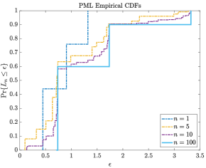
Figure 3: Empirical CDFs of PML as $n$ increases for the joint distribution specified in Fig. 2

By $n=100$, $L_{n}$ appears visibly to have converged to

$$L_{\infty}=\log\frac{1}{Q_{X}(X)}.$$ (9)

Three leakage values are possible, each corresponding to a realisation of $x$. The leakage corresponding to $X=x_{i}$ is $\log\frac{1}{Q_{X}(x_{i})}$. We can also see that each leakage value occurs with probability equal to the prior probability of the corresponding $x$. For smaller values of $n$, we see that generally the CDFs approach this limiting CDF as $n$ increases.

Consider the CDF of $L_{1}$. This leakage can also take three values, this time corresponding to each realisation of $y$. As $y_{1}$, $y_{2}$ and $y_{3}$ increase the posterior probability that $X$ is $x_{1}$, $x_{2}$ and $x_{3}$ respectively, $y_{1}$ induces the largest leakage value and $y_{3}$ the least. In fact, observing $Y=y_{1}$ or $Y=y_{2}$ induces a larger leakage than knowing for certain that $X=x_{1}$. Because the probability of observing $y_{3}$ is smaller than the prior probability of $x_{3}$, we see that the CDF of $L_{1}$ passes below the CDF of $L_{\infty}$ for some leakage values. This is an interesting property of pointwise leakage measures; values of $l$ and $n$ may exist such that $\Pr\{L_{n}\leq l\}<\Pr\{L_{\infty}\leq l\}$. Notice also that the minimum possible leakage is larger when $n=1$ than when $n=5$ or $n=10$. This is because conflicting observations, which can reduce the adversary’s certainty, are not possible in the case of a single query.

In the following section we will outline a set of axioms for a pointwise leakage measure from which we prove that our desired asymptotic properties follow. It can be verified that PML satisfies the axioms.

III Pointwise Leakage

In the previous section we presented a set of asymptotic properties that a reasonable pointwise information leakage measure should have. We have also gained an understanding of how one proposed pointwise leakage measure, PML, behaves under the composition of a large number of observations. The goal is now to prove that PML has the desired asymptotic properties, and further to identify what other reasonable pointwise leakage measures share them. To do this, we will take an axiomatic approach. We define a general pointwise leakage function. We further propose and motivate a set of axioms that dictate that the resulting measure is reasonable and natural. It can be verified that PML is in the set of allowed measures. Next, we will prove that all leakage metrics that follow the set of axioms share the desired asymptotic properties.

Recall that $X$ is a private random variable and $Y$ is a correlated public random variable with joint distribution $Q_{X,Y}$. We assume that the conditional distributions $Q_{Y|X=x}$, $x\in\mathcal{X}$ are all distinct (see Remark 1 for the case when this is not satisfied). A pointwise leakage measure $l(y)$ quantifies the resulting amount of leakage about $X$ upon learning $Y=y$. As $Q_{X}$ and $Q_{X|Y=y}$ represent the adversary’s knowledge about $X$ before and after receiving $Y=y$ respectively, it is reasonable to quantify leakage with a function of these two probability vectors. So, we consider a pointwise leakage function of the form

$$l(y)\vcentcolon=f(Q_{X|Y=y},Q_{X}),$$ (10)

for some real-valued function $f$ defined over $\mathcal{P}_{\mathcal{X}}\times\mathcal{P}_{\mathcal{X}}$, where $\mathcal{P}_{\mathcal{X}}$ is the set of probability vectors over $\mathcal{X}$. The first argument of the function is the posterior distribution (having observed $Y=y$) whilst the second is the prior. As $Y\sim Q_{Y}$ is a random variable, we further denote the pointwise leakage random variable $l(Y)$ by $L$.

Remark 1.

When the conditional distributions $Q_{Y|X=x}$, $x\in\mathcal{X}$ are not all distinct, we define a new random variable $\bar{X}$ which is obtained by grouping $x$ values that have the same conditional distributions. We can then define pointwise leakage as $f(Q_{\bar{X}|Y=y},Q_{\bar{X}})$, where $f$ is defined over $\mathcal{P}_{\bar{\mathcal{X}}}\times\mathcal{P}_{\bar{\mathcal{X}}}$. As the conditional distributions $Q_{Y|\bar{X}=\bar{x}}$ are distinct by construction, the analyses carried out in the paper remain valid for this case. Note that we can only compare the resulting leakage with the information in $\bar{X}$, rather than the information in $X$, which will never be learned in full.

This formulation retains enough flexibility for $f$ to be defined in a more complex way. For example, it is perfectly possible to define $f$ according to the operational definition of PML, which, as discussed in Section II-B, involves a maximisation over the distribution of a random variable $U$.

III-A Axioms of the Pointwise Leakage Function

In this section we define and motivate a set of properties that a pointwise leakage function should have. Let $P=(p_{1},p_{2},\dots,p_{|\mathcal{X}|})$, $Q=(q_{1},q_{2},\dots,q_{|\mathcal{X}|})$ be a pair of probability vectors over $|\mathcal{X}|$. A reasonable pointwise leakage function $f(P,Q)$ satisfies the following axioms for every $Q\in\mathcal{P}_{X}$.

1. $f(Q,Q)=0$.

2. For any $i\in\left\{1,\ldots,|\mathcal{X}|\right\}$, $f(E_{i},Q)>0$, where $E_{i}$ is a probability vector with $1$ as the $i$th element.

3. For any $k$ probability vectors $P_{1},P_{2},\dots,P_{k}$ and any coefficients $\lambda_{1},\lambda_{2},\dots,\lambda_{k}\geq 0$ such that $\sum_{i=1}^{k}\lambda_{i}=1$,

   $$f\left(\sum_{i=1}^{k}\lambda_{i}P_{i},Q\right)\leq\max_{i}f(P_{i},Q).$$

4. If $q_{i}\geq q_{j}$, then

   $$f(E_{i},Q)\leq f(E_{j},Q),$$

   where $E_{i}$ and $E_{j}$ are probability vectors with $1$ as the $i$th and $j$th element respectively.

5. For any $i\in\{1,2,\dots,|\mathcal{X}|\}$, $f(E_{i},Q)$ is a strict local maximum of the function $f(P,Q)$.

If the posterior distribution is identical to the prior, the adversary’s knowledge about $X$ is unchanged and the leakage must be zero. On the other hand, if the adversary learns the value of $X$ with certainty, leakage should be positive. This gives Axioms A1 and A2. We do allow $f(P,Q)$ to output negative values. Reasonable pointwise leakage metrics need not make use of this necessarily, but there are applications in which it can make operational sense. Consider a non-uniform distribution $Q_{X}$ and a channel $Q_{Y|X}$ such that $Q_{X|Y=y_{1}}$ is uniform. If the adversary observes $y_{1}$, their uncertainty about $X$ has increased. In certain applications (eg. password guessing) this may be strictly detrimental to the adversary and beneficial to the data owner. The loss in certainty may be reflected by a negative leakage value.

To understand A3, we can write

$$Q_{X|Y\in\{y_{1},\dots,y_{k}\}}=\sum_{i=1}^{k}\frac{Q_{Y=y_{i}}}{\sum_{j=1}^{k}Q_{Y=y_{j}}}Q_{X|Y=y_{i}}=\sum_{i=1}^{k}\lambda_{i}Q_{X|Y=y_{i}},$$ (11)

and so the condition becomes

$$f(Q_{X|Y\in\{y_{1},\dots,y_{k}\}},Q)\leq\max_{i}f(Q_{X|Y=y_{i}},Q).$$ (12)

The leakage to an adversary that knows that $Y\in\{y_{1},\dots,y_{k}\}$ cannot be any higher than the worst case.

We motivate A4 by noting that if the posterior distribution is $E_{i}$, the observer knows with certainty that $X=x_{i}$. The leakage therefore represents the information conveyed by the realisation that $X=x_{i}$, which should increase as the prior probability of $x_{i}$ decreases.

Finally, to see A5 we notice that, in a neighbourhood around $E_{i}$, moving closer to $E_{i}$ makes the observer more certain that $X=x_{i}$, which intuitively should increase the information leakage. The region in which this is true must exist but can be arbitrarily small. Consider Figure 4.

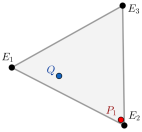
Figure 4: An example over the probability simplex $\mathcal{P}_{\mathcal{X}}$ with $|\mathcal{X}|=3$

Notice that the position of the prior, $Q$, means that the prior probability of $x_{3}$, $Q(x_{3})$, is small. Intuitively, the $x_{3}$ realisation contains a lot of information, and from many starting positions inside the simplex, moving towards $E_{3}$ should increase the information leakage. It is possible that $x_{3}$ dominates the behaviour of the leakage function throughout the majority of the simplex. Having said this, however small $Q(x_{3})$ is, it is possible to get close enough to $E_{1}$ or $E_{2}$ such that $P(x_{3})\ll Q(x_{3})$. At this point, we would not expect $x_{3}$ to dominate the pointwise leakage function. $P_{1}$ is an example of this. In conclusion, in a local region around $E_{i}$ (which may be arbitrarily small), moving $P$ towards $E_{i}$ should strictly increase the pointwise information leakage. This gives us A5.

There are some properties of the pointwise leakage function that are direct consequences of the axioms.

Corollary 1.

The global maximum of $f(P,Q)$ is $f(E_{i},Q)$, where $i=\arg\min_{i^{\prime}}q_{i^{\prime}}$.

Proof.

Any probability vector of length $|\mathcal{X}|$ can be expressed as $\sum_{i=1}^{|\mathcal{X}|}\lambda_{i}E_{i}$, where $\lambda_{1},\lambda_{2},\dots,\lambda_{|\mathcal{X}|}\geq 0$, $\sum_{i=1}^{|\mathcal{X}|}\lambda_{i}=1$. From A3 we know that

$$f\left(\sum_{i=1}^{|\mathcal{X}|}\lambda_{i}E_{i},Q\right)\leq\max_{i}f(E_{i},Q),$$

so the right hand side must be the global maximum. Employing A4 completes the proof. ∎

Corollary 1 is intuitive. The maximum possible leakage is achieved if we learn with certainty that $X=x_{i}$, where $x_{i}$ was the least likely $X$ realisation according to the prior distribution. Corollary 2 concerns the partial derivatives of $f$, and is important in later parts of the paper. We restrict our attention to continuous $f(P,Q)$, which can be smoothly extended to $\mathbb{R}^{|\mathcal{X}|}\times\mathbb{R}^{|\mathcal{X}|}$. Given any fixed $Q$, we also assume that $f(P,Q)$ is infinitely differentiable in a neighbourhood (in $\mathbb{R}^{|\mathcal{X}|}$) around all the extreme points $P=E_{x}$, $x\in\mathcal{X}$.

Let us now define what we call the derivative property.

Definition 1.

The function $f(P,Q)$ satisfies the derivative property if, for any $U\neq E_{i}$

$$(U-E_{i})\cdot\nabla f(P,Q)\big{|}_{P=E_{i}}<0,$$ (13)

i.e., the directional derivative in any feasible direction is negative when evaluated at an extreme point $P=E_{i}$.

This turns out often to be the case. Pointwise maximal leakage satisfies the derivative property. Also, we will see in Section IV-C (Table I) that this is the case of many existing global leakage metrics when expressed in a pointwise manner.

Corollary 2.

Let $f$ be a continuous function in both arguments. Also, assume that $f$ is differentiable at $(E_{i},Q)$ for all $i\in\{1,\ldots,|\mathcal{X}|\}$ and $Q\in\mathcal{P}_{\mathcal{X}}$. If $f$ satisfies the derivative property, then, for any $j\neq i$,

$$\frac{\partial f(P,Q)}{\partial p_{j}}\bigg{|}_{P=E_{i}}-\frac{\partial f(P,Q)}{\partial p_{i}}\bigg{|}_{P=E_{i}}<0.$$

Proof.

Consider the pair $(E_{i},Q)$ for an $i\in\{1,2,\ldots,|\mathcal{X}|\}$. By keeping $Q$ fixed, let us view $f$ as a function only in the first argument. As the function is differentiable at $E_{i}$, the gradient of $f$, $\nabla f$, is well defined and so are the directional derivatives. Due to the derivative property,

$$(U-E_{i})\cdot\nabla f(P,Q)\big{|}_{P=E_{i}}<0,$$

for all $U\neq E_{i}$. Rewriting this expression as a summation,

$$(U-E_{i})\cdot\nabla f(P,Q)\big{|}_{P=E_{i}} =\sum_{j=1}^{|\mathcal{X}|}(u_{j}-e_{ij})\frac{\partial f(P,Q)}{\partial p_{j}}\bigg{|}_{P=E_{i}}$$ (14)

$$=(u_{i}-1)\frac{\partial f(P,Q)}{\partial p_{i}}\bigg{|}_{P=E_{i}}+\sum_{j\neq i}u_{j}\frac{\partial f(P,Q)}{\partial p_{j}}\bigg{|}_{P=E_{i}}$$ (15)

$$=-\sum_{j\neq i}u_{j}\frac{\partial f(P,Q)}{\partial p_{i}}\bigg{|}_{P=E_{i}}+\sum_{j\neq i}u_{j}\frac{\partial f(P,Q)}{\partial p_{j}}\bigg{|}_{P=E_{i}}$$ (16)

$$=\sum_{j\neq i}u_{j}\left(\frac{\partial f(P,Q)}{\partial p_{j}}\bigg{|}_{P=E_{i}}-\frac{\partial f(P,Q)}{\partial p_{i}}\bigg{|}_{P=E_{i}}\right)<0,$$ (17)

where (16) follows from the fact that $U$ is a probability vector and thus $1-u_{i}=\sum_{j\neq i}u_{j}$. For (17) to be true for any $U\neq E_{i}$, Corollary 2 must hold. ∎

III-B Asymptotic Behavior of Pointwise Leakage and Composition Theorems

In this section we present the effects on pointwise leakage of the composition of many i.i.d. observations. Given the full system realisation $(x,y_{1},y_{2},\dots,y_{n})$, the pointwise leakage function is

$$l(y^{n})=f(Q_{X|Y^{n}=y^{n}},Q_{X}),$$ (18)

and the pointwise leakage random variable for $n$ i.i.d. observations is $L_{n}\vcentcolon=l(Y^{n}).$ Let $E_{x}$ be defined such that $E_{x}=E_{i}$, where $i$ is the index of $x$, i.e., $x_{i}=x$. We define an ‘information function’ which quantifies the amount of information contained in a particular realisation of $X$ as

$$i_{X}(x)\vcentcolon=f(E_{x},Q_{X}).$$ (19)

Like the pointwise leakage function, we may express this as a random variable. We define $I_{X}\vcentcolon=i_{X}(X)$ as the information random variable, and note that this is equal to $L_{\infty}$.

We introduce two theorems that characterise the asymptotic behaviour of the leakage random variable, $L_{n}$.

Theorem 1.

The sequence $L_{1},L_{2},\dots$ of pointwise leakage random variables converges almost surely to $I_{X}$ from below, i.e., with probability one,

$$L_{n}\to I_{X}$$

as $n\to\infty$, and there exists some $n^{\prime}\geq 1$ (which depends on the source realisation) such that for all $n\geq n^{\prime}$,

$$L_{n}\leq I_{X}.$$

This essentially says that if the adversary is allowed an arbitrarily large number of i.i.d. observations, they will learn all available information about $X$. Notice also that Theorem 1 aligns with the desired asymptotic properties for a pointwise information leakage measure outlined in Section II. Proof of Theorem 1 can be found in Section VII-C1.

Theorem 2 concerns the rate of convergence of $L_{n}$ to $I_{X}$. This is evaluated by comparing the CDFs. Let

$$F_{L_{n}}(l) \vcentcolon=\Pr\{L_{n}\leq l\},$$ (20)

$$F_{I_{X}}(l) \vcentcolon=\Pr\{I_{X}\leq l\}.$$ (21)

These will be referred to as the leakage CDF and information CDF, respectively. We will use the $L^{1}$-norm, $||F_{L_{n}}-F_{I_{X}}||_{1}$ to compare the CDFs. To motivate this, consider the following. Once the CDF of $L_{n}$ is identical to that of $I_{X}$, the adversary is learning all available information about $X$. Theorem 1 states that asymptotically, $L_{n}$ approaches $I_{X}$ from below, i.e., privacy does not improve with further observations. This means that, in the limit of large $n$, privacy worsens the closer the CDF of $L_{n}$ is to that of $I_{X}$. As the $L_{1}$ norm is a measure of the difference between two vectors, we can say that for large $n$ the rate of decay of the $L_{1}$ norm between the two CDFs is a natural way to quantify privacy degradation. Before stating Theorem 2, we must state that the Chernoff information between distributions $P_{1}$ and $P_{2}$ is defined as [12, p. 387]:

$$C(P_{1}||P_{2})\vcentcolon=-\min_{0\leq\lambda\leq 1}\log\left(\sum_{x}P_{1}^{\lambda}(x)P_{2}^{1-\lambda}(x)\right).$$ (22)

Note that base $2$ logarithms are used throughout.

Theorem 2.

The rate of decay of the $L^{1}$ norm between the pointwise leakage CDF and the information CDF is exponential and governed by the minimum Chernoff information.

$$\lim_{n\to\infty}\frac{1}{n}\log||F_{L_{n}}-F_{I_{X}}||_{1}\leq-\min_{x\neq x^{\prime}}C(Q_{Y|X=x}||Q_{Y|X=x^{\prime}}).$$ (23)

Equality is met if $f(P,Q)$ satisfies the derivative property.

The minimum Chernoff information has previously been found to govern the rate of convergence of certain global information theoretic privacy measures [10]. Theorem 2 extends these findings to any pointwise measure that satisfies the axioms given above. Proof of Theorem 2 can be found in Section VII-C2.

IV Global Leakage

A global information leakage metric takes as input the joint distribution $Q_{X,Y}$ and outputs a non-negative real number, which quantifies the overall privacy of the system. Here, we define a global leakage function in terms of a pointwise leakage function that is of the form given in (10). Given private data $X$, an adversary who observes $Y$, and a joint distribution $Q_{X,Y}$, the global leakage is

$$\mathcal{L}\vcentcolon=g_{2}\big{(}\mathbb{E}_{Y}\left[g_{1}\left(l(Y)\right)\right]\big{)},$$ (24)

where $g_{1}$ and $g_{2}$ are real-valued functions and $l(Y)$ is the pointwise leakage function of the form given in (10).

The idea behind $\mathbb{E}_{Y}[g_{1}(\cdot)]$ is that the user can combine the set of leakage values for realisations $y\in\mathcal{Y}$ in the way that best suits their application. For example, they should set $g_{1}$ as the identity function if they want a simple average to be taken over $Y$. The function $g_{2}$ is to suit the user’s preference. For example, many authors choose to take a logarithm so that they are working with units that are well understood. The combination of $f$, $g_{1}$ and $g_{2}$ should be chosen such that the result is a reasonable global information leakage measure. It should be upper bounded by some quantification of the information held in $X$. It should also be non-negative, and should satisfy the three axioms set out by [7, p. 1626]. These are the independence, data processing and additive axioms. Also, we would like the asymptotic requirements set out in Section II to be met. We address all properties in this section excluding the non-negative and additive properties, which should be verified independently when defining a global metric in the form of (24).

IV-A Constraints on the Global Leakage Function

Next, we outline certain properties that $g_{1}$ and $g_{2}$ should have so that the resulting global leakage metric is reasonable and natural. First, let the function $h$ be defined as the composition of $g_{1}$ and $f$, i.e.,

$$h(P,Q)\vcentcolon=g_{1}(f(P,Q)).$$ (25)

The contribution from realisation $y$ to the global leakage should increase with increasing pointwise leakage $l(y)$. Thus, $g_{1}$ should be strictly monotonic increasing. It is intuitive that the same is true of $g_{2}$. Note that this means $h$ must have the same local maxima as $f$. So that global leakage is zero when $X$ and $Y$ are independent, we require that $g_{1}$ and $g_{2}$ are defined such that $g_{2}(g_{1}(0))=0$. We will see that for many existing global leakage functions, $g_{2}=g_{1}^{-1}$. We also assert that $h(P,Q)$ must be convex in $P$. This ensures that the global leakage measure satisfies the data processing inequality, which is stated in Corollary 3.

Corollary 3.

If global leakage is defined according to (24), $h$ defined according to (25) is convex, and $X-Y-Z$ is a Markov chain where $X$ is the private variable,

$$\mathcal{L}(X\to Z)\leq\mathcal{L}(X\to Y),$$ (26)

i.e., the global leakage about $X$ through $Z$ is no greater than that through $Y$.

Proof.

The global leakage about $X$ from $Z$ is

$$g_{2}\left(\sum_{z\in\mathcal{Z}}Q_{Z}(z)h(Q_{X|Z=z},Q_{X})\right) =g_{2}\left(\sum_{z\in\mathcal{Z}}Q_{Z}(z)h\left(\sum_{y\in\mathcal{Y}}Q_{Y|Z}(y|z)Q_{X|Y=y},Q_{X}\right)\right)$$ (27)

$$\leq g_{2}\left(\sum_{z\in\mathcal{Z}}Q_{Z}(z)\sum_{y\in\mathcal{Y}}Q_{Y|Z}(y|z)h\left(Q_{X|Y=y},Q_{X}\right)\right)$$ (28)

$$=g_{2}\left(\sum_{y\in\mathcal{Y}}Q_{Y}(y)h(Q_{X|Y=y},Q_{X})\right),$$ (29)

where (27) uses the Markov chain and law of total probability, (28) applies the convexity of $h$, and (29) is the global leakage about $X$ from $Y$. ∎

Given an adversary who receives $n$ observations of $Y$ that are i.i.d. given $X$, the global leakage is

$$\mathcal{L}_{n}\vcentcolon=g_{2}\big{(}\mathbb{E}_{Y^{n}}\left[g_{1}\left(l(Y^{n})\right)\right]\big{)}=g_{2}\left(\sum_{y^{n}\in\mathcal{Y}^{n}}Q_{Y^{n}}(y^{n})g_{1}\left(f(Q_{X|Y^{n}=y^{n}},Q_{X})\right)\right).$$ (30)

As $X-Y^{n+1}-Y^{n}$ is a Markov chain, it immediately follows from Corollary 3 that $\mathcal{L}_{n}\leq\mathcal{L}_{n+1}$ and thus that $\mathcal{L}_{n}\leq\mathcal{L}_{\infty}$ for any finite $n$. As a further consequence of the properties of $h$, we can make a statement akin to Corollary 2 which will be used in later proofs.

Corollary 4.

For any $i$,

$$\frac{\partial h(P,Q)}{\partial p_{j}}\bigg{|}_{P=E_{i}}-\frac{\partial h(P,Q)}{\partial p_{i}}\bigg{|}_{P=E_{i}}<0$$

for all $j\neq i$.

Proof.

The proof follows from that of Corollary 2. As $h(P,Q)$ is convex in $P$ and its extreme points are local maxima, it must satisfy the derivative property. ∎

IV-B Composition Theorem for Global Leakage

The following theorem quantifies $\mathcal{L}_{\infty}$ and the rate at which $\mathcal{L}_{n}$ converges to $\mathcal{L}_{\infty}$.

Theorem 3.

Global leakage approaches its limit exponentially, at a rate equal to the minimum Chernoff information.

$$\lim_{n\to\infty}\frac{1}{n}\log\left(\mathcal{L}_{\infty}-\mathcal{L}_{n}\right)=-\min_{x\neq x^{\prime}}C(Q_{Y|X=x}||Q_{Y|X=x^{\prime}}),$$

where

$$\mathcal{L}_{\infty}\vcentcolon=g_{2}\left(\sum_{x\in\mathcal{X}}Q_{X}(x)g_{1}\left(f(E_{x},Q_{X})\right)\right).$$

Theorem 3 says that privacy, when defined according to (24), degrades at a rate governed by the minimum Chernoff information between distinct distributions $Q_{Y|X=x}$ and $Q_{Y|X=x^{\prime}}$. This result has been verified individually for mutual information, Sibson and Arimoto mutual information, and maximal leakage by [10]. The proof of Theorem 3 can be found in Section VII-D1.

IV-C Global Leakage Examples

We can express many existing global privacy measures in the form of (24). Table I illustrates this for mutual information, Sibson mutual information [13, 14, 15], Arimoto mutual information [14, 15], maximal leakage [7], $f$-divergence metrics [8], min entropy leakage and g-leakage [4, 5].

Table I: Existing global leakage metrics expressed in the form (24) and the corresponding pointwise leakage functions.

Leakage Metric	Standard Definition	$f(P,Q)$	$g_{1}(z)$	$g_{2}(z)$
Mutual information	$\sum\limits_{x,y}Q_{X,Y}(x,y)\log\frac{Q_{X,Y}(x,y)}{Q_{X}(x)Q_{Y}(y)}$	$D(P||Q)$	$z$	$z$
Sibson, $\alpha\in(1,\infty)$	$\frac{\alpha}{\alpha-1}\log\!\sum\limits_{y\in\mathcal{Y}}\left(\!\sum\limits_{x}Q_{X}(x)Q_{Y|X=x}(y)^{\alpha}\!\!\right)^{\!\frac{1}{\alpha}}$	$\log\left(\!\sum\limits_{i}q_{i}\left(\frac{p_{i}}{q_{i}}\right)^{\!\alpha}\!\right)$	$2^{\frac{z}{\alpha}}$	$\frac{\alpha}{\alpha-1}\log z$
Maximal leakage	$\log\sum\limits_{y}\max\limits_{x}Q_{Y|X=x}(y)$	$\log\max\limits_{i}\frac{p_{i}}{q_{i}}$	$2^{z}$	$\log{z}$
Arimoto, $\alpha\in(1,\infty)$	$\frac{\alpha}{\alpha-1}\log\sum\limits_{y}\left(\frac{\sum\limits_{x}Q_{X}(x)^{\alpha}Q_{Y|X=x}(y)^{\alpha}}{\sum\limits_{x}Q_{X}(x)^{\alpha}}\right)^{\frac{1}{\alpha}}$	$\log\frac{\sum_{i}p_{i}^{\alpha}}{\sum_{i}q_{i}^{\alpha}}$	$2^{\frac{z}{\alpha}}$	$\frac{\alpha}{\alpha-1}\log z$
$f$-divergence	$\sum\limits_{y}Q_{Y}(y)D_{\hat{f}}(Q_{X|Y=y}|Q_{X})$	$D_{\hat{f}}(P||Q)$	$z$	$z$
Min entropy leakage	$\log\sum\limits_{y}Q_{Y}(y)\frac{\max\limits_{x}Q_{X|Y=y}(x)}{\max\limits_{x}Q_{X}(x)}$	$\log\frac{\max\limits_{i}p_{i}}{\max\limits_{i}q_{i}}$	$2^{z}$	$\log z$
g-leakage	$\log\sum\limits_{y}Q_{Y}(y)\frac{\max\limits_{w\in\mathcal{W}}\sum\limits_{x}Q_{X|Y=y}(x)g(w,x)}{\max\limits_{w\in\mathcal{W}}Q_{X}(x)g(w,x)}$	$\log\frac{\max\limits_{w}\sum\limits_{i}p_{i}g_{i}(w)}{\max\limits_{w}\sum\limits_{i}q_{i}g_{i}(w)}$	$2^{z}$	$\log z$

Note that Sibson mutual information of order $1$ and $\infty$ correspond to mutual information and maximal leakage respectively. Arimoto mutual information of order $\alpha=1$ also gives standard mutual information. The $f$-divergence $D_{\hat{f}}(P||Q)$ is $\sum_{i}p_{i}\hat{f}\left(\frac{q_{i}}{p_{i}}\right)$. For a given global measure, the associated pointwise measure may not be unique. For example, mutual information could equally be represented by $f(P,Q)=\sum_{i}(p_{i}\log p_{i}-q_{i}\log q_{i})$, i.e., $f(Q_{X|Y=y},Q_{X})=H(X)-H(X|Y=y)$.

V Privacy and Hypothesis Testing

The composition results we have found are reminiscent of similar known results for Bayesian hypothesis testing. Indeed, we can use the latter to develop an intuition for these newer findings.

Consider a series of variables $Z_{1},Z_{2},\dots,Z_{n}$ that are distributed i.i.d. according to $P$. We wish to select one of two hypothesis: $H_{1}:P=P_{1}$ and $H_{2}:P=P_{2}$. We select $H_{1}$ if $z^{n}$ is in the acceptance region, $A_{n}\subseteq\mathcal{Z}^{n}$. If the hypothesis test is Bayesian, the error probability is [12, p. 395]

$$P_{e}^{(n)}=\pi_{1}P_{1}^{n}(A_{n}^{\mathrm{c}})+\pi_{2}P_{2}^{n}(A_{n}),$$ (31)

where $\pi_{1}$ and $\pi_{2}$ are prior probabilities for $H_{1}$ and $H_{2}$ respectively and $A_{n}^{\mathrm{c}}$ represents the complement of $A_{n}$. It turns out that to minimise the probability of error $A_{n}$ should be chosen according to a maximum a posteriori decision rule; if $i$ is the maximiser of $\pi_{i}P_{i}(z^{n})$, then $H_{i}$ is chosen. The probability of error decays exponentially with $n$ where the exponent is the Chernoff information between $P_{1}$ and $P_{2}$.

We now relate this to privacy by means of an example. Suppose $X\in\{x_{1},x_{2}\}$ is a binary private variable. An adversary accesses a series of random variables $Y_{1},Y_{2},\dots,Y_{n}$ that are i.i.d. given $X$. She conducts a Bayesian hypothesis test to determine $X$ where $H_{1}:P=Q_{Y|X=x_{1}}$ and $H_{2}:P=Q_{Y|X=x_{2}}$. Many privacy metrics compare the probability of an adversary making a correct guess before and after having made an observation. As an example, we will take min entropy leakage, a special case of g-leakage [4][5]. We can write

$$\mathcal{L}_{n}=\log\sum_{y^{n}\in\mathcal{Y}^{n}}Q_{Y^{n}}(y^{n})\frac{\max_{x\in\{x_{1},x_{2}\}}Q_{X|Y^{n}=y^{n}}(x)}{\max_{x\in\{x_{1},x_{2}\}}Q_{X}(x)},$$ (32)

which can be rearranged to give

$$\mathcal{L}_{n}=\log\frac{1-P_{e}^{(n)}}{1-P_{e}},$$ (33)

where $P_{e}$ is the adversary’s probability of an erroneous guess without any observations. Table I shows that min entropy leakage is in the set of global privacy metrics defined in Section IV. Thus by Theorem 3 we know that it approaches its limit, $\mathcal{L}_{\infty}$, exponentially at a rate governed by the Chernoff information. By Corollary 3, we know that this approach is from below and therefore that the asymptotic properties (2-3) are satisfied. This can equally be argued using the result from Bayesian hypothesis testing. We know that $1-P_{e}^{(n)}$ tends to $1$ from below exponentially according to the Chernoff information. The final result follows directly from the Taylor series expansion of the logarithm.

We can further intuit the case when $X$ is not binary. The adversary determines $X$ by pointwise comparison, testing all pairings $x,x^{\prime}$. The error probability that decays the slowest and is therefore the only relevant term in the limit of large $n$ is that of the pair with the smallest Chernoff information. The exponent is $\min_{x\neq x^{\prime}}C\left(Q_{Y^{n}|X=x},Q_{Y^{n}|X=x^{\prime}}\right)$, as we have found previously.

VI Discussion and Conclusions

We have discussed the essential asymptotic properties that an information leakage measure should satisfy. Namely, under the composition of a large number of observations for the adversary, leakage should approach its limit from below. We have outlined what this means for global and pointwise measures respectively, and used the arguments to motivate a set of axioms that a reasonable pointwise measure should follow. A set of corresponding global measures was defined which retains a great deal of generality and flexibility, and encompasses many existing measures. Thus, any pointwise or global privacy metrics proposed in future may well satisfy A1-A5 or fall within our global set respectively. The asymptotic properties of such metrics could straightforwardly be obtained from this paper. Future work may seek to generalise the global set further, in order to encompass all ‘reasonable’ global information leakage metrics, analogously to the pointwise result.

For the given pointwise and global metrics, we provided composition theorems which state that privacy degrades exponentially according to the minimum Chernoff information between distinct pairs $Q_{Y|X=x},Q_{Y|X=x^{\prime}}$. Defined as a random variable, pointwise leakage tends almost surely to the random information contained in the private variable $X$. It is worth noting that a pointwise measure need not be a reasonable information leakage metric according to A1-A5 to follow Theorem 2. Specifically, A1-A4 need not be followed. This is because of the underlying fact that as $n\to\infty$ the posterior distribution of $X$ converges almost surely to one of the extreme points of the simplex, $E_{i}$. So, when the function is sufficiently smooth at the extreme points, Theorem 2 may hold. Whilst we say that a reasonable pointwise information leakage metric should follow all five axioms for the reasons detailed in Section III-A, the subsequent analysis only requires A5. Thus, the result encompasses but is not restricted to so called ‘reasonable pointwise information leakage metrics’. Future work could explore further applications of Theorem 2, as well as the consequences of A1-A4 on the behaviour of a reasonable pointwise information leakage metric.

Finally, we discussed the connection between privacy and Bayesian hypothesis testing. The takeaway point is that the mathematics underpinning composition theorems for privacy metrics can be understood via the setting of Bayesian hypothesis testing. Underlying both is the method of types. This is because all of the measures are functions of $Q_{Y^{n}|X}$ where analysis of types naturally appears.

VII Proofs of the Main Results

VII-A Notation

To follow the proofs, some further notation is required (most of which follows that of [10]). Base $2$ logarithms are assumed. It will be important to note that probabilities of random variables are themselves random variables. For example, $Q_{Y|X=x}(Y)$ is a random variable representing the probability of observing $Y$, the random output of $Q_{Y|X=x}$.

The argument,

$$x^{\star}(y^{n})\vcentcolon=\arg\max_{x}Q_{Y^{n}|X=x}(y^{n}),$$ (34)

is the adversary’s maximum likelihood estimate (MLE) for $x$. Where appropriate $x^{\star}$ and $X^{\star}$ are written as $x^{\star}(y^{n})$ and $x^{\star}(Y^{n})$ respectively to emphasise their dependence on the adversary’s observations. The set $\mathcal{P}_{n}$ contains all possible empirical distributions corresponding to a length $n$ sequence over $\mathcal{Y}$; to each $y^{n}$, we can associate an empirical distribution $P_{n}\in\mathcal{P}_{n}$. Meanwhile, $\mathcal{P}$ is the set of all possible distributions over $\mathcal{Y}$, and any $P\in\mathcal{P}$ represents one of these possible distributions. Also let $T(P_{n})$ be the set of $y^{n}\in\mathcal{Y}^{n}$ whose empirical distribution is $P_{n}$. As it is frequently used, the distribution $Q_{Y|X=x}$ is shortened to $Q_{x}$. Next, let $x_{k}(P)$ represent the $x$ realisation that induces the $k$th smallest Kullback-Leibler divergence, $D(P||Q_{x})$, across all possible realisations $x\in\mathcal{X}$; i.e., $D(P||Q_{x_{1}(P)})=\min_{x}D(P||Q_{x})$. We also define $x$-domains as follows:

$$D_{x} \vcentcolon=\left\{P\in\mathcal{P}|D(P||Q_{x})<D(P||Q_{x^{\prime}})\;\forall x^{\prime}\in\mathcal{X}\right\},$$ (35)

For brevity, let

$$C_{n} \vcentcolon=\inf_{P_{n}\in\mathcal{P}_{n}}D(P_{n}||Q_{x_{2}(P_{n})}),$$ (36)

$$C \vcentcolon=\min_{x\neq x^{\prime}}C(Q_{x}||Q_{x^{\prime}}).$$ (37)

We call the latter the minimum Chernoff information.

VII-B Auxiliary Remarks and Lemmas

We can make three remarks which will frequently be pertinent throughout the proofs.

Remark 2.

If $P_{n}$ is the empirical distribution of $y^{n}$,

$$x_{1}(P_{n})=x^{\star}(y^{n}).$$ (38)

By noting that $P_{n}(y)$ is the fraction of occurrences of $y$ in $y^{n}$, it follows that

$$x^{\star}(y^{n}) =\arg\max_{x}Q_{Y^{n}|X=x}(y^{n})$$ (39)

$$=\arg\max_{x}\prod_{y\in\mathcal{Y}}Q_{Y|X=x}(y)^{nP_{n}(y)}$$ (40)

$$=\arg\max_{x}\sum_{y\in\mathcal{Y}}P_{n}(y)\log Q_{Y|X=x}(y)$$ (41)

$$=\arg\min_{x}\sum_{y\in\mathcal{Y}}P_{n}(y)\log\frac{P_{n}(y)}{Q_{Y|X=x}(y)}$$ (42)

$$=\arg\min_{x}D(P_{n}||Q_{x})=x_{1}(P_{n}).$$ (43)

We note that if there are multiple $x$ values with the same minimum $D(P_{n}||Q_{x})$, these $x$ values also all have the same maximum $Q_{Y^{n}|X=x}(y^{n})$. In this case we set by convention that $x_{1}(P_{n})=x^{\star}(y^{n})$.

Remark 3.

By standard continuity arguments [16, eq. 55],

$$\lim_{n\to\infty}\inf_{P_{n}\in\mathcal{P}_{n}}D(P_{n}||Q_{x_{2}(P_{n})})=\inf_{P\in\mathcal{P}}D(P||Q_{x_{2}(P)}),$$ (44)

as $D(P||Q_{x_{2}(P)})$ is a continuous function of $P$.

Remark 4.

It follows from Remark 3 and from the result of [10, Lemma 4] which is

$$\inf_{P\in\mathcal{P}}D(P||Q_{x_{2}(P)})=\min_{x\neq x^{\prime}}C(Q_{x}||Q_{x^{\prime}}),$$ (45)

that $\lim_{n\to\infty}C_{n}=C$. More precisely, there exists some positive integer $N$ such that for any $n\geq N$, $|C_{n}-C|\leq\frac{1}{\sqrt{n}}$.

Let us also define the set $\mathcal{\widetilde{P}}_{n}\subseteq\mathcal{P}_{n}$ as the set of $P_{n}\in\mathcal{P}_{n}$ satisfying

$$C_{n}-D(P_{n}||Q_{x_{1}(P_{n})})\geq\frac{1}{\sqrt{n}}.$$ (46)

We denote the corresponding set of possible $y^{n}$ sequences as $\widetilde{\mathcal{Y}}_{n}$. The set can be visualised on a probability simplex, as shown in Figure 5, where $\hat{P}_{n}$ is the argument of $C_{n}$.

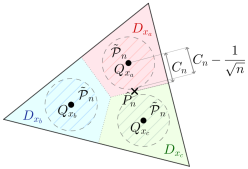
Figure 5: An example over the probability simplex $\mathcal{P}$ with $|\mathcal{Y}|=3$

We outline five lemmas in turn to prove Theorems 1 and 2. Lemma 1 says that when $n$ is large, $y^{n}$ lies within $\widetilde{\mathcal{Y}}_{n}$ with high probability, which will allow us to restrict the majority of our analysis to the set. Lemma 2 is the crux of the proof. It says that, with high probability, $Q_{X|Y^{n}=y^{n}}$ tends to $E_{x^{\star}}$ as $n$ grows large. Lemma 3 makes use of Lemma 2 to say that, for $y^{n}\in\widetilde{\mathcal{Y}}^{n}$, the pointwise leakage function approaches the information function of $x^{\star}(y^{n})$ from below with increasing $n$. In turn, Lemma 4 says that the distribution of $x^{\star}(Y^{n})$ approaches the distribution of $X$. Finally, Lemma 5 combines Lemmas 3 and 4 to bound the difference between the pointwise leakage CDF and the information CDF at any given point. Lemmas 1-4 are used along with the Borel-Cantelli Lemma to prove Theorem 1. Lemma 5 is used to prove Theorem 2. To prove Theorem 3, we introduce Lemma 6, which adapts Lemma 3 for use in the global setting.

Lemma 1.

For all large enough $n$, the probability of a sequence $y^{n}$ lying outside the set $\widetilde{\mathcal{Y}}_{n}$ decreases exponentially with $n$ at a rate governed by the minimum Chernoff information,

$$\sum_{y^{n}\not\in\widetilde{\mathcal{Y}}_{n}}Q_{Y^{n}}(y^{n})\leq\psi,$$ (47)

where

$$\psi\vcentcolon=|\mathcal{X}|(n+1)^{|\mathcal{Y}|}2^{-n\left(C-\frac{2}{\sqrt{n}}\right)}.$$ (48)

Proof.

$$\sum_{y^{n}\not\in\widetilde{\mathcal{Y}}_{n}}Q_{Y^{n}}(y^{n}) =\sum_{P_{n}\not\in\widetilde{\mathcal{P}}_{n}}\sum_{x\in\mathcal{X}}Q_{Y^{n}|X=x}(T(P_{n}))Q_{X}(x)$$ (49)

$$\leq\sum_{P_{n}\not\in\widetilde{\mathcal{P}}_{n}}\sum_{x\in\mathcal{X}}2^{-nD(P_{n}||Q_{x})}$$ (50)

$$\leq|\mathcal{X}|\sum_{P_{n}\not\in\widetilde{\mathcal{P}}_{n}}2^{-nD(P_{n}||Q_{x_{1}(P_{n})})}$$ (51)

$$\leq|\mathcal{X}|(n+1)^{|\mathcal{Y}|}2^{-n\left(C_{n}-\frac{1}{\sqrt{n}}\right)}$$ (52)

$$\leq|\mathcal{X}|(n+1)^{|\mathcal{Y}|}2^{-n\left(C-\frac{2}{\sqrt{n}}\right)}$$ (53)

where (50) follows from [12, Th. 11.1.4], (51) follows from the definition of $x_{1}(P)$, (52) follows from the definition of $\widetilde{\mathcal{P}}_{n}$ (46), and (53) follows from Remark 4. ∎

As $C$ is constant, we can conclude from Lemma 1 that

$$\lim_{n\to\infty}\sum_{y^{n}\not\in\widetilde{\mathcal{Y}}^{n}}Q_{Y^{n}}(y^{n})=0.$$ (54)

Lemma 2 is the crux of the proof and says that, with high probability, the posterior distribution $Q_{X|Y^{n}=y^{n}}$ approaches $E_{x^{\star}}$ as $n$ grows large.

Lemma 2.

For all $P_{n}\in\widetilde{\mathcal{P}}_{n}$ and $n$ large enough,

$$\left|Q_{X|Y^{n}=y^{n}}(x)-E_{x^{\star}}(x)\right|\leq\frac{1}{\min_{x}Q_{X}(x)}2^{-nK(P_{n})}$$ (55)

for any $x\in\mathcal{X}$, and

$$\frac{1}{2}\min_{x}Q_{X}(x)2^{-nK(P_{n})}\leq 1-Q_{X|Y^{n}=y^{n}}(x^{\star})\leq\frac{1}{\min_{x}Q_{X}(x)}2^{-nK(P_{n})},$$ (56)

where

$$K(P_{n})\vcentcolon=D(P_{n}||Q_{x_{2}(P_{n})})-D(P_{n}||Q_{x^{\star}}).$$ (57)

Proof.

First, consider the probability $Q_{X|Y^{n}=y^{n}}(x^{\star})$.

$$Q_{X|Y^{n}=y^{n}}(x^{\star}) =\frac{Q_{Y^{n}|X=x^{\star}}(y^{n})Q_{X}(x^{\star})}{Q_{Y^{n}}(y^{n})}$$ (58)

$$=\frac{2^{-nD(P_{n}||Q_{x^{\star}})}Q_{X}(x^{\star})}{2^{-nD(P_{n}||Q_{x^{\star}})}Q_{X}(x^{\star})+\sum_{x\neq x^{\star}}2^{-nD(P_{n}||Q_{x})}Q_{X}(x)}$$ (59)

$$=\left(1+\frac{2^{nD(P_{n}||Q_{x^{\star}})}}{Q_{X}(x^{\star})}\sum_{x\neq x^{\star}}Q_{X}(x)2^{-nD(P_{n}||Q_{x})}\right)^{-1}.$$ (60)

To establish a lower bound, we can bound the summation.

$$\sum\limits_{x\neq x^{\star}}Q_{X}(x)2^{-nD(P_{n}||Q_{x})} \leq\sum\limits_{x^{\prime}\neq x^{\star}}Q_{X}(x)\max\limits_{x\neq x^{\star}}2^{-nD(P_{n}||Q_{x})}$$ (61)

$$=\left(1-Q_{X}(x^{\star})\right)2^{-nD(P_{n}||Q_{x_{2}(P_{n})})}$$ (62)

$$\leq 2^{-nD(P_{n}||Q_{x_{2}(P_{n})})}.$$ (63)

Substituting this into (60) we find

$$Q_{X|Y^{n}=y^{n}}(x^{\star}) \geq\left(1+\frac{1}{Q_{X}(x^{\star})}2^{-nK(P_{n})}\right)^{-1}$$ (64)

$$\geq 1-\frac{1}{Q_{X}(x^{\star})}2^{-nK(P_{n})}$$ (65)

$$\geq 1-\frac{1}{\min_{x}Q_{X}(x)}2^{-nK(P_{n})}.$$ (66)

Looking now for an upper bound, we continue from (60).

$$Q_{X|Y^{n}=y^{n}}(x^{\star}) \leq\left(1+\frac{2^{nD(P_{n}||Q_{x^{\star}})}}{Q_{X}(x^{\star})}Q_{X}(x_{2}(P_{n}))2^{-nD(P_{n}||Q_{x_{2}(P_{n})})}\right)^{-1}$$ (67)

$$\leq 1-\frac{Q_{X}(x_{2}(P_{n}))}{Q_{X}(x^{\star})}2^{-nK(P_{n})}+\frac{Q_{X}(x_{2}(P_{n}))^{2}}{Q_{X}(x^{\star})^{2}}2^{-2nK(P_{n})}$$ (68)

$$\leq 1-\min_{x}Q_{X}(x)2^{-nK(P_{n})}+\frac{1}{\min_{x}Q_{X}(x)^{2}}2^{-2nK(P_{n})}.$$ (69)

As $P_{n}\in\widetilde{\mathcal{P}}_{n}$, $2^{-2nK(P_{n})}$ decays faster than $2^{-nK(P_{n})}$ and we can say that eventually,

$$\frac{1}{2}\min_{x}Q_{X}(x)2^{-nK(P_{n})}\geq\frac{1}{\min_{x}Q_{X}(x)^{2}}2^{-2nK(P_{n})}.$$ (70)

Thus, for $n$ large enough,

$$Q_{X|Y^{n}=y^{n}}(x^{\star})\leq 1-\frac{1}{2}\min_{x}Q_{X}(x)2^{-nK(P_{n})}.$$ (71)

Putting the results together we have bounds on $E_{x^{\star}}(x^{\star})-Q_{X|Y^{n}=y^{n}}(x^{\star})=1-Q_{X|Y^{n}=y^{n}}(x^{\star})$ as in (56). From this we can say that when $x\neq x^{\star}$

$$Q_{X|Y^{n}=y^{n}}(x)-E_{x^{\star}}(x)=Q_{X|Y^{n}=y^{n}}(x) \leq 1-Q_{X|Y^{n}=y^{n}}(x^{\star})$$ (72)

$$\leq\frac{1}{\min_{x}Q_{X}(x)}2^{-nK(P_{n})},$$ (73)

and therefore for any $x\in\mathcal{X}$, we have (55). ∎

We next make use of Lemma 2 to state Lemma 3.

Lemma 3.

For any observation $y^{n}$ whose type $P_{n}\in\widetilde{\mathcal{P}}^{n}$, the pointwise leakage function is bounded by the information function as follows for large enough $n$. For a general pointwise information leakage function

$$i_{X}(x^{\star}(y^{n}))-\theta_{0}2^{-nK(P_{n})}\leq l_{n}(y^{n})\leq i_{X}(x^{\star}(y^{n})),$$ (74)

and for a pointwise information function with the derivative property (13)

$$i_{X}(x^{\star}(y^{n}))-\theta_{1}2^{-nK(P_{n})}\leq l_{n}(y^{n})\leq i_{X}(x^{\star}(y^{n}))-\theta_{2}2^{-nK(P_{n})},$$ (75)

where

$$\theta_{0} \vcentcolon=\frac{\lambda|\mathcal{X}|}{\min_{x}Q_{X}(x)},$$ (76)

$$\theta_{1} \vcentcolon=\frac{3\beta}{2\min_{x}Q_{X}(x)},$$ (77)

$$\theta_{2} \vcentcolon=\frac{\gamma}{4}\min_{x}Q_{X}(x),$$ (78)

for some strictly positive constants $\lambda,\beta,\gamma$.

Proof.

We begin with the general case. When $n$ is large enough and $P_{n}\in\widetilde{\mathcal{P}}_{n}$, Lemma 2 guarantees that $Q_{X|Y^{n}=y^{n}}$ will lie in a sufficiently small neighbourhood of $E_{x^{\star}}$. Therefore according to Axiom A5, $l(y^{n})\leq i_{X}(x^{\star}(y^{n}))$ as the latter is the local maximum of $f$. For the lower bound, we use Taylor’s theorem around $E_{x^{\star}}$.

$$f(Q_{X|Y^{n}=y^{n}},Q_{X})=f(E_{x^{\star}},Q_{X})+(Q_{X|Y^{n}=y^{n}} -E_{x^{\star}})^{\intercal}\nabla f(\mathbf{b},Q_{X}),$$ (79)

where $\mathbf{b}$ lies on the line connecting $Q_{X|Y^{n}=y^{n}}$ and $E_{x^{\star}}$. We can bound the magnitude of the first order term as follows

$$(Q_{X|Y^{n}=y^{n}}-E_{x^{\star}})^{\intercal}\nabla f(\mathbf{b},Q_{X}) \leq\lambda\sum_{x\in\mathcal{X}}\left|Q_{X|Y^{n}=y^{n}}(x)-E_{x^{\star}}(x)\right|$$ (80)

$$\leq\lambda|\mathcal{X}|\max_{x}\left|Q_{X|Y^{n}=y^{n}}(x)-E_{x^{\star}}(x)\right|,$$ (81)

where $\lambda$ is the maximum magnitude of any element in $\nabla f(\mathbf{b},Q_{X})$, and its value should be strictly positive as $f$ achieves a strict local maximum at $E_{x^{*}}$. Substituting (55), we reach the lower bound of (74). Next, we consider functions that satisfy the derivative property (13). We use Taylor’s theorem around $E_{x^{\star}}$.

$$f(Q_{X|Y^{n}=y^{n}},Q_{X})=f(E_{x^{\star}},Q_{X})+ (Q_{X|Y^{n}=y^{n}}-E_{x^{\star}})^{\intercal}\nabla f(E_{x^{\star}},Q_{X})$$

$$+\frac{1}{2}(Q_{X|Y^{n}=y^{n}}-E_{x^{\star}})^{\intercal}H(\mathbf{b})(Q_{X|Y^{n}=y^{n}}-E_{x^{\star}}),$$ (82)

where $\mathbf{b}$ lies on the line connecting $Q_{X|Y^{n}=y^{n}}$ and $E_{x^{\star}}$ and $H(\mathbf{b})$ is the Hessian matrix of $f(\cdot,Q_{X})$ evaluated at $\mathbf{b}$. Consider the first order term, which is

$$(Q_{X|Y^{n}=y^{n}}-E_{x^{\star}})^{\intercal}\nabla f(E_{x^{\star}},Q_{X})$$

$$=\sum_{x\in\mathcal{X}}\left(Q_{X|Y^{n}=y^{n}}(x)-E_{x^{\star}}(x)\right)\frac{\partial f(P,Q_{X})}{\partial p_{x}}\Bigg{|}_{P=E_{x^{\star}}}$$ (83)

$$=\left(Q_{X|Y^{n}=y^{n}}(x^{\star})-1\right)\frac{\partial f(P,Q_{X})}{\partial p_{x^{\star}}}\Bigg{|}_{P=E_{x^{\star}}}+\sum_{x\neq x^{\star}}Q_{X|Y^{n}=y^{n}}(x)\frac{\partial f(P,Q_{X})}{\partial p_{x}}\Bigg{|}_{P=E_{x^{\star}}}$$ (84)

$$=\sum_{x\neq x^{\star}}Q_{X|Y^{n}=y^{n}}(x)\left(\frac{\partial f(P,Q_{X})}{\partial p_{x}}\Bigg{|}_{P=E_{x^{\star}}}-\frac{\partial f(P,Q_{X})}{\partial p_{x^{\star}}}\Bigg{|}_{P=E_{x^{\star}}}\right).$$ (85)

We know from Corollary 2 that the bracketed term in the last line is strictly negative for any $x\neq x^{\star}$. Hence we may define

$$\beta \vcentcolon=-\min_{x\neq x^{\star}}\left(\frac{\partial f(P,Q_{X})}{\partial p_{x}}\Bigg{|}_{P=E_{x^{\star}}}-\frac{\partial f(P,Q_{X})}{\partial p_{x^{\star}}}\Bigg{|}_{P=E_{x^{\star}}}\right),$$ (86)

$$\gamma \vcentcolon=-\max_{x\neq x^{\star}}\left(\frac{\partial f(P,Q_{X})}{\partial p_{x}}\Bigg{|}_{P=E_{x^{\star}}}-\frac{\partial f(P,Q_{X})}{\partial p_{x^{\star}}}\Bigg{|}_{P=E_{x^{\star}}}\right),$$ (87)

as finite constants which are always strictly positive. We reach the following bound on the first order term in (3),

$$-\beta\left(1-Q_{X|Y^{n}=y^{n}}(x^{\star})\right)\leq(Q_{X|Y^{n}=y^{n}}-E_{x^{\star}})^{\intercal}\nabla f(E_{x^{\star}},Q_{X})\leq-\gamma\left(1-Q_{X|Y^{n}=y^{n}}(x^{\star})\right),$$ (88)

which we may bound using Lemma 2 (56) as follows.

$$-\frac{\beta}{\min_{x}Q_{X}(x)}2^{-nK(P_{n})}\leq(Q_{X|Y^{n}=y^{n}}-E_{x^{\star}})^{\intercal} \nabla f(E_{x^{\star}},Q_{X})\leq-\frac{\gamma}{2}\min_{x}Q_{X}(x)2^{-nK(P_{n})}.$$ (89)

Turning our attention to the second order term in (3), let us define a positive finite constant $\nu$ as the maximum magnitude of any element in the Hessian $H(\mathbf{b})$. We can say,

$$\big{|}(Q_{X|Y^{n}=y^{n}}-E_{x^{\star}})^{\intercal}H(\mathbf{b}) (Q_{X|Y^{n}=y^{n}}-E_{x^{\star}})\big{|}$$

$$\leq\nu\sum_{x,x^{\prime}}\big{|}\!\left(Q_{X|Y^{n}=y^{n}}(x)-E_{x^{\star}}(x)\right)\left(Q_{X|Y^{n}=y^{n}}(x^{\prime})-E_{x^{\star}}(x^{\prime})\right)\big{|}$$ (90)

$$\leq\nu|\mathcal{X}|^{2}\max_{x}\left(Q_{X|Y^{n}=y^{n}}(x)-E_{x^{\star}}(x)\right)^{2}.$$ (91)

$$\leq\frac{\nu|\mathcal{X}|^{2}}{\min_{x}Q_{X}(x)^{2}}2^{-2nK(P_{n})},$$ (92)

where the last line makes use of (55) of Lemma 2. Next, we will find bounds for the expression in (3) using (89) and (92). Note that we have terms that are first and second order in $2^{-nK(P_{n})}$. As the second order terms decay more quickly, we can find bounds in terms of the first order terms only when $n$ is large enough. Because $P_{n}\in\widetilde{\mathcal{P}}_{n}$, eventually it must be that

$$\frac{1}{2}\frac{\beta}{\min_{x}Q_{X}(x)}2^{-nK(P_{n})}\geq\frac{\nu|\mathcal{X}|^{2}}{\min_{x}Q_{X}(x)^{2}}2^{-2nK(P_{n})},$$ (93)

and

$$\frac{\gamma}{4}\min_{x}Q_{X}(x)2^{-nK(P_{n})}\geq\frac{\nu|\mathcal{X}|^{2}}{\min_{x}Q_{X}(x)^{2}}2^{-2nK(P_{n})},$$ (94)

as $\beta$, $\gamma$, $\nu$ and $\min_{x}Q_{X}(x)$ are constant with $n$. Putting this together gives (75). ∎

We have shown that, with high probability, the pointwise leakage function tends to the information function evaluated at $X=x^{\star}$. For the pointwise leakage CDF to tend to the information CDF, it must therefore be the case that the distribution of $X^{\star}=x^{\star}(Y^{n})$ tends to the distribution of $X$. We state this in Lemma 4.

Lemma 4.

The distribution of $X^{\star}$ is related to the distribution of $X$ as follows

$$\big{|}Q_{Y^{n}}(S_{x})-Q_{X}(x)\big{|}\leq\phi,$$ (95)

and

$$\Pr\left\{x^{\star}(Y^{n})\neq X\right\}\leq\phi,$$ (96)

for any $x\in\mathcal{X}$, where

$$S_{x} \vcentcolon=\left\{y^{n}\in\mathcal{Y}^{n}:x^{\star}(y^{n})=x\right\}$$ (97)

$$\phi \vcentcolon=(n+1)^{|\mathcal{Y}|}2^{-nC_{n}}.$$ (98)

Proof.

Starting with the lower bound of (95),

$$Q_{Y^{n}}(S_{x}) =\sum_{x^{\prime}\in\mathcal{X}}Q_{Y^{n}|X=x^{\prime}}(S_{x})Q_{X}(x^{\prime})$$ (99)

$$\geq\sum_{P_{n}\in\mathcal{P}_{n}\cap D_{x}}\sum_{x^{\prime}\in\mathcal{X}}Q_{Y^{n}|X=x^{\prime}}(T(P_{n}))Q_{X}(x^{\prime})$$ (100)

$$\geq\sum_{P_{n}\in\mathcal{P}_{n}\cap D_{x}}Q_{Y^{n}|X=x}(T(P_{n}))Q_{X}(x)$$ (101)

$$=Q_{X}(x)\left[1-\sum_{P_{n}\in\mathcal{P}_{n}\setminus D_{x}}Q_{Y^{n}|X=x}(T(P_{n}))\right]$$ (102)

$$\geq Q_{X}(x)\left[1-\sum_{P_{n}\in\mathcal{P}_{n}\setminus D_{x}}2^{-nD(P_{n}||Q_{x})}\right],$$ (103)

where in (100) we recognise that $y^{n}\in S_{x}\iff x^{\star}(y^{n})=x\Leftarrow P_{n}\in D_{x}$ by Remark 2 and the definition of $D_{x}$. The last line follows from [12, Theorem 11.1.4]. Noting also that, if $P_{n}$ is not in the domain $D_{x}$,

$$D(P_{n}||Q_{x})\geq D(P_{n}||Q_{x_{2}(P_{n})}),$$ (104)

and we can bound the summation

$$\sum_{P_{n}\in\mathcal{P}_{n}\setminus D_{x}}2^{-nD(P_{n}||Q_{x})} \leq\sum_{P_{n}\in\mathcal{P}_{n}\setminus D_{x}}2^{-nD(P_{n}||Q_{x_{2}(P_{n})})}$$ (105)

$$\leq|\mathcal{P}_{n}|\max_{P_{n}\in\mathcal{P}_{n}\setminus D_{x}}2^{-nD(P_{n}||Q_{x_{2}(P_{n})})}$$ (106)

$$\leq(n+1)^{|\mathcal{Y}|}2^{-C_{n}}.$$ (107)

Following from (103):

$$Q_{Y^{n}}(S_{x})\geq Q_{X}(x)-(n+1)^{|\mathcal{Y}|}2^{-nC_{n}}.$$ (108)

We next examine the upper bound.

$$Q_{Y^{n}}(S_{x}) =\sum_{P_{n}\in\mathcal{P}_{n}:y^{n}\in S_{x}}\sum_{x^{\prime}\in\mathcal{X}}Q_{Y^{n}|X=x^{\prime}}(T(P_{n}))Q_{X}(x^{\prime})$$ (109)

$$=Q_{X}(x)\sum_{P_{n}\in\mathcal{P}_{n}:y^{n}\in S_{x}}Q_{Y^{n}|X=x}(T(P_{n}))+\sum_{x^{\prime}\neq x}Q_{X}(x^{\prime})\sum_{P_{n}\in\mathcal{P}_{n}:y^{n}\in S_{x}}Q_{Y^{n}|X=x^{\prime}}(T(P_{n}))$$ (110)

$$\leq Q_{X}(x)+\sum_{x^{\prime}\neq x}Q_{X}(x^{\prime})\sum_{P_{n}\in\mathcal{P}_{n}:y^{n}\in S_{x}}2^{-nD(P_{n}||Q_{x^{\prime}})}$$ (111)

$$\leq Q_{X}(x)+(1-Q_{X}(x))\sum_{P_{n}\in\mathcal{P}_{n}:y^{n}\in S_{x}}2^{-nD(P_{n}||Q_{x_{2}(P_{n})})}$$ (112)

$$\leq Q_{X}(x)+|\mathcal{P}_{n}|\max_{P_{n}\in\mathcal{P}_{n}}2^{-nD(P_{n}||Q_{x_{2}(P_{n})})}$$ (113)

$$\leq Q_{X}(x)+(n+1)^{|\mathcal{Y}|}2^{-nC_{n}},$$ (114)

where (112) follows from the fact that $x^{\prime}$ cannot be $x_{1}(P_{n})$ because $P_{n}$ is defined such that $y^{n}\in S_{x}$, and $x^{\prime}\neq x$. Combining upper and lower bounds, we arrive at (95). Proof of (96) is similar. We can say

$$\Pr\left\{x^{\star}(Y^{n})=X\big{|}X=x\right\} =\sum_{P_{n}\in\mathcal{P}_{n}:y^{n}\in S_{x}}Q_{Y^{n}|X=x}(T(P_{n}))$$ (115)

$$\geq\sum_{P_{n}\in\mathcal{P}_{n}\cap D_{x}}Q_{Y^{n}|X=x}(T(P_{n})).$$ (116)

Following steps (101-108), we arrive at

$$\Pr\left\{x^{\star}(Y^{n})=X\big{|}X=x\right\}\geq 1-(n+1)^{|\mathcal{Y}|}2^{-nC_{n}}.$$ (117)

Finally,

$$\Pr\left\{x^{\star}(Y^{n})=X\right\} =\sum_{x\in\mathcal{X}}\Pr\left\{x^{\star}(Y^{n})=X\big{|}X=x\right\}Q_{X}(x)$$ (118)

$$\geq 1-(n+1)^{|\mathcal{Y}|}2^{-nC_{n}}.$$ (119)

which gives (96). ∎

Lemma 5 combines Lemmas 3 and 4 to bound the difference between the pointwise leakage CDF and the information CDF at any given point.

Lemma 5.

For any $l\in\mathbb{R}$, the pointwise leakage CDF is bounded by the information CDF as follows

$$\big{|}F_{L_{n}}(l)-F_{I_{X}}(l)\big{|}\leq|\mathcal{X}|\phi+\psi+A_{n}(l),$$ (120)

if $n$ is large enough, where

$$A_{n}(l)\vcentcolon=\sum_{y^{n}\in\widetilde{\mathcal{Y}}^{n}}Q_{Y^{n}}(y^{n})\mathds{1}\left[l<i_{X}(x^{\star}(y^{n}))\leq l+\theta_{0}2^{-nK(P_{n})}\right].$$ (121)

Proof.

Starting with the lower bound of (120) and using $\mathds{1}[\cdot]$ as the indicator function,

$$\Pr\{L_{n}\leq l\} \geq\sum_{y^{n}\in\widetilde{\mathcal{Y}}^{n}}Q_{Y^{n}}(y^{n})\mathds{1}\left[l_{n}(y^{n})\leq l\right]$$ (122)

$$\geq\sum_{y^{n}\in\widetilde{\mathcal{Y}}^{n}}Q_{Y^{n}}(y^{n})\mathds{1}\left[i_{X}(x^{\star}(y^{n}))\leq l\right]$$ (123)

$$=\sum_{x}\sum_{\begin{subarray}{c}y^{n}\in\widetilde{\mathcal{Y}}^{n}:\\ x^{\star}(y^{n})=x\end{subarray}}Q_{Y^{n}}(y^{n})\mathds{1}\left[i_{X}(x)\leq l\right]$$ (124)

$$=\sum_{x}Q_{Y^{n}}(S_{x})\mathds{1}\left[i_{X}(x)\leq l\right]-\sum_{x}\sum_{\begin{subarray}{c}y^{n}\notin\widetilde{\mathcal{Y}}^{n}:\\ x^{\star}(y^{n})=x\end{subarray}}Q_{Y^{n}}(y^{n})\mathds{1}\left[i_{X}(x)\leq l\right],$$ (125)

where (123) makes use of Lemma 3. Continuing directly from above,

$$\Pr\{L_{n}\leq l\} \geq\sum_{x}\left(Q_{X}(x)-\phi\right)\mathds{1}\left[i_{X}(x)\leq l\right]-\sum_{y^{n}\notin\widetilde{\mathcal{Y}}^{n}}Q_{Y^{n}}(y^{n})$$ (126)

$$\geq\sum_{x}Q_{X}(x)\mathds{1}\left[i_{X}(x)\leq l\right]-\phi|\mathcal{X}|-\psi$$ (127)

$$=\Pr\{I_{X}\leq l\}-\phi|\mathcal{X}|-\psi,$$ (128)

where (126) and (127) make use of Lemmas 4 and 1 respectively. Now bounding from above,

$$\Pr\{L_{n}\leq l\}=\sum_{y^{n}\in\widetilde{\mathcal{Y}}^{n}}Q_{Y^{n}}(y^{n})\mathds{1}\left[l_{n}(y^{n})\leq l\right]+\sum_{y^{n}\notin\widetilde{\mathcal{Y}}^{n}}Q_{Y^{n}}(y^{n})\mathds{1}\left[l_{n}(y^{n})\leq l\right]$$ (129)

$$\leq\sum_{y^{n}\in\widetilde{\mathcal{Y}}^{n}}Q_{Y^{n}}(y^{n})\mathds{1}\left[i_{X}(x^{\star}(y^{n}))\leq l+\theta_{0}2^{-nK(P_{n})}\right]+\sum_{y^{n}\notin\widetilde{\mathcal{Y}}^{n}}Q_{Y^{n}}(y^{n})$$ (130)

$$\leq\sum_{y^{n}\in\widetilde{\mathcal{Y}}^{n}}Q_{Y^{n}}(y^{n})\mathds{1}\left[i_{X}(x^{\star}(y^{n}))\leq l\right]+\sum_{y^{n}\in\widetilde{\mathcal{Y}}^{n}}Q_{Y^{n}}(y^{n})\mathds{1}\left[l<i_{X}(x^{\star}(y^{n}))\leq l+\theta_{0}2^{-nK(P_{n})}\right]+\psi$$ (131)

$$=\sum_{x\in\mathcal{X}}\sum_{\begin{subarray}{c}y^{n}\in\widetilde{\mathcal{Y}}^{n}:\\ x^{\star}(y^{n})=x\end{subarray}}Q_{Y^{n}}(y^{n})\mathds{1}\left[i_{X}(x)\leq l\right]+A_{n}(l)+\psi$$ (132)

$$\leq\sum_{x\in\mathcal{X}}Q_{Y^{n}}(S_{x})\mathds{1}\left[i_{X}(x)\leq l\right]+A_{n}(l)+\psi$$ (133)

$$\leq\sum_{x\in\mathcal{X}}\left(Q_{X}(x)+\phi\right)\mathds{1}\left[i_{X}(x)\leq l\right]+A_{n}(l)+\psi$$ (134)

$$\leq\Pr\{I_{X}\leq l\}+\phi|\mathcal{X}|+A_{n}(l)+\psi,$$ (135)

where (130) applies (74) of Lemma 3. Combining this with the lower bound gives Lemma 5. ∎

VII-C Pointwise Leakage Proofs

VII-C1 Proof of Theorem 1

To prove Theorem 1, we will show that that for a fixed $\epsilon$ the probability of the event $B_{n,\epsilon}$ that $i_{X}(X)-l_{n}(Y^{n})<0$ or $i_{X}(X)-l_{n}(Y^{n})>\epsilon$ is exponentially small for all $n$ large enough. We will then make use of the Borel-Cantelli Lemma to say that with probability one, $l_{n}(Y^{n})$ is eventually bounded above by $i_{X}(X)$, and $l_{n}(Y^{n})$ approaches $i_{X}(X)$. We can rewrite the probability of the above event as

$$\Pr\{B_{n,\epsilon}\}\leq\Pr\{i_{X}(X)-l_{n}(Y^{n})<0,x^{\star}(Y^{n})=X\}+\Pr\{i_{X}(X)-l_{n}(Y^{n})>\epsilon,x^{\star}(Y^{n})=X\}$$

$$\qquad\qquad\qquad\qquad\qquad\qquad\qquad\qquad\qquad\qquad\qquad\qquad+\Pr\{x^{\star}(Y^{n})\neq X\}$$ (136)

$$\leq\Pr\{i_{X}(x^{\star}(Y^{n}))-l_{n}(Y^{n})<0\}+\Pr\{i_{X}(x^{\star}(Y^{n}))-l_{n}(Y^{n})>\epsilon\}+\Pr\{x^{\star}(Y^{n})\neq X\},$$ (137)

where the first inequality follows from the fact that all the three events are disjoint. We bound the first two terms of (137). Recall that Lemma 3 applies to all $y^{n}\in\widetilde{\mathcal{Y}}^{n}$, i.e., all $y^{n}$ with type $P_{n}\in\widetilde{\mathcal{P}}_{n}$. From (74) of Lemma 3, we can say that for all $y^{n}\in\widetilde{\mathcal{Y}}^{n}$,

$$0\leq i_{X}(x^{\star}(y^{n}))-l_{n}(y^{n})\leq\theta_{0}2^{-nK(P_{n})},$$ (138)

if $n$ is large enough. Note that for all $y^{n}\in\widetilde{\mathcal{Y}}^{n}$, $K(P_{n})\geq 1/\sqrt{n}$, and the right hand side decays with increasing $n$. For a fixed $\epsilon>0$, we can always choose $n$ such that the RHS does not exceed $\epsilon$. Therefore, for any $\epsilon>0$

$$\Pr\Big{\{}0\leq i_{X}(x^{\star}(Y^{n}))-l_{n}(Y^{n})\leq\epsilon\Big{\}} \geq\Pr\left\{Y^{n}\in\widetilde{\mathcal{Y}}^{n}\right\},$$ (139)

if $n$ is large enough. Employing Lemma 1 and using (139), we can bound the first two terms of (137).

$$\Pr\{i_{X}(x^{\star}(Y^{n}))-l_{n}(Y^{n})<0\}+\Pr \{i_{X}(x^{\star}(Y^{n}))-l_{n}(Y^{n})>\epsilon\}$$

$$=1-\Pr\{0\leq i_{X}(x^{\star}(Y^{n}))-l_{n}(Y^{n})\leq\epsilon\}$$ (140)

$$\leq\Pr\{Y^{n}\notin\widetilde{\mathcal{Y}}^{n}\}$$ (141)

$$\leq|\mathcal{X}|(n+1)^{|\mathcal{Y}|}2^{-n\left(C-\frac{2}{\sqrt{n}}\right)}.$$ (142)

Lemma 4 bounds the third term of (137). Putting these together we can make a statement. For any given constant $\epsilon>0$, there exists $n^{\prime}$ such that for all $n\geq n^{\prime}$ the following holds:

$$\Pr\{B_{n,\epsilon}\}\leq(n+1)^{|\mathcal{Y}|}\left(|\mathcal{X}|+1\right)2^{-n\left(C-\frac{2}{\sqrt{n}}\right)}.$$ (143)

Consider the event described by the LHS. Over all $n$ from $1$ to $n^{\prime}$, the maximum number of occurrences of the event is $n^{\prime}$, which is finite. Summing the RHS over all $n$ from $1$ to $\infty$ yields a finite quantity. Therefore, over all $n$ from $n^{\prime}$ to $\infty$, the expected number of occurrences of the event is finite. Therefore, by the Borel-Cantelli lemma, for any $\epsilon>0$, $B_{n,\epsilon}$’s occur infinitely often with probability zero. So, for any $\epsilon$, $0\leq i_{X}(X)-l_{n}(Y^{n})<\epsilon$ happens eventually with probability one. We can thus say that $l_{n}(Y^{n})$ converges almost surely to $i_{X}(X)$ from below. This concludes the proof of Theorem 1.

VII-C2 Proof of Theorem 2

We can use Lemma 5 to prove the upper bound of Theorem 2. We know

$$||F_{L_{n}}-F_{I_{X}}||_{1}\vcentcolon=\int_{l_{\min}}^{l_{\max}}\left|F_{L_{n}}(l)-F_{I_{X}}(l)\right|\mathrm{d}l,$$ (144)

where $l_{\max}=\max_{P}f(P,Q_{X})$ and $l_{\min}=\min_{P}f(P,Q_{X})$. Note that the support is a finite interval. We can now bound the integral.

$$\int_{l_{\min}}^{l_{\max}}\left|F_{L_{n}}(l)-F_{I_{X}}(l)\right|\mathrm{d}l \leq\int_{l_{\min}}^{l_{\max}}\left(|\mathcal{X}|\phi+\psi+A_{n}\right)\mathrm{d}l$$ (145)

$$=\left(|\mathcal{X}|\phi+\psi\right)\left(l_{\max}-l_{\min}\right)+\theta_{0}\sum_{y^{n}\in\widetilde{\mathcal{Y}}^{n}}Q_{Y^{n}}(y^{n})2^{-nK(P_{n})}.$$ (146)

Consider the second term:

$$\theta_{0}\sum_{y^{n}\in\widetilde{\mathcal{Y}}^{n}}Q_{Y^{n}}(y^{n})2^{-nK(P_{n})} =\theta_{0}\sum_{P_{n}\in\widetilde{\mathcal{P}}_{n}}\sum_{x\in\mathcal{X}}Q_{Y^{n}|X=x}(T(P_{n}))Q_{X}(x)2^{-nK(P_{n})}$$ (147)

$$\leq\theta_{0}\sum_{P_{n}\in\widetilde{\mathcal{P}}_{n}}\sum_{x\in\mathcal{X}}2^{-nD(P_{n}||Q_{x})}2^{-nD(P_{n}||Q_{x_{2}(P_{n})})}2^{nD(P_{n}||Q_{x^{\star}})}$$ (148)

$$\leq\theta_{0}\sum_{P_{n}\in\widetilde{\mathcal{P}}_{n}}\sum_{x\in\mathcal{X}}2^{-nD(P_{n}||Q_{x_{2}(P_{n})})}$$ (149)

$$\leq\theta_{0}(n+1)^{|\mathcal{Y}|}|\mathcal{X}|2^{-nC_{n}},$$ (150)

where in (149) we recognise that $D(P_{n}||Q_{x^{\star}})\leq D(P_{n}||Q_{x})$ for any $x\in\mathcal{X}$. Combining this with (146) and applying Remark 4 we arrive at:

$$||F_{L_{n}}- F_{I_{X}}||_{1}\leq|\mathcal{X}|(n+1)^{|\mathcal{Y}|}\left(2\left(l_{\max}-l_{\min}\right)+\theta_{0}\right)2^{-n\left(C-\frac{2}{\sqrt{n}}\right)}.$$ (151)

We have reached the upper bound, and have the first part of Theorem 2, given by (23).

Next, we prove the lower bound for pointwise information leakage functions that satisfy the derivative property. Note that for general pointwise information leakage functions, the lower bound of the $L^{1}$ norm is trivially zero. For simplicity, we define $i_{1}$ and $i_{2}$ as neighbouring information values, as illustrated in Figure 6.

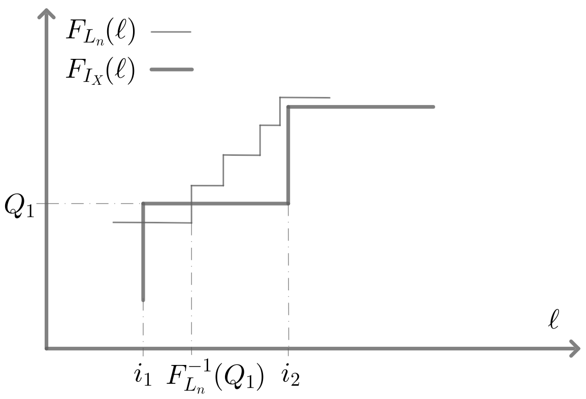
Figure 6: Example section of CDF plots

We can then denote the value of $F_{I_{X}}(l)$ with $i_{1}\leq l<i_{2}$ as $Q_{1}$. If the CDFs cross within this range, this occurs at $l=F_{L_{n}}^{-1}(Q_{1})$. We can write,

$$Q_{1}=\quad\sum_{\mathclap{\begin{subarray}{c}y^{n}\in\mathcal{Y}^{n}:\\ l_{n}(y^{n})<F_{L_{n}}^{-1}(Q_{1})\end{subarray}}}\quad Q_{Y^{n}}(y^{n})+\;\;\alpha\;\sum_{\mathclap{\begin{subarray}{c}y^{n}\in\mathcal{Y}^{n}:\\ l_{n}(y^{n})=F_{L_{n}}^{-1}(Q_{1})\end{subarray}}}\quad Q_{Y^{n}}(y^{n}),$$ (152)

where $0\leq\alpha\leq 1$ is a constant. Consider the $L^{1}$ norm:

$$\int^{l_{\max}}_{l_{\min}}\left|F_{L_{n}}(l)-F_{I_{X}}(l)\right|\mathrm{d}l\geq\int_{i_{1}}^{i_{2}}\left|F_{L_{n}}(l)-F_{I_{X}}(l)\right|\mathrm{d}l$$ (153)

$$=\int_{i_{1}}^{i_{2}}\!\bigg{(}\sum_{y^{n}\in\mathcal{Y}^{n}}Q_{Y^{n}}(y^{n})\mathds{1}[l_{n}(y^{n})\leq l]-Q_{1}\bigg{)}^{+}\mathrm{d}l+\int_{i_{1}}^{i_{2}}\bigg{(}Q_{1}-\!\!\sum_{y^{n}\in\mathcal{Y}^{n}}\!Q_{Y^{n}}(y^{n})\mathds{1}[l_{n}(y^{n})\leq l]\bigg{)}^{+}\mathrm{d}l,$$ (154)

where $(z)^{+}=\max\{z,0\}$. Taking the first term:

$$\int_{i_{1}}^{i_{2}}\bigg{(}\sum_{y^{n}\in\mathcal{Y}^{n}}Q_{Y^{n}}(y^{n})\mathds{1}[l_{n}(y^{n})\leq l]-Q_{1}\bigg{)}^{+}\mathrm{d}l$$

$$=\int_{i_{1}}^{i_{2}}\sum_{y^{n}\in\mathcal{Y}^{n}}Q_{Y^{n}}(y^{n})\big{(}\mathds{1}[l_{n}(y^{n})\leq l]-\mathds{1}\left[l_{n}(y^{n})<F_{L_{n}}^{-1}(Q_{1})\right]-\alpha\>\mathds{1}\left[l_{n}(y^{n})=F_{L_{n}}^{-1}(Q_{1})\right]\big{)}^{+}\mathrm{d}l$$ (155)

$$\geq\int_{i_{1}}^{i_{2}}\sum_{y^{n}\in\widetilde{\mathcal{Y}}^{n}}Q_{Y^{n}}(y^{n})\big{(}\mathds{1}[l_{n}(y^{n})\leq l]-\mathds{1}\left[l_{n}(y^{n})<F_{L_{n}}^{-1}(Q_{1})\right]-\alpha\>\mathds{1}\left[l_{n}(y^{n})=F_{L_{n}}^{-1}(Q_{1})\right]\big{)}^{+}\mathrm{d}l$$ (156)

$$=\int_{i_{1}}^{i_{2}}\sum_{y^{n}\in\widetilde{\mathcal{Y}}^{n}}Q_{Y^{n}}(y^{n})\mathds{1}\left[F_{L_{n}}^{-1}(Q_{1})<l_{n}(y^{n})\leq l\right]\mathrm{d}l$$

$$\qquad\qquad\qquad\qquad\qquad+\int_{i_{1}}^{i_{2}}\sum_{y^{n}\in\widetilde{\mathcal{Y}}^{n}}Q_{Y^{n}}(y^{n})(1-\alpha)\mathds{1}\left[F_{L_{n}}^{-1}(Q_{1})=l_{n}(y^{n})\leq l\right]\mathrm{d}l,$$ (157)

where (155) applies (152), and (156) removes terms for which $y^{n}\notin\widetilde{\mathcal{Y}}^{n}$. Lastly, (157) rearranges the indicator terms. To understand the last step, note that the sum of the three indicator terms in (156) is either $1$ if $F_{L_{n}}^{-1}(Q_{1})<l_{n}(y^{n})\leq l$, $(1-\alpha)$ if $F_{L_{n}}^{-1}(Q_{1})=l_{n}(y^{n})\leq l$, or else non-positive. We proceed with the first term of (157), and say that for $n$ large enough,

$$\int_{i_{1}}^{i_{2}} \sum_{y^{n}\in\widetilde{\mathcal{Y}}^{n}}Q_{Y^{n}}(y^{n})\mathds{1}\left[F_{L_{n}}^{-1}(Q_{1})<l_{n}(y^{n})\leq l\right]\mathrm{d}l$$

$$\geq\int_{i_{1}}^{i_{2}}\sum_{y^{n}\in\widetilde{\mathcal{Y}}^{n}}Q_{Y^{n}}(y^{n})\mathds{1}\left[F_{L_{n}}^{-1}(Q_{1})<l_{n}(y^{n})\right]\mathds{1}\left[l\geq i_{X}(x^{\star}(y^{n}))-\theta_{2}2^{-nK(P_{n})}\right]\mathrm{d}l$$ (158)

$$\geq\sum_{y^{n}\in S^{1}_{i_{2}}}Q_{Y^{n}}(y^{n})\int^{i_{2}}_{i_{1}}\mathds{1}\left[l\geq i_{X}(x^{\star}(y^{n}))-\theta_{2}2^{-nK(P_{n})}\right]\mathrm{d}l$$ (159)

$$=\sum_{y^{n}\in S^{1}_{i_{2}}}Q_{Y^{n}}(y^{n})\min\left\{\theta_{2}2^{-nK(P_{n})},i_{2}-i_{1}\right\},$$ (160)

where

$$S^{1}_{i_{2}}\vcentcolon=\left\{y^{n}\in\widetilde{\mathcal{Y}}^{n}:i_{X}(x^{\star}(y^{n}))=i_{2}\;,\;l_{n}(y^{n})>F_{L_{n}}^{-1}(Q_{1})\right\},$$ (161)

(158) applies Lemma 3 and (159) removes $y^{n}$ terms for which $i_{X}(x^{\star}(y^{n}))\neq i_{2}$. The second term in (157) can be treated identically, giving

$$\int_{i_{1}}^{i_{2}}\sum_{y^{n}\in\widetilde{\mathcal{Y}}^{n}}Q_{Y^{n}}(y^{n})\alpha\mathds{1} \left[l<l_{n}(y^{n})=F_{L_{n}}^{-1}(Q_{1})\right]\mathrm{d}l$$

$$\geq(1-\alpha)\!\!\sum_{y^{n}\in S^{2}_{i_{2}}}Q_{Y^{n}}(y^{n})\min\left\{\theta_{2}2^{-nK(P_{n})},i_{2}-i_{1}\right\},$$ (162)

where

$$S^{2}_{i_{2}}\vcentcolon=\left\{y^{n}\in\widetilde{\mathcal{Y}}^{n}:i_{X}(x^{\star}(y^{n}))=i_{2}\;,\;l_{n}(y^{n})=F_{L_{n}}^{-1}(Q_{1})\right\}.$$ (163)

Returning to (154), we now take the second term.

$$\int_{i_{1}}^{i_{2}}\bigg{(}Q_{1}-\sum_{y^{n}\in\mathcal{Y}^{n}}Q_{Y^{n}}(y^{n})\mathds{1}[l_{n}(y^{n})\leq l]\bigg{)}^{+}\mathrm{d}l$$

$$=\int_{i_{1}}^{i_{2}}\!\!\sum_{y^{n}\in\mathcal{Y}^{n}}Q_{Y^{n}}(y^{n})\big{(}-\mathds{1}[l_{n}(y^{n})\leq l]+\mathds{1}\left[l_{n}(y^{n})<F_{L_{n}}^{-1}(Q_{1})\right]+\alpha\mathds{1}\left[l_{n}(y^{n})=F_{L_{n}}^{-1}(Q_{1})\right]\big{)}^{+}\mathrm{d}l$$ (164)

$$\geq\int_{i_{1}}^{i_{2}}\!\!\sum_{y^{n}\in\widetilde{\mathcal{Y}}^{n}}Q_{Y^{n}}(y^{n})\big{(}-\mathds{1}[l_{n}(y^{n})\leq l]+\mathds{1}\left[l_{n}(y^{n})<F_{L_{n}}^{-1}(Q_{1})\right]+\alpha\mathds{1}\left[l_{n}(y^{n})=F_{L_{n}}^{-1}(Q_{1})\right]\big{)}^{+}\mathrm{d}l$$ (165)

$$=\int_{i_{1}}^{i_{2}}\sum_{y^{n}\in\widetilde{\mathcal{Y}}^{n}}Q_{Y^{n}}(y^{n})\mathds{1}\left[l<l_{n}(y^{n})<F_{L_{n}}^{-1}(Q_{1})\right]\mathrm{d}l$$

$$\qquad\qquad\qquad\qquad\qquad\qquad+\int_{i_{1}}^{i_{2}}\sum_{y^{n}\in\widetilde{\mathcal{Y}}^{n}}Q_{Y^{n}}(y^{n})\alpha\mathds{1}\left[l<l_{n}(y^{n})=F_{L_{n}}^{-1}(Q_{1})\right]\mathrm{d}l$$ (166)

where (164) applies (152), (165) removes terms for which $y^{n}\notin\widetilde{\mathcal{Y}}^{n}$, and (166) rearranges indicator terms. To understand the last step, note that the sum of the three indicator terms in (165) is either $1$ if $l<l_{n}(y^{n})<F_{L_{n}}^{-1}(Q_{1})$, $\alpha$ if $l<l_{n}(y^{n})=F_{L_{n}}^{-1}(Q_{1})$, or else non-positive. We proceed with the first term of (166). If $n$ is large enough,

$$\int_{i_{1}}^{i_{2}} \sum_{y^{n}\in\widetilde{\mathcal{Y}}^{n}}Q_{Y^{n}}(y^{n})\mathds{1}\left[l<l_{n}(y^{n})<F_{L_{n}}^{-1}(Q_{1})\right]\mathrm{d}l$$

$$\geq\int_{i_{1}}^{i_{2}}\sum_{y^{n}\in\widetilde{\mathcal{Y}}^{n}}Q_{Y^{n}}(y^{n})\mathds{1}\left[l_{n}(y^{n})<F_{L_{n}}^{-1}(Q_{1})\right]\mathds{1}\left[l<i_{X}(x^{\star}(y^{n}))-\theta_{1}2^{-nK(P_{n})}\right]\mathrm{d}l$$ (167)

$$\geq\sum_{y^{n}\in S^{3}_{i_{2}}}Q_{Y^{n}}(y^{n})\int^{i_{2}}_{i_{1}}\mathds{1}\left[l<i_{X}(x^{\star}(y^{n}))-\theta_{1}2^{-nK(P_{n})}\right]\mathrm{d}l$$ (168)

$$=\sum_{y^{n}\in S^{3}_{i_{2}}}Q_{Y^{n}}(y^{n})\left(i_{2}-i_{1}-\theta_{1}2^{-nK(P_{n})}\right)^{+},$$ (169)

where

$$S^{3}_{i_{2}}\vcentcolon=\left\{y^{n}\in\widetilde{\mathcal{Y}}^{n}:i_{X}(x^{\star}(y^{n}))=i_{2}\;,\;l_{n}(y^{n})<F_{L_{n}}^{-1}(Q_{1})\right\},$$ (170)

(167) applies Lemma 3 and (168) removes $y^{n}$ terms for which $i_{X}(x^{\star}(y^{n}))\neq i_{2}$. The second term in (166) can be treated identically, giving

$$\int_{i_{1}}^{i_{2}}\sum_{y^{n}\in\widetilde{\mathcal{Y}}^{n}} Q_{Y^{n}}(y^{n})\alpha\mathds{1}\left[l<l_{n}(y^{n})=F_{L_{n}}^{-1}(Q_{1})\right]\mathrm{d}l\geq\alpha\sum_{y^{n}\in S^{2}_{i_{2}}}Q_{Y^{n}}(y^{n})\left(i_{2}-i_{1}-\theta_{1}2^{-nK(P_{n})}\right)^{+}.$$ (171)

Finally combining (160), (162), (169) and (171) we have:

$$\int_{l_{\min}}^{l_{\max}} \left|F_{L_{n}}(l)-F_{I_{X}}(l)\right|\mathrm{d}l$$

$$\geq\sum_{y^{n}\in S^{1}_{i_{2}}}Q_{Y^{n}}(y^{n})\min\left\{\theta_{2}2^{-nK(P_{n})},i_{2}-i_{1}\right\}+\sum_{y^{n}\in S^{3}_{i_{2}}}Q_{Y^{n}}(y^{n})\left(i_{2}-i_{1}-\theta_{1}2^{-nK(P_{n})}\right)^{+}$$

$$\qquad+\sum_{y^{n}\in S_{i_{2}}^{2}}Q_{Y^{n}}(y^{n})\min\left\{\theta_{2}2^{-nK(P_{n})},\left(i_{2}-i_{1}-\theta_{1}2^{-nK(P_{n})}\right)^{+}\right\}$$ (172)

$$\geq\sum_{y^{n}\in S_{i_{2}}}Q_{Y^{n}}(y^{n})\min\left\{\theta_{2}2^{-nK(P_{n})},\left(i_{2}-i_{1}-\theta_{1}2^{-nK(P_{n})}\right)^{+}\right\}$$ (173)

$$=\theta_{2}\sum_{y^{n}\in S_{i_{2}}}Q_{Y^{n}}(y^{n})2^{-nK(P_{n})},$$ (174)

where $S_{i_{2}}$ is the union of $S^{1}_{i_{2}}$, $S^{2}_{i_{2}}$ and $S^{3}_{i_{2}}$, i.e., the set of all sequences $y^{n}\in\widetilde{\mathcal{Y}}^{n}$ such that $i_{X}(x^{\star}(y^{n}))=i_{2}$. We recognise that, for all $y^{n}\in\widetilde{\mathcal{Y}}^{n}$, $\theta_{2}2^{-nK(P_{n})}$ and $\theta_{1}2^{-nK(P_{n})}$ can be made arbitrarily small. In (174) we take $n$ to be large enough that $\theta_{2}2^{-nK(P_{n})}$ is always the minimiser of (173). We next define the domain $D_{i_{2}}$ as follows

$$D_{i_{2}}\vcentcolon=\bigcup_{x:i_{X}(x)=i_{2}}D_{x},$$ (175)

which means that $P_{n}\in\widetilde{\mathcal{P}}_{n}\cap D_{i_{2}}\Rightarrow P_{n}\in S_{i_{2}}$ by Remark 2. Continuing directly from (174) and applying the law of total probability:

$$\int_{l_{\min}}^{l_{\max}} \left|F_{L_{n}}(l)-F_{I_{X}}(l)\right|\mathrm{d}l$$

$$\geq\theta_{2}\sum_{P_{n}\in\widetilde{\mathcal{P}}_{n}\cap{D}_{i_{2}}}\sum_{x^{\prime}}Q_{Y^{n}|X=x^{\prime}}(T(P_{n}))Q_{X}(x^{\prime})2^{-nK(P_{n})}$$ (176)

$$\geq\frac{\theta_{2}\min_{x}Q_{X}(x)}{(n+1)^{|\mathcal{Y}|}}\sum_{P_{n}\in\widetilde{\mathcal{P}}_{n}\cap{D}_{i_{2}}}\sum_{x^{\prime}}2^{-nD(P_{n}||Q_{x^{\prime}})}2^{-nD(P_{n}||Q_{x_{2}(P_{n})})}2^{nD(P_{n}||Q_{x^{\star}})}$$ (177)

$$\geq\frac{\theta_{2}\min_{x}Q_{X}(x)}{(n+1)^{|\mathcal{Y}|}}\sum_{P_{n}\in\widetilde{\mathcal{P}}_{n}\cap{D}_{i_{2}}}2^{-nD(P_{n}||Q_{x_{2}(P_{n})})}$$ (178)

$$\geq\frac{\theta_{2}\min_{x}Q_{X}(x)}{(n+1)^{|\mathcal{Y}|}}2^{-n\inf_{P_{n}\in\widetilde{\mathcal{P}}_{n}\cap{D}_{i_{2}}}D(P_{n}||Q_{x_{2}(P_{n})})},$$ (179)

where in (178) we take only $x^{\prime}=x^{\star}$ terms. Consider the exponent. Firstly, note that $i_{2}$ was arbitrary. We can therefore select $i_{2}$ such that the argument of $\inf_{P_{n}\in\widetilde{\mathcal{P}}_{n}}D(P_{n}||Q_{x_{2}(P_{n})})$ is in $D_{i_{2}}$, i.e.,

$$\inf_{P_{n}\in\widetilde{\mathcal{P}}_{n}\cap{D}_{i_{2}}}D(P_{n}||Q_{x_{2}(P_{n})})=\inf_{P_{n}\in\widetilde{\mathcal{P}}_{n}}D(P_{n}||Q_{x_{2}(P_{n})}).$$ (180)

This, combined with (179) gives

$$\lim_{n\to\infty}\frac{1}{n}\log||F_{L_{n}}-F_{I_{X}}||_{1}\geq-\lim_{n\to\infty}\inf_{P_{n}\in\widetilde{\mathcal{P}}_{n}}D(P_{n}||Q_{x_{2}(P_{n})}).$$ (181)

We can use standard continuity arguments [16, eq. 55] to take the limit of the exponent:

$$\lim_{n\to\infty}\inf_{P_{n}:D(P_{n}||Q_{x_{1}(P_{n})})\leq C_{n}-\frac{1}{\sqrt{n}}}D(P_{n}||Q_{x_{2}(P_{n})}) =\inf_{P:D(P||Q_{x_{1}(P)})\leq C}D(P||Q_{x_{2}(P)})$$

$$\;=C,$$ (182)

since we know that if $\hat{P}$ is the argument of $C$,

$$D(\hat{P}||Q_{x_{1}(\hat{P})})=D(\hat{P}||Q_{x_{2}(\hat{P})})=C,$$ (183)

and $D(P||Q_{x_{2}(P)})$ is a continuous function of $P$. This along with (181) gives

$$\lim_{n\to\infty}\frac{1}{n}\log||F_{L_{n}}-F_{I_{X}}||_{1}\geq-C,$$ (184)

for information theoretic leakage functions with the derivative property. This, combined with (23) proves the equality part of Theorem 2.

VII-D Global Leakage Proofs

We assume throughout that the function $g_{2}(x)$ is infinitely differentiable in its domain and the function $h(\cdot,Q)$ is twice differentiable in its domain with bounded second order partial derivatives. The next statement is analogous to Lemma 3, but expands the function $h(P,Q)$ rather than $f(P,Q)$.

Lemma 6.

For any observation $y^{n}$ whose type $P_{n}\in\widetilde{\mathcal{P}}^{n}$, $h(Q_{X|Y^{n}=y^{n}},Q_{X})$ is bounded by $h(E_{x^{\star}},Q_{X})$ as follows

$$h(E_{x^{\star}},Q_{X})-\theta^{\prime}_{1}2^{-nK(P_{n})}\leq h(Q_{X|Y^{n}=y^{n}},Q_{X})\leq h(E_{x^{\star}},Q_{X})-\theta^{\prime}_{2}2^{-nK(P_{n})}$$ (185)

if $n$ is large enough, where

$$\theta^{\prime}_{1} \vcentcolon=\frac{3\beta^{\prime}}{2\min_{x}Q_{X}(x)},$$ (186)

$$\theta^{\prime}_{2} \vcentcolon=\frac{\gamma^{\prime}}{4}\min_{x}Q_{X}(x),$$ (187)

and $\beta^{\prime},\gamma^{\prime}>0$ are finite constants.

Proof.

The proof is identical to that of Lemma 3, where $f$ is replaced with $h$ and

$$\beta^{\prime} \vcentcolon=-\min_{x\neq x^{\star}}\left(\frac{\partial h(P,Q_{X})}{\partial p_{x}}\Bigg{|}_{P=E_{x^{\star}}}-\frac{\partial h(P,Q_{X})}{\partial p_{x^{\star}}}\Bigg{|}_{P=E_{x^{\star}}}\right),$$ (188)

$$\gamma^{\prime} \vcentcolon=-\max_{x\neq x^{\star}}\left(\frac{\partial h(P,Q_{X})}{\partial p_{x}}\Bigg{|}_{P=E_{x^{\star}}}-\frac{\partial h(P,Q_{X})}{\partial p_{x^{\star}}}\Bigg{|}_{P=E_{x^{\star}}}\right),$$ (189)

are strictly positive by Corollary 4. ∎

VII-D1 Proof of Theorem 3

We use Lemma 6 to prove the upper bound of $\mathcal{L}_{\infty}-\mathcal{L}_{n}$. Many of the steps are are similar to the proof of Lemma 5. First, we consider $\mathbb{E}_{Y^{n}}[g_{1}(l(Y^{n}))]$ :

$$\sum_{y^{n}\in\mathcal{Y}^{n}}Q_{Y^{n}}(y^{n})h(Q_{X|Y^{n}=y^{n}},Q_{X})$$

$$=\sum_{y^{n}\in\widetilde{\mathcal{Y}}^{n}}Q_{Y^{n}}(y^{n})h(Q_{X|Y^{n}=y^{n}},Q_{X})+\sum_{y^{n}\notin\widetilde{\mathcal{Y}}^{n}}Q_{Y^{n}}(y^{n})h(Q_{X|Y^{n}=y^{n}},Q_{X})$$ (190)

$$\geq\sum_{y^{n}\in\widetilde{\mathcal{Y}}^{n}}Q_{Y^{n}}(y^{n})\left(h(E_{x^{\star}},Q_{X})-\theta^{\prime}_{1}2^{-nK(P_{n})}\right)-\max_{P\in\mathcal{P}}|h(P,Q_{X})|\sum_{y^{n}\notin\widetilde{\mathcal{Y}}^{n}}Q_{Y^{n}}(y^{n})$$ (191)

$$\geq\sum_{y^{n}\in\widetilde{\mathcal{Y}}^{n}}Q_{Y^{n}}(y^{n})\left(h(E_{x^{\star}},Q_{X})-\theta^{\prime}_{1}2^{-nK(P_{n})}\right)-\max_{P\in\mathcal{P}}|h(P,Q_{X})|\psi$$ (192)

$$=\sum_{x\in\mathcal{X}}Q_{Y^{n}}(S_{x})h(E_{x},Q_{X})-\sum_{y^{n}\notin\tilde{\mathcal{Y}}^{n}}Q_{Y^{n}}(y^{n})h(E_{x^{*}},Q_{X})$$

$$\qquad\qquad\qquad\qquad\qquad\qquad-\theta^{\prime}_{1}\sum_{x\in\mathcal{X}}\sum_{P_{n}\in\widetilde{\mathcal{P}}_{n}\cap D_{x}}Q_{Y^{n}|X=x}(T(P_{n}))Q_{X}(x)2^{-nK(P_{n})}-\psi^{\prime}$$ (193)

$$\geq\sum_{x\in\mathcal{X}}Q_{Y^{n}}(S_{x})h(E_{x},Q_{X})-\theta^{\prime}_{1}\sum_{x\in\mathcal{X}}\sum_{P_{n}\in\widetilde{\mathcal{P}}_{n}\cap D_{x}}Q_{Y^{n}|X=x}(T(P_{n}))Q_{X}(x)2^{-nK(P_{n})}-2\psi^{\prime}$$ (194)

$$\geq\sum_{x\in\mathcal{X}}\left(Q_{X}(x)h(E_{x},Q_{X})-\phi|h(E_{x},Q_{X})|\right)-\theta^{\prime}_{1}\sum_{x\in\mathcal{X}}\sum_{P_{n}\in\widetilde{\mathcal{P}}_{n}\cap D_{x}}2^{-nD(P_{n}||Q_{x})}2^{-nK(P_{n})}-2\psi^{\prime}$$ (195)

$$\geq\sum_{x\in\mathcal{X}}Q_{X}(x)h(E_{x},Q_{X})-|\mathcal{X}|\phi\max_{x}|h(E_{x},Q_{X})|-\theta^{\prime}_{1}\sum_{x\in\mathcal{X}}\sum_{P_{n}\in\widetilde{\mathcal{P}}_{n}\cap D_{x}}\!\!\!\!2^{-nD(P_{n}||Q_{x})}2^{-nK(P_{n})}-2\psi^{\prime}$$ (196)

where $\psi^{\prime}\vcentcolon=\max_{P\in\mathcal{P}}|h(P,Q_{X})|\psi$, (191) applies Lemma 6, (192) applies Lemma 1, and (195) applies Lemma 4. Consider the third term.

$$\theta^{\prime}_{1}\sum_{x\in\mathcal{X}}\sum_{P_{n}\in\widetilde{\mathcal{P}}_{n}\cap D_{x}} 2^{-nD(P_{n}||Q_{x})}2^{-nK(P_{n})}$$

$$=\theta^{\prime}_{1}\sum_{x\in\mathcal{X}}\sum_{P_{n}\in\widetilde{\mathcal{P}}_{n}\cap D_{x}}2^{-nD(P_{n}||Q_{x})}2^{-nD(P_{n}||Q_{x_{2}(P_{n})})}2^{nD(P_{n}||Q_{x^{\star}})}$$ (197)

$$\leq\theta^{\prime}_{1}|\mathcal{X}|\sum_{P_{n}\in\widetilde{\mathcal{P}}_{n}}2^{-nD(P_{n}||Q_{x_{2}(P_{n})})}$$ (198)

$$\leq\theta^{\prime}_{1}|\mathcal{X}|(n+1)^{|\mathcal{Y}|}2^{-nC_{n}}.$$ (199)

In (198) we recognise that $2^{-nD(P_{n}||Q_{x})}\leq 2^{-nD(P_{n}||Q_{x^{\star}})}$ for any $x\in\mathcal{X}$. We can continue from (196).

$$\sum_{y^{n}\in\mathcal{Y}^{n}} Q_{Y^{n}}(y^{n})h(Q_{X|Y^{n}=y^{n}},Q_{X})$$

$$\geq\sum_{x\in\mathcal{X}}Q_{X}(x)h(E_{x},Q_{X})-|\mathcal{X}|\phi\max_{x}|h(E_{x},Q_{X})|-\theta^{\prime}_{1}|\mathcal{X}|(n+1)^{|\mathcal{Y}|}2^{-nC_{n}}-2\psi^{\prime}.$$ (200)

Now applying $g_{2}$, which is a strictly monotonic increasing function, and employing Taylor’s theorem to expand $g_{2}$ around $\sum_{x\in\mathcal{X}}Q_{X}(x)h(E_{x},Q_{X})$, we get

$$\mathcal{L}_{n}=g_{2}\left(\sum_{y^{n}\in\mathcal{Y}^{n}}Q_{Y^{n}}(y^{n})h(Q_{X|Y^{n}=y^{n}},Q_{X})\right)$$

$$\geq g_{2}\left(\sum_{x\in\mathcal{X}}Q_{X}(x)h(E_{x},Q_{X})-|\mathcal{X}|\phi\max_{x}|h(E_{x},Q_{X})|-\theta^{\prime}_{1}|\mathcal{X}|(n+1)^{|\mathcal{Y}|}2^{-nC_{n}}-2\psi^{\prime}\right)$$ (201)

$$=g_{2}\left(\sum_{x\in\mathcal{X}}Q_{X}(x)h(E_{x},Q_{X})\right)\!-\!\bigg{(}|\mathcal{X}|\phi\max_{x}|h(E_{x},Q_{X})|+\theta^{\prime}_{1}|\mathcal{X}|(n+1)^{|\mathcal{Y}|}2^{-nC_{n}}-2\psi^{\prime}\bigg{)}g^{\prime}_{2}(b),$$ (202)

where $b$ is some value between $\sum_{y^{n}\in\mathcal{Y}^{n}}Q_{Y^{n}}(y^{n})h(Q_{X|Y^{n}=y^{n}},Q_{X})$ and $\sum_{x\in\mathcal{X}}Q_{X}(x)h(E_{x},Q_{X})$. As $g_{2}$ is strictly monotonic increasing, $g^{\prime}_{2}(b)$ is positive. Finally, we can say

$$\lim_{n\to\infty}\frac{1}{n}\log\left(\mathcal{L}_{\infty}-\mathcal{L}_{n}\right)\leq\lim_{n\to\infty}-C_{n}=-C,$$ (203)

where in the equality we have employed Remark 4. We have the upper bound of Theorem 3.

Next, we find the lower bound of $\mathcal{L}_{\infty}-\mathcal{L}_{n}$. We will consider $y^{n}\in\widetilde{\mathcal{Y}}^{n}$ and $y^{n}\notin\widetilde{\mathcal{Y}}^{n}$ separately. Starting with the latter, we use the convexity of $h(P,Q)$ in $P$ to say

$$h(Q_{X|Y^{n}=y^{n}},Q_{X}) \leq\sum_{x\in\mathcal{X}}Q_{X|Y^{n}=y^{n}}(x)h(E_{x},Q_{X}),$$ (204)

and

$$\sum_{y^{n}\notin\widetilde{\mathcal{Y}}^{n}}Q_{Y^{n}}(y^{n})h(Q_{X|Y^{n}=y^{n}},Q_{X}) \leq\sum_{x\in\mathcal{X}}Q_{X}(x)h(E_{x},Q_{X})\sum_{y^{n}\notin\widetilde{\mathcal{Y}}^{n}}Q_{Y^{n}|X=x}(y^{n}),$$ (205)

where the last line takes an average over $y^{n}\notin\widetilde{\mathcal{Y}}^{n}$ and makes use of Bayes’ theorem on the RHS. Moving onto $y^{n}\in\widetilde{\mathcal{Y}}^{n}$, we employ Taylor’s theorem for expanding $h(\cdot,Q_{X})$ around $E_{x}$, $x\in\mathcal{X}$. We then scale each term by $Q_{X|Y^{n}=y^{n}}(x)$ and sum over all $x\in\mathcal{X}$, giving

$$h(Q_{X|Y^{n}=y^{n}} ,Q_{X})$$

$$= \sum_{x\in\mathcal{X}}Q_{X|Y^{n}=y^{n}}(x)h(E_{x},Q_{X})+\sum_{x\in\mathcal{X}}Q_{X|Y^{n}=y^{n}}(x)(Q_{X|Y^{n}=y^{n}}-E_{x})^{\intercal}\nabla h(E_{x},Q_{X})$$

$$+\frac{1}{2}\sum_{x\in\mathcal{X}}Q_{X|Y^{n}=y^{n}}(x)(Q_{X|Y^{n}=y^{n}}-E_{x})^{\intercal}H(\mathbf{b}_{x})(Q_{X|Y^{n}=y^{n}}-E_{x}),$$ (206)

where $\mathbf{b}_{x}$ lies between $Q_{X|Y^{n}=y^{n}}$ and $E_{x}$. Averaging over $y^{n}\in\widetilde{\mathcal{Y}}^{n}$ gives

$$\sum_{y^{n}\in\widetilde{\mathcal{Y}}^{n}}Q_{Y^{n}}(y^{n})h(Q_{X|Y^{n}=y^{n}},Q_{X})$$

$$\quad=\sum_{x\in\mathcal{X}}Q_{X}(x)h(E_{x},Q_{X})\sum_{y^{n}\in\widetilde{\mathcal{Y}}^{n}}Q_{Y^{n}|X=x}(y^{n})$$

$$\quad\quad+\sum_{y^{n}\in\widetilde{\mathcal{Y}}^{n}}Q_{Y^{n}}(y^{n})\sum_{x\in\mathcal{X}}Q_{X|Y^{n}=y^{n}}(x)(Q_{X|Y^{n}=y^{n}}-E_{x})^{\intercal}\nabla h(E_{x},Q_{X})$$

$$\quad\quad+\frac{1}{2}\sum_{y^{n}\in\widetilde{\mathcal{Y}}^{n}}Q_{Y^{n}}(y^{n})\sum_{x\in\mathcal{X}}Q_{X|Y^{n}=y^{n}}(x)(Q_{X|Y^{n}=y^{n}}-E_{x})^{\intercal}H(\mathbf{b}_{x})(Q_{X|Y^{n}=y^{n}}-E_{x}).$$ (207)

Let us examine the second term (the first order term) of (VII-D1).

$$\sum_{y^{n}\in\widetilde{\mathcal{Y}}^{n}}Q_{Y^{n}}(y^{n})\sum_{x\in\mathcal{X}}Q_{X|Y^{n}=y^{n}}(x)(Q_{X|Y^{n}=y^{n}}-E_{x})^{\intercal}\nabla h(E_{x},Q_{X})$$

$$=\sum_{y^{n}\in\widetilde{\mathcal{Y}}^{n}}Q_{Y^{n}}(y^{n})\sum_{x\in\mathcal{X}}Q_{X|Y^{n}=y^{n}}(x)\sum_{x^{\prime}\neq x}Q_{X|Y^{n}=y^{n}}(x^{\prime})\left(\frac{\partial h(P,Q_{X})}{\partial p_{x^{\prime}}}\Bigg{|}_{P=E_{x}}\!\!\!-\frac{\partial h(P,Q_{X})}{\partial p_{x}}\Bigg{|}_{P=E_{x}}\right)$$ (208)

$$\leq-\beta^{\prime}\sum_{y^{n}\in\widetilde{\mathcal{Y}}^{n}}Q_{Y^{n}}(y^{n})\sum_{x\in\mathcal{X}}Q_{X|Y^{n}=y^{n}}(x)\left(1-Q_{X|Y^{n}=y^{n}}(x)\right)$$ (209)

$$\leq-\beta^{\prime}\sum_{y^{n}\in\widetilde{\mathcal{Y}}^{n}}Q_{X}(x^{\star})Q_{Y^{n}|X=x^{\star}}(y^{n})\left(1-Q_{X|Y^{n}=y^{n}}(x^{\star})\right)$$ (210)

$$\leq-\beta^{\prime}\sum_{y^{n}\in\widetilde{\mathcal{Y}}^{n}}Q_{X}(x^{\star})Q_{Y^{n}|X=x^{\star}}(y^{n})\frac{1}{2}\min_{x}Q_{X}(x)2^{-nK(P_{n})}$$ (211)

$$\leq-\frac{\beta^{\prime}\min_{x}Q_{X}(x)^{2}}{2(n+1)^{|\mathcal{Y}|}}\sum_{P_{n}\in\widetilde{\mathcal{P}}_{n}}2^{-nD(P_{n}||Q_{x^{\star}})}2^{-nK(P_{n})}$$ (212)

$$=-\frac{\beta^{\prime}\min_{x}Q_{X}(x)^{2}}{2(n+1)^{|\mathcal{Y}|}}\sum_{P_{n}\in\widetilde{\mathcal{P}}_{n}}2^{-nD(P_{n}||Q_{x_{2}(P_{n})})}$$ (213)

$$\leq-\frac{\beta^{\prime}\min_{x}Q_{X}(x)^{2}}{2(n+1)^{|\mathcal{Y}|}}2^{-n\inf_{P_{n}\in\widetilde{\mathcal{P}}_{n}}D(P_{n}||Q_{x_{2}(P_{n})})},$$ (214)

where in (208) we used (83-85) to expand $(Q_{X|Y^{n}=y^{n}}-E_{x})^{\intercal}\nabla h(E_{x},Q_{X})$, in (209) we apply Corollary 4, in (210) we take only the $X=x^{\star}$ term and use Bayes’ theorem, in (211) we use Lemma 2, and in (214) we take only one term in the summation.

Returning to (VII-D1) we now take the third term (the second order term), which we will bound in a similar fashion to (90-92). Let $\nu^{\prime}$ be a positive constant that is as large as the maximum possible magnitude of any element of the Hessian matrix of $h(\cdot,Q_{X})$, evaluated at any point.

$$\sum_{y^{n}\in\widetilde{\mathcal{Y}}^{n}}Q_{Y^{n}}(y^{n})\sum_{x\in\mathcal{X}}Q_{X|Y^{n}=y^{n}}(x)(Q_{X|Y^{n}=y^{n}}-E_{x})^{\intercal}H(\mathbf{b}_{x})(Q_{X|Y^{n}=y^{n}}-E_{x})$$

$$\leq\nu^{\prime}\sum_{y^{n}\in\widetilde{\mathcal{Y}}^{n}}Q_{Y^{n}}(y^{n})\sum_{x\in\mathcal{X}}Q_{X|Y^{n}=y^{n}}(x)\sum_{\hat{x},x^{\prime}}\big{|}\big{(}Q_{X|Y^{n}=y^{n}}(\hat{x})-E_{x}(\hat{x})\big{)}\big{(}Q_{X|Y^{n}=y^{n}}(x^{\prime})-E_{x}(x^{\prime})\big{)}\big{|}$$ (215)

$$\leq\nu^{\prime}|\mathcal{X}|^{2}\sum_{y^{n}\in\widetilde{\mathcal{Y}}^{n}}Q_{Y^{n}}(y^{n})\sum_{x\in\mathcal{X}}Q_{X|Y^{n}=y^{n}}(x)\max_{x^{\prime}}\big{(}Q_{X|Y^{n}=y^{n}}(x^{\prime})-E_{x}(x^{\prime})\big{)}^{2}$$ (216)

$$\leq\frac{\nu^{\prime}|\mathcal{X}|^{2}}{\min_{x}Q_{X}(x)^{2}}\sum_{y^{n}\in\widetilde{\mathcal{Y}}^{n}}Q_{Y^{n}}(y^{n})\sum_{x\in\mathcal{X}}Q_{X|Y^{n}=y^{n}}(x)2^{-2nK(P_{n})}$$ (217)

$$=\frac{\nu^{\prime}|\mathcal{X}|^{2}}{\min_{x}Q_{X}(x)^{2}}\sum_{x\in\mathcal{X}}Q_{X}(x)\sum_{P_{n}\in\widetilde{\mathcal{P}}_{n}}Q_{Y^{n}|X=x}(T(P_{n}))2^{-2nK(P_{n})}$$ (218)

$$\leq\frac{\nu^{\prime}|\mathcal{X}|^{2}}{\min_{x}Q_{X}(x)^{2}}\sum_{x\in\mathcal{X}}\sum_{P_{n}\in\widetilde{\mathcal{P}}_{n}}2^{-nD(P_{n}||Q_{x})}2^{-2nK(P_{n})}$$ (219)

$$\leq\frac{\nu^{\prime}|\mathcal{X}|^{3}}{\min_{x}Q_{X}(x)^{2}}\sum_{P_{n}\in\widetilde{\mathcal{P}}_{n}}2^{-nD(P_{n}||Q_{x^{\star}})}2^{-2nK(P_{n})}$$ (220)

$$\leq\frac{\nu^{\prime}|\mathcal{X}|^{3}}{\min_{x}Q_{X}(x)^{2}}(n+1)^{|\mathcal{Y}|}\max_{P_{n}\in\widetilde{\mathcal{P}}_{n}}2^{-nD(P_{n}||Q_{x_{2}(P_{n})})}2^{n\left(D(P_{n}||Q_{x^{\star}})-(D(P_{n}||Q_{x_{2}(P_{n})})\right)}$$ (221)

$$\leq\frac{\nu^{\prime}|\mathcal{X}|^{3}}{\min_{x}Q_{X}(x)^{2}}(n+1)^{|\mathcal{Y}|}2^{-n\inf_{P_{n}\in\widetilde{\mathcal{P}}_{n}}D(P_{n}||Q_{x_{2}(P_{n})})}2^{-\sqrt{n}},$$ (222)

where (217) applies Lemma 2 and (222) follows from the definition of $\widetilde{\mathcal{P}}_{n}$. We can now combine results from sets $y^{n}\in\widetilde{\mathcal{Y}}^{n}$ and $y^{n}\notin\widetilde{\mathcal{Y}}^{n}$. Summing (205) and (VII-D1), and substituting (214) and (222) for the first and second order terms respectively gives

$$\sum_{y^{n}\in\mathcal{Y}^{n}}Q_{Y^{n}}(y^{n})h(Q_{X|Y^{n}=y^{n}},Q_{X})$$

$$\leq\sum_{x\in\mathcal{X}}Q_{X}(x)h(E_{x},Q_{X})-\left(\frac{\beta^{\prime}\min_{x}Q_{X}(x)^{2}}{2(n+1)^{|\mathcal{Y}|}}-\frac{\nu^{\prime}|\mathcal{X}|^{3}}{2\min_{x}Q_{X}(x)^{2}}(n+1)^{|\mathcal{Y}|}2^{-\sqrt{n}}\right)\cdot$$

$$\qquad\qquad\qquad\qquad\qquad\qquad\qquad\qquad\qquad\qquad\qquad\qquad\qquad 2^{-n\inf_{P_{n}\in\widetilde{\mathcal{P}}_{n}}D(P_{n}||Q_{x_{2}(P_{n})})}.$$ (223)

As exponential terms decay quicker than polynomials, it must eventually be that

$$\frac{1}{2}\frac{\beta^{\prime}\min_{x}Q_{X}(x)^{2}}{2(n+1)^{|\mathcal{Y}|}}\geq\frac{\nu^{\prime}|\mathcal{X}|^{3}}{2\min_{x}Q_{X}(x)^{2}}(n+1)^{|\mathcal{Y}|}2^{-\sqrt{n}}.$$ (224)

Thus we can say that if $n$ is large enough,

$$\sum_{y^{n}\in\mathcal{Y}^{n}}\!\!Q_{Y^{n}}(y^{n}) h(Q_{X|Y^{n}=y^{n}},Q_{X})$$

$$\quad\leq\sum_{x\in\mathcal{X}}Q_{X}(x)h(E_{x},Q_{X})-\frac{\beta^{\prime}\min_{x}Q_{X}(x)^{2}}{4(n+1)^{|\mathcal{Y}|}}2^{-n\inf_{P_{n}\in\widetilde{\mathcal{P}}_{n}}D(P_{n}||Q_{x_{2}(P_{n})})}.$$ (225)

Just as in (VII-D1), we can use Taylor’s theorem to expand $g_{2}$ around $\sum_{x\in\mathcal{X}}Q_{X}(x)h(E_{x},Q_{X})$, retaining the exponential terms. Doing so gives

$$\mathcal{L}_{n} =g_{2}\left(\sum_{y^{n}\in\mathcal{Y}^{n}}Q_{Y^{n}}(y^{n})h(Q_{X|Y^{n}=y^{n}},Q_{X})\right)$$

$$\leq g_{2}\left(\sum_{x\in\mathcal{X}}Q_{X}(x)h(E_{x},Q_{X})-\frac{\beta^{\prime}\min_{x}Q_{X}(x)^{2}}{4(n+1)^{|\mathcal{Y}|}}2^{-n\inf_{P_{n}\in\widetilde{\mathcal{P}}_{n}}D(P_{n}||Q_{x_{2}(P_{n})})}\right)$$ (226)

$$=g_{2}\left(\sum_{x\in\mathcal{X}}Q_{X}(x)h(E_{x},Q_{X})\right)-\frac{\beta^{\prime}\min_{x}Q_{X}(x)^{2}}{4(n+1)^{|\mathcal{Y}|}}2^{-n\inf_{P_{n}\in\widetilde{\mathcal{P}}_{n}}D(P_{n}||Q_{x_{2}(P_{n})})}g^{\prime}_{2}(b),$$ (227)

where $b$ is some value between $\sum_{x\in\mathcal{X}}Q_{X}(x)h(E_{x},Q_{X})$ and $\sum_{y^{n}\in\mathcal{Y}^{n}}Q_{Y^{n}}(y^{n})h(Q_{X|Y^{n}=y^{n}},Q_{X})$ and $g_{2}^{\prime}(b)$ must be positive as $g_{2}$ is strictly monotonic increasing. It follows that

$$\lim_{n\to\infty}\frac{1}{n}\log\left(\mathcal{L}_{\infty}-\mathcal{L}_{n}\right) \geq\lim_{n\to\infty}-\inf_{P_{n}\in\widetilde{\mathcal{P}}_{n}}D(P_{n}||Q_{x_{2}(P_{n})})$$ (228)

$$=\lim_{n\to\infty}-C_{n}=-C,$$ (229)

where the last line makes use of (VII-C2) and Remark 4 in turn. This, combined with (203) completes the proof of Theorem 3.

References

- [1] C. Dwork, “Differential privacy,” in Proc. Int. Colloq. Autom. Lang. Program. (ICALP) (Lecture Notes in Computer Science), vol. 4052. Springer Berlin Heidelberg, 2006, pp. 1–12.
- [2] J. Tang, A. Korolova, X. Bai, X. Wang, and X. Wang, “Privacy Loss in Apple’s Implementation of Differential Privacy on MacOS 10.12,” 2017, arXiv: 1709.02753.
- [3] N. Fernandes, A. McIver, and P. Sadeghi, “Explaining epsilon in local differential privacy through the lens of quantitative information flow,” in Proc. IEEE Comput. Secur. Found. Symp. (CSF), Enschede, Netherlands, Jul. 2024, pp. 419–432. [Online]. Available: https://doi.ieeecomputersociety.org/10.1109/CSF61375.2024.00012
- [4] M. S. Alvim, K. Chatzikokolakis, C. Palamidessi, and G. Smith, “Measuring information leakage using generalized gain functions,” in Proc. IEEE Comput. Secur. Found. Symp. (CSF), Cambridge, MA, USA, Jun. 2012, pp. 265–279.
- [5] M. S. Alvim, K. Chatzikokolakis, A. Mciver, C. Morgan, C. Palamidessi, and G. Smith, “Additive and multiplicative notions of leakage, and their capacities,” in Proc. IEEE Comput. Secur. Found. Symp. (CSF), Vienna, Austria, Jul. 2014, pp. 308–322.
- [6] I. Wagner and D. Eckhoff, “Technical privacy metrics: A systematic survey,” 2015, arXiv: 1512.00327.
- [7] I. Issa, A. B. Wagner, and S. Kamath, “An operational approach to information leakage,” IEEE Trans. Inf. Theory, vol. 66, no. 3, pp. 1625–1657, Mar. 2020.
- [8] B. Rassouli and D. Gündüz, “Optimal utility-privacy trade-off with total variation distance as a privacy measure,” IEEE Trans. Inf. Forensics Secur., vol. 15, pp. 594–603, Mar. 2020.
- [9] S. Saeidian, G. Cervia, T. J. Oechtering, and M. Skoglund, “Pointwise maximal leakage,” IEEE Trans. Inf. Theory, vol. 69, no. 12, p. 8054–8080, Dec. 2023.
- [10] B. Wu, A. B. Wagner, I. Issa, and G. E. Suh, “Strong asymptotic composition theorems for mutual information measures,” IEEE Trans. Inf. Theory, vol. 70, no. 5, pp. 3049–3058, May 2024.
- [11] P. Kairouz, S. Oh, and P. Viswanath, “The composition theorem for differential privacy,” IEEE Trans. Inf. Theory, vol. 63, no. 6, pp. 4037–4049, Jun. 2017.
- [12] T. M. Cover and J. A. Thomas, Elements of Information Theory. USA: Wiley-Interscience, 2006.
- [13] R. Sibson, “Information radius,” Zeitschrift für Wahrscheinlichkeitstheorie und Verwandte Gebiete, vol. 14, no. 2, pp. 149–160, Jun. 1969.
- [14] S. Verdú, “-mutual information,” in Proc. IEEE Inf. Theory and Appl. Workshop (ITA), San Diego, CA, USA, Feb. 2015, pp. 1–6.
- [15] J. Liao, O. Kosut, L. Sankar, and F. du Pin Calmon, “Tunable measures for information leakage and applications to privacy-utility tradeoffs,” IEEE Trans. Inf. Theory, vol. 65, no. 12, pp. 8043–8066, Dec. 2019.
- [16] B. Wu, A. B. Wagner, G. E. Suh, and I. Issa, “Strong asymptotic composition theorems for sibson mutual information,” 2020, arXiv: 2005.06033.