A general condition for bias attenuation by a nondifferentially mismeasured confounder

Abstract

In real-world studies, the collected confounders may suffer from measurement error. Although mismeasurement of confounders is typically unintentional—originating from sources such as human oversight or imprecise machinery—deliberate mismeasurement also occurs and is becoming increasingly more common. For example, in the 2020 U.S. Census, noise was added to measurements to assuage privacy concerns. Sensitive variables such as income or age are oftentimes partially censored and are only known up to a range of values. In such settings, obtaining valid estimates of the causal effect of a binary treatment can be impossible, as mismeasurement of confounders constitutes a violation of the no unmeasured confounding assumption. A natural question is whether the common practice of simply adjusting for the mismeasured confounder is justifiable. In this article, we answer this question in the affirmative and demonstrate that in many realistic scenarios not covered by previous literature, adjusting for the mismeasured confounders reduces bias compared to not adjusting.

1 Introduction

In observational studies, researchers often only have access to mismeasured versions of the true confounders, rendering unbiased estimation of causal effects impossible without additional assumptions. Nevertheless, the observed mismeasured version of the true confounder can be utilized in various ways. One typical assumption on the mismeasured confounder is that it is independent of all other variables conditional on the true confounder. The conventional wisdom has been that adjusting for such an observed but mismeasured confounder leads to less bias than no adjustment whatsover (Greenland,, 1980), and there are now many analytical results that rigorously verify the conventional wisdom under certain assumptions. This problem is well-studied in the statistical literature, and the observed variable is often referred to as a nondifferentially mismeasured confounder. Ogburn and Vanderweele, (2013) study the case of ordinal unmeasured confounders, Gabriel et al., (2022) studies dichotomization of continuous unmeasured confounders, Ogburn and VanderWeele, (2012), Peña, (2020), and Sjölander et al., (2022) study binary unmeasured confounders, and Peña et al., (2021) studies general discrete unmeasured confounders. Each of the above papers provides sufficient conditions or examples/counterexamples of when the estimate of a causal effect adjusting for the observed mismeasured confounder comes closer to the true causal effect than when using the crude, unadjusted estimate. In this paper, we present an interpretable sufficient condition for ordinal and continuous confounders to reduce bias, with no restriction on the support of the unmeasured and mismeasured confounders. In a different vein, Ding et al., (2017) demonstrate that adjusting for an instrumental variable can amplify bias, under some general conditions. We draw on this work to develop our results tailored to our setting.

Also related to our work is the vast literature on auxiliary variables with special causal structure. Such variables should be correlated with unmeasured confounders, and examples include negative control outcomes, negative control exposures, and second treatments. These variables possess qualitative similarities with the mismeasured confounders that we study and have been used for many purposes. Rosenbaum, (1989) and Lipsitch et al., (2010) use negative controls to detect bias, Rosenbaum, (2006) and Chen et al., (2023) use second treatments to learn about differential effects, and the proximal causal inference literature utilizes negative control outcomes, exposures and/or mismeasured versions of confounders to obtain consistent effect estimates or bounds (Tchetgen Tchetgen,, 2014; Kuroki and Pearl,, 2014; Miao et al.,, 2018; Park et al.,, 2024; Ghassami et al.,, 2023). The proxy literature, however, requires assumptions on the variability of the true confounder compared to the proxy. In the discrete case, if the unmeasured confounder has more levels than the proxy, the proxy methodology cannot be applied. We tackle the less ambitious goal of decreasing bias by imposing interpretable monotonicity assumptions but do not restrict the variability of the unmeasured confounder relative to its measured counterpart.

Figure 1: The relationships between treatment $A$, unmeasured confounder $U$ and its mismeasured version $C$, and outcome $Y$.

2 Background and Notation

In our setting, $U$ is an unmeasured, univariate variable that confounds the relationship between a binary treatment $A$ and outcome $Y$. However, we measure an imperfect proxy for $U$, call it $C$, such that $C$ is only affected by $U$. Thus, $A\perp\!\!\!\perp C\mid U$ and $Y\perp\!\!\!\perp C\mid A,U$. For a directed acyclic graph depiction, see Figure 1. We will refer to $C$ as a proxy or mismeasured confounder throughout the manuscript. For ease of exposition, we omit measured confounders $X$, keeping in mind that they can be straightforwardly accommodated with a slight adjustment of the assumptions. All of our assumptions can be interpreted as conditional on $X=x$, and would need to hold for all $x$. We assume the existence of potential outcomes $Y(1)$ and $Y(0)$ that correspond to the outcome that would have been observed if, possibly contrary to fact, a subject had received treatment $A=1$ and $A=0$, respectively. The vector $(U,C,A,Y(1),Y(0))$ is assumed to be sampled iid from an unknown distribution $F$. $f(a)$ will denote the density or probability mass function of a random variable $A$ evaluated at $a$, and $f(a\mid b)$ the density conditional on $B=b$. $\mathcal{A}$ will denote the support of a random variable $A$. We will study whether the unadjusted estimate is more or less biased than the adjusted for $C$ estimate for the true effect.

3 Qualitative similarity between the mismeasured and unmeasured confounder

3.1 Assumptions

We first introduce the causal assumptions needed so that had $U$ been measured, the causal quantities of interest would be identified.

Assumption 1 (Causal assumptions).

(i) $Y=Y(1)A+Y(0)(1-A)$, (ii) For some $\epsilon>0$, $\epsilon\leq P(A=1\mid U=u)\leq 1-\epsilon$ for all $u$, (iii) $\{Y(1),Y(0)\}\perp\!\!\!\perp A\mid U$.

Under these causal assumptions, it is well known that $E(Y(a))$ is identified by $\int E(Y\mid A=a,u)dF(u)=E[AY/P(A=1\mid U)]$. We will require some assumptions on the outcome regressions $E(Y\mid A=a,u)$ and propensity score $P(A=1\mid u)$, which may need to be verified for a posited $U$ through subject matter expertise. Similar assumptions have also been invoked in VanderWeele, (2008), Chiba, (2009),Ogburn and VanderWeele, (2012),Ogburn and Vanderweele, (2013), and Ding et al., (2017).

Assumption 2 (Monotonicity).

We require the following conditions:

1. (outcome regression monotonicity) $E(Y\mid A=a,U=u)$ is non-decreasing in $u$ for $a=0,1$.

2. (propensity score monotonicity) $P(A=1\mid U=u)$ is non-decreasing in $u$.

Remark.

Though we have presented the assumptions in terms of non-decreasing monotonicity, the main attenuation result will continue to hold if one or both montonicity assumptions are flipped to non-increasing.

The next assumption formally encapsulates the assumptions implied by the directed acyclic graph in Figure 1, and is typically referred to as nondifferential mismeasurement (Ogburn and VanderWeele,, 2012).

Assumption 3 (Nondifferential mismeasurement).

$C\perp\!\!\!\perp(A,Y)\mid U$.

The next two assumptions are the most crucial. They impose specific forms of positive dependence between the unmeasured confounder and the measured $C$. Before laying out the assumptions, we introduce two definitions.

Definition 1 (Lehmann, (1966)).

We say that a random variable $A$ is positively (resp. negatively) regression dependent on $B$ if $P(A\geq a\mid B=b)$ is non-decreasing (resp. non-increasing) in $b$ for all $a\in\mathcal{A}$. If $P(A\geq a\mid B=b,C=c)$ is non-decreasing (resp. non-increasing) in $b$ for all $a\in\mathcal{A}$, we say $A$ is positively (resp. negatively) regression dependent on $B$ given $C=c$.

Definition 2 (Karlin and Rubin, (1956); Lehmann, (1966)).

Let $a,a^{\prime}\in\mathcal{A}$ and $b,b^{\prime}\in\mathcal{B}$. We say that a random variable $A$ has positive (resp. negative) likelihood ratio dependence on $B$ if $f(a^{\prime}\mid b^{\prime})f(a\mid b)\geq(\text{resp.}\leq)f(a\mid b^{\prime})f(a^{\prime}\mid b)$ when $a^{\prime}>a,b^{\prime}>b$. If $f(a^{\prime}\mid b^{\prime},c)f(a\mid b,c)\geq(\text{resp.}\leq)f(a\mid b^{\prime},c)f(a^{\prime}\mid b,c)$ when $a^{\prime}>a,b^{\prime}>b$, we say that $A$ has positive (resp. negative) likelihood ratio dependence on $B$ given $C=c$.

The first of the two assumptions is based on regression dependence.

Assumption 4 (Regression Dependence).

(i) $U$ is positive (negative) regression dependent on $C$, (ii) $U$ is positive (negative) regression dependent on $C$ given $A=a$, for $a=0,1$.

Part (i) is relatively easy to interpret, though it places restrictions on $U\mid C$ rather than $C\mid U$. Part (ii) requires that further conditioning on the treatment status does not break the regression dependence, which is harder to interpret. Under the special case where $U$ is binary, part (ii) of Assumption 4 is implied by part (i) when the mismeasurement is nondifferential. This is stated formally below:

Lemma 1.

If $U$ is binary, $C\perp\!\!\!\perp A\mid U$ as in Assumption 3, and Assumption 4(i) holds, then Assumption 4(ii) holds.

The second of the two assumptions is based on likelihood ratio dependence.

Assumption 5 (Monotone likelihood ratio dependence).

$C$ has positive or negative likelihood ratio dependence on $U$.

Assumption 5 turns out to be a stronger assumption than 4 when the mismeasurement is nondifferential, which we formalize in the next proposition. Although it is stronger than 4, assumption 5 is attractive in that it places a restriction on the distribution of $C\mid U$, which is more natural than reasoning about the three distributions $U\mid C$, $U\mid A=1,C$, and $U\mid A=0,C$.

Proposition 1.

If $C\perp\!\!\!\perp A\mid U$ as in Assumption 3, then Assumption 5 implies Assumption 4.

Remark.

Although we have presented the assumptions 4 and 5 allowing either positive or negative dependence, in our proofs we focus on the positive case without loss of generality. In practice, we would expect $C$ to be positively dependent on $U$.

We now verify that the relationship between the mismeasured $C$ and the treatment and outcome is qualitatively similar to that of $U$. This result was derived for binary confounders in Ogburn and VanderWeele, (2012) and Sjölander et al., (2022).

Lemma 2.

Under the positive sign versions of assumptions 2 and 4, and assumption 3,

$$P(A=1\mid C=c),\ E(Y\mid A=0,C=c),\ E(Y\mid A=1,C=c)\text{ are non-decreasing in }c.$$

Equipped with this lemma, we can proceed to the main attenuation result.

4 Main Result

We first introduce a helpful lemma that has been invoked in the previous literature.

Lemma 3 (Esary et al., (1967), Theorem 3.1).

Let $f(\cdot)$ and $g(\cdot)$ be functions, each with $K$ real-valued arguments, which are both non-decreasing in each of their arguments. If $U=\left(U_{1},\ldots,U_{K}\right)$ is a multivariate random variable with $K$ mutually independent components, then $\operatorname{cov}\{f(U),g(U)\}\geq 0$.

The next two lemmas determine the direction of the bias of the adjusted mean compared to the true counterfactual mean as well as the relationship between the unadjusted and adjusted means.

Lemma 4.

Under assumptions 1, the positive sign versions of 2, and 3,

$$\int E(Y\mid A=1,C=c)f(c)dc\geq E[Y(1)]\text{ and }\int E(Y\mid A=0,C=c)f(c)dc\leq E[Y(0)].$$

Lemma 5.

Under the positive sign versions of assumptions 2, 4, and 3,

$$E(Y\mid A=1)\geq\int E(Y\mid A=1,C=c)f(c)dc\text{ and }E(Y\mid A=0)\leq\int E(Y\mid A=0,C=c)f(c)dc.$$

The bias attenuation property then immediately follows from the two previous lemmas.

Theorem 1.

Let $\mu_{a}^{\text{unadj}}=E(Y\mid A=a)$ and $\mu_{a}^{\text{adj}}=\int E(Y\mid A=a,C=c)f(c)dc$ for $a=0,1$, and let $h,g$ be any non-decreasing functions. Under assumptions 1, the positive sign versions of 2, 3, and the positive sign version of 4 or 5,

$$h[g\{\mu_{1}^{\text{unadj}}\}-g\{\mu_{0}^{\text{unadj}}\}]\geq h[g\{\mu_{1}^{\text{adj}}\}-g\{\mu_{0}^{\text{adj}}\}]\geq h[g\{E[Y(1)]\}-g\{E[Y(0)]\}].$$ (1)

Proof.

Lemmas 4 and 5 imply that $\mu_{1}^{\text{unadj}}\geq\mu_{1}^{\text{adj}}\geq E[Y(1)]$ and $-\mu_{0}^{\text{unadj}}\geq-\mu_{0}^{\text{adj}}\geq-E[Y(0)]$ when 1-4 hold. Applying the function $g$ to all quantities, adding them together, and then applying $h$ implies the result. We can swap Assumptions 5 and 4 since the former implies the latter under assumption 3 by Proposition 1. ∎

Remark.

We make several comments. First, when the signs of the monotonicity of the outcome regression and propensity score in Assumption 2 are both non-increasing rather than non-decreasing in $u$, Equation 1 continues to hold. If one is non-increasing while the other is non-decreasing, the inequalities in Equation 1 must be flipped, but attenuation continues to hold. Second, for different choices of $g$ and $h$, Theorem 1 implies attenuation on the difference, ratio, and odds ratio effect scales. Third, in the supplementary material, we demonstrate that attenuation holds for the effect on the treated. Also, similar to Ogburn and Vanderweele, (2013) and Ding et al., (2017), if the unmeasured confounder $U$ is multivariate with independent components, and the monotonicity conditions hold for each component of $U$, attenuation will hold. Finally, we point out that Assumptions 2-4 together have testable implications. Namely, that $P(A=1\mid C=c)$ and $E(Y\mid A=a,C=c)$ are non-decreasing in $c$, and that $\mu_{1}^{\text{adj}}\leq\mu_{1}^{\text{unadj}}$ and $\mu_{0}^{\text{unadj}}\leq\mu_{0}^{\text{adj}}$.

5 Examining Assumptions 4 and 5

The utility of Theorem 1 rests entirely on the plausibility and interpretability of assumptions 4 and 5. Assumptions 4 and 5 are classical notions of positive dependence of random variables, and the former is often invoked in the multiple testing literature as a sufficient condition for false discovery rate control (Benjamini and Yekutieli,, 2001). However, of the assumptions required to establish Theorem 1, 4 and 5 are the hardest to interpret. First, for Assumption 4, a structural causal model in the spirit of Pearl, (2009) (and as displayed in Figure 1) would posit $U$ having a direct influence or arrow into $C$, not vice versa. The condition that $P(C\geq c\mid U=u)$ is non-decreasing in $u$ would be quite natural, but is not equivalent to Assumption 4 in general. Through the next three propositions, we provide one specific but common situation under which Assumption 4 holds, and two general settings under which 5 holds, which, as the reader may recall, implies Assumption 4 under Assumption 3. Then, we provide several examples that fall under these general settings.

Proposition 2 ($C$ non-decreasing in $U$ model).

Suppose $C=\chi(U)$ where $\chi(u)$ is some deterministic function that is non-decreasing in $u$. Then Assumption 4 holds. Moreover, if $C^{*}=\chi^{*}(C)$ for some $C$ that satisfies Assumption 4 and $\chi^{*}$ non-decreasing, then Assumption 4 holds for $C^{*}$ as well.

Proposition 3 (Log-concave additive noise, Example 12 in Lehmann, (1966)).

Suppose $C=U+\epsilon$, where $\epsilon$ is random noise that is independent of $U$. If $f_{\epsilon}$, the density of $\epsilon$, is log-concave, then Assumption 5 holds.

Proposition 4 (Exponential families, Borges and Pfanzagl, (1963)).

Suppose the conditional density of $C\mid U$ follows $f(c\mid u)=h(c)\exp(\eta(u)\times T(c)-A(u))$, where $\eta$ is a non-decreasing function and $T$ is a strictly increasing function. Then Assumption 5 holds.

All of the scenarios in the previous three propositions place realistic and interpretable restrictions on the distribution $C\mid U$. Importantly, in constrast to previous work, they place no restrictions on the distribution or support of $U$. The main distinction between the conditions is that the latter condition imposes a distributional restriction, while the first two impose almost-sure restrictions. Thus, the first two are more amenable to the case where $C$ is truly a mismeasured version of $U$, while the latter is also amenable to the case where $C$ is a negative control outcome or treatment known to be correlated with $U$. Although we have outlined very general conditions under which attenuation will be satisfied, it is instructive to look a few specific examples, some of which have been discussed in previous works on bias attenuation. Detailed justification for each example is contained in the supplementary material.

Example 1 (Normal-Normal).

Suppose $(U,C)$ are bivariate normal and standard normals marginally, with correlation $\rho>0$. This situation satisfies Assumption 5.

Example 2 (Binary-Binary).

Suppose $U,C$ are binary. Then Assumptions 4 and 5 hold if $U$ and $C$ are nonnegatively correlated. If they are negatively correlated, then non-increasing versions of Assumptions 4 and 5 hold. The reasoning was discussed in the remark following Proposition 1. This case was originally investigated in Ogburn and VanderWeele, (2012).

Example 3 (Binary Regression).

Suppose $U\sim F$ and $C\mid U$ either follows a probit or logistic regression. This is a special case of the exponential family, so Assumption 5 is satisfied.

Example 4 (Additive Noise Differential Privacy).

To satisfy certain privacy constraints, independent noise is often added to the true measurements, such as in the 2020 U.S. Census. Two of the most common mechanisms are additive Gaussian and Laplacian noise (Dwork and Roth,, 2013). Both the Gaussian and Laplacian densities are log-concave, so Assumption 5 is satisfied.

Example 5 (Coarsened/Binned Variable).

Suppose $U\sim F$ comes from some unknown distribution $F$ and $C$ has $K$ levels. Suppose $\mu_{k}<\mu_{k+1}$ are some fixed numbers for all $k=1,\ldots,K-1$ and $\mu_{0}$ and $\mu_{K}$ are the essential infimum and supremums of $U$. If $C=k$ when $U\in[\mu_{k-1},\mu_{k}]$, then $C$ is a non-decreasing function of $U$, so Assumption 4 holds. This scenario is common in practice. Continuous confounders like age, education, or income are often binned into ranges. When $K=2$, $C=\mathbbm{1}\{U>\theta\}$ for some threshold $\theta$, which was investigated in Gabriel et al., (2022) under specific models for the unmeasured confounder $U$.

The latter two examples correspond to situations where $C$ is a mismeasured version of $U$, whereas for the previous three, $C$ could plausibly be a proxy of $U$, such as a negative control outcome or exposure. In the next section, we compare our results to those from the previous literature.

6 A closer comparison to previous literature

6.1 Binary $U$, Binary $C$

We have given an alternative proof that demonstrates that for any binary unmeasured confounder $U$ and nondifferentially mismeasured $C$, adjusting for $C$ attenuates the bias when Assumption 2 holds. Such results were originally obtained in Ogburn and VanderWeele, (2012) using a different proof strategy. Additional attenuation results for this scenario without assuming Assumptions 2 were derived in Peña, (2020).

6.2 A dichotomized unmeasured confounder

We have generalized results from Gabriel et al., (2022), who considered a dichotomized confounder under specific distributions of $U\mid A$ and outcome models $E(Y\mid A,U)$. We have shown that under Assumption 2, when $C$ is a binned version of $U$, attenuation holds. Besides providing some specific examples of when attenuation by dichotomization is guaranteed, Gabriel et al., (2022) also wrote down several counterexamples of when dichotomization fails to attenuate bias. In the supplementary material, we examine those counterexamples and demonstrate that in all cases, either Assumption 2 (i) or (ii) fails to hold.

6.3 Ordinal $U$ and $C$

Although Assumptions 4 and 5 apply to ordinal unmeasured confounders, the connection between these assumptions and the tapered distribution assumption introduced in Ogburn and Vanderweele, (2013) is not obvious. In this subsection, we investigate the relationships between the assumptions. Suppose $U$ and $C$ are both ordinal with $K$ levels, labeled $1,\ldots,K$ without loss of generality. We state the tapered assumption from Ogburn and Vanderweele, (2013) below.

Assumption 6 (Tapered misclassification - Ogburn and Vanderweele, (2013)).

Let $p_{ij}=P(C=i\mid U=j)$. The misclassification probabilities are tapered, which means that when $j\leq k\leq i$, $p_{ij}\leq p_{ik}$ and $p_{ji}\leq p_{ki}$, and when $i\leq j\leq k$, and $p_{ij}\geq p_{ik}$ and $p_{ji}\geq p_{ki}$.

Borrowing the language of Ogburn and Vanderweele, (2013), Assumption 6 “means that the probability of correct classification is at least as great as the probability of misclassification into any one level and that, for a fixed level $i$ of either $C$ or $U$, the misclassification probabilities are non-increasing in each direction away from $i$.” This means that viewing the $p_{ij}$ as entries of a matrix, starting at a diagonal entry $p_{ii}$, the probabilities decrease as you move away from $p_{ii}$ horizontally and vertically in either direction. One notable difference between the tapered property and positive regression or monotone likelihood ratio dependence is that the latter two are automatically satisfied if $C$ is independent of $U$ whereas the former is not. We now state a result relating Assumption 6 to the flipped version of Assumption 4(i).

Proposition 5.

Let $U$ and $C$ be ordinal with $K$ levels, and suppose Assumption 6 holds. Then $P(C\geq i\mid U=j)$ is non-decreasing in $j$. In other words, tapered misclassification implies $C$ is positive regression dependent on $U$.

Interestingly, the proof we present is valid if $P_{C\mid U}$ is tapered only in the horizontal direction (Wang and Gustafson,, 2014), which means when $j\leq k\leq i$, $p_{ij}\leq p_{ik}$, and when $i\leq j\leq k$, $p_{ij}\geq p_{ik}$. Although Proposition 5 uncovers a nice connection between tapered misclassification and positive regression dependence, the positive regression dependence from Assumption 4(i) is in the opposite direction. Unlike monotone likelihood ratio dependence, positive regression dependence and tapered misclassification are not symmetric properties. Figure 2 displays the relationships between the three notions of dependence for ordinal variables in a Venn diagram. We give examples of all four possibilities in the supplementary material. For ordinal variables, there exist distributions $C\mid U$ that satisfy Assumptions 4 and/or 5 but not Assumption 6, and vice versa. Therefore, though our assumptions do not generalize the tapered assumption, we have expanded the set of ordinal distributions $C\mid U$ for which attenuation rigorously holds.

Figure 2: A Venn diagram outlining the relationships between tapered (Taper), positively regression dependent (PRD), and positive monotone likelihood ratio dependent (MLR) distributions. The star indicates that MLR is a symmetric property.

One case that our results do not directly apply to is when $U$ and $C$ are discrete with more than two levels, but with no ordering, as studied in Peña et al., (2021). This is because our dependence assumptions require $U$ and $C$ to have natural orderings.

7 Discussion

Adjusting for a nondifferentially mismeasured confounder is conventional wisdom that is practiced widely. Previous analytic results demonstrate that the conventional wisdom is justified in several realistic settings. We have substantially expanded the set of scenarios where the conventional wisdom is justified, including for additive noise and coarsening. Promising future directions would be to obtain similarly general results when the measurement error is not non-differential. Another question is whether general attenuation results can be obtained for all continuous linear functionals of $E(Y\mid A,X)$ by imposing a monotonicity assumption on the Riesz representer of the functional.

Appendix A Proofs of results from Section 3

A.1 Proof of Lemma 1

Proof of Lemma 1.

Since $U$ is binary, we only need to check whether $P(U=1\mid A=1,C=c)$ is increasing in $c$. Observe that by definition and Assumption 3,

$$P(U=1\mid A=1,C=c)$$

$$=\frac{P(A=1\mid U=1,C=c)P(U=1\mid C=c)}{P(A=1\mid U=1,C=c)P(U=1\mid C=c)+P(A=1\mid U=0,C=c)P(U=0,C=c)}$$

$$=\frac{P(A=1\mid U=1)P(U=1\mid C=c)}{P(A=1\mid U=1)P(U=1\mid C=c)+P(A=1\mid U=0)P(U=0\mid C=c)}$$

$$=\frac{al(c)}{al(c)+b(1-l(c))},$$

where we set $a=P(A=1\mid U=1)$, $b=P(A=1\mid U=0)$, and $l(c)=P(U=1\mid C=c)$. All three quantities lie between 0 and 1. Fix some $c^{\prime}>c$. $l(c)$ increases in $c$, so going from $\frac{al(c)}{al(c)+b(1-l(c))}$ to $\frac{al(c^{\prime})}{al(c^{\prime})+b(1-l(c^{\prime}))}$ increasing the numerator by $a[l(c^{\prime})-l(c)]\geq 0$, but the denominator by changes by $a[l(c^{\prime})-l(c)]+b[l(c)-l(c^{\prime})]\leq a[l(c^{\prime})-l(c)]$. Of course, the entire quantity $\frac{al(c)}{al(c)+b(1-l(c))}\leq 1$, so adding a number to the numerator and adding a smaller number to the denominator must increase its value. The argument for the $A=0$ case is identical; just replace $a$ with $P(A=0\mid U=1)$ and $b$ with $P(A=0\mid U=0)$. ∎

A.2 Proof of Proposition 1

Before proceeding to the proof of Proposition 1, we state two simple lemmas that we believe to be well-known.

Lemma A.1.

If Assumption 5 holds for $C\mid U$, it also holds for $U\mid C$.

Lemma A.2.

If Assumption 5 holds for $C\mid U$, then $P(C\geq c\mid U=u)$ is increasing in $u$.

Now we present the proof of the proposition.

Proof of Proposition 1.

First, by Lemma A.1, we know that $U\mid C$ satisfies the monotone likelihood ratio property under Assumption 5. By Lemma A.2, this implies directly that $P(U\geq u\mid C=c)$ is increasing in $c$, i.e. Assumption 4(i). We next demonstrate that the monotone likelihood ratio condition for $U\mid C$ continues to hold after conditioning on $A=a$ under Assumption 3. Fix some $u^{\prime}\geq u,c^{\prime}\geq c$ (all are in the supports of $U$ or $C$). Observe that

$$f(c^{\prime}\mid u^{\prime})f(c\mid u)\geq f(c^{\prime}\mid u)f(c\mid u^{\prime})\implies$$

$$f(c^{\prime}\mid u^{\prime})f(c\mid u)f(a\mid u^{\prime})f(a\mid u)\geq f(c^{\prime}\mid u)f(c\mid u^{\prime})f(a\mid u^{\prime})f(a\mid u)\implies$$

$$f(c^{\prime},a\mid u^{\prime})f(c,a\mid u)\geq f(c^{\prime},a\mid u)f(c,a\mid u^{\prime})\implies$$

$$f(u^{\prime}\mid a,c^{\prime})f(a,c^{\prime})/f(u^{\prime})\times f(u\mid a,c)f(a,c)/f(u)\geq f(u\mid a,c^{\prime})f(a,c^{\prime})/f(u)\times f(u^{\prime}\mid a,c)f(a,c)/f(u^{\prime})\implies$$

$$f(u^{\prime}\mid a,c^{\prime})f(a,c^{\prime})\times f(u\mid a,c)f(a,c)\geq f(u\mid a,c^{\prime})f(a,c^{\prime})\times f(u^{\prime}\mid a,c)f(a,c)\implies$$

$$f(u^{\prime}\mid a,c^{\prime})\times f(u\mid a,c)\geq f(u\mid a,c^{\prime})\times f(u^{\prime}\mid a,c).$$

The second and fourth lines are by Bayes rule, and the third is by Assumption 3. The cancellations in the last two lines are valid because $u,u^{\prime}$ and $c,c^{\prime}$ are in the supports of $U$ and $C$ respectively, and by Assumption 1(ii) combined with Assumption 3, which together guarantee $0<P(A=a\mid C=c)<1$ for all $c$. We have thus shown that under Assumption 3, monotone likelihood ratio dependence of $C\mid U$ (equivalently $U\mid C$) implies monotone likelihood ratio dependence of $U$ on $C$ given $A=a$. Another application of Lemma A.2 implies that $P(U\geq u\mid A=a,C=c)$ is non-decreasing in $c$ for $a=0,1$ which is exactly Assumption 4(ii).

∎

A.3 Proofs of Lemmas A.1 and A.2

Proof of Lemma A.1.

This is a classical result but we provide a proof for completeness. Let $u^{\prime}\geq u$ and $c^{\prime}\geq c$ (all in the support of $U$ or $C$). The monotone likelihood ratio condition for $C\mid U$ tells us that $f(c^{\prime}\mid u^{\prime})f(c\mid u)\geq f(c\mid u^{\prime})f(c^{\prime}\mid u)$. By Bayes’ rule, we can rewrite this inequality as

$$f(c^{\prime},u^{\prime})f(c,u)/[f(u^{\prime})f(u)]\geq f(c,u^{\prime})f(c^{\prime},u)/[f(u^{\prime})f(u)]$$

We can multiply both sides by $[f(u^{\prime})f(u)]/[f(c^{\prime})f(c)]$ to obtain

$$f(c^{\prime},u^{\prime})f(c,u)/[f(c^{\prime})f(c)]\geq f(c,u^{\prime})f(c^{\prime},u)/[f(c^{\prime})f(c)]\implies$$

$$f(u^{\prime}\mid c^{\prime})f(u\mid c)\geq f(u^{\prime}\mid c)f(u\mid c^{\prime}),$$

as desired. ∎

Proof of Lemma A.2.

This lemma is well-known; see Lemma 3.4.2 on page 78 of Lehmann and Romano, (2022) for a proof.

∎

A.4 Proof of Lemma 2

We introduce an auxiliary lemma that is required for the proof of Lemma 2.

Lemma A.3.

Under Assumption 4, the essential supremums of $U\mid C=c$ and $U\mid(A=a,C=c)$ are non-decreasing in $c$.

Proof of Lemma A.3.

The arguments for $U\mid C=c$ and $U\mid(A=a,C=c)$ are identical up to invoking part (i) or (ii) of Assumption 4, so we only state the argument for $U\mid C=c$. The proof is by contradiction. Suppose there is a $c^{\prime}>c$ such that the essential supremum for $U\mid C=c^{\prime}$, call it $\overline{u}(c^{\prime})$ is less than the essential supremum for $U\mid C=c$, call it $\overline{u}(c)$. The precise definitions are $\overline{u}(c^{\prime})\mathrel{\mathop{\mathchar 58\relax}}=\inf\{m\in\mathbb{R}\mathrel{\mathop{\mathchar 58\relax}}P(U>m\mid C=c^{\prime})=0\}$ and $\overline{u}(c)\mathrel{\mathop{\mathchar 58\relax}}=\inf\{m\in\mathbb{R}\mathrel{\mathop{\mathchar 58\relax}}P(U>m\mid C=c)=0\}$. If $\overline{u}(c^{\prime})<\overline{u}(c^{\prime})$, we can pick some number $m^{\prime}$ such that $\overline{u}(c^{\prime})<m^{\prime}<\overline{u}(c^{\prime})$. Moreover, by definition, $P(U\geq m^{\prime}\mid C=c^{\prime})=0$ and $P(U\geq m^{\prime}\mid C=c)>0$. This contradicts Assumption 4(i). ∎

Proof of Lemma 2.

We present an argument similar to that of Theorem 2 from Ding et al., (2017). Let $\overline{u}(c)$ and $\underline{u}(c)$ be the essential supremum and infimum of $U\mid C=c$, respectively. For both arguments, we use integral notation, which can be interpreted as a summation if $U$ is discrete. We also use derivative notation with respect to $U$, which can be interpreted as the difference between function values at two consecutive points in the support of $U$ if $U$ is discrete. For the first result, by the law of total probability and integration/summation by parts,

$$P(A=1\mid C=c) =\int P(A=1\mid U=u,C=c)P(U=u\mid C=c)du$$

$$=\int P(A=1\mid U=u)P(U=u\mid C=c)du$$

$$=\int P(A=1\mid U=u)\frac{d}{du}P(U\leq u\mid C=c)du$$

$$=P(A=1\mid U=u)P(U\leq u\mid C=c)|^{\overline{u}(c)}_{\underline{u}(c)}$$

$$-\int\frac{d}{du}P(A=1\mid U=u)P(U\leq u\mid C=c)du$$

$$=P(A=1\mid U=\overline{u}(c))$$

$$-\int\frac{d}{du}P(A=1\mid U=u)P(U\leq u\mid C=c)du$$

By Assumption 2(ii), we know $\frac{d}{du}P(A=1\mid U=u)\geq 0$, and by assumption 4, $P(U\leq u\mid C=c)$ is decreasing in $c$. We also know $\overline{u}(c)$ is non-decreasing in $c$ by Lemma A.3 which implies $P(A=1\mid U=\overline{u}(c))$ is as well. Thus, $P(A=1\mid U=\overline{u})-\int\frac{d}{du}P(A=1\mid U=u)P(U\leq u\mid C=c)du$ is non-decreasing in $c$, and thus $P(A=1\mid C=c)$ is as well.

Let $\overline{u}(a,c)$ and $\underline{u}(a,c)$ be the essential supremum and infimum of $U\mid A=a,C=c$, respectively. For the second result, observe that

$$E(Y\mid A=a,C=c) =\int E(Y\mid A=a,U=u,C=c)P(U=u\mid A=a,C=c)du$$

$$=\int E(Y\mid A=a,U=u)P(U=u\mid A=a,C=c)du$$

$$=\int E(Y\mid A=a,U=u)\frac{d}{du}P(U\leq u\mid A=a,C=c)du$$

$$=E(Y\mid A=a,U=u)P(U\leq u\mid A=a,C=c)|^{\overline{u}(a,c)}_{\underline{u}(a,c)}$$

$$-\int\frac{d}{du}E(Y\mid A=a,U=u)P(U\leq u\mid A=a,C=c)du$$

$$=E(Y\mid A=a,U=\overline{u}(a,c))$$

$$-\int\frac{d}{du}E(Y\mid A=a,U=u)P(U\leq u\mid A=a,C=c)du$$

By assumption 2(i), we know $\frac{d}{du}E(Y\mid A=a,U=u)\geq 0$, and by assumption 4, $P(U\leq u\mid A=a,C=c)$ is decreasing in $c$. We also know $\overline{u}(a,c)$ is non-decreasing in $c$ by Lemma A.3 which implies $E(Y\mid A=a,U=\overline{u}(a,c))$ is as well. Thus, $E(Y\mid A=a,U=\overline{u}(a,c))-\int\frac{d}{du}E(Y\mid A=a,U=u)P(U\leq u\mid A=a,C=c)du$ is non-decreasing in $c$, and thus $E(Y\mid A=a,C=c)$ is as well. ∎

Appendix B Proofs of results from Section 4

B.1 Proof of Lemma 4

Proof.

The proof follows nearly identical steps as in Theorem 1 of VanderWeele, (2008). The adjusted mean for $A=1$ based on the proxy $C$ is

$$\int E[Y\mid A=1,C=c]f(c)dc=\int\int E[Y\mid A=1,U=u,C=c]f(u\mid A=1,c)f(c)dudc$$

$$=\int\int E[Y\mid A=1,U=u,C=c]P(A=1\mid u,c)/f(A=1\mid c)f(u\mid c)f(c)dudc$$

$$=\int E\{E[Y\mid A=1,U,C=c]P(A=1\mid U,C=c)/P(A=1\mid C)\mid C=c\}f(c)dc$$

$$\geq\int E\{E[Y\mid A=1,U]\mid C=c\}f(c)dc$$

$$=\int\int E[Y\mid A=1,U=u,C=c\}f(u\mid c)f(c)dudc$$

$$=\int\int E[Y\mid A=1,U=u,C=c\}f(u,c)dudc$$

$$=\int\int E[Y\mid A=1,U=u\}f(u,c)dudc$$

$$=\int E[Y\mid A=1,U=u\}f(u)du=E[Y(1)]$$

The inequality is due to Lemma 3 combined with $E[Y\mid A=a,U=u,C=c]=E[Y\mid A=a,U=u]$ is non-decreasing in $u$ and $P[A=1\mid U=u,C=c]=P[A=a\mid U=u]$ is non-decreasing in $u$ by Assumption 2 and 3. Thus, we have established $\int E[Y\mid A=1,C=c]f(c)dc\geq E[Y(1)]$. Similarly, one can show that $\int E[Y\mid A=0,C=c]f(c)dc\leq E[Y(0)]$, with the only difference being $P(A=0\mid U=u,C=c)$ is non-increasing in $u$. ∎

B.2 Proof of Lemma 5

Proof.

The proof is nearly identical to the proof of Lemma 4.

$$E[Y\mid A=1]=\int E[Y\mid A=1,C=c]f(c\mid A=1)dc$$

$$=\int E[Y\mid A=1,C=c]P(A=1\mid c)/P(A=1)f(c)dc$$

$$=E\{E[Y\mid A=1,C]P(A=1\mid C)/P(A=1)\}$$

$$\geq E\{E[Y\mid A=1,C]\}$$

$$=\int E[Y\mid A=1,C=c\}f(c)dc.$$

The inequality is due to Lemmas 3 and 2. The analogous inequality for $A=0$ is similarly derived. ∎

Appendix C Proofs of results from Section 5

C.1 Proof of Proposition 2

Proof.

Let $C=\chi(U)$, where $\chi$ is a non-decreasing function. Also, let $\text{pre}(c)\equiv\{u\mid\chi(u)=c\}$ be the pre-image of $c$. Then we can write

$$P(U\geq u\mid C=c) =P(U\geq u\mid\chi(U)=c)$$ (2)

$$=P(U\geq u\mid U\in\text{pre}(c)).$$

Consider any $c^{\prime}>c$. By a property of functions, preimages of disjoint sets are themselves disjoint. In addition, we assumed that $\chi(u)$ is non-decreasing in $u$. We then can deduce that every element of $\text{pre}(c^{\prime})$ is greater than every element of $\text{pre}(c)$. This immediately implies that $P(U\geq u\mid U\in\text{pre}(c))$ is non-decreasing in $c$. This proves part (i) of Assumption 4.

For part (ii), we can adapt the argument to work when conditioning on $A=0,1$. Note that the strict positivity from Assumption 1(ii) along with Assumption 3 implies that $P(A=a\mid C)$ is strictly bounded between zero and one, so the conditioning event $(A=a,C)$ is always well-defined, so we can perform the same decomposition of Equation 2 to get that $P(U\geq u\mid A=a,C=c)=P(U\geq u\mid A=a,U\in\text{pre}(c))$. Then, due to the fact that the preimages remain disjoint $P(U\geq u\mid A=a,U\in\text{pre}(c))$ is also non-decreasing in $c$ for $a=0,1$.

Next, we consider some $C^{*}=\chi^{*}(C)$ for some $C$ that satisfies Assumption 4. We check part (i) for $C^{*}$ first. Define $\text{pre}^{*}(c^{*})\equiv\{c\mid\chi^{*}(c)=c^{*}\}$.

$$P(U\geq u\mid C^{*}=c^{*}) =P(U\geq u\mid\chi^{*}(C)=c^{*})$$

$$=P(U\geq u\mid C\in\text{pre}^{*}(c^{*})).$$

Now fix any $\tilde{c}^{*}>c^{*}$. By a property of functions, $\text{pre}^{*}(c^{*})$ and $\text{pre}^{*}(\tilde{c}^{*})$ are disjoint, and all elements in the latter are greater than all elements in the former since $\chi^{*}$ is non-decreasing. Since $C$ satisfies Assumption 4, $P(U\geq u\mid C=c)$ is non-decreasing in $c$. Thus, for any $\tilde{b}\in\text{pre}^{*}(\tilde{c}^{*})$ and any $b\in\text{pre}^{*}(c^{*})$, we have $P(U\geq u\mid C=\tilde{b})\geq P(U\geq u\mid C=b)$. Therefore, $P(U\geq u\mid C\in\text{pre}^{*}(\tilde{c}^{*}))\geq P(U\geq u\mid C\in\text{pre}^{*}(c^{*}))$ which is equivalent to the statement, $P(U\geq u\mid C^{*}=\tilde{c}^{*}))\geq P(U\geq u\mid C^{*}=c^{*})$. The arguments for the $A=0,1$ cases are identical and thus omitted. ∎

C.2 Proof of Proposition 3

Proof.

This is a well-known result. See Example 8.2.1 on page 369 of Lehmann and Romano, (2022) for a proof. Also, see Efron, (1965) for a related result. ∎

C.3 Proof of Proposition 4

Proof.

The statement of the proposition is well-known; see for instance Corollary 3.4.1 on page 74 of Lehmann and Romano, (2022). We provide a proof for completeness. We can check the monotone likelihood ratio condition directly. Fix some $u^{\prime}\geq u,c^{\prime}\geq c$. Then for $h(c)\neq 0$,

$$\frac{f(c\mid u^{\prime})}{f(c\mid u)} =\frac{h(c)\exp(\eta(u^{\prime})\times T(c)-A(u^{\prime}))}{h(c)\exp(\eta(u)\times T(c)-A(u))}$$

$$=\frac{\exp(\eta(u^{\prime})\times T(c)-A(u^{\prime}))}{\exp(\eta(u)\times T(c)-A(u))}$$

$$\propto\frac{\exp(\eta(u^{\prime})\times T(c))}{\exp(\eta(u)\times T(c))}$$

$$=\exp(T(c)\times(\eta(u^{\prime})-\eta(u))).$$

Since $\eta$ is increasing in $u$, $\eta(u^{\prime})\geq\eta(u)$. $T$ is also increasing in $c$, so increasing $c$ must also increase the final quantity, thereby proving the claim. When $h(c)=0$, both $f(c\mid u^{\prime})$ and $f(c\mid u)$ are zero, so the inequality $f(c^{\prime}\mid u^{\prime})f(c\mid u)\geq f(c^{\prime}\mid u)f(c\mid u^{\prime})$ trivially holds. ∎

Appendix D Detailed justification for the examples from Section 5

D.1 Normal-Normal

We will check the monotone likelihood ratio condition directly. Note that $C\mid U=u\sim N(\rho u,1-\rho^{2})$. Then for $u^{\prime}\geq u$, $c^{\prime}\geq c$,

$$f(c^{\prime}\mid u^{\prime})f(c\mid u)=\frac{1}{2\pi(1-\rho^{2})}\exp(-0.5(c^{\prime}-\rho u^{\prime})^{2}/(1-\rho^{2}))\exp(-0.5(c-\rho u)^{2}/(1-\rho^{2}))$$

$$f(c\mid u^{\prime})f(c^{\prime}\mid u)=\frac{1}{2\pi(1-\rho^{2})}\exp(-0.5(c-\rho u^{\prime})^{2}/(1-\rho^{2}))\exp(-0.5(c^{\prime}-\rho u)^{2}/(1-\rho^{2}))$$

One can verify that the top quantity is larger than the bottom quantity by comparing the exponents, i.e. $-0.5(c^{\prime}-\rho u^{\prime})^{2}/(1-\rho^{2})+-0.5(c-\rho u)^{2}/(1-\rho^{2})$ to $-0.5(c^{\prime}-\rho u)^{2}/(1-\rho^{2})+-0.5(c^{\prime}-\rho u)^{2}/(1-\rho^{2})$. Subtracting the latter from the former yields $2\rho(u^{\prime}-u)(c^{\prime}-c)/(1-\rho^{2})\geq 0$.

If $C$ had actually been generated from the model $C=\rho U+\sqrt{1-\rho^{2}}\epsilon$, where $U\sim N(0,1)$ and $\epsilon\sim N(0,1)$ are independent, then this would match the conditional distribution of a bivariate standard gaussian with correlation $\rho$. It would also satisfy the log-concave additive noise model, since we could take $\sqrt{1-\rho^{2}}\epsilon$ to be the independent noise, $g(u)=\rho u$ and $h$ the identity function. Gaussian densities are log-concave.

D.2 Binary-Binary

We first check Assumption 4 directly. Let $p_{ab}=P(U=a,C=b)$, for $a,b\in\{0,1\}$. Note that $P(U\leq 0\mid C=1)=P(U=0\mid C=1)=\frac{p_{01}}{p_{11}+p_{01}}$ and $P(U\leq 0\mid C=0)=P(U=0\mid C=0)=\frac{p_{00}}{p_{10}+p_{00}}$. Assumption 4(i) would hold if $\frac{p_{00}}{p_{10}+p_{00}}\geq\frac{p_{01}}{p_{11}+p_{01}}$. The covariance between $U$ and $C$ is given by

$$p_{11}-(p_{01}+p_{11})(p_{10}+p_{11}) =p_{11}-(p_{01}p_{10}+p_{01}p_{11}+p_{11}p_{10}+p_{11}^{2})$$

$$=p_{11}(1-p_{01}-p_{10}-p_{11})-p_{01}p_{10}$$

$$=p_{11}p_{00}-p_{01}p_{10}.$$

If the covariance is nonnegative, then

$$p_{11}p_{00}-p_{01}p_{10}\geq 0\implies p_{11}p_{00}+p_{00}p_{01}\geq p_{01}p_{10}+p_{00}p_{01}\implies\frac{p_{00}}{p_{10}+p_{00}}\geq\frac{p_{01}}{p_{11}+p_{01}}.$$

So Assumption 4(i) holds if $U$ and $C$ are not negatively correlated. Lemma 1 implies (ii) and (iii) also hold if Assumption 3 holds.

Checking Assumption 5 amounts to checking $P(U=1\mid C=1)/P(U=1\mid C=0)\geq P(U=0\mid C=1)/P(U=0\mid C=0)$. This is equivalent to $p_{11}/p_{10}\geq p_{01}/p_{00}$, which is equivalent to $p_{11}p_{00}-p_{01}p_{10}\geq 0$, i.e. that $U$ and $C$ are positively correlated.

D.3 Binary Regression

Probit and logistic regression are special cases of the exponential family. This is because we can write

$$f(c\mid u)=\exp(c\log(p(u)/(1-p(u))+\log(1-p(u))),$$

where $p(u)=\Phi(\tau_{0}+\tau_{1}u)$ for probit and $p(u)=\text{expit}(\tau_{0}+\tau_{1}u)$ for logistic. These both fit the exponential family case by taking $A(u)=\log(1-p(u))$, $T(c)=c$ which is strictly increasing in $c$, $h(c)=1$, and $\eta(u)=\log(p(u)/(1-p(u))$ which is non-decreasing in $u$ since it is a composition of non-decreasing functions.

Also, if $C$ were generated from the latent variable interpretation of probit and $U$ is from a log-concave distribution, we can apply Propositions 2 and 3 jointly. Namely, if we take $C^{*}=\tau_{0}+\tau_{1}U+\epsilon$, where $\epsilon\sim N(0,1)$ and $C=\mathbbm{1}(C^{*}>0)$. So take $\chi(\cdot)$ to be the indicator that the argument is greater than $0$. Then $C$ would a non-decreasing function of $C^{*}$ which is the sum of $U$ and noise, both of which are from log-concave distributions. Moreover, the latent variable interpretation of probit regression can be extended to the ordinal case, where $C$ is a binned version of $C^{*}$.

D.4 Additive Noise Differential Privacy

The justification is immediate from the fact that the Laplace and Gaussian densities are log-concave.

D.5 Dichotomized/Coarsened Variable

This is a special case of the $C$ non-decreasing in $U$ model, by taking $\chi$ to be the coarsening/dichotomizing function that maps $C$ to $\{1,\ldots,K\}$ based on some fixed thresholds $\mu_{k}$.

Appendix E Proofs of results from Section 6

E.1 Proof of Proposition 5

Proof.

For $i=1$ and $i=K$, that $P(C\geq i\mid U=j)$ is non-decreasing in $j$ is immediate; for $i=1$ the quantity is always 1 and for $i=K$, $P(C\geq K\mid U=j)=P(C=K\mid U=j)$ and so the tapered condition implies this quantity is non-decreasing in $j$. Thus, we restrict our attention to $2\leq i\leq K-1$.

Fixing $i$, we note that Assumption 6 implies that

$$p_{i^{\prime}j}\leq p_{i^{\prime}(j+1)},$$

for each $i^{\prime}\geq i$ and $j\leq i-1$. Taking the sum over $i^{\prime}$, we see that $P(C\geq i\mid U=j)$ is increasing from $j=1$ to $i$.
To complete the proof, we must show the same holds when $j$ increases from $i$ to $K$. We similarly invoke Assumption 6 to state that

$$p_{i^{\prime}j}\geq p_{i^{\prime}(j+1)},$$

when $K-1\geq j\geq i$ and $i^{\prime}<i$. Again, for each such $j$, we can sum over all such $i^{\prime}$:

$$\sum_{i^{\prime}<i}p_{i^{\prime}j}\geq\sum_{i^{\prime}<i}p_{i^{\prime}(j+1)}\implies P(C<i\mid U=j)\geq P(C<i\mid U=j+1).$$

Taking the complimentary statement of the right-hand side above, we see that $P(C\geq i\mid U=j)\leq P(C\geq i\mid U=j+1)$ for $j\geq i$ as well. We conclude that $P(C\geq i\mid U=j)$ must be nondecreasing in $j$. For the proof, notice we have only used the “horizontal” part of the tapered condition, which states that for $j\leq k\leq i$, $p_{ij}\leq p_{ik}$ and when $i\leq j\leq k$, and $p_{ij}\geq p_{ik}$. ∎

Appendix F Counterexamples from Gabriel et al., (2022)

1. We first consider settings 4 and 5 from Gabriel et al., (2022), with notation adapted to our setting. They set the outcome model to be $E(Y\mid A=a,U=u)=\alpha+\beta a+\gamma u+\delta au$. In some counterexamples for setting 4, they set $\gamma=1$ and $\delta=-2.2$. This results in $E(Y\mid A=1,U=u)=\alpha+\beta-1.2u$ and $E(Y\mid A=0,U=u)=\alpha+u$, so the outcome models are monotone in $u$ but in different directions, violating Assumption 2(i). Similarly, in setting 5, they set $\gamma=1$ and $\delta=-1.8$. One can check that this also leads to outcome models that are monotone in $u$ but in different directions.

2. We next consider setting 6 of Gabriel et al., (2022). In this setting, They posit

   $$U\mid A=0\sim\text{Gamma}(1.1,2)\,U\mid A=1\sim\text{Gamma}(3,0.8),$$

   $$E(Y\mid A=a,U=u)=\alpha+\beta a+\gamma u.$$

   The gamma parameters are the shape and scale parameters. It is easy to see that Assumption 2(i) is not violated here. This suggests that 2(ii) must be violated. It is possible to obtain a closed form for $P(A=1\mid U=u)$ using Bayes’ rule. We omit the analytical formula and instead plot it over a range of $u$ values in the left panel of Figure 3. We see that, indeed, the propensity score is not monotone in $u$.

3. Finally we examine setting 7 from Gabriel et al., (2022). In this setting, the authors consider an additional covariate variable, which we will call $X$. We did not explicitly write our results with $X$, but claimed a slight tweak to the assumptions would suffice. Explicitly, we would require $E(Y\mid A=a,U=u,X=x)$ to be non-decreasing in $u$ for $a=0,1$ and all $x$ as well as $P(A=1\mid U=u,X=x)$ to be non-decreasing in $u$ for all $x$. Their setting was as follows:

   $$X\sim\text{Bernoulli}(d),\ A\mid X=x\sim\text{Bernoulli}(p_{x}),$$

   $$U\mid A=a,X=x\sim N(\mu_{ax},1),$$

   $$E(Y\mid A=a,U=u,X=x)=\alpha+\beta a+\gamma u+\rho x.$$

   It is easy to see that the outcome monotonicity will hold for $a=0,1$ and all $x$ as there are no interactions between $u$ and $a$ or $x$ in the linear outcome model. We now closely examine the propensity model. As in setting 6, we can get a closed form for $P(A=1\mid U=u,X=x)$ using Bayes’ rule. We omit the analytical formulas and instead plot $P(A=1\mid U=u,X=x)$ over a range of $u$ values for $x=0,1$ in the right panel of Figure 3. We see that the propensity scores are monotone in $u$ for both values of $x$, but in different directions.

   

   

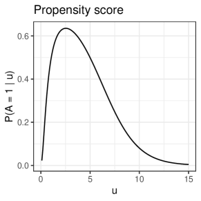
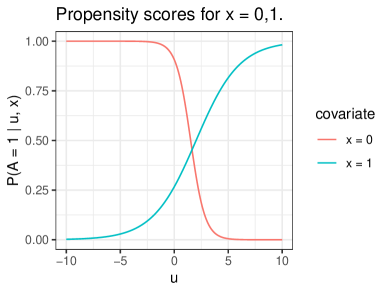
   Figure 3: Left: A plot of the propensity score in setting 6 of Gabriel et al., (2022). Right: A plot of the propensity score in setting 7 of Gabriel et al., (2022) colored by covariate.

Appendix G Examples and counterexamples from Section 6.3

For these set of examples, we consider the case where $U$ and $C$ have 3 levels, and WLOG, we label these $1,2,3$. The $i,j$ entry of a matrix $P_{A\mid B}$ is simply $P(A=i\mid B=j)$, for $i,j\in\{1,2,3\}$.

Example G.1 ($\text{PRD }C\mid U\nRightarrow\text{PRD }U\mid C$).

Consider the following matrix:

$$P_{C\mid U}=\begin{bmatrix}0.4&0.3&0.30\\ 0.5&0.5&0.25\\ 0.1&0.2&0.45\\ \end{bmatrix}.$$

Suppose the marginal distribution of $U$ is given by the probability vector $[0.2,0.5,0.3]^{T}$, where the $j$th entry equals $P(U=j)$. One can check that

$$P_{U\mid C}=\begin{bmatrix}0.25000&0.2352941&0.07843137\\ 0.46875&0.5882353&0.39215686\\ 0.28125&0.1764706&0.52941176\end{bmatrix}.$$

This distribution does not follow PRD, since $P(U\geq 3\mid U=2)=0.1764706<P(U\geq 3\mid U=1)=0.28125$.

Example G.2 ($\text{Tapered }C\mid U\nRightarrow\text{Tapered }U\mid C$).

Consider the following matrix:

$$P_{C\mid U}=\begin{bmatrix}0.39&0.32&0.3\\ 0.31&0.37&0.31\\ 0.3&0.31&0.39\\ \end{bmatrix}.$$

Suppose the marginal distribution of $U$ is given by the probability vector $[0.25,0.4,0.35]^{T}$, where the $j$th entry equals $P(U=j)$. One can check that

$$P_{U\mid C}=\begin{bmatrix}0.2950076&0.2320359&0.2235469\\ 0.3872920&0.4431138&0.3695976\\ 0.3177005&0.3248503&0.4068554\end{bmatrix}.$$

This matrix is not tapered since $P(U=2\mid C=1)=0.3872920>P(U=1\mid C=1)=0.2950076$.

Example G.3 ($C\mid U$ PRD, Tapered, and MLR).

Consider the following matrix:

$$P_{C\mid U}=\begin{bmatrix}0.7&0.25&0.05\\ 0.25&0.5&0.25\\ 0.05&0.25&0.7\end{bmatrix}.$$

This matrix is tapered by inspection. The MLR can be checked by inspecting three sequences: 1) $\frac{P(C=1\mid U=2)}{P(C=1\mid U=1)}=\frac{0.25}{0.7}\leq\frac{P(C=2\mid U=2)}{P(C=2\mid U=1)}=\frac{0.5}{0.25}\leq\frac{P(C=3\mid U=2)}{P(C=3\mid U=1)}=\frac{0.25}{0.05}$, 2) $\frac{P(C=1\mid U=3)}{P(C=1\mid U=1)}=\frac{0.05}{0.7}\leq\frac{P(C=2\mid U=3)}{P(C=2\mid U=1)}=\frac{0.25}{0.25}\leq\frac{P(C=3\mid U=3)}{P(C=3\mid U=1)}=\frac{0.7}{0.05}$, 3) $\frac{P(C=1\mid U=3)}{P(C=1\mid U=2)}=\frac{0.05}{0.25}\leq\frac{P(C=2\mid U=3)}{P(C=2\mid U=2)}=\frac{0.25}{0.5}\leq\frac{P(C=3\mid U=3)}{P(C=3\mid U=2)}=\frac{0.7}{0.25}$.

Example G.4 ($C\mid U$ PRD, not Tapered, and not MLR).

$$P_{C\mid U}=\begin{bmatrix}1/4&1/6&1/7\\ 1/4&1/3&1/7\\ 1/2&1/2&5/7\end{bmatrix}.$$

This is PRD since $P(C\geq 2\mid U=1)=1/4+1/2\leq P(C\geq 2\mid U=2)=1/3+1/2\leq P(C\geq 2\mid U=3)=1/7+5/7$ and $P(C\geq 3\mid U=1)=1/2\leq P(C\geq 3\mid U=2)=1/2\leq P(C\geq 3\mid U=3)=6/7$. This matrix is not MLR since $P(C=2\mid U=3)/P(C=2\mid U=2)=\frac{1/7}{1/3}<P(C=1\mid U=3)/P(C=1\mid U=2)=\frac{1/7}{1/6}$. This matrix is not tapered since $P(C=3\mid U=1)=1/2>P(C=1\mid U=1)=1/4$.

Example G.5 ($C\mid U$ PRD and Tapered, not MLR).

Consider the following matrix:

$$P_{C\mid U}=\begin{bmatrix}0.5&0.25&0.25\\ 0.25&0.5&0.25\\ 0.25&0.25&0.5\end{bmatrix}.$$

It is easy to see that this matrix is tapered. This matrix is not MLR since $P(C=2\mid U=3)/P(C=2\mid U=2)=\frac{0.25}{0.5}<P(C=1\mid U=3)/P(C=1\mid U=2)=\frac{0.25}{0.25}$.

Example G.6 ($C\mid U$ PRD and MLR, not Tapered).

Consider the following matrix:

$$P_{C\mid U}=\begin{bmatrix}1/6&1/6&1/6\\ 1/3&1/3&1/3\\ 1/2&1/2&1/2\end{bmatrix}.$$

This matrix is not tapered since $P(C=3\mid U=1)=1/2>P(C=1\mid U=1)=1/6$. $C$ is independent of $U$, so it trivially follows that the matrix is MLR and PRD.

A more interesting example is the following:

$$P_{C\mid U}=\begin{bmatrix}1/3&0&0\\ 1/6&1/4&1/4\\ 1/2&3/4&3/4\end{bmatrix}.$$

This matrix is not tapered since $P(C=3\mid U=1)=1/2>P(C=1\mid U=1)=1/3$. The MLR can be checked by inspecting three sequences: 1) $\frac{P(C=1\mid U=2)}{P(C=1\mid U=1)}=\frac{0}{1/3}\leq\frac{P(C=2\mid U=2)}{P(C=2\mid U=1)}=\frac{1/4}{1/6}\leq\frac{P(C=3\mid U=2)}{P(C=3\mid U=1)}=\frac{3/4}{1/2}$, 2) $\frac{P(C=1\mid U=3)}{P(C=1\mid U=1)}=\frac{0}{1/3}\leq\frac{P(C=2\mid U=3)}{P(C=2\mid U=1)}=\frac{1/4}{1/6}\leq\frac{P(C=3\mid U=3)}{P(C=3\mid U=1)}=\frac{3/4}{1/2}$, 3) $\frac{P(C=1\mid U=3)}{P(C=1\mid U=2)}=\frac{0}{0}\mathrel{\mathop{\mathchar 58\relax}}=1\leq\frac{P(C=2\mid U=3)}{P(C=2\mid U=2)}=\frac{1/4}{1/4}\leq\frac{P(C=3\mid U=3)}{P(C=3\mid U=2)}=\frac{3/4}{3/4}$.

Appendix H Effect of Treatment on the Treated

As discussed in the main manuscript, the attenuation continues to hold for the effect of the treatment on the treated, i.e. $E[Y(1)-Y(0)\mid A=1]$. The unadjusted, adjusted, and true version of $E[Y(1)\mid A=1]$, coincide, so we need only compare the corresponding versions of $E[Y(0)\mid A=1]$. The unadjusted version is $E[Y\mid A=0]$ since we remain in the setting with no measured confounders. The adjusted version is $\int E[Y\mid A=0,C=c]f(c\mid A=1)$. The true $E[Y(0)\mid A=1]$ can be expressed as $\int E[Y\mid A=0,U=u]f(u\mid A=1)$. We now present two analogous lemmas to 4 and 5. The arguments we present below would need to be slightly altered with measured confounders, and the steps are slightly more involved than incorporating measured confounders for the average treatment effect case; see Theorem 2 of Chiba, (2009).

Lemma H.4.

Under assumptions 1, the positive sign versions of 2, and 3,

$$\int E[Y\mid A=0,C=c]f(c\mid A=1)dc\leq\int E[Y\mid A=0,U=u]f(u\mid A=1)du$$

Proof.

This proof is nearly identical to that of Theorem 2 from Chiba, (2009).

$$\int E[Y\mid A=0,c]f(c\mid A=1)dc=\int\int E[Y\mid A=0,c,u]f(u\mid A=0,c)duf(c\mid A=1)dc$$

$$=\int\int E[Y\mid A=0,c,u]\frac{P(A=0\mid u,c)f(u\mid c)}{P(A=0\mid c)}duf(c\mid A=1)dc$$

$$=\int E_{U\mid c}[E[Y\mid A=0,c,U]P(A=0\mid U,c)]f(c\mid A=1)/P(A=0\mid c)dc$$

$$\leq\int E_{U\mid c}[E[Y\mid A=0,c,U]]E_{U\mid c}[P(A=0\mid U,c)]f(c\mid A=1)/P(A=0\mid c)dc$$

$$=\int E_{U\mid c}[E[Y\mid A=0,c,U]]f(c\mid A=1)dc$$

$$=\int E_{U\mid c}[E[Y\mid A=0,c,U]]E_{U\mid c}[P(A=1\mid U,c)]f(c\mid A=1)/P(A=1\mid c)dc$$

$$\leq\int E_{U\mid c}[E[Y\mid A=0,c,U]P(A=1\mid U,c)]f(c\mid A=1)/P(A=1\mid c)dc$$

$$=\int\int E[Y\mid A=0,c,u]P(A=1\mid u,c)]f(u\mid c)f(c\mid A=1)/P(A=1\mid c)dc$$

$$=\int\int E[Y\mid A=0,c,u]P(A=1\mid u,c)f(u\mid c)f(c)/P(A=1)dudc$$

$$=\int\int E[Y\mid A=0,u]P(A=1\mid u)f(u,c)/P(A=1)dcdu$$

$$=\int\int E[Y\mid A=0,u]P(A=1\mid u)f(c\mid u)f(u)/P(A=1)dcdu$$

$$=\int E[Y\mid A=0,u]P(A=1\mid u)f(u)/P(A=1)du$$

$$=\int E[Y\mid A=0,u]f(u\mid A=1)du.$$

∎

The first inequality is due to $E[Y\mid A=0,C=c,U=u]=E[Y\mid A=0,U=u]$ being non-decreasing in $u$ and $P(A=0\mid C=c,U=u)=P(A=0\mid U=u)$ being non-increasing in $c$ and Lemma 3. The second inequality is also due to Lemma 3 as well as $E[Y\mid A=0,C=c,U=u]=E[Y\mid A=0,U=u]$ and $P(A=0\mid C=c,U=u)=P(A=0\mid U=u)$ both being non-decreasing in $u$. The fourth from the last equality is by Assumption 3.

Lemma H.5.

Under the positive sign versions of assumptions 2, 4, and 3,

$$E[Y\mid A=0]\leq\int E[Y\mid A=0,C=c]f(c\mid A=1)dc$$

Proof.

$$E[Y\mid A=0] =\int E[Y\mid C=c,A=0]f(C=c\mid A=0)dc$$

$$=\int E[Y\mid C=c,A=0]\frac{P(A=0\mid C=c)}{P(A=0)}f(c)dc$$

$$\leq E_{C}[E[Y\mid C,A=0]]\times E_{C}[\frac{P(A=0\mid C=c)}{P(A=0)}]$$

$$=E_{C}[E[Y\mid C,A=0]]$$

$$=E_{C}[E[Y\mid C,A=0]]E_{C}[\frac{P(A=1\mid C=c)}{P(A=1)}]$$

$$\leq\int E[Y\mid C=c,A=0]\frac{P(A=1\mid C=c)}{P(A=1)}f(c)dc$$

$$=\int E[Y\mid C=c,A=0]f(c\mid A=1)dc.$$

The first inequality is due to $E[Y\mid C=c,A=0]$ being non-decreasing in $c$ and $P(A=0\mid C=c)$ being non-increasing in $c$ by Lemma 2 and Lemma 3. The second inequality is also due to Lemma 3 as well as $E[Y\mid C=c,A=0]$ and $P(A=1\mid C=c)$ both being non-decreasing in $c$. ∎

These lemmas together establish that $E[Y\mid A=0]\leq\int E[Y\mid A=0,C=c]f(c\mid A=1)dc\leq\int E[Y\mid A=0,U=u]f(u\mid A=1)du$, establishing the attenuation result for the effect on the treated. An analogous proof can be shown for the effect on the control, which is omitted.

References

• Benjamini and Yekutieli, (2001) Benjamini, Y. and Yekutieli, D. (2001). The control of the false discovery rate in multiple testing under dependency. The Annals of Statistics, 29(4).
• Borges and Pfanzagl, (1963) Borges, R. and Pfanzagl, J. (1963). A characterization of the one parameter exponential family of distributions by monotonicity of likelihood ratios. Zeitschrift fur Wahrscheinlichkeitstheorie und Verwandte Gebiete, 2(2):111–117.
• Chen et al., (2023) Chen, K., Wang, B., and Small, D. S. (2023). A Differential Effect Approach to Partial Identification of Treatment Effects.
• Chiba, (2009) Chiba, Y. (2009). The Sign of the Unmeasured Confounding Bias under Various Standard Populations. Biometrical Journal, 51(4):670–676.
• Ding et al., (2017) Ding, P., Vanderweele, T., and Robins, J. M. (2017). Instrumental variables as bias amplifiers with general outcome and confounding. Biometrika, 104(2):291–302.
• Dwork and Roth, (2013) Dwork, C. and Roth, A. (2013). The algorithmic foundations of differential privacy. Foundations and Trends in Theoretical Computer Science, 9(3-4):211–487.
• Efron, (1965) Efron, B. (1965). Increasing Properties of Polya Frequency Function. The Annals of Mathematical Statistics, 36(1):272–279.
• Esary et al., (1967) Esary, J. D., Proschan, F., and Walkup, D. W. (1967). Association of Random Variables, with Applications. The Annals of Mathematical Statistics, 38(5):1466–1474.
• Gabriel et al., (2022) Gabriel, E. E., Peña, J. M., and Sjölander, A. (2022). Bias attenuation results for dichotomization of a continuous confounder. Journal of Causal Inference, 10(1):515–526.
• Ghassami et al., (2023) Ghassami, A., Shpitser, I., and Tchetgen, E. T. (2023). Partial Identification of Causal Effects Using Proxy Variables.
• Greenland, (1980) Greenland, S. (1980). The Effect of Misclassification in the Presence of Covariates. American Journal of Epidemiology, 112(4):564–569.
• Karlin and Rubin, (1956) Karlin, S. and Rubin, H. (1956). Distributions Possessing a Monotone Likelihood Ratio. Journal of the American Statistical Association, 51(276):637.
• Kuroki and Pearl, (2014) Kuroki, M. and Pearl, J. (2014). Measurement bias and effect restoration in causal inference. Biometrika, 101(2):423–437.
• Lehmann, (1966) Lehmann, E. L. (1966). Some Concepts of Dependence. The Annals of Mathematical Statistics, 37(5):1137–1153.
• Lehmann and Romano, (2022) Lehmann, E. L. and Romano, J. P. (2022). Testing Statistical Hypotheses Fourth Edition.
• Lipsitch et al., (2010) Lipsitch, M., Tchetgen Tchetgen, E., and Cohen, T. (2010). Negative controls: a tool for detecting confounding and bias in observational studies. Epidemiology, 21(3):383–388.
• Miao et al., (2018) Miao, W., Geng, Z., and Tchetgen Tchetgen, E. J. (2018). Identifying causal effects with proxy variables of an unmeasured confounder. Biometrika, 105(4):987–993.
• Ogburn and VanderWeele, (2012) Ogburn, E. L. and VanderWeele, T. J. (2012). On the Nondifferential Misclassification of a Binary Confounder. Epidemiology, 23(3):433–439.
• Ogburn and Vanderweele, (2013) Ogburn, E. L. and Vanderweele, T. J. (2013). Bias attenuation results for nondifferentially mismeasured ordinal and coarsened confounders. Biometrika, 100(1):241–248.
• Park et al., (2024) Park, C., Richardson, D. B., and Tchetgen Tchetgen, E. J. (2024). Single proxy control. Biometrics, 80(2).
• Pearl, (2009) Pearl, J. (2009). Causality. Cambridge University Press.
• Peña, (2020) Peña, J. M. (2020). On the Monotonicity of a Nondifferentially Mismeasured Binary Confounder. Journal of Causal Inference, 8(1):150–163.
• Peña et al., (2021) Peña, J. M., Balgi, S., Sjölander, A., and Gabriel, E. E. (2021). On the bias of adjusting for a non-differentially mismeasured discrete confounder. Journal of Causal Inference, 9(1):229–249.
• Rosenbaum, (1989) Rosenbaum, P. R. (1989). The Role of Known Effects in Observational Studies. Biometrics, 45(2):557.
• Rosenbaum, (2006) Rosenbaum, P. R. (2006). Differential effects and generic biases in observational studies. Biometrika, 93(3):573–586.
• Sjölander et al., (2022) Sjölander, A., Peña, J. M., and Gabriel, E. E. (2022). Bias results for nondifferential mismeasurement of a binary confounder. Statistics & Probability Letters, 186:109474.
• Tchetgen Tchetgen, (2014) Tchetgen Tchetgen, E. (2014). The Control Outcome Calibration Approach for Causal Inference With Unobserved Confounding. American Journal of Epidemiology, 179(5):633–640.
• VanderWeele, (2008) VanderWeele, T. J. (2008). The Sign of the Bias of Unmeasured Confounding. Biometrics, 64(3):702–706.
• Wang and Gustafson, (2014) Wang, D. and Gustafson, P. (2014). On the Impact of Misclassification in an Ordinal Exposure Variable. Epidemiologic Methods, 3(1).