Conformity assessment of processes and lots in the framework of JCGM 106:2012

Abstract

ISO/IEC 17000:2020 defines conformity assessment as an "activity to determine whether specified requirements relating to a product, process, system, person or body are fulfilled". JCGM (2012) establishes a framework for accounting for measurement uncertainty in conformity assessment. The focus of JCGM (2012) is on the conformity assessment of individual units of product based on measurements on a cardinal continuous scale. However, the scheme can also be applied to composite assessment targets like finite lots of product or manufacturing processes, and to the evaluation of characteristics in discrete cardinal or nominal scales.

We consider the application of the JCGM scheme in the conformity assessment of finite lots or processes of discrete units subject to a dichotomous quality classification as conforming and nonconforming. A lot or process is classified as conforming if the actual proportion nonconforming does not exceed a prescribed upper tolerance limit, otherwise the lot or process is classified as nonconforming. The measurement on the lot or process is a statistical estimation of the proportion nonconforming based on attributes or variables sampling, and meassurement uncertainty is sampling uncertainty. Following JCGM (2012), we analyse the effect of measurement uncertainty (sampling uncertainty) in attributes sampling, and we calculate key conformity assessment parameters, in particular the producer’s and consumer’s risk. We suggest to integrate such parameters as a useful add-on into ISO acceptance sampling standards such as the ISO 2859 series.

1 Introduction

The sampling inspection of discrete units of finished product assembled in lots is often addressed as acceptance sampling. The ISO acceptance sampling standards, in particular the 2859 series for attributes sampling, and 3951 series for variables sampling, provide a comprehensive and structured normative framework which is accepted and used worldwide transversally in different industrial sectors. Our study focusses on attributes sampling. Suitably adapted, the same approach can be used for variables sampling.

Sampling inspection of finished product on a regular mass basis has been disappearing from industry over the past decades. Nevertheless acceptance sampling inspection continues to be used as a tool of quality control in many industrial contexts (Gravesetal(2000) (1), Derosetal(2008) (2)), in particular in specific industrial sectors as the pharmaceutical, medical devices, and food industries, where the use of sampling policies is imposed by regulatory authorities. Schilling(2017) (3) lists ten reasons for the use of acceptance sampling in modern quality assurance.

The ISO 2859 attributes sampling series evolved from the US Military Standard MIL-STD-105. MIL-STD-105A (MILSTD105A (4)) arose in 1950 as a compromise between sampling schemes developed for the US Army and US Navy during World War II (Dodge(1969a) (4), Dodge(1969b) (5), Dodge(1969c) (6), Dodge(1969d) (7), Schilling(2017) (3)). Updated versions were issued as MIL-STD-105B (MILSTD105B (5), 1958), MIL-STD-105C (MILSTD105C (6), 1961), MIL-STD-105D (MILSTD105D (7), 1963), and finally MIL-STD-105E (MILSTD105E (8), 1989). The first ISO attributes sampling standard was issued in 1974 as ISO 2859, with minor changes adopted from MIL-STD-105D. In the 1980s, ISO 2859 was integrated into the ISO 2859 attributes sampling series which currently has two major complementary parts: ISO 2859-1 ISO2859-1 (9), widely identical with MIL-STD-105E (Balaetal(2008) (1)), targets a continuing series of lots from an identifiable process, whereas ISO 2859-2 ISO2859-2 (10) is designed for the inspection of isolated lots (GoebandBaillie(2012) (2)).

The revisions leading from MIL-STD-105A to MIL-STD-105E and finally to ISO 2859-1 were mainly on wording, arrangement of content, and some enlargement of the range of quality parameters. The core concept and the sampling tables remained invariant. The ISO 2859 attributes sampling series widely reflects a view of acceptance sampling shaped in World War II. Two characteristic principles of historic acceptance sampling can be identified (Dodge&Romig(1959) (8), p. 11; Duncan(1974) (9), p. 9): H1) The core purpose of acceptance sampling is the decision on the acceptability of lots submitted for inspection ("sorting good lots from bad", Dodge&Romig(1959) (8)), but not the provision of information on the actual lot or process quality. H2) Acceptance sampling is a stand-alone tool without organised embedding in a system of quality assurance and without an organised flow of information to and from other quality assurance system components.

Both principles H1) and H2) are contradicting the principles of modern quality control systems where various control functions are assembled in a coordinated system with an organised exchange of information, betweeen all system components. In such a system, acceptance sampling plays rather an adjunct than a central role (Feigenbaum(2004) (10)). Acceptance sampling schemes need to consider prior information on product quality (Godfrey&Mundel(1984) (11)). Beyond decision on acceptability, the provision of information on the actual state of product quality and the operational risks of sampling inspection is a core task of acceptance sampling.

Conformity assessment is an important function of product quality control (Liepinaetal(2014) (12)). Pendrill(2014) (13) defines:

Conformity assessment, broadly defined, is any activity undertaken to determine, directly or indirectly, whether an entity (product, process, system, person or body) meets relevant standards or fulfils specified requirements.

JCGM 106:2012 (JCGM(2012) (14)), issued by the Joint Committee on Guides in Metrology (JCGM), is a guidance document for conformity assessment under uncertain measurements of the target entity’s relevant characteristics. The underlying Bayesian scheme accounts for prior information on the target characteristics, and allows to calculate informative indicators, in particular conformance probabilities and risk measures.

JCGM 106:2012 focusses the conformity assessment of individual units (items) of product. We adapt the scheme for the conformity assessment of finite lots or continuous processes of discrete units under the quality model of attributes sampling. I. e., the items are subject to a dichotomous quality classification “conforming” versus “nonconforming”, and the quality of the lot or process is expressed by the proportion nonconforming. A lot or process is classified as conforming if the actual proportion nonconforming does not exceed a prescribed upper tolerance limit, otherwise the lot or process is classified as nonconforming. The measurement on the lot or process is a statistical estimation of the proportion nonconforming, and meassurement uncertainty is sampling uncertainty.

We suggest to supplement ISO acceptance sampling standards by procedures of conformity assessment of lots and processes according to JCGM 106:2012. This will enable the standards to correspond to essential requirements of contemporary quality control by processing prior knowledge on lot or process quality, and by providing informative conformity indicators.

The present study uses attributes sampling as a paradigm for outlining the adaptation of the JCGM 106:2012 scheme to acceptance sampling. Suitably modified, the approach can also be used fpr sampling by variables. The study is organised in the following sections:

2 Basics of the JCGM 106:2012 conformity assessment scheme

The conformity requirements relative to some target entity are expressed by a tolerance region (conformance region) ${\cal C}$ imposed on the level $X$ of a scalar measurable characteristic of the target entity. $X$ is addressed as the target variable. The entity fulfills the requirements and is conforming if $X\in{\cal C}$, otherwise the entity is nonconforming. Conformity assesment proceeds by comparing a measurement $Y$ of the unknown measurand $X$ with an acceptance region $\cal A$: the target entity is assessed as conforming (acceptance) if $Y\in{\cal A}$, otherwise the target entity is assessed as nonconforming (rejection). In standard applications, both the conformance region ${\cal C}$ and the accceptance region ${\cal A}$ are one-sided or two-sided intervals. See table 1 for a survey of the basic conformity assessment concepts.

JCGM 106:2012 is a Bayesian analysis scheme and accounts for prior knowledge. The pre-measurement knowledge on the measurand $X$ is conveyed by the unconditional prior PDF $f_{X}$ of $X$. The relation between the measurement $Y$ and the measurand $X$ is uncertain, $Y$ is potentially deviating from the measurand $X$. The post-measurement knowledge conveyed by $Y$ on the measurand $X$ is expressed by the posterior conditional PDF $f_{X|Y=y}$. The joint unconditional PDF $f_{X,Y}$, the unconditional PDFs $f_{X}$ and $f_{Y}$, and the pre-measurement and post-measurement PDFs are related by Bayes’ theorem as

$$\begin{array}[]{l}\displaystyle f_{X|Y=y}(x)\;\;=\;\;f_{Y|X=x}(y){f_{X}(x)\over f_{Y}(y)}\;\;=\;\;{f_{X,Y}(x,y)\over f_{Y}(y)}.\end{array}$$ (1)

Table 1: Basic components of the JCGM 106:2012 conformity assessment scheme

$X$	rating variable, i. e., the level of a measurable characteristic used for rating the conformity of the target entity
$Y$	a measurement of the level of the rating characteristic
$\cal C$	tolerance or conformance region, i. e., the set of rating characteristic levels $X=x$ such that the target entity is rated as conforming
$\cal A$	acceptance region of the conformity assessment test, i. e., the set of permissible measurements $Y=y$ under which the target entity is assessed as conforming

JCGM 106:2012 focusses on the continuous case where all PDFs are densities relative to the Lebesgue-Borel measure. In a straightforward manner, the scheme can be generalised to densities relative to an arbitrary dominating measure $\nu$, in particular a suitable counting measure in the discrete case. To avoid an inflation of symbols, we use $\nu$ as the generic notation for the dominating measure in the sequel.

3 Conformity indicators and risk indicators suggested by the JCGM 106:2012 scheme

Table 2: Erroneous and correct results of binary conformity assessment

	$X\in{\cal C}$	$X\notin{\cal C}$
$Y\in{\cal A}$	correct acceptance	erroneous acceptance
$Y\notin{\cal A}$	erroneous rejection	correct rejection

The suitable indicator for the conformity status of the target entity under a given measurement $Y=y$ is the posterior conformance probability

$$\begin{array}[]{l}\displaystyle p_{{\cal C}|y}\;\;=\;\;\mbox{P}(X\in{\cal C}|Y=y)\;\;=\;\;\int_{y\in{\cal C}}f_{X|Y=y}(y)\,\mbox{d}\nu(y).\end{array}$$ (2)

Erroneous and correct results of the binary conformity assessment procedure are classified by table 2. The operational risks of the conformity assessment procedure are measured by the probabilities of erroneous assessment results, with different focus for the consumer and for the producer.

The consumer suffers from erroneously assessing a nonconforming target entity as conforming. Thus the specific consumer’s risk is the conditional probability

$$\begin{array}[]{l}\displaystyle R^{\star}_{\mbox{\scriptsize Con}|y}\;\;=\;\;\mbox{P}(X\notin{\cal C}|Y=y)\;\;=\;\;1-p_{{\cal C}|y}\quad\mbox{for }y\in{\cal A}.\end{array}$$ (3)

The producer suffers from erroneously assessing a conforming target entity as nonconforming. Thus the specific producer’s risk is the conditional probability

$$\begin{array}[]{l}\displaystyle R^{\star}_{\mbox{\scriptsize Pro}|y}\;\;=\;\;\mbox{P}(X\in{\cal C}|Y=y)\;\;=\;\;p_{{\cal C}|y}\quad\mbox{for }y\notin{\cal A}.\end{array}$$ (4)

The global risks are the unconditional probabilities of unfavourable events either from the consumer’s or from the producer’s point of view. The global consumer’s risk is

$$\begin{array}[]{l}\displaystyle R_{\mbox{\scriptsize Con}}\;\;=\;\;\mbox{P}(X\notin{\cal C},Y\in{\cal A})\;\;=\;\;\int_{x\notin{\cal C},y\in{\cal A}}f_{X,Y}(x,y)\,\mbox{d}\nu(x,y)\;\;=\\[11.38109pt] \displaystyle\int_{y\in{\cal A}}[1-p_{{\cal C}|y}]f_{Y}(y)\,\mbox{d}\nu(y),\end{array}$$ (5)

and the global producer’s risk is

$$\begin{array}[]{l}\displaystyle R_{\mbox{\scriptsize Pro}}\;\;=\;\;\mbox{P}(X\in{\cal C},Y\notin{\cal A})\;\;=\;\;\int_{x\in{\cal C},y\notin{\cal A}}f_{X,Y}(x,y)\,\mbox{d}\nu(x,y)\;\;=\\[8.53581pt] \displaystyle\int_{y\notin{\cal A}}p_{{\cal C}|y}f_{Y}(y)\,\mbox{d}\nu(y).\end{array}$$ (6)

From (5) and (6) we obtain the equation

$$\begin{array}[]{l}\displaystyle R_{\mbox{\scriptsize Con}}\;\;=\;\;\mbox{P}(Y\in{\cal A})-\mbox{P}(X\in{\cal C})+R_{\mbox{\scriptsize Pro}}.\end{array}$$ (7)

4 Statistical product inspection as an instance of the JCGM 106:2012 scheme

We illustrate the use of the JCGM 106:2012 model as a conceptual scheme for statistical product inspection in an exemplary manner by analysing single sampling plans for a proportion nonconforming of a lot or a process. Our approach can easily be adapted to more refined sampling plans and to other quality models, in particular to sampling by variables.

The components of the JCGM 106:2012 conformity assessment scheme as displayed by table 1 are identified as follows. The target entity is a lot or process of discrete units $i$ with associated dichotomous quality indicators $U_{i}\in\{0,1\}$ where $U_{i}=1$ if unit $i$ nonconforming, and $U_{i}=0$ if unit $i$ conforming. If the target entity is the process, the target variable $X$ (rating variable) is the process proportion nonconforming $X=\pi$ where $\mbox{P}(U_{i}=1|\pi=p)=p$. If the target entity is a lot of units $i=1,...,N$, the target variable $X$ (rating variable) is the proportion nonconforming $(U_{1}+...+U_{N})/N$ of the lot, or, equivalently the number $X=U_{1}+...+U_{N}$ of nonconforming units in the lot. Both for the process and for the lot case, the tolerance region is an interval ${\cal C}=[0\mathchar 24635\relax\;x_{\cal C}]$ with the lower tolerance limit 0 and the upper tolerance limit $x_{\cal C}$.

The measurement used for evaluating the unknown lot or process proportion nonconforming $X$ is the number $Y$ of nonconforming units in a random sample of size $n$ from the lot or the process. The acceptance region of acceptance sampling by a single sampling plan $(n,c)$ is ${\cal A}=\{0,...,c\}$ with the acceptance number $c$, i. e., the lot/process is assessed as conforming if $Y\leq c$, and as nonconforming if $Y\geq c+1$.

The probability distributions of the number $Y$ of nonconforming units in a random sample of size $n$ from the lot or the process are analysed in sections 7 and 8, below.

5 Risk concepts of ISO 3534 versus risk concepts of JCGM106:2021

This section analyses the marked contrast between the risk indicators coined by JCGM106:2021, see the above section 3, and the risk indicators defined by the ISO standard ISO 3534-2:2006 (ISO3534-2 (16)). A synopsis of the risk indicators from the two documents is provided by table 3.

In both conceptual frameworks, the specific risk indicators are conditional probabilities where the positions of the conditioning and the conditioned event are permuted between the frameworks. ISO 3534-2:2006 considers the probability of an erroneous result of the conformity assessment procedure based on the measurement $Y$, conditioned under a specific value of the rating characteristic $X$. JCGM106:2021 considers the probability of a result of the conformity rating based on $X$, conditioned under a specific value of the measurement $Y$. The global risks by JCGM106:2021 are the total probabilities of an erroneous conformity assessment from the consumer’s and the producer’s perspective. ISO 3534-2:2006 doesn’t define global risk.

The two risk concepts should be considered as complementary rather than as conflicting. In the statistical product inspection framework established by paragraph 4 we illustrate the complementarity of the risk concepts with respect to two aspects: i) operational usefulness, and ii) usefulness for the design of sampling plans.

Operational usefulness: The specific risk concepts by ISO are operationally useless for product inspection. The value $x$ of the lot or process proportion nonconforming in the conditioning event $X=x$ is unknown at the inspection operation. Hence no inferences can be drawn from probabilities of the type $\mbox{P}(\cdot|X=x)$. On the contrary, the specific risks by JCGM106:2021 are useful for the inspection operation. The value $Y=y$ of the number of nonconforming units in the sample is determined in course of the inspection operation, and can serve for inference on the target rating variable $X$.

Design usefulness: The specific risk concepts by ISO are useful for the design of statistical product inspection. Based on their insights into the respective business processes, the producer and the consumer use to have precise ideas on critical levels $x$ of the proportion nonconconforming. Thus it makes sense to design inspection procedures in a way to restrict the probability of rejection at particularly low levels of the proportion nonconforming, and the probability of acceptance at particularly high levels of the proportion nonconforming by specified bounds, usually 5 % or 10 %, see the standards ISO 2859-1 ISO2859-1 (9) and ISO 2859-2 ISO2859-2 (10). On the contrary, the specific risk concepts by JCGM106:2021 are not useful for the design of product inspection procedure. The number $Y$ of nonconforming units in a sample is not related to any business process characteristics. Thus designing sampling plans based on specific values $Y=y$ makes no sense.

Table 3: Risk concepts in JCGM106:2021 and in ISO 3534-2:2006

guidance document	risk type	consumer’s risk	producer’s risk
	specific	$\mbox{P}(X\notin{\cal C}|Y=y)$,   $y\in{\cal A}$	$\mbox{P}(X\in{\cal C}|Y=y)$,   $y\notin{\cal A}$
JCGM106:2021	global	$\mbox{P}(X\notin{\cal C},Y\in{\cal A})$	$\mbox{P}(X\in{\cal C},Y\notin{\cal A})$
	specific	$\mbox{P}(Y\in{\cal A}|X=x)$ ,   $x\notin{\cal C}$	$\mbox{P}(Y\notin{\cal A}|X=x)$,  $x\in{\cal C}$
ISO 3534-2:2006	global	—	—

6 Prior information modelling

Consider the statistical product inspection framework established by section 4. As stipulated by ISO 2859-1 ISO2859-1 (9), the discrete items $...,i-1,i,i+1,...$ are the outcome of a unique and stable production process. In stochastic terms, the series of dichotomous quality indicators $...,U_{i-1},U_{i},U_{i+1},...$ form an i.i.d. process of Bernoulli variables $U_{i}\sim Bi(1,p)$ in the conditional situation with a given values $\pi=p$ of the process proportion nonconforming. In this framework, prior information modelling means to specify the distribution of the random process proportion nonconforming $X=\pi$. A finite lot of items $1,...,N$ is considered as a segment of the process. Thus a prior for the random process proportion nonconforming $X=\pi$ implicitly determines a prior for the lot proportion nonconforming, see section 8, below.

As a prior for the process proportion nonconforming $X=\pi$ we use a beta distribution $BETA(a,b)$ defined by the PDF

$$\begin{array}[]{l}\displaystyle f_{a,b}(x)\;\;\;=\;\;\;\left\{\begin{array}[]{ll}{x^{a-1}(1-x)^{b-1}\over B(a,b)}&\mbox{ for }\;0<x<1,\\ &\\ 0&\mbox{ otherwise, }\end{array}\right.\end{array}$$ (8)

with parameters $a,b>0$, where

$$\begin{array}[]{l}\displaystyle B(a,b)\;\;\;=\;\;\;{\Gamma(a+b)\over\Gamma(a)\Gamma(b)}\;\;\;=\;\;\;B(b,a)\end{array}$$ (9)

is the symmetric beta function and $\Gamma$ denotes the well-known gamma function.

The beta distribution model has several appealing characteristics: flexibility; sparse parametrisation by only two parameters; the property of being the conjugate prior for the binomial distribution; the potential to express various density shapes like bathtub, inverted bathtub, strictly decreasing, strictly increasing, constant (equidistribution). Thus the beta distribution has become the preferred distribution for expressing prior information on random quantities ranging over compact intervals, in particular proportions and probabilities, in various areas of interest, e. g., interval estimation (GoebLurz (18)), acceptance sampling (Hald (19)), audit sampling (Godfrey&Andrews(1982) (20), Berg(2006) (21)), risk analysis (Kendrick(2009) (22)), forecasting (Kim&Reinschmid(2009) (23)), analysis of measurement error (Eschmannetal(2019) (24)).

In industrial and business environments, the assignment of values to the beta parameters $a$ and $b$ may not be based on subjective reasoning in the sense of arbitrary and methodically not defensible conjectures. In the case of repetitive sampling from a process with proportion nonconforming $\pi$, the parameters of the prior information distribution can be estimated from accumulated historical sample data. If sufficient sound and reliable reference data are not available, the features of the distribution have to be elicited from expert opinions in interviews or panels. The process of eliciting distprributions from experts has received considerable interest in the literature, with particular emphasis on the beta distribution, see Corless(1972) (25), Hogarth(1975) (26), Kadaneetal(1980) (27) Chaloner&Duncan(1983) (28), O'Hagan(1998) (29), Walls&Quigley(2001) (30). Software assisted approaches are considered by Blocher&Robertson(1976) (31) or Garthwaite&O'Hagan(2000) (32).

A simple algorithm for determining the beta parameters has the following steps: i) Specify the support $[p_{0}\mathchar 24635\relax\;p_{1}]$ of $Y$. ii) Specify the mean $\mu_{Y}$. iii) Specify a quantile $p_{\rho}$, i. e., a value $p_{\rho}$ with $F_{Y}(p_{\rho})=\rho$. iv) Solve for the parameters $a$ and $b$. In modern industrial and business environments very small values $\pi=p$ are to be expected. For this case, an appropriate model is a prior density $f_{a,b}$ decreasing on $[0\mathchar 24635\relax\;1]$ with a large probability mass close to 0. A simple instance of this shape is a beta distribution $B(1.0,b)$ with first parameter $a=1.0$. Then the second parameter $b$ is uniquely determined by specifying either the mean $\mu_{Y}$ or a quantile $p_{\rho}$.

7 Analysing process conformance

Consider a process $...,i-1,i,i+1,...$ of discrete units $i$ with the dichotomous quality indicator $U_{\ell}$ where $U_{\ell}=1$ if unit $\ell$ nonconforming, $U_{\ell}=0$ if unit $i$ conforming. The target entity is the process $(U_{i})$, and the target characteristic is the random process proportion nonconforming $X=\pi$. The tolerance region is an interval ${\cal C}=[0\mathchar 24635\relax\;x_{\cal C}]$ with the lower tolerance limit 0 and the upper tolerance limit $x_{\cal C}$. The target characteristic (process proportion nonconforming) is evaluated by the number $Y$ of nonconforming units in a random sample from the process. The acceptance region is ${\cal A}=\{0,...,c\}$ with the acceptance number $c$, i. e., the process is assessed as conforming if $Y\leq c$, and as nonconforming if $Y\geq c+1$.

In the process, the quality indicators $U_{i}$ are assumed to be independent Bernoulli variables, i. e., conditional on a value $\pi=p$ of the process proportion nonconforming $\pi$, each item quality indicator $U_{i}$ is distributed by the binomial distribution $Bi(1,p)$. Hence, conditional on $\pi=p$, the number $Y$ of nonconforming units in a random sample of size $n$ from the process is distributed by the binomial distribution $Bi(n,p)$.

Under the prior information model established by section 6, the random process proporion nonconforming $X=\pi$ is assumed to be distributed by a beta distribution $BETA(a,b)$. Hence by assertion b) of proposition 1 in the appendix A, the unconditional distribution of the number $Y$ of nonconforming units in the sample is the univariate beta-binomial distribution $BETA$-$Bi(n,a,b)$ with PDF provided by equations (19) and (20).

By assertion c) of proposition 1 the posterior conditional distribution of the process proportion nonconforming $X=\pi$ under a given number $Y=y$ is the beta distribution $BETA(a+y,b+n-y)$ for $y\in\{0,...,n\}$. Using the Lebesgue measure $\nu$ as in the equations provided by section 3, the conformity indicators and risk indicators can be expressed with the CDF $F_{\mbox{\scriptsize$BETA(a+y,b+n-y)$}}$ of the beta distribution $BETA(a+y,b+n-y)$. The conditional conformance probability is obtained from equation (2) as

$$\begin{array}[]{l}\displaystyle p_{{\cal C}|y}\;\;=\;\;\mbox{P}(X\leq x_{\cal C}|Y=y)\;\;=\;\;F_{\mbox{\scriptsize$BETA(a+y,b+n-y)$}}(x_{\cal C}).\end{array}$$ (10)

By the equations (3) and (4) the specific consumer’s risk and the specific producer’s risk are

$$\begin{array}[]{l}\displaystyle R^{\star}_{\mbox{\scriptsize Con}|y}\;\;=\;\;\mbox{P}(X\notin{\cal C}|Y=y)\;\;=\\[8.53581pt] \displaystyle 1-F_{\mbox{\scriptsize$BETA(a+y,b+n-y)$}}(x_{\cal C})\quad\mbox{for }\;y\leq c,\end{array}$$ (11)

$$\begin{array}[]{l}\displaystyle R^{\star}_{\mbox{\scriptsize Pro}|y}\;\;=\;\;\mbox{P}(X\in{\cal C}|Y=y)\;\;=\\[8.53581pt] \displaystyle F_{\mbox{\scriptsize$BETA(a+y,b+n-y)$}}(x_{\cal C})\quad\mbox{for }\;y\geq c+1.\end{array}$$ (12)

Using (5), we obtain the global consumer’s risk

$$\begin{array}[]{l}\displaystyle R_{\mbox{\scriptsize Con}}\;\;=\\[8.53581pt] \displaystyle\sum_{y\leq c}{n\choose y}{B(a+y,b+n-y)\over B(a,b)}[1-F_{\mbox{\scriptsize$BETA(a+y,b+n-y)$}}(x_{\cal C})].\\[8.53581pt] \displaystyle\end{array}$$ (13)

8 Analysing lot conformance

Consider discrete units $i$ with the dichotomous quality indicator $U_{i}$ where $U_{i}=1$ if unit $i$ nonconforming, $U_{i}=0$ if unit $i$ conforming. The item quality indicators $U_{1},...,U_{N}$ are considered as a segment of an i.i.d. process where $U_{i}\sim Bi(1,p)$ with the process proportion nonconforming $\pi=p$.

The target entity is a lot $1,...,N$ of size $N$ composed of such units with associated quality indicators $U_{1},...,U_{N}$. The target characteristic is the number $X=U_{1}+....+U_{N}$ of nonconforming units in the lot, or, equivalently, the lot proportion nonconforming $X/N$. The tolerance region is an interval ${\cal C}=[0\mathchar 24635\relax\;x_{\cal C}]$ with the lower tolerance limit 0 and the upper tolerance limit $x_{\cal C}$. The target characteristic is evaluated by the number $Y$ of nonconforming units in a random sample of size $n$ from the lot. The acceptance region is ${\cal A}=\{0,...,c\}$ with the acceptance number $c$, i. e., the process is assessed as conforming if $Y\leq c$, and as nonconforming if $Y\geq c+1$.

Conditional on a value $\pi=p$ of the process proportion nonconforming, we have $X\sim Bi(N,p)$, $Y\sim Bi(n,p)$, $X-Y\sim Bi(N-n,p)$, where $Y$ and $X-Y$ are independent. Under the prior information model established by section 6, the random process proporion nonconforming $\pi$ is assumed to be distributed by a beta distribution $BETA(a,b)$. Hence inserting $Z_{1}=Y$,$n_{1}=n$, $Z_{2}=X-Y$, $n_{2}=N-n$ in the assertion c) of proposition 1 in the appendix A we obtain for $y=0,...,n$, $x=y,...,N-n$

$$\begin{array}[]{l}\displaystyle f_{X|Y=y}(x)\;\;=\;\;\mbox{P}(X-Y=x-y|Y=y)\;\;=\\[17.07164pt] \displaystyle{N-n\choose x-y}{B(a+x,b+N-x)\over B(a+y,b+n-y)}\;\;=\;\;f_{N-n,a+y,b+n-y}(x-y)\end{array}$$ (14)

where the PDF $f_{N-n,a+y,b+n-y}$ of the beta-binomial distribution $BETA$-$Bi(N-n,a+y,b+n-y)$ is defined by equation (19). By assertion b) of proposition 1 in the appendix A the unconditional distrinution of the number $Y$ of nonconforming units in the sample is the beta-binomial distribution $BETA$-$Bi(n,a,b)$.

Using the Lebesgue measure $\nu$ as in the equations provided by section 3, the conformity indicators and risk indicators can be expressed with the CDF $F_{\mbox{\scriptsize$BETA$-$Bi(N-n,a+y,b+n-y)$}}$ of the beta-binomial distribution $BETA$-$Bi(N-n,a+y,b+n-y)$. The conditional conformance probability is obtained from equation (2) as

$$\begin{array}[]{l}\displaystyle p_{{\cal C}|y}\;\;=\;\;\mbox{P}(X\leq x_{\cal C}|Y=y)\;\;=\;\;F_{\mbox{\scriptsize$BETA-Bi(N-n,a+y,b+n-y)$}}(x_{\cal C}-y).\end{array}$$ (15)

By the equations (3) and (4) the specific consumer’s risk and the specific producer’s risk are

$$\begin{array}[]{l}\displaystyle R^{\star}_{\mbox{\scriptsize Con}|y}\;\;=\;\;\mbox{P}(X\notin{\cal C}|Y=y)\;\;=\\[8.53581pt] \displaystyle 1-F_{\mbox{\scriptsize$BETA$-$Bi(N-n,a+y,b+n-y)$}}(x_{\cal C}-y)\quad\mbox{for }\;y\leq c,\end{array}$$ (16)

$$\begin{array}[]{l}\displaystyle R^{\star}_{\mbox{\scriptsize Pro}|y}\;\;=\;\;\mbox{P}(X\in{\cal C}|Y=y)\;\;=\\[8.53581pt] \displaystyle F_{\mbox{\scriptsize$BETA-Bi(N-n,a+y,b+n-y)$}}(x_{\cal C}-y)\quad\mbox{for }\;y\geq c+1.\end{array}$$ (17)

Using (5), we obtain the global consumer’s risk

$$\begin{array}[]{l}\displaystyle R_{\mbox{\scriptsize Con}}\;\;=\\[8.53581pt] \displaystyle\sum_{y\leq c}{n\choose y}{B(a+y,b+n-y)\over B(a,b)}[1-F_{\mbox{\scriptsize$BETA-Bi(N-n,a+y,b+n-y)$}}(x_{\cal C})-y].\\[8.53581pt] \displaystyle\end{array}$$ (18)

9 Numerical results on lot conformance indicators

The consumer’s direct concern is the respective lot of product under consideration. The process is relevant for long-term considerations whereas the state of the lot direct affectly affects the consumer’s technical and business process. Hence it is most interesting to consider the conformance indicators generally defined by section 3 for the case of lot evaluation, using the analytical results of section 8.

For inspecting for a proportion of nonconforming items, ISO 2859-1 ISO2859-1 (9) is the most common sampling standard in industry. The standard targets the process behind the stream of lots. However, in business practice the consumer needs to take decisions on each individual lot submitted for inspection. So the indvidual lot is the primary target for conformity assessment.

We consider the sampling plans from ISO 2859-1 in the most widely used categories: normal inspection, general inspection level II. ISO 2859-1 indexes the sampling plans in the lot size $N$ and in the AQL (acceptance quality limit) which is defined as the “worst tolerable quality level” (ISO 3534-2:2006 ISO3534-2 (16)), here the worst tolerable level of the proportion nonconforming. As such, the AQL is the natural choice for the upper bound of the tolerance or conformance region $\cal C$, see table 1. ISO 2859-1 lists 26 AQL percentages in approximate geometric progression $0.01\times 10^{i/5}$, $i=0,...,25$. The 7 largest values are inadequate for a percentage nonconforming, and do only make sense for quality statements in the case of nonconformities per 100 items. For our numerical experiments we consider the lot size $N=1200$. So we restrict attention to the 19 AQL values and the corresponding single sampling plans from ISO 2859-1 under lot size $N=1200$ for normal inspection, general inspection level II, listed by table 4.

So as to adapt the AQL to the lot quality scheme exposed by section 4 we have to round the AQL to a value which can appear as a fraction $X/N$ for some number $X$ of nonconforming units under a given lot size $N$. In agreement with the definition as the “worst tolerable quality level” we use the value $x_{\cal C}=\lfloor\mbox{AQL}/100\times N\rfloor$ as the upper bound for the tolerance or conformance region for the number $X$ of nonconforming units in the lot.

Prior information is expressed by a beta distribution of the process proportion nonconforming, see section 6. We evaluate the effect of prior information by considering the beta distributions $BETA(a,b)$ with the parameter pairs $(a,b)$ listed by table 5. As visible from the respective means and 99 % quantiles the parameter pairs cover cover a broad range of states of the process proportion nonconforming. In the light of the quality levels usually required in modern industrial and business environments all considered distributions amount to relatively conservative assumptions. Even the most restrictive assumption with $a=0.24$ and $b=78.12$, mean 0.003 (3 permil nonconorming units on average) and 99 % quantile $z_{a,b}(0.99)=0.030$ (percentage of nonconforming units not exceeding 3 percent in 99 % of all cases) is not unrealistically optimistic in a modern industrial environment. The beta distribution with $(a,b)=(1,1)$ amounts to equidistribution of the proportion nonconforming over the unit interval, i. e., no specific prior information.

The figures 1 and 2 provide the lot conformance probability $p_{{\cal C}|0}$ under $x_{\mbox{\scriptsize ev}}=0$ observed nonconforming units in a sample from a lot of size $N=1200$. Figure 1 compares the effect of the two extreme priors $(a,b)=(1,1)$ (no prior information) and $(a,b)=(0.24,78.12)$, under the 19 AQLs from table 4. Without specific prior information, the conformance probability is particularly small under the sample sizes corresponding to moderate AQLs. For the latter, specific prior information is able to leverage the conformance probability to moderate up to high values. Figure 2 illustrates the leveraging effect of prior information along the nine pairs $(a,b)$ from table 5 under the specific choice $\mbox{AQL}=0.04$ in percent which amounts to a sample size $n=315$.

The figures 3 and 4 consider the specific risk indicators introduced in section 3: i) the specific consumer’s risk defined by formula (3) as the conditional probability of finding an actually nonconforming lot with $X>x_{\cal C}$ conditional on a sample result which enforces assessment of the lot as conforming; ii) the specific producer’s risk defined by formula (4) as the conditional probability of finding an actually conforming lot conditional on a sample result which enforces assessment of the lot as nonconforming.

By the model of section 4, under a single sampling plan $(n,c)$ sample results $0\leq Y\leq c$ (number $Y$ of nonconforming units in sample not exceeding the acceptance number $c$) lead to assessing the lot as conforming, and sample results $Y\geq c+1$ (number $Y$ of nonconforming units in sample exceeding the acceptance number $c$) lead to assessing the lot as nonconforming. In the figures 3 and 4 we consider sample results at the margin of the acceptance region: $Y=c$ as the condition for the consumer’s risk $R^{\star}_{\mbox{\scriptsize Con}|Y=c}=\mbox{P}(X>x_{\cal C}|Y=c)$, and $Y=c+1$ as the condition for the producer’s risk $R^{\star}_{\mbox{\scriptsize Pro}|Y=c+1}=\mbox{P}(X\leq x_{\cal C}|Y=c+1)$. Figure 3 considers the beta prior with $(a,b)=(1,1)$ (no prior information), whereas figure 4 considers the most restrictive prior with $(a,b)=(0.24,78.12)$. The calculations range over the 19 AQLs with corresponding conformance limit $x_{\cal C}$ and single sampling plans $(n,c)$ listed by table 4.

The figures 3 and 4 show that under both priors, the producer’s risk is low and the consumer’s risk is high. Particularly under the small sample sizes recommended by ISO 2859-1 for large AQL, the consumer’s risk is close to 1. In the considered situation of $Y=c$ nonconforming units in the sample, so that the lot is marginally accepted, it is practically certain that the consumer will erroneously assess a nonconforming lot with a proportion nonconforming exceeding the AQL as conforming. In contrast, in the considered situation of $Y=c+1$ nonconforming units in the sample, so that the lot is marginally rejected, it is fairly uncertain that the producer will erroneously assess a conforming lot with a proportion nonconforming below the AQL as nonconforming. It is intuitively plausible that the restrictive prior with $(a,b)=(0.24,78.12)$ reduces the consumer’s risk and slightly increases the producer’s risk since good quality is more likely under $(a,b)=(0.24,78.12)$ than under $(a,b)=(1,1$.

The figures 5 and 6 illustrate the global risks defined in paragraph 3 by (5) and (6). The dependence on specific sampling results $Y=y$ chosen as $Y=c$ (upper margin of acceptance region) for figure 3 and as $Y=c+1$ (lower margin of rejectio region) for figure 4 vanishes in the global risks.

Table 4: AQL values (in percent) from ISO 2859-1 with corresponding upper conformance limits $x_{\cal C}=\lfloor\mbox{AQL}/100\times N\rfloor$ for the number $X$ of nonconforming units in the lot, and single sampling plans $(n,c)$ from ISO 2959-1 for normal inspection, general inspection level II.

	AQL	$x_{\cal C}$	$n$	$c$
1	0.010	0	1200	0
2	0.015	0	800	0
3	0.025	0	500	0
4	0.040	0	315	0
5	0.065	0	200	0
6	0.100	1	125	0
7	0.150	1	80	0
8	0.250	3	50	0
9	0.400	4	125	1
10	0.650	7	80	1
11	1.000	12	80	2
12	1.500	18	80	3
13	2.500	30	80	5
14	4.000	48	80	7
15	6.500	78	80	10
16	10.000	120	80	14
17	15.000	180	80	21
18	25.000	300	50	21
19	40.000	480	32	21

Table 5: Representative pairs $(a,b)$ of parameters of the beta distribution $BETA(a,b)$ with the corresponding mean and 99 % quantile $z_{a,b}(0.99)$.

$a$	$b$	mean	$z_{a,b}(0.99)$
1.00	1.00	0.500	0.990
0.78	25.21	0.030	0.150
0.67	32.67	0.020	0.110
0.57	37.67	0.015	0.090
0.52	46.79	0.011	0.070
0.43	60.46	0.007	0.050
0.35	69.50	0.005	0.040
0.24	78.12	0.003	0.030

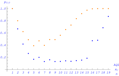
Figure 1: Lot conformance probability $p_{{\cal C}|0}$ for lot conformance limit $x_{\cal C}=\lfloor\mbox{AQL}/100\times N\rfloor$, under $x_{\mbox{\scriptsize ev}}=0$ nonconforming units in sample from lot of size $N=1200$, $a=1.00=b$ (blue), $a=0.57$, $b=37.67$ (orange). Sample sizes from ISO 2859-1, normal inspection, general inspection level II, see table 4.

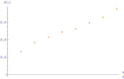
Figure 2: Lot conformance probability $p_{{\cal C}|0}$ for lot conformance limit $x_{\cal C}=\lfloor\mbox{AQL}/100\times N\rfloor$, $\mbox{AQL}=0.04$ in percent, under $x_{\mbox{\scriptsize ev}}=0$ nonconforming units in sample of size $n=315$ from lot of size $N=1200$ for the nine priors $BETA(a,b)$ from table 5. Sample size from ISO 2859-1, normal inspection, general inspection level II, $\mbox{AQL}=0.04$ in percent.

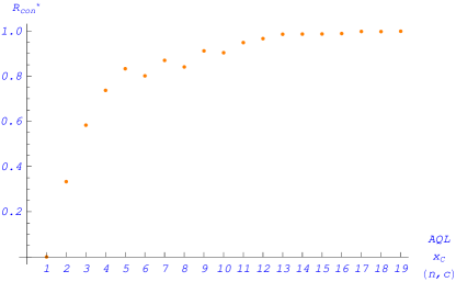
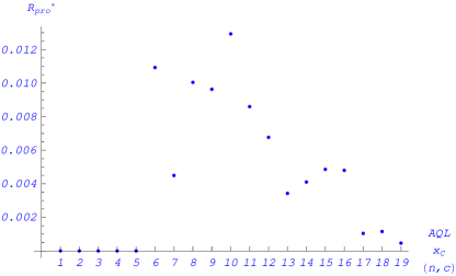
Figure 3: Specific consumer’s risk $R^{\star}_{\mbox{\scriptsize Con}|Y=c}$ and specific producer’s risk $R^{\star}_{\mbox{\scriptsize Pro}|Y=c+1}$, under the lot conformance limit $x_{\cal C}=\lfloor\mbox{AQL}/100\times N\rfloor$, lot size $N=1200$, $a=1.00$, $b=1.00$. AQLs and sampling plans from ISO 2859-1, normal inspection, general inspection level II, see table 4.

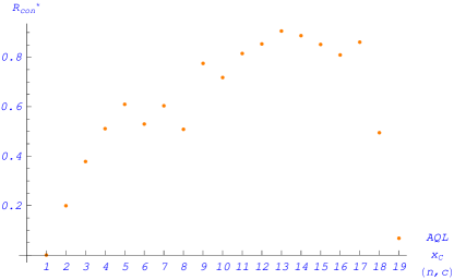
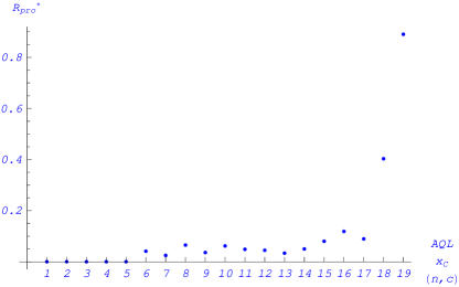
Figure 4: Specific consumer’s risk $R^{\star}_{\mbox{\scriptsize Con}|Y=c}$ and specific producer’s risk $R^{\star}_{\mbox{\scriptsize Pro}|Y=c+1}$, lot conformance limit $x_{\cal C}=\lfloor\mbox{AQL}/100\times N\rfloor$, lot size $N=1200$, $a=0.57$, $b=37.67$. AQLs and sampling plans from ISO 2859-1, normal inspection, general inspection level II, see table 4.

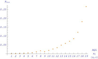
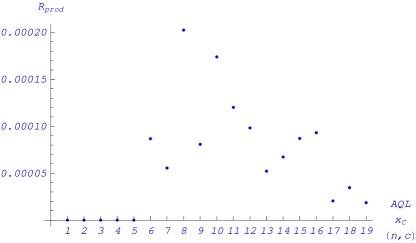
Figure 5: Global consumer’s risk $R_{\mbox{\scriptsize Con}}$ and global producer’s risk $R_{\mbox{\scriptsize Pro}}$, lot conformance limit $x_{\cal C}=\lfloor\mbox{AQL}/100\times N\rfloor$, lot size $N=1200$, $a=1.00$, $b=1.00$. AQLs and sampling plans from ISO 2859-1, normal inspection, general inspection level II, see table 4.

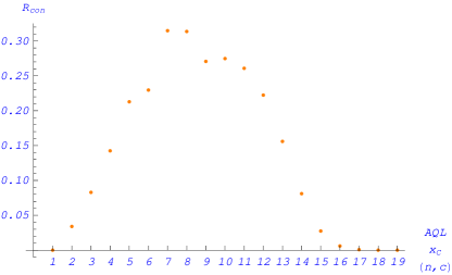
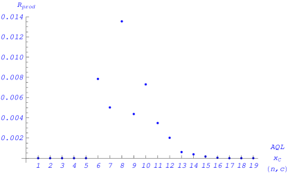
Figure 6: Global consumer’s risk $R_{\mbox{\scriptsize Con}}$ and global producer’s risk $R_{\mbox{\scriptsize Pro}}$, lot conformance limit $x_{\cal C}=\lfloor\mbox{AQL}/100\times N\rfloor$, lot size $N=1200$, $a=0.57$, $b=37.67$. AQLs and sampling plans from ISO 2859-1, normal inspection, general inspection level II, see table 4.

10 Conclusion and outlook

The present paper provides a basic model for the application of the JCGM conformity assessment scheme in acceptance sampling. The mathematical-statistical methodology is developed for attributes sampling. In the next step, the methodology needs to be adapted to variables sampling.

Appendix A The univariate and the bivariate beta-binomial distributions

The univariate discrete distribution defined by the PDF

$$\begin{array}[]{l}\displaystyle f_{n,a,b}(z)\;\;=\;\;{B(z+a,n-z+b)\over B(a,b)}{n\choose z}\quad\mbox{for $z=0,...,n$}\end{array}$$ (19)

is called beta-binomial distribution with parameters $a,b\in(0\mathchar 24635\relax\;+\infty)$ and $n\in\mathbb{N}$, in short beta-binomial distribution $BETA$-$Bi(n,a,b)$. Using the equations (25) and (27) provided by the appendix B, the PDF (19) can be expressed as

$$\begin{array}[]{l}\displaystyle f_{n,a,b}(z)\;\;=\;\;{{a+z-1\choose z}{b+n-z-1\choose n-z}\over{a+b+n-1\choose n}}\;\;=\;\;{{-a\choose z}{-b\choose n-z}\over{-a-b\choose n}}\quad\mbox{for $z=0,...,n$.}\end{array}$$ (20)

The bivariate discrete distribution defined by the PDF

$$\begin{array}[]{l}\displaystyle f_{n_{1},n_{2},a,b}(z_{1},z_{2})\;\;=\;\;{{n_{1}\choose z_{1}}{n_{2}\choose z_{2}}B(a+z_{1}+z_{2},b+n_{1}+n_{2}-(z_{1}+z_{2}))\over B(a,b)}\end{array}$$ (21)

for $z_{i}=0,...,n_{i}$ is called bivariate beta-binomial distribution with parameters $a,b\in(0\mathchar 24635\relax\;+\infty)$ and $n_{1},n_{2}\in\mathbb{N}$, in short addressed as bivariate beta-binomial distribution $BIBETA$-$Bi(n_{1},n_{2},a,b)$. Using the equations (25) and (27) provided by the appendix B, the PDF (21) can be expressed as

$$\begin{array}[]{l}\displaystyle f_{n_{1},n_{2},a,b}(z_{1},z_{2})\;\;=\;\;{{n_{1}\choose z_{1}}{n_{2}\choose z_{2}}\over{n_{1}+n_{2}\choose z_{1}+z_{2}}}{{a+z_{1}+z_{2}-1\choose z_{1}+z_{2}}{b+n_{1}-z_{1}+n_{2}-z_{2}-1\choose n_{1}+n_{2}-z_{1}-z_{2}}\over{a+b+n_{1}+n_{2}-1\choose n_{1}+n_{2}}}\;\;=\\[11.38109pt] \displaystyle{{n_{1}\choose z_{1}}{n_{2}\choose z_{2}}\over{n_{1}+n_{2}\choose z_{1}+z_{2}}}{{-a\choose z_{1}+z_{2}}{-b\choose n_{1}+n_{2}-z_{1}-z_{2}}\over{-a-b\choose n_{1}+n_{2}}}\quad\mbox{for $z_{i}=0,...,n_{i}$.}\end{array}$$ (22)

Proposition 1.

(distributions under beta prior) Let $X$ have the beta distribution $BETA(a,b)$ defined by the PDF (8). Conditional under $X=x$, let $Z_{1}$ and $Z_{2}$ be independent, and let $Z_{i}$ have the binomial distribution $Bi(n_{i},y)$ with $n_{1},n_{2}\in\mathbb{N}$. Then we have:

a)

The unconditional joint distribution of $Z_{1}$ and $Z_{2}$ is the bivariate beta-binomial distribution $BIBETA$-$Bi(n_{1},n_{2},a,b)$ with PDF provided by equations (21) and (22).

b)

For $i=1,2$, the unconditional distribution of $Z_{i}$ is the univariate beta-binomial distribution $BETA$-$Bi(n_{i},a,b)$, and the conditional distribution of $X$ under $Z_{i}=z_{i}$ is the beta distribution $BETA(a+z_{i},b+n_{i}-z_{i})$.

c)

For $z_{1}=0,...,n_{1}$, the conditional distribution of $Z_{2}$ under $Z_{1}=z_{1}$ is the univariate beta-binomial distribution $BETA$-$Bi(n_{2},a+z_{1},b+n_{1}-z_{1})$ with PDF provided by equations (19) and (20).

Proof of of proposition 1.

Consider assertion a). Using the definition (9) of the beta function $B(\cdot,\cdot)$ we obtain

$$f_{Z_{1},Z_{2}}(z_{1},z_{2})\;\;=\;\;\int_{[0\mathchar 24635\relax\;1]}f_{Z_{1},Z_{2}|Y=y}(z_{1},z_{2})f_{Y}(y)\,\mbox{d}y\;\;=\;\;$$

$$\int_{[0\mathchar 24635\relax\;1]}{n_{1}\choose z_{1}}{n_{2}\choose z_{2}}y^{z_{1}+z_{2}}(1-y)^{n_{1}+n_{2}-(z_{1}+z_{2})}{1\over B(a,b)}y^{a-1}(1-y)^{b-1}\,\mbox{d}y\;\;=\;\;$$

$${1\over B(a,b)}\int_{[0\mathchar 24635\relax\;1]}{n_{1}\choose z_{1}}{n_{2}\choose z_{2}}y^{a+z_{1}+z_{2}-1}(1-y)^{b+n_{1}+n_{2}-(z_{1}+z_{2})-1}\,\mbox{d}y\;\;=\;\;$$

$${{n_{1}\choose z_{1}}{n_{2}\choose z_{2}}B(a+z_{1}+z_{2},b+n_{1}+n_{2}-(z_{1}+z_{2}))\over B(a,b)}.$$

Comparing with equation (21) completes the proof of assertion a). Assertion b) is demonstrated analogously. The assertion c) follows from assertions a) and b) with standard formulae of probability calculus.

Appendix B Facts on binomial coefficients and the beta function

For $x\in\mathbb{R}$ and integer $k$ the binomial coeffizient ${x\choose k}$ is defined by

$${x\choose k}\quad:=\quad\left\{\begin{array}[]{ll}0,&\;\mbox{ falls }\;k<0,\\ &\\ 1,&\;\mbox{ falls }\;k=0,\\ &\\ \prod\limits_{i=1}^{k}{x-i+1\over i}\,=\,{\prod_{i=1}^{k}(x-i+1)\over k!},&\;\mbox{ falls }\;k>0.\end{array}\right.$$ (23)

Binomial coefficients $y\choose k$ with $y<0$ are called negative binomial coefficients. We have

$${-x\choose k}\;\;=\;\;(-1)^{k}{x+k-1\choose k}\qquad\mbox{ for }x\in\mathbb{R}\;\mbox{and integer $k$},$$ (24)

and

$${{-x\choose k}{-y\choose n-k}\over{-x-y\choose n}}\;\;=\;\;{{x+k-1\choose k}{y+(n-k)-1\choose n-k}\over{x+y+n-1\choose n}}\quad\mbox{for }x,y\in\mathbb{R},\,n,k\in\mathbb{N}_{0}.$$ (25)

Using the well-known recursion

$$\Gamma(x+1)\;\;=\;\;x\Gamma(x)\quad\mbox{for }x\in(0\mathchar 24635\relax\;+\infty),$$ (26)

for the gamma function we can establish the subsequent relations between the beta function defined by (9) and binomial coefficients:

$$\begin{array}[]{l}\displaystyle B(s+k,t+m)\;\;=\;\;B(s,t){{s+k-1\choose k}{t+m-1\choose m}\over{s+t+k+m-1\choose k+m}}{1\over{m+k\choose m}}\;\;=\\[5.69054pt] \displaystyle B(s,t){{-s\choose k}{-t\choose m}\over{-s-t\choose k+m}}{1\over{m+k\choose m}}\end{array}$$ (27)

for $s,t>0$, $k,m\in\mathbb{N}_{0}$.

References

- (1) Balamurali S, Göb R, Jun CH. Attributes Sampling Schemes in International Standards. In: Ruggeri F, Kenett R, Faltin F (Eds.) Encyclopedia of Statistics in Quality and Reliability, John Wiley & Sons, New York (2008)
- (2) Göb R, Baillie D. Sampling for Nonconformities and Other Issues in the Forthcoming Revision of ISO 2859-2. Quality and Reliability Engineering International, 28 (5): 546-562, 2012.
- (3) Graves SB, Murphy DC, Ringuest JL (2000) Acceptance Sampling and Reliability: the Tradeoff between Component Quality and Redundancy. Computer and Industrial Engineering 38(1): 79-91
- (4) Deros BM, Peng CY, Ab Rahman MN, Sulong AB (2008) Assessing acceptance sampling application in manufacturing electrical and electronic products. Journal of Achievements in Materials and Manufacturing Engineering 31(2): 622-628
- (5) Schilling EG, Neubauer DV (2017) Acceptance Sampling in Quality Control (third edition). Chapman and Hall/CRC, Boca Raton, FL
- (6) United States Department of Defense (1950) Military Standard MIL-STD-105E, Sampling Procedures and Tables for Inspection by Attributes. U.S. Government Printing Office Washington, D. C.
- (7) United States Department of Defense (1958) Military Standard MIL-STD-105E, Sampling Procedures and Tables for Inspection by Attributes. U.S. Government Printing Office Washington, D. C.
- (8) United States Department of Defense (1961) Military Standard MIL-STD-105E, Sampling Procedures and Tables for Inspection by Attributes. U.S. Government Printing Office Washington, D. C.
- (9) United States Department of Defense (1963) Military Standard MIL-STD-105E, Sampling Procedures and Tables for Inspection by Attributes. U.S. Government Printing Office Washington, D. C.
- (10) United States Department of Defense (1989) Military Standard MIL-STD-105E, Sampling Procedures and Tables for Inspection by Attributes. U.S. Government Printing Office Washington, D. C.
- (11) International Organization for Standardization ISO 2859-1:1999 Sampling procedures for inspection by attributes – Part 1: Sampling schemes indexed by acceptance quality limit (AQL) for lot-by-lot inspection. International Organization for Standardization, Geneva, 1999.
- (12) International Organization for Standardization. ISO 2859-2:2020 Sampling procedures for inspection by attributes – Part 2: Sampling plans indexed by limiting quality (LQ) for isolated lot inspection. International Organization for Standardization, Geneva, 2020.
- (13) Dodge HF (1969a) Notes on the Evolution of Acceptance Sampling Plans, Part I. Journal of Quality Technology 1(2): 77-88
- (14) Dodge HF (1969b) Notes on the Evolution of Acceptance Sampling Plans, Part II. Journal of Quality Technology 1(3): 155-162
- (15) Dodge HF Notes on the Evolution of Acceptance Sampling Plans, Part III. Journal of Quality Technology 1(4): 225-232
- (16) Dodge HF. Notes on the Evolution of Acceptance Sampling Plans, Part IV. Journal of Quality Technology 2(sup1): 1-8, 1969
- (17) Dodge HF, Romig HG. Sampling Inspection Tables(second edition). John Wiley & Sons, New York, 1959.
- (18) Duncan AJ. Quality Control and Industrial Statistics (fourth edition). Richard D. Irwin, Homewood Ill, 1974
- (19) Feigenbaum AV. Total Quality Control. McGraw-Hill, New York, 1961.
- (20) Godfrey AB, Mundel AB Guide for Selection of an Acceptance Sampling Plan. Journal of Quality Technology, 16(1): 50-55, 1984.
- (21) Liepiņa R, Lapiņa I, Mazais J. Contemporary issues of quality management: relationship between conformity assessment and quality management. Procedia – Social and Behavioral Sciences, 110: 627-637, 2014.
- (22) Pendrill LR. Using measurement uncertainty in decision-making and conformity assessment. Metrologia 51(4): 206-218, 2014.
- (23) Joint Committee on Guides in Metrology (JCGM). JCGM 106:2012 Evaluation of Measurement Data – The role of measurement uncertainty in Conformity Assessment. Joint Committee on Guides in Metrology (JCGM), 2012.
- (24) International Organization for Standardization ISO 3534-1:2006 Statistics – Vocabulary and symbols – Part 1: General statistical terms and terms used in probability. International Organization for Standardization, Geneva, 2006.
- (25) International Organization for Standardization ISO 3534-2:2006 Statistics – Vocabulary and symbols – Part 2: Applied statistics. International Organization for Standardization, Geneva, 2006.
- (26) Peach P, Littauer SB. A Note on Sampling Inspection. The Annals of Mathematical Statistics, 17: 81-84, 1946.
- (27) Göb R, Lurz K. Design and analysis of shortest two-sided confidence intervals for a probability under prior information. Metrika 77: 389-413, 2014.
- (28) Hald A. Statistical theory of sampling inspection by attributes. Academic Press, London, New York (1981)
- (29) Godfrey J, Andrews R A Finite Population Bayesian Model for Compliance Testing. Journal of Accounting Research 20(2): 304–315, 1982.
- (30) Berg N. A Simple Bayesian Procedure for Sample Size Determination in an Audit of Property Value Appraisals. Real Estate Economics 34(1): 133–155, 2006.
- (31) Kendrick T Identifying and Managing Project Risk: Essential Tools for Failure-Proofing Your Project. 2nd ed. AMACOM, New York (2009)
- (32) Kim B, Reinschmid KF. Probabilistic Forecasting of Project Duration Using Bayesian Inference and the Beta Distribution. Journal of Construction Engineering and Management, 135(3): 178-186, 2009.
- (33) Eschmann M, Stamey J, Young P, Young, D. (2019) Bayesian Approach to Ranking and Selection for a Binary Measurement System. Open Journal of Statistics, 9: 436-444, 2019.
- (34) Corless JC Assessing Prior Distributions for Applying Baysian Statistics in Auditing. The Accounting Review 47 (3): 556–566, 1972.
- (35) Hogarth RM Cognitive Processes and the Assessment of Subjective Probability Distributions. Journal of the American Statistical Association 70: 271–289, 1975.
- (36) Kadane JB, Dickey JM, Winkler RL, Smith WS, Peters SC Interactive Elicitation of Opinion for a Normal Linear Model. Journal of the American Statistical Association 75: 845–854, 1980.
- (37) Chaloner KM, Duncan GT Assessment of a Beta Prior Distribution: PM Elicitation. The Statistician 32: 174–180, 1983.
- (38) O’Hagan A Eliciting Expert Beliefs in Substantial Practical Applications. The Statistician 47(1): 21–35 (1998)
- (39) Walls L, Quigley J Building Prior Distributions to Support Bayesian Reliability Growth Modeling Using Expert Judgment. Reliability Engineering and System Safety 74(2): 117–128 (2001)
- (40) Blocher E, Robertson JC Bayesian Sampling Procedures for Auditors: Computer-Assisted Instruction. The Accounting Review 51(2): 359–363 (1976)
- (41) Garthwaite PH, O’Hagan A Quantifying Expert Opinion in the UK Water Industry: An Experimental Study. The Statistician, 49: 455–477 (2000)