P² Explore: Efficient Exploration in Unknown Clustered Environment with Floor Plan Prediction

Abstract

Robot exploration aims at constructing unknown environments and it is important to achieve it with shorter paths. Traditional methods focus on optimizing the visiting order based on current observations, which may lead to local-minimal results. Recently, by predicting the structure of the unseen environment, the exploration efficiency can be further improved. However, in a cluttered environment, due to the randomness of obstacles, the ability for prediction is limited. Therefore, to solve this problem, we propose a map prediction algorithm that can be efficient in predicting the layout of noisy indoor environments. We focus on the scenario of 2D exploration. First, we perform floor plan extraction by denoising the cluttered map using deep learning. Then, we use a floor plan-based algorithm to improve the prediction accuracy. Additionally, we extract the segmentation of rooms and construct their connectivity based on the predicted map, which can be used for downstream tasks. To validate the effectiveness of the proposed method, it is applied to exploration tasks. Extensive experiments show that even in cluttered scenes, our proposed method can benefit efficiency.

I Introduction

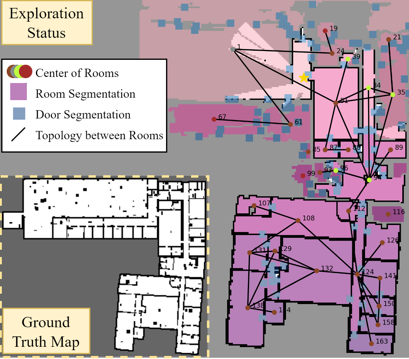
Figure 1: Illustration of the proposed method. The bottom left shows the ground truth of the 2D grid map of the environment, while the right side displays the exploration status at a specific moment. During exploration, we first obtain the floor plan by denoising and then we predict the floor plan. Besides, the segmentation of rooms (purple area) and their topological connectivity (black line) is extracted, which can be used to accelerate the exploration.

The primary goal of robotic systems is to interact with the physical world based on observational information, such as tasks like manipulation [1], navigation [2, 3] and exploration [4, 5]. This physical environment can be classified into two categories based on its initial status: known and unknown. In fully known environments, it is possible to design algorithms to achieve optimal strategies. For example, using a fully observed map, a near-optimal path can be found from the start point to the destination using various path planning algorithms [6]. However, in partially observed environments, these algorithms are limited to current observations, which can lead to locally optimal solutions.

Robot exploration, also called active Simultaneous Localization and Mapping (SLAM), aims at reconstructing the environment, which is widely studied these days [4, 5, 7, 8, 9, 10, 11, 12, 3]. One form of exploration involves the complete reconstruction of the environment [4, 5, 7, 8, 9]. In this case, the robot uses 2D or 3D sensors to plan its motion trajectory in order to build a map of the environment. Another form focuses on conducting minimal exploration until the pre-defined goal can be achieved. For example, to perform point-to-point navigation in unknown environments [3, 11, 12, 10], exploration is utilized to find a traversable path from the starting point to the destination. For both forms, a common evaluation metric is to minimize the length of the robot’s trajectory.

To achieve exploration, most of the methods focus on using the current observed environment to determine the next goal[5, 13, 14]. In [14], a greedy algorithm is employed. To achieve exploration, the next best view (NBV) is selected by calculating the information gain and navigation cost for frontiers in the current map. In [5, 13], the author considers constructing a visiting sequence of all frontiers as a Traveling Salesman Problem (TSP). By optimizing the visiting order of the current observations, the exploration can be accelerated. The distributed form of this problem is studied in [15, 16]. However, these methods focus on the current observed environment and it is hard to obtain an optimal trajectory.

Therefore, a question arises: In the exploration task, is it possible to find the global shortest trajectory? Inspired by the map coverage problem [17], for a fully known environment, we can find an optimal trajectory to achieve coverage of the environment. The primary difference between exploration and map coverage lies in whether prior information about the environment is available. Therefore, if we can predict the occupancy of the unobserved parts based on a partially observed environment, it would be possible to generate an optimal trajectory for exploration. However, a perfect map predictor does not exist. The farther a location is from the observed area, the higher the probability of making an error in predicting its occupancy status. Therefore, a key research question is how to utilize an imperfect map predictor to accelerate exploration.

Previous works have explored how to use map predictors to enable exploration or navigation in unknown environments [18, 9]. Indoor environments can be categorized into two types: floor plans and clustered environments. Floor plans are the structure of walls in indoor scenes. In [19, 20], geometry-based methods are used to achieve floor plan prediction. However, traditional methods face challenges in generalization, leading to a greater focus on using deep learning techniques. In [21, 22], floor plans are predicted using an auto-regressive sequence prediction method. In [9], a lightweight neural network is used as a map predictor, and a deep reinforcement learning-based method is proposed for efficient exploration. However, current methods mainly focus on map prediction in size-limited and noise-free scenes, which rarely appear in the real world, leading to a constrained application.

Some other researchers focus on predicting the clustered scenes, where the presence of furniture and other objects results in irregular structures in the constructed map. However, due to this irregularity, the effectiveness of map prediction is often poor. In [10, 11, 23], the robot is equipped with a 2D LiDAR to perform point-to-point navigation in an unknown environment. Map predictors are used to forecast potential navigable paths. However, the range of prediction is limited to areas very close to the current map. As a result, the effectiveness of map prediction is poor, offering only a modest acceleration for the downstream task. Even when equipped with advanced sensors, such as RGB-D cameras, only the nearby portions of the map can be predicted [24, 25, 26, 27, 28].

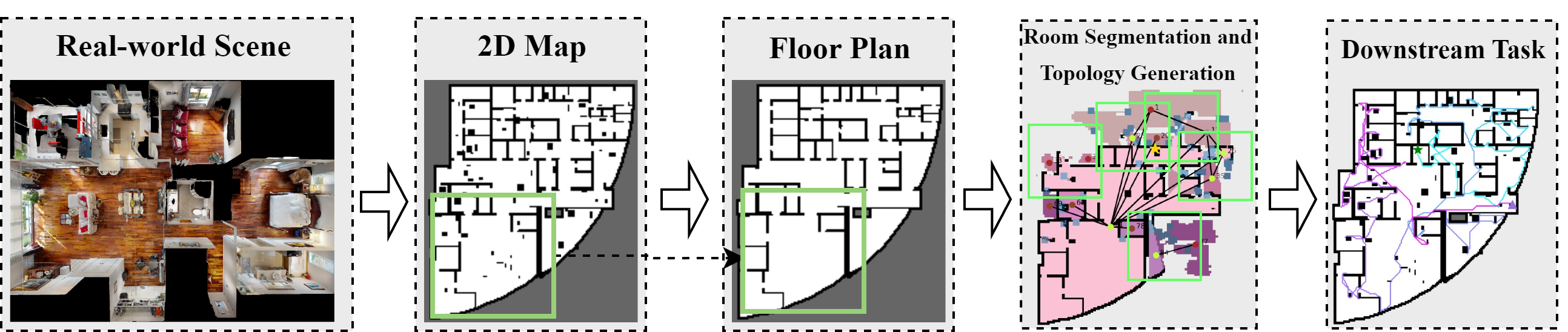
Figure 2: Illustration of the framework of the proposed method. For real-world scenes, there will be various obstacles in the 2D grid map. To achieve efficient map prediction, we denoise the 2D map first and then perform prediction based on floor plan. Finally, the predicted map can be used to extract room segmentation and their topology, which provides guidance for the downstream tasks.

In our work, we minimize the gap between predicting maps for clustered scenarios of any size and current research. We propose a framework called P² Explore. Firstly, we train a neural network to perform floor plan extraction in a clustered map. Then, real-world floor plan datasets are used to train another network for predicting local maps. Additionally, we design an algorithm to combine predictions from different positions, enabling the generation of a global predicted map. As a result, our algorithm can be extended to maps of any scale. Furthermore, we perform region segmentation based on the predicted map, extracting the specific locations of individual rooms and automatically generating the topological connectivity between them, which can be used for downstream tasks. Leveraging the predicted rooms and connectivity, we apply our approach to exploration and navigation tasks in unknown environments. The illustration for the proposed method can be found in Fig. 2. Our main contributions are

• A map prediction algorithm for clustered environment with unlimited size is proposed, enabling both room segmentation and connectivity prediction.

• Algorithms are designed to integrate map prediction with exploration and navigation tasks in unknown environments.

• The effectiveness of the algorithm is validated in both simulations and real-world environment with noise.

II Methodology

II-A Map predictor

In this work, we focus on the task of map prediction in 2D environment. We define the observed map as $X\in\mathcal{C}^{H\times W}$, where $\mathcal{C}=\{0,100,255\}$, and $H/W$ is the height/width of the map. For each cell in $X$, different numbers are used to represent its state, where 0 is occupied, 100 is unknown, and 255 is free. A frontier $f_{i}$ is defined as the boundary between free and unknown spaces. Local map around $f_{i}$ is defined as

$$X(f_{i})=\{x\ \big{|}\ ||x-f_{i}||_{1}\leq R,x\in X\},$$ (1)

where $R$ is the range of local map. In this work, $R$ is set to 12 m, which is the same as the range of 2D LiDAR used in the real world experiments.

For indoor environments, furniture such as sofas, chairs, and various objects of different shapes located in arbitrary positions create irregular obstacle areas on $X$. As a result, it is difficult to perform map prediction directly on it. Therefore, we first consider denoising $X$ into a floor plan $\tilde{X}$. A light-weight neural network is used to perform denoising and the detailed information will be presented in Section II-A2.

Then, we propose our map predictor based on this denoised map $\tilde{X}$. Assuming that the fully observed floor plan around $f_{i}$ can be denoted as $\hat{X}_{gt}(f_{i})$. For the map predictor, our goal is to find parameters $\theta$ of a neural network that can minimize the error between predicted floor plan $\hat{X}(f_{i})=\psi_{\theta}(\tilde{X}(f_{i}))$ and $\hat{X}_{gt}(f_{i})$

$$\arg\min_{\theta}\sum_{i}|\hat{X}(f_{i})-\hat{X}_{gt}(f_{i})|_{p},$$ (2)

where in this work, we use $p=1$.

II-A1 Dataset Generation

Similarly with [22], we can obtain different scenes from KTH floor plan dataset[29]. This dataset describes the floor plan in the form of line segments, specifying the start and end points. Each line segment can be categorized into three types: wall, window, and door. The locations of walls within the environment indicate the traversability of the scene. Then, we map the positions of walls in each floor plan to a grid map, where each grid cell represents 0.2 m in the real world.

In this dataset, walls may not be connected, making it difficult to accurately identify the interior of walls. To address this, we first connect endpoints of different line segments that are less than 0.4 m apart. Next, by combining the flood-fill algorithm with manual corrections, we can identify the interior of each scene. Each grid cell is then assigned a label as either occupied, free, or unknown.

Due to that in the KTH floor plan dataset, similar floor plans will appear in two different maps. For example, they could be different floors in the same building. Therefore, if we shuffle the entire dataset, training data and testing data will share some similar floor plans. To avoid this, we remove those similar plans and obtain 140 different floor plans. The average and maximum size of the scene are 745.59 m² and 4548.48 m². To simulate irregular obstacles in the real world, we add random obstacles of varying sizes and quantities to each map to represent real-world environments.

Then, a robot equipped with a LiDAR with a range of 12 m is randomly placed at a point in the map. Initially, the robot can only observe the nearby information. We assume the robot performs a virtual exploration based on the Next Best View (NBV) strategy [14]. Each time, the robot selects a frontier $f_{i}$ as the goal for exploration. At this point, the local map $X(f_{i})$ around $f_{i}$ can be obtained. It is possible to obtain the ground truth floor plan $\tilde{X}_{gt}(f_{i})$ using $X(f_{i})$. Additionally, we can also acquire the ground truth fully observed floor plan $\hat{X}_{gt}(f_{i})$. Thus, we can obtain triplets like $(X(f_{i}),\tilde{X}_{gt}(f_{i}),\hat{X}_{gt}(f_{i}))$. In different scenes and different steps of exploration, we can obtain similar data, which is our training dataset.

II-A2 Training Details

For the original dataset, we divide it into training, testing, and validation sets according to different scenes, with proportions of 70%, 15%, and 15%, respectively. Since we predict maps with a size of 12 m around the robot, the original image input size is 120$\times$120.

Firstly, we train a map denoising module. Since the denoising process needs to consider both low-frequency floor plan information and high-frequency noise, we choose UNet++ [30] as the backbone, which captures features at different levels. The number of convolutional kernels in each part is set to 16, 32, 64, 128, and 256. The original map $X(f_{i})$ is taken as the input, and the network outputs the denoised floor plan $\tilde{X}(f_{i})$. The label is set as $\tilde{X}_{gt}(f_{i})$ and the loss is L1-norm between these two pictures.

Secondly, the floor plan prediction module $\psi_{\theta}$ is trained. Due to the floor plan containing low-frequency information only, our network architecture is UNet [31] which is more efficient than UNet++. $\psi_{\theta}$ takes the input as $\tilde{X}_{gt}(f_{i})$ and predicts $\hat{X}_{gt}(f_{i})$. In the inference procedure, we use $\tilde{X}(f_{i})$ as the input of $\psi_{\theta}$.

For the two networks, before inputting the images into the network, they are normalized into a range of -1 to 1. We set the optimizer to Adam with a learning rate of 0.0005, train for 300 epochs, and save the network that performs best on the validation set as the final result.

II-A3 Obtain the Global Predicted Map

The predicted local floor plan $\hat{X}(f_{i})$ is convert to a range of 0 to 255 firstly, and we classify values less than 80 as occupied, greater than 120 as traversable, and the remaining values as unknown. To enable map prediction for environments of any size, we use the local map around each frontier as input to obtain the local predicted map. Assuming that in the current partially observed map, we can obtain some clustered frontiers $f_{i},i=1\cdots n$. The local maps around $f_{i}$ is $X(f_{i})$. Based on the trained denoising module and map predictor $\psi_{\theta}$, we can obtain the predicted map $\hat{X}(f_{i})$. The detail algorithm for merging the local predicted maps can be found in Algorithm 1.

Input: original map $X$, frontiers $\{f_{i}\}$, predicted local maps $\{\hat{X}(f_{i})\}$

Output: predicted global map $\hat{X}$

1 $\hat{X}$ $\leftarrow$ $X$

2 Unknown_Index $\leftarrow$ $\texttt{where}(X=100)$

3 for $\hat{X}(f_{i})\in\{\hat{X}(f_{i})\}$ do

4       Predicted_Index $\leftarrow$ $\texttt{where}(\hat{X}(f_{i})\neq 100)$

5       Index $\leftarrow$ $\text{Unknown\_Index}\cap\text{Predicted\_Index}$

6       $\hat{X}[\text{Index}]$ $\leftarrow$ $\hat{X}(f_{i})[\text{Index}]$

Algorithm 1 Merge Local Prediction

For each local predicted map $\hat{X}(f_{i})$, the valid prediction information (occupied or traversable) is added to the corresponding location in the global predicted map $\hat{X}$. Additionally, we retain the already observed information in the original map.

II-A4 Room Segmentation and Topology Generation

Although using the predicted map directly can accelerate tasks like exploration to some extent, the noise present in the predictions makes it difficult to develop effective algorithms for more advanced tasks. In this work, we further abstract the predicted information by extracting rooms and the topological connectivity between them from the predicted map $\hat{X}$. This will provide more accessible and practical guidance for tasks compared with the rough predicted information.

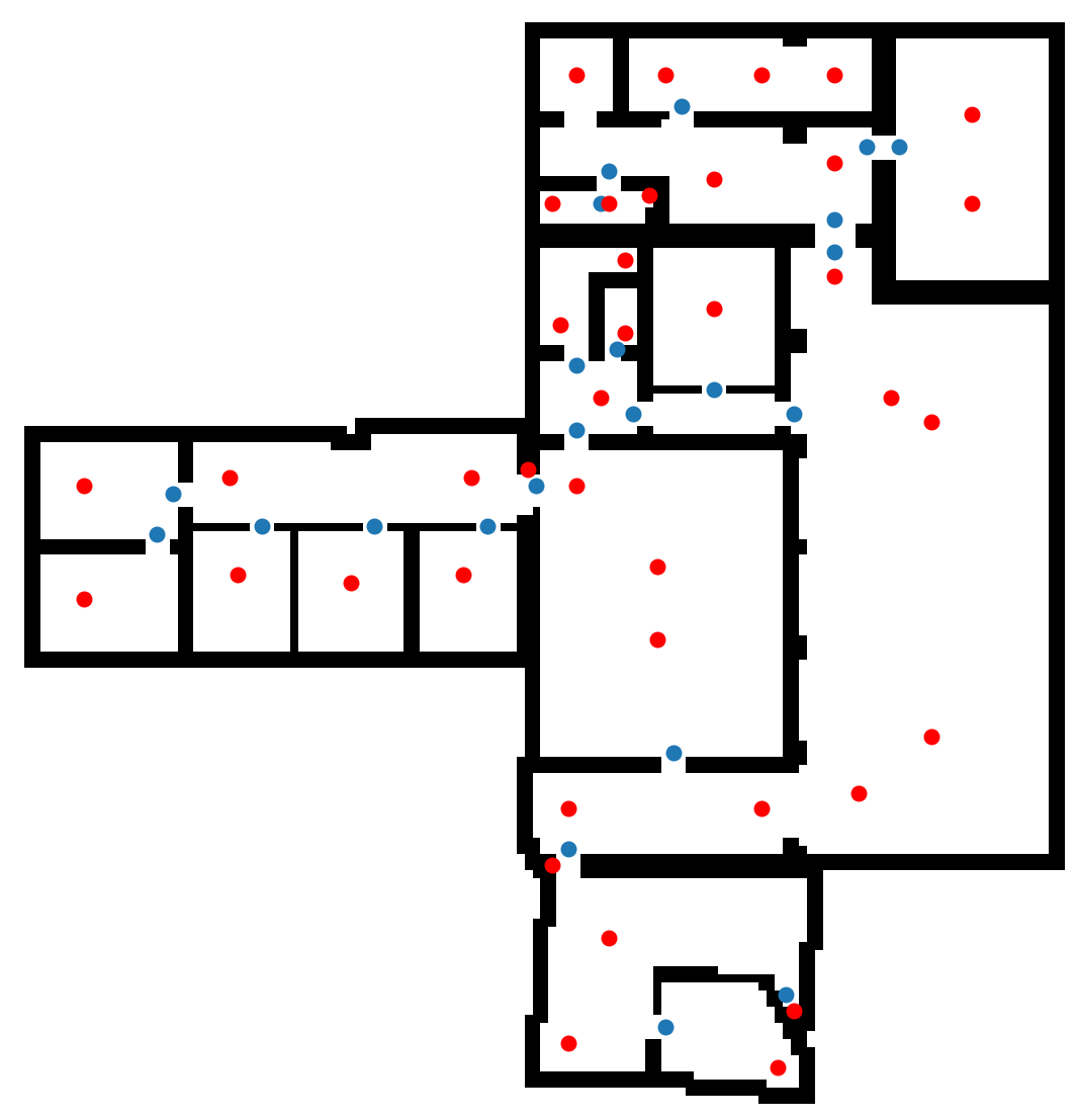
(a)

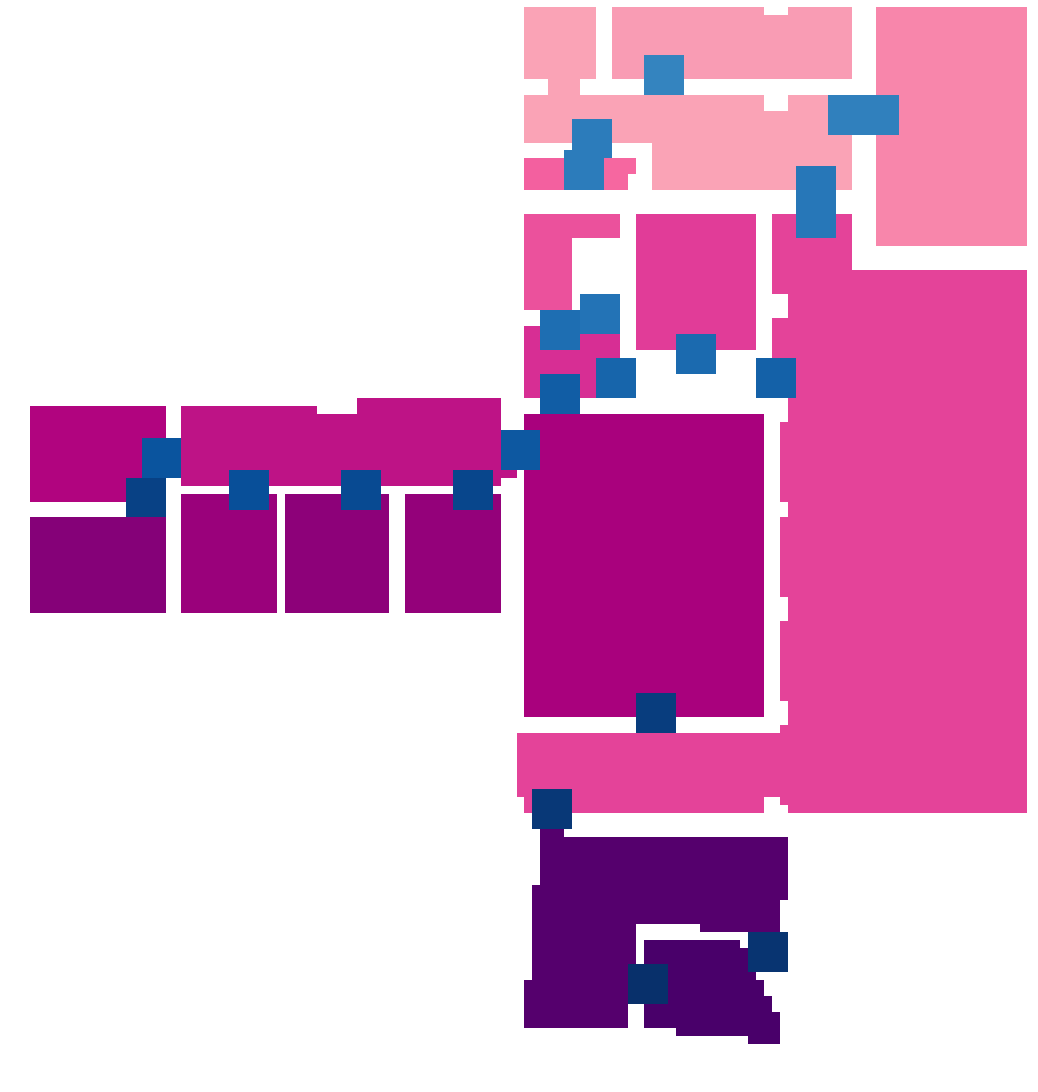
(b)

Figure 3: (a) Obtained poses of rooms and doors. The red point represent the poses of rooms. The blue points represent the poses of doors. (b) Created segmentation of the scene. The red and blue areas represent different rooms and doors respectively.

For map $\hat{X}$, it can be converted into a 2D distance transform map $D$ by considering the distance from each point to the nearest obstacle. Assuming that the value of grid cell $(u,v)$ in $D$ can be denoted by $D(u,v)$, saddle points $P^{sadd}$ and local maxima points $P^{max}$ in $D$ can be useful in finding the position of doors and rooms [7]. $P^{sadd}$ and $P^{max}$ can be obtained by considering the determinant of hessian matrix $H$ of $D(u,v)$

$$|H|=D_{uu}(u,v)D_{vv}(u,v)-D^{2}_{uv}(u,v).$$ (3)

$P^{sadd}$ and $P^{max}$ are defined as

$$\left\{\begin{array}[]{l}(u,v)\in P^{sadd},\text{if}\ |H|<-0.4\\ (u,v)\in P^{max},\text{if}\ |H|>0\ \text{and}\ D_{uu}<-0.4,\end{array}\right.$$ (4)

where $|H|$ is the determinant of $H$. Theoretically, setting $|H|<0$ should yield a saddle point. However, in practical experiments, we find that setting $|H|$ to a value slightly less than zero can help eliminate saddle points caused by noise in the maps. The same approach applies to finding local extremum. The detected $P^{sadd}$ and $P^{max}$ of a fully observed map are illustrated in Fig. 3a.

The calculation of room segmentation and topological connectivity based on the $\hat{X}$ is shown in Algorithm 2. Based on the $P^{sadd}$, $P^{max}$, and $\hat{X}$, we first initialize a segmentation map $S$ with all zeros. Then, the positions of predicted doors are labeled with -1. Due to errors in the saddle points extraction, there may be multiple predicted saddle points corresponding to a single door in the actual environment. Therefore, we map overlapping doors to a single one in the final map and assign each door with a unique negative value. By adding doors to $\hat{X}$, we can segment the predicted map into different rooms. Each room contains connected traversable areas with a value of 255. Next, starting from points $P^{max}$, we use the flood-fill algorithm to obtain the grid cell indices of the current room and add the corresponding indices to $S$. Finally, we construct an adjacent matrix $\mathcal{A}$. For rooms connected by a door, we mark them as connected in $\mathcal{A}$. The illustration of segmentation can be found in Fig. 3b The created topology connectivity of a partially observed map can be found in Fig. 1.

Input: $P^{sadd}$, $P^{max}$, predicted map $\hat{X}$, size of doors $r$

Output: adjacent matrix of rooms $\mathcal{A}$, segmentation map $S$

1 $S$ $\leftarrow$ $\texttt{ZEROS}(\hat{X}.\text{shape})$, RLabel $\leftarrow$ $1$

2 for $p\in P^{sadd}$ do

3       $S(i)=-1,\hat{X}(i)=-1,\forall||i-p||_{1}<r$

4      

5$S,N_{door}$ $\leftarrow$ $\texttt{AssignUniqueLabel}(S)$

6 for $p\in P^{max}$ do

7       if $S[p]=0$ then

8             $S$ $\leftarrow$ $\texttt{FILL}(S,\hat{X},p,\text{RLabel})$, $\text{RLabel+=}1$

9            

10      

11$\mathcal{A}$ $\leftarrow$ $\texttt{ZEROS}(\text{RLabel}-1,\text{RLabel}-1)$

12 for $i\in\texttt{Range}(1,N_{door})$ do

13       $\mathcal{A}$ $\leftarrow$ $\texttt{FindAdjacentRoom}(S,-i,\mathcal{A})$

return $\mathcal{A}$,$S$

Algorithm 2 Create Segmentation and Topology

In the following sections, we will demonstrate how to utilize the predicted segmentation and topological connectivity to accelerate exploration and navigation tasks.

II-B Application of Map Predictor in Exploration

Based on the method of predicting the floor plan from a noisy 2D grid map, we apply it to exploration and navigation tasks in unknown environments.

In the exploration task, we consider a simple strategy. Specifically, in indoor environments, the robot often needs to fully explore one room before moving to another [32]. Therefore, we focus on assigning the next goal of the robot within the same room. Assuming that during exploration, the pose of the robot is $p(t)$, our method is similar to NBV-based strategy, which can be denoted as

$$U(f_{i})=kI(f_{i})\exp^{-\lambda d(f_{i},p(t))}-C(f_{i},p(t)),$$ (5)

where $k$ and $\lambda$ are two hyper-parameters. $I(f_{i})$ is the predicted information gain, which can be defined as the predicted free space area near $f_{i}$ and the range is defined as 1 m. $d(f_{i},p(t))$ refers to the distance between the room containing $f_{i}$ and the room containing $p(t)$ on the predicted topology $\mathcal{A}$. The distances between each node in $\mathcal{A}$ is defined as 1. $C(f_{i},p(t))$ is the navigation cost between $f_{i}$ and $p(t)$. The robot will choose frontier with maximum utility as its next goal.

Equ. 5 is closely related to the traditional NBV-based exploration [14]. In this work, we assign different weights to the frontiers of each room based on their distance from the current room in the room topology, and the information gain is calculated based on the predicted map. In section III-B, we will discuss the effectiveness of the proposed method.

II-C Application of Map Predictor in Navigation

When performing navigation tasks in unknown environments, the predicted floor plan can also be effective. We assume that the robot is currently at point $p(t)$ and the pose of target $p_{\text{targ}}$ in the robot’s coordinate is already known. The goal of the robot is to find the shortest path to reach the target point. Since the environment is unknown, the robot must perform minimal exploration of the environment first.

Based on the predicted floor plan, we propose a strategy considering frontiers. Inspired by the A* path planning algorithm, for any point $p$, the path length from $p(t)$ to $p_{\text{targ}}$ through $p$ can be denoted as

$$C(p(t),p,p_{\text{targ}})=C(p(t),p)+\hat{C}(p,p_{\text{targ}}),$$ (6)

where $\hat{C}(p,p_{\text{targ}})$ is the estimated navigation cost from $p$ and $p_{\text{targ}}$. If we could accurately predict the value of $\hat{C}(p,p_{\text{targ}})$ and select the next goal among all action spaces each time, we would be able to find the shortest path. However, since the environment is unknown, we can only obtain an estimated value of it. We use the predicted floor plan to obtain $\hat{C}(p,p_{\text{targ}})$. The traversable and obstacle areas in $\hat{X}$ are retained and all unknown areas are set as traversable. Then, the distance $\hat{C}$ can be obtained based on the modified floor plan. In section III-C, we will discuss the effectiveness of implementing floor plan prediction into navigation.

III Experiments

We study the application of floor plan prediction in exploration and navigation tasks. In simulations, a robot is equipped with a 12 m range LiDAR. Besides, the localization system is assumed to be perfect, which is similar to [5]. Training of two neural networks and simulations are conducted using AMD Ryzen 3900X CPU, 64 GB RAM, and NVIDIA RTX 3090 GPU. In Equ. 5, $k$ is set to 0.05 and $\lambda$ is set to 1.

III-A Case Study of The Map Prediction Results

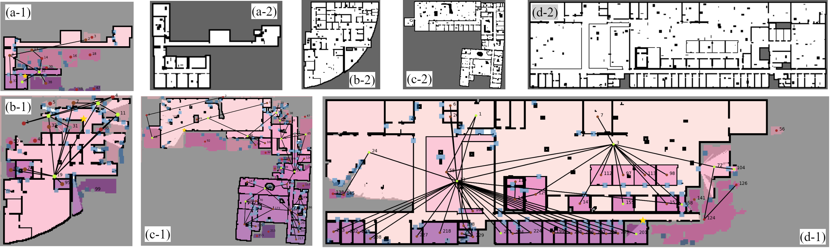
Figure 4: Illustration for map prediction in different scenes. The first picture in each group is the denoised floor plan and predicted map. The second picture is the ground truth scenes. The scene is getting larger from (a) to (d). Besides, in (c), compared with the result illustrated in Fig. 1, we add more noise with various sizes in the scene and we can find that our method fails in removing all the noise.

The results of the proposed method in different scenes can be found in Fig. 4. We choose four typical scenes in the test set for evaluation. The areas of four scenes are 228.52, 604.84, 1126.44, and 2577.4 m². In (a), the scene is relatively small in size, and only a few rooms are in the scene. Our methods can predict the existence of unseen rooms, while the detailed shapes are inaccurate. For (b), there are multiple small rooms in the scene, and our method can perform the prediction task successfully. In (c), we add various obstacles in the scene, and the denoising module starts to fail in predicting some of the floor plan. (d) has a complex structure, and room segmentation module begins to fail in some large rooms. Overall, our method can make reasonable predictions in various scenes and provide guidance for the downstream task.

III-B Exploration Results

Out of all 140 scenes, 21 scenes are selected as the test set. For smaller maps (less than 200  m²), exploration can be completed quickly even without prediction, making comparisons less meaningful. Therefore, we focus on studying exploration efficiency in medium-sized (200–600 m²) and large-sized scenes (greater than 600 m²). In the test set, there are 7 scenes for each of the two categories. Exploration efficiency is evaluated under two different conditions. The first condition is exploration in pure floor plans, where the map predictor has a perfect and noise-free partially observed map as input. The second condition involves exploration with random noise in the map, where we first remove the noise from the observed map and then predict the floor plan based on the extracted data. Comparison and ablation studies are conducted to validate the proposed method. Two methods are selected for comparison. The first one is NBV [14], where the next goal for the robot is selected as the frontier with maximum utility. The second one is TSP[5, 13], which can be seen as the state-of-the-art (SOTA) method. In TSP, the robot considers the distribution of all frontiers during each step and formulates a Traveling Salesman Problem (TSP) to traverse all the frontiers.

TABLE I: Comparison and ablation studies of exploration efficiency. Methods with “*” and “#” are comparison and ablation experiments respectively. Evaluation metric: path length (m).

	Pure Floor Plan		Noised Map
Method	Middle (200-600 m2)	Large ($>$600 m2)	Middle (200-600 m2)	Large ($>$600 m2)
NBV*	200.19 (69.87)	442.73 (192.70)	254.09 (66.14)	595.54 (284.94)
TSP*	195.63 (44.67)	436.89 (208.50)	247.99 (77.62)	589.67 (268.12)
NoPre#	190.44 (56.93)	430.94 (184.94)	244.70 (76.29)	578.21 (250.86)
TD#	/	/	251.29 (83.48)	576.37 (250.10)
Ours	180.11 (59.87)	421.96 (195.22)	240.83 (78.38)	573.63 (253.09)

The detailed results can be found in Table I. In all four different types of scenarios, TSP shows better exploration efficiency than NBV. However, compared to the current SOTA methods TSP, the prediction-based approach still offers some improvement. In floor plan exploration, for middle scenes, our method reduces the distance by 15.52 m compared to TSP, resulting in a 7.93% improvement. For large scenes, our method also reduces the distance by 14.93 m. For noised maps, our method shortens the distance by 7.16 m and 16.04 m compared to TSP. It can be seen that our method achieves greater improvements in floor plan-based exploration than in the noised map. This is because the map contains some noise, which first affects the accuracy of the floor plan prediction. Additionally, the designed exploration strategy is not perfect, so even if the floor plan is predicted accurately, the exploration strategy does not make full use of it.

We conduct ablation experiments to validate the effectiveness of the prediction. The result can be found in Table I. In TD, a traditional denoising method based on RANSAC is used. In NoPre, the predicted information in Equ. 5 is replaced with current observed maps $X$. Compared with NoPre, we can find that the predicted information can accelerate exploration, especially in pure floor plan scenes. This can be attributed to the superiority in map prediction ability in noise-free scenes. Compared with TD, our denoising module is better than traditional methods, leading to an increase in exploration efficiency.

III-C Navigation Results

The ability to use predicted information for navigation is validated in a large scene. In smaller and simpler scenarios, greedily selecting the next goal as the point closest to the target can be efficient. To demonstrate the effectiveness of map prediction, we choose a more complex scene and set the start point $p(t)$ and target $p_{\text{targ}}$ far apart.

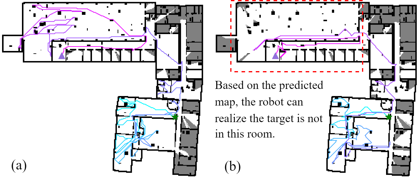
Figure 5: Illustration for navigation results. The green star is the start point for navigation and the purple triangle is the target. (a) Navigation based on greedy frontier-based method. (b) Navigation based on floor plan prediction.

We compare the map prediction-based method with traditional navigation methods in unknown environments, where the distance from point $p$ to $p_{\text{targ}}$ in Equ. 6 is determined based on the currently observed map. The results can be found in Fig. 5. The traveling distance of our method is 376.32 m, while the distance of the traditional method is 500.78 m. Our method shortened the distance by 24.85%. The reason why our method achieves significant improvement is that it can predict a complete room structure after exploring just a portion of the room. This allows us to determine whether the target is inside the current room, thereby providing guidance for the direction of exploration. However, it is important to note that since predictions may sometimes be inaccurate, in some simpler scenarios, incorrect predictions can result in a longer path to the target compared to a greedy algorithm.

III-D Real-world Experiments

Since the training set is based on the KTH floor plan dataset, the effectiveness and generalization performance remains in doubt in real-world scenes. Therefore, we validate our proposed method in a real-world laboratory scene. We first use a Turtlebot equipped with an RPLIDAR A2 LIDAR (range 12 m) to reconstruct the environment. Cartographer is used to obtain a cluttered 2D grid map of the area. Due to odometry errors and the limitations of the mapping algorithm, the resulting 2D map is imperfect. Therefore, we remove the noise caused by the drift of the robot from the map, retaining information about obstacles and other features. Then, we perform simulated exploration in the map.

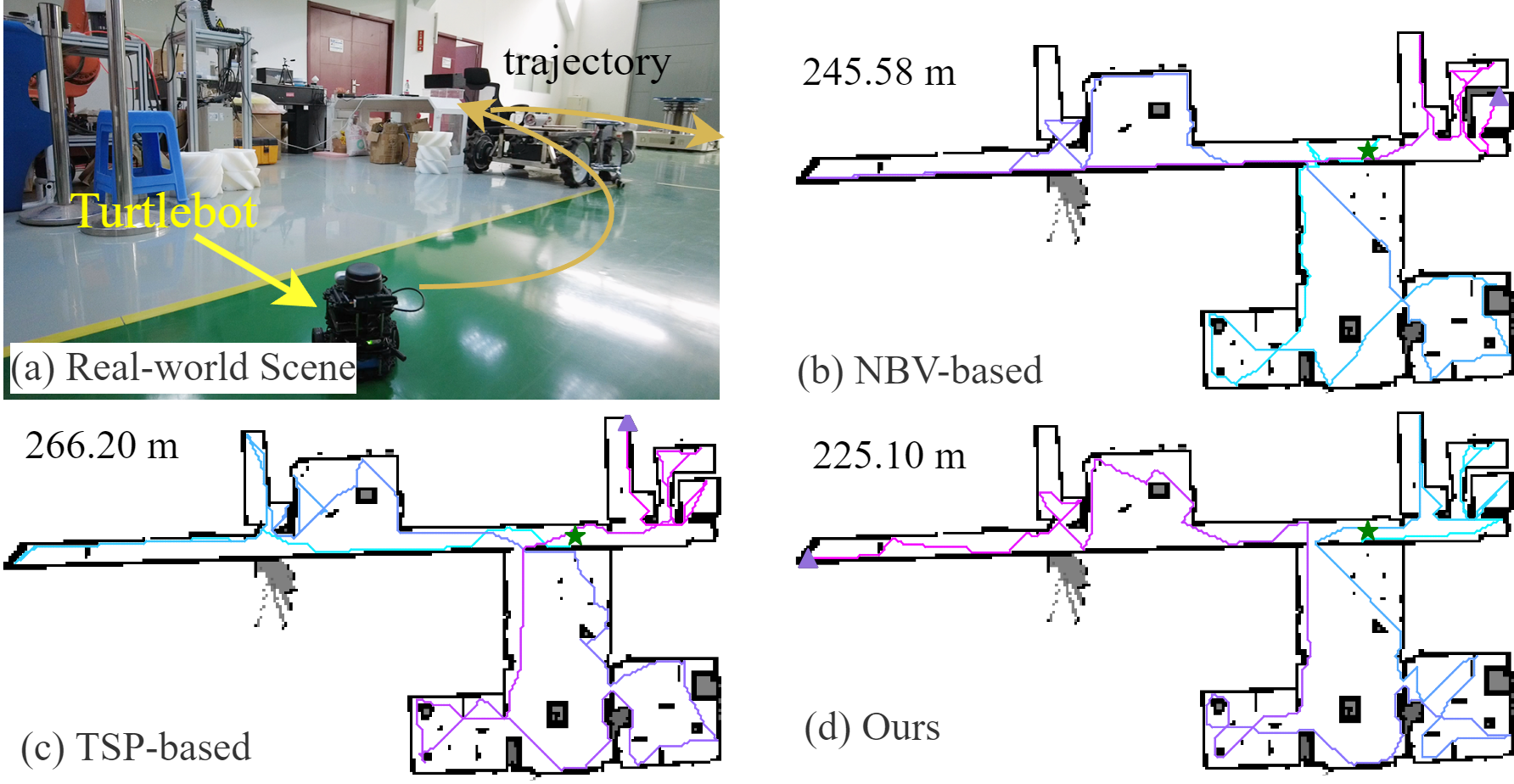
Figure 6: Illustration of the real-world experiment. (a) A screenshot captured of the robot in the real-world scene. (b) (c) (d) Results of different methods in the scene.

The result can be found in Fig. 6. The effectiveness of the proposed method is compared with NBV and TSP. The total path lengths of NBV and TSP are 245.58 m, and 266.20 m, respectively. By implementing map prediction in the process, the robot uses 225.10 m to finish the exploration. This result indicates that map prediction can exhibit a certain degree of generalization, even in previously unseen scenarios.

IV Conclusion & Future Work

In this work, we focus on facilitating the efficiency of exploration using map prediction in a clustered environment. Firstly, we perform floor plan extraction by denoising the cluttered map using UNet++. Then, we use a floor plan-based algorithm to improve the prediction ability. Additionally, we also abstract and extract the positions of rooms and their connectivity based on the predicted results. The effectiveness of the proposed method is demonstrated by exploration and navigation in unknown environments. In exploration, compared with the SOTA method, our method can shorten the path length by 7.93%. In navigation, the proposed method also achieves 24.85% improvement.

Currently, this paper only considers a simple method of applying predicted information to exploration tasks. In future work, more efficient utilization of predicted information through methods such as reinforcement learning is expected, which could further enhance exploration efficiency.

References

- [1] A. Padalkar, A. Pooley, A. Jain, A. Bewley, A. Herzog, A. Irpan, A. Khazatsky, A. Rai, A. Singh, A. Brohan, et al., “Open x-embodiment: Robotic learning datasets and rt-x models,” arXiv preprint arXiv:2310.08864, 2023.
- [2] D. Hoeller, N. Rudin, D. Sako, and M. Hutter, “Anymal parkour: Learning agile navigation for quadrupedal robots,” Sci. Robot., vol. 9, no. 88, p. eadi7566, 2024.
- [3] N. Yokoyama, S. Ha, D. Batra, J. Wang, and B. Bucher, “Vlfm: Vision-language frontier maps for zero-shot semantic navigation,” in Proc. IEEE Int. Conf. Robot. Autom., pp. 42–48, IEEE, 2024.
- [4] C. Cao, H. Zhu, Z. Ren, H. Choset, and J. Zhang, “Representation granularity enables time-efficient autonomous exploration in large, complex worlds,” Sci. Robot., vol. 8, no. 80, 2023.
- [5] B. Zhou, H. Xu, and S. Shen, “Racer: Rapid collaborative exploration with a decentralized multi-uav system,” IEEE Trans. Robotics, 2023.
- [6] T. Marcucci, M. Petersen, D. von Wrangel, and R. Tedrake, “Motion planning around obstacles with convex optimization,” Sci. Robot., vol. 8, no. 84, p. eadf7843, 2023.
- [7] G. Best, R. Garg, J. Keller, G. A. Hollinger, and S. Scherer, “Multi-robot, multi-sensor exploration of multifarious environments with full mission aerial autonomy,” Int. J. Robot. Res., vol. 43, no. 4, pp. 485–512, 2024.
- [8] Y. Tao, Y. Wu, B. Li, F. Cladera, A. Zhou, D. Thakur, and V. Kumar, “Seer: Safe efficient exploration for aerial robots using learning to predict information gain,” in Proc. IEEE Int. Conf. Robot. Autom., pp. 1235–1241, IEEE, 2023.
- [9] Y. Tao, E. Iceland, B. Li, E. Zwecher, U. Heinemann, A. Cohen, A. Avni, O. Gal, A. Barel, and V. Kumar, “Learning to explore indoor environments using autonomous micro aerial vehicles,” in Proc. IEEE Int. Conf. Robot. Autom., pp. 15758–15764, IEEE, 2024.
- [10] K. Katyal, K. Popek, C. Paxton, P. Burlina, and G. D. Hager, “Uncertainty-aware occupancy map prediction using generative networks for robot navigation,” in Proc. IEEE Int. Conf. Robot. Autom., pp. 5453–5459, IEEE, 2019.
- [11] A. Elhafsi, B. Ivanovic, L. Janson, and M. Pavone, “Map-predictive motion planning in unknown environments,” in Proc. IEEE Int. Conf. Robot. Autom., pp. 8552–8558, IEEE, 2020.
- [12] M. Wei, D. Lee, V. Isler, and D. Lee, “Occupancy map inpainting for online robot navigation,” in Proc. IEEE Int. Conf. Robot. Autom., pp. 8551–8557, IEEE, 2021.
- [13] G. Hardouin, J. Moras, F. Morbidi, J. Marzat, and E. M. Mouaddib, “A multirobot system for 3-d surface reconstruction with centralized and distributed architectures,” IEEE Trans. Robotics, 2023.
- [14] H. Umari and S. Mukhopadhyay, “Autonomous robotic exploration based on multiple rapidly-exploring randomized trees,” in Proc. IEEE/RSJ Int. Conf. Intell. Robot. Syst., pp. 1396–1402, 2017.
- [15] A. Patwardhan and A. J. Davison, “A distributed multi-robot framework for exploration, information acquisition and consensus,” in Proc. IEEE Int. Conf. Robot. Autom., pp. 12062–12068, IEEE, 2024.
- [16] A. Asgharivaskasi, F. Girke, and N. Atanasov, “Riemannian optimization for active mapping with robot teams,” arXiv preprint arXiv:2404.18321, 2024.
- [17] H. Choset, “Coverage of known spaces: The boustrophedon cellular decomposition,” Auton. Robot., vol. 9, pp. 247–253, 2000.
- [18] L. Ericson, D. Duberg, and P. Jensfelt, “Understanding greediness in map-predictive exploration planning,” in Eur. Conf. Mob. Robots, pp. 1–7, IEEE, 2021.
- [19] H. J. Chang, C. G. Lee, Y.-H. Lu, and Y. C. Hu, “P-slam: Simultaneous localization and mapping with environmental-structure prediction,” IEEE Trans. Robotics, vol. 23, no. 2, pp. 281–293, 2007.
- [20] M. Luperto, V. Arcerito, and F. Amigoni, “Predicting the layout of partially observed rooms from grid maps,” in Proc. IEEE Int. Conf. Robot. Autom., pp. 6898–6904, IEEE, 2019.
- [21] L. Ericson and P. Jensfelt, “Floorgent: Generative vector graphic model of floor plans for robotics,” in Proc. IEEE/RSJ Int. Conf. Intell. Robot. Syst., pp. 12485–12491, IEEE, 2022.
- [22] L. Ericson and P. Jensfelt, “Beyond the frontier: Predicting unseen walls from occupancy grids by learning from floor plans,” IEEE Robot. Automat. Lett., 2024.
- [23] K. D. Katyal, A. Polevoy, J. Moore, C. Knuth, and K. M. Popek, “High-speed robot navigation using predicted occupancy maps,” in Proc. IEEE Int. Conf. Robot. Autom., pp. 5476–5482, IEEE, 2021.
- [24] S. K. Ramakrishnan, Z. Al-Halah, and K. Grauman, “Occupancy anticipation for efficient exploration and navigation,” pp. 400–418, Springer, 2020.
- [25] L. Wang, H. Ye, Q. Wang, Y. Gao, C. Xu, and F. Gao, “Learning-based 3d occupancy prediction for autonomous navigation in occluded environments,” in Proc. IEEE/RSJ Int. Conf. Intell. Robot. Syst., pp. 4509–4516, IEEE, 2021.
- [26] V. D. Sharma, J. Chen, and P. Tokekar, “Proxmap: Proximal occupancy map prediction for efficient indoor robot navigation,” in Proc. IEEE/RSJ Int. Conf. Intell. Robot. Syst., pp. 7135–7140, IEEE, 2023.
- [27] Y. Ji, Z. Chen, E. Xie, L. Hong, X. Liu, Z. Liu, T. Lu, Z. Li, and P. Luo, “Ddp: Diffusion model for dense visual prediction,” in Proc. IEEE Int. Conf. Comp. Vis., pp. 21741–21752, 2023.
- [28] B. Chen, Y. Cui, P. Zhong, W. Yang, Y. Liang, and J. Wang, “Stexplorer: A hierarchical autonomous exploration strategy with spatio-temporal awareness for aerial robots,” ACM Trans. Intell. Syst. Technol., vol. 14, no. 6, pp. 1–24, 2023.
- [29] A. Aydemir, P. Jensfelt, and J. Folkesson, “What can we learn from 38,000 rooms? reasoning about unexplored space in indoor environments,” in Proc. IEEE/RSJ Int. Conf. Intell. Robot. Syst., pp. 4675–4682, IEEE, 2012.
- [30] Z. Zhou, M. M. Rahman Siddiquee, N. Tajbakhsh, and J. Liang, “Unet++: A nested u-net architecture for medical image segmentation,” in Proc. Int. Conf. Med. Image Comput. Comput.-Assist. Interv., pp. 3–11, Springer, 2018.
- [31] O. Ronneberger, P. Fischer, and T. Brox, “U-net: Convolutional networks for biomedical image segmentation,” in Proc. 18th Int. Conf. Med. Image Comput. Comput.-Assist. Interv., pp. 234–241, Springer, 2015.
- [32] S. Kim, M. Corah, J. Keller, G. Best, and S. Scherer, “Multi-robot multi-room exploration with geometric cue extraction and circular decomposition,” IEEE Robot. Automat. Lett., 2023.