A modified recursive transfer matrix algorithm for radiation and scattering computation of multilayer spheres

Abstract

We discusses the electromagnetic scattering and radiation problems of multilayered spheres, reviewing the historical expansion of the Lorentz-Mie theory and the numerical stability issues encountered in handling multilayered spheres. By combining recursive methods with the transfer matrix method, we propose a modified transfer matrix algorithm designed for the stable and efficient calculation of electromagnetic scattering coefficients of multilayered spheres. The new algorithm simplifies the recursive formulas by introducing Debye potentials and logarithmic derivatives, effectively avoiding numerical overflow issues associated with Bessel functions under large complex variables. Numerical test results demonstrate that this algorithm offers superior stability and applicability when dealing with complex cases such as thin shells and strongly absorbing media.

Keywords transfer matrix  $\cdot$ recursive algorithm  $\cdot$ multilayer sphere  $\cdot$ Bessel functions

1 Introduction

The problem of electromagnetic wave scattering by spherical particles was first proposed and addressed by Mie, Lorentz, and Debye, and is commonly known as the Lorentz-Mie theory or the Lorentz-Mie-Debye theory. For over a century, this theory has been an important topic of research in various fields such as electromagnetism[1], optics[2], thermal and statistical physics[3, 4]. Numerous monographs and papers have discussed this problem. On the other hand, the thermal fluctuations of electromagnetic waves are a core issue in radiative transfer, explaining groundbreaking discoveries such as Planck’s law of blackbody radiation, proposed nearly a century ago. Electromagnetic thermal radiation itself can also be concisely expressed using the scattering operator of an object. The study of electromagnetic scattering and radiation of (multilayered) spheres is of fundamental importance for research in physical theory and has practical significance in applications such as remote sensing and imaging, biomedicine, photovoltaic design, and optical antennas.

As early as 1951, Aden and Kerker[5] extended the Lorentz-Mie theory to the case of coated spheres. For multilayered spheres, the electric and magnetic fields are represented as multipole expansions, with the coefficients of these expansions determined by the boundary conditions at the interfaces of the sphere’s layers. Kerker[6] further extended this theory to multilayered spheres. In the early days, applying Kerker’s formulas to calculate the scattering of multilayered spheres often encountered various numerical issues, partly due to the use of incorrect recurrence formulas for calculating Bessel functions. Even with correct recurrence formulas, numerical problems still arose when calculating thin-shell spheres, strongly absorbing media, and highly multilayered cases. To address these numerical stability issues, Toon and Ackerman[7] reformulated Kerker’s equations using logarithmic derivatives, providing a stable algorithm for scattering by double-layered spheres. Further, Wu and Wang[8] proposed a concise recursive method to calculate electromagnetic scattering coefficients for arbitrary multilayered spheres. Johnson[9] also developed a slightly different recurrence algorithm. However, numerical errors persisted when dealing with thin, strongly absorbing shells. Kaiser and Schweiger[10] proposed a numerically stable algorithm for calculating Mie scattering coefficients of coated spheres, but it could not be easily extended to arbitrary multilayered spheres. Building on the work of Wu and Wang, Yang[11] proposed an improved recursive algorithm for stable calculations of Mie scattering coefficients in complex cases, such as multilayered and strongly absorbing media. In the field of electromagnetics, Chew[1] developed a layered medium framework suitable for spherical cases, which resulted in concise recurrence formulas. Recently, Yuan et al.[12] introduced these ideas into the spherical layered medium framework, yielding a set of numerically stable calculation schemes. In mathematical physics, Moroz[13] proposed the transfer matrix method for solving the electromagnetic wave scattering problem of multilayered spheres. The transfer matrix method is an important and highly efficient technique for solving general scattering problems, although it still has some limitations in terms of applicability[14, 15].

To expand its applicability, this paper discusses an improved transfer matrix algorithm for the efficient and stable calculation of electromagnetic scattering and radiation by multilayered spheres. Our derivation of the spherical transfer matrix differs slightly from Moroz’s approach, as we use Debye potentials to simplify the expressions, providing a new recursive format and a numerically stable algorithm that avoids overflow issues. Section 2 introduces the transfer matrix method for electromagnetic wave scattering by multilayered spheres and presents new recursive formulas. Section 3 demonstrates a stable calculation scheme for the recursive formulas obtained through logarithmic derivatives or ratios of Bessel functions, with the final algorithm effectively avoiding round-off errors and numerical overflow issues caused by the imaginary part of large complex variables. Section 4 discusses three numerical test cases, showcasing the stability and applicability of the proposed algorithm. Section 5 concludes with a summary of the algorithm and results.

2 Theory

In spherical coordinates, the complete electromagnetic fields can be expressed using two scalar functions (Debye potential). The Deybe potentials $\pi_{m}$ and $\pi_{e}$ satisfy the scalar Helmholtz equation,

$$(\nabla^{2}+k^{2})\pi_{e/m}=0$$ (1)

with the wavenumber $k=\sqrt{\omega^{2}\epsilon(r)\mu(r)}$, $\omega$ is the vacuum wavelength, and $\epsilon$ and $\mu$ represent the permittivity and permeability of the medium, respectively.

Due to spherical symmetry of multilayered spheres (see Figure 1), Debye potentials can be expanded as a sum of discrete modes $R_{l}(r)P^{m}_{l}(\cos\theta)\exp(im\phi)$. $\epsilon(r)$ and $\mu(r)$ are constant within each spherical layer, the general form of the radial function $R_{l}(r)$ within each layer is a linear combination of spherical Bessel functions:

$$R_{l}(r)\big{|}_{i}=A_{i}j_{l}(k_{i}r)+B_{i}h^{(1)}_{l}(k_{i}r)$$ (2)

where $j_{l}(z)$ and $h^{(1)}_{l}(z)$ are the spherical Bessel functions of the first and third kind, respectively. The expansion system of the scattered electromagnetic field, however, is composed of the corresponding Riccati-Bessel functions:

$$\psi_{l}(z)=zj_{l}(z),\qquad\xi_{l}(z)=zh^{(1)}_{l}(z)$$

The coefficient vectors $c_{i}^{T}=(A_{i},B_{i})^{T}$ for adjacent spherical layers are related by the boundary conditions at the interface, where the tangential components of the electromagnetic fields are continuous. Then, the boundary conditions at $r=r_{i}$ lead to

$$\Lambda^{\sigma}_{i+1}\Phi_{i+1}c_{i+1}=\Lambda^{\sigma}_{i}\Phi_{i}c_{i}$$ (3)

where $\sigma=m/e$ denotes polarization, the fundamental matrix $\Phi_{i}$ is given by

$$\Phi_{i}(r)=\begin{pmatrix}\psi_{l}(k_{i}r)&\xi_{l}(k_{i}r)\\ \psi^{\prime}_{l}(k_{i}r)&\xi^{\prime}_{l}(k_{i}r)\end{pmatrix}$$ (4)

Its inverse matrix is given by

$$\Phi_{i}^{-1}(r)=\frac{1}{w_{l}(k_{i}r)}\begin{pmatrix}\xi^{\prime}_{l}(k_{i}r)&-\xi_{l}(k_{i}r)\\ -\psi^{\prime}_{l}(k_{i}r)&\psi_{l}(k_{i}r)\end{pmatrix}$$ (5)

with the Wronskian,

$$w_{l}(k_{i}r)=\psi_{l}(k_{i}r)\xi^{\prime}_{l}(k_{i}r)-\xi_{l}(k_{i}r)\psi^{\prime}_{l}(k_{i}r)$$ (6)

Furthermore, $\Lambda^{\sigma}_{i}$ is a diagonal matrix, and its specific form depends on the convention. For transverse magnetic (TM) polarization,

$$\Lambda^{m}_{i}=\begin{pmatrix}\frac{\epsilon_{i}}{k_{i}}&0\\ 0&1\end{pmatrix}$$ (7)

The transverse electric (TE) $\Lambda^{e}_{i}$ can be obtained by the duality principle. The matrix $\Lambda^{\sigma}_{i}$ acts as a scaling factor. For the sake of simplicity in the derivation, we can incorporate it into the fundamental matrix, such as $\frac{\epsilon_{i}}{k_{i}}\psi_{l}(k_{i}r_{i})\to\tilde{\psi}_{l}(k_{i}r_{i})$. Without affecting understanding, we omit the superscript $\tilde{\cdot}$ and eventually restore the final expression. Multiplying both sides of the equation by $\Phi^{-1}_{i+1}$, we get

$$\begin{pmatrix}A_{i+1}\\ B_{i+1}\end{pmatrix}=M_{i+1,i}\begin{pmatrix}A_{i}\\ B_{i}\end{pmatrix}$$ (8)

where the matrix $M_{i+1,i}$ connects the coefficients of adjacent layers and is called the transfer matrix.

$$M_{i+1,i} = \Phi_{i+1}^{-1}\Phi_{i}$$

$$= \frac{1}{w_{l}(z^{+}_{i})}\begin{pmatrix}\psi_{l}(z_{i})\xi^{\prime}_{l}(z^{+}_{i})-\psi^{\prime}_{l}(z_{i})\xi_{l}(z^{+}_{i})&\xi^{\prime}_{l}(z^{+}_{i})\xi_{l}(z_{i})-\xi_{l}(z^{+}_{i})\xi^{\prime}_{l}(z_{i})\\ -\psi_{l}(z_{i})\psi^{\prime}_{l}(z^{+}_{i})+\psi^{\prime}_{l}(z_{i})\psi_{l}(z^{+}_{i})&-\psi^{\prime}_{l}(k_{i+1}r_{i})\xi_{l}(z_{i})+\psi_{l}(z^{+}_{i})\xi^{\prime}_{l}(z_{i})\end{pmatrix}$$

with $z_{i}=k_{i}r_{i}$, $z^{+}_{i}=k_{i+1}r_{i}$. For an $n$-layered sphere, we have the following formula

$$\begin{pmatrix}A_{n+1}\\ B_{n+1}\end{pmatrix}=M_{n+1,n}M_{n,n-1}...M_{3,2}M_{2,1}\begin{pmatrix}A_{1}\\ B_{1}\end{pmatrix}=M\begin{pmatrix}A_{1}\\ B_{1}\end{pmatrix}$$ (9)

Since the third kind of Bessel functions are singular at the origin, we set $A_{1}=1$ and $B_{1}=0$. Therefore, the coefficients in the outermost medium are directly given by elements of $M$, i.e., $A_{n+1}=M_{11}$ and $B_{n+1}=M_{21}$. The total scattering coefficients for the $n$-layered sphere are given by the following formula:

$$\mathcal{T}_{\sigma,l}=\frac{B_{n+1}}{A_{n+1}}=\frac{M_{11}}{M_{21}}$$ (10)

Due to the spherical symmetry, the T matrix of the multilayered sphere is diagonal, and its diagonal elements correspond exactly to the Mie scattering coefficients.

$$\mathcal{T}_{\mu\mu^{\prime}}=\mathcal{T}_{\sigma,l}\delta_{\sigma\sigma^{\prime}}\delta_{l,l^{\prime}}\delta_{mm^{\prime}}$$

$\mu=\{\sigma,l,m\}$ is the index of the supermatrix. By summing over all TM and TE polarizations and channel contributions, the scattering and extinction efficiencies are determined by:

$$Q_{sca}=\frac{2}{x^{2}}\text{Tr}\Big{(}\mathcal{T}^{\dagger}\mathcal{T}\Big{)}$$ (11)

$$Q_{ext}=-\frac{2}{x^{2}}\text{Tr}\Big{(}\frac{\mathcal{T}^{\dagger}+\mathcal{T}}{2}\Big{)}$$ (12)

Here, $x=2\pi R/\lambda$ is the size parameter, where $R$ is the radius of the outermost layer of the sphere, and $\lambda$ is the wavelength in vacuum. The absorption efficiency is given by $Q_{abs}=Q_{ext}-Q_{sca}$. The above expression is also applicable to irregularly shaped objects, such as those discussed in our previous work[16] on scattering from randomly shaped geometries. The energy emissivity of the multilayered sphere is given by the following formula[4, 17]:

$$H_{s} = \frac{8\pi^{2}R^{2}hc^{2}}{\lambda^{5}}\int^{\infty}_{0}d\lambda\frac{1}{\exp{\frac{hc}{k_{B}T\lambda}}-1}Q_{abs}$$ (13)

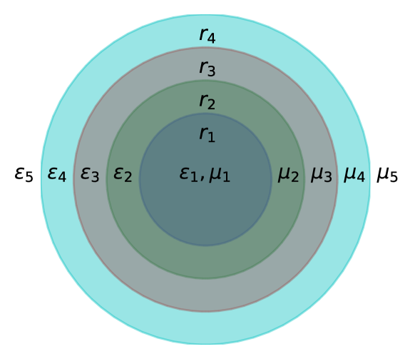
Figure 1: Schematic of an n-layer sphere embedded in an infinite dielectric medium. The outer radius, permittivity, and permeability of each layer are $r_{i}{\hskip 0.0pt},\epsilon_{i}{\hskip 0.0pt}$, and $\mu_{i}$, respectively, where $i=1,2,…,n$. The permittivity of the medium is the permittivity in vacuum $\epsilon_{n+1}{\hskip 0.0pt}=\epsilon_{0}$.

Here, $k_{B}$ and $h$ are the Boltzmann and Planck constants, respectively, and $c$ is the speed of light in vacuum.

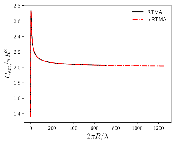
Figure 2: The extinction efficiency $Q_{ext}$of the coated sphere as a function of the outermost layer’s size parameter is shown. The plot compares the results with those obtained using RTMA. The refractive indices of the core and shell are $m_{1}=1.33+i0.00$ and $m_{2}=1.33+i$i, respectively.

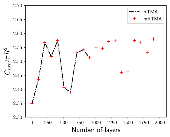
Figure 3: The extinction efficiency $Q_{ext}$ of the multilayer sphere as a function of the number of layers is shown. The plot compares the results with those obtained using RTMA. The refractive index of each layer is randomly generated.

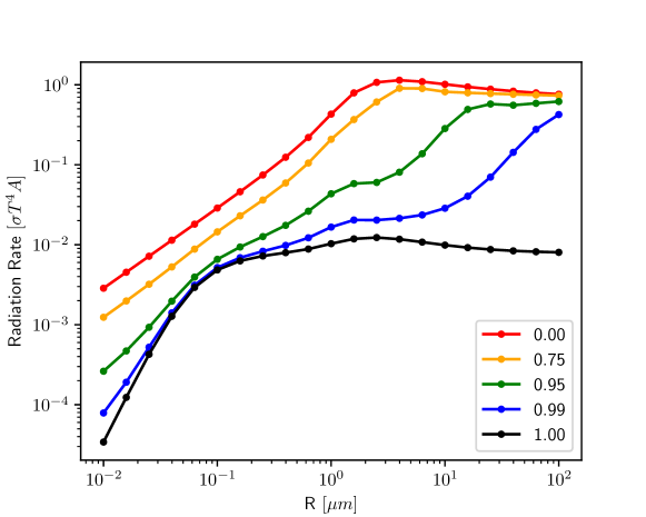
Figure 4: The emitted energy of a SiC+gold coated sphere at a temperature of 300K, as a function of the outer radius R, is normalized with respect to the Stefan-Boltzmann result. Different curves correspond to different ratios of inner to outer layer radii.

3 Algorithm

Next, we derive the recursive algorithm. The scattering coefficient for each layer can be given by the following equation:

$$\mathcal{T}^{i}_{\sigma,l}=\frac{B_{i}}{A_{i}}$$

Additionally, we obtain a set of recursive equations:

$$\mathcal{T}^{i+1}_{\sigma,l}=\frac{M^{21}_{i+1,i}+M^{22}_{i+1,i}\mathcal{T}^{i}_{\sigma,l}}{M^{11}_{i+1,i}+M^{12}_{i+1,i}\mathcal{T}^{i}_{\sigma,l}}$$ (14)

Substituting the elements of the transfer matrix into the above expression, we have:

$$\mathcal{T}^{i+1}_{\sigma,l}=\frac{\psi^{\prime}_{l}(z_{i})\psi_{l}(z^{+}_{i})-\psi_{l}(z_{i})\psi^{\prime}_{l}(z^{+}_{i})+(\psi_{l}(z^{+}_{i})\xi^{\prime}_{l}(z_{i})-\psi^{\prime}_{l}(z^{+}_{i})\xi_{l}(z_{i}))\mathcal{T}^{i}_{\sigma,l}}{\psi_{l}(z_{i})\xi^{\prime}_{l}(z^{+}_{i})-\psi^{\prime}_{l}(z_{i})\xi_{l}(z^{+}_{i})+(\xi_{l}(z_{i})\xi^{\prime}_{l}(z^{+}_{i})-\xi^{\prime}_{l}(z_{i})\xi_{l}(z^{+}_{i}))\mathcal{T}^{i}_{\sigma,l}}$$ (15)

When the refractive index of the sphere is real, the arguments of the Bessel function and its derivative are also real, making it easy to obtain robust recurrence formulas for their evaluation. However, when the refractive index is complex, the calculation of the Bessel function becomes unstable as it enters the exponential domain and goes out of bounds. To avoid this ill-conditioning, the calculation formula will involve only the ratios and logarithmic derivatives of the Bessel functions. The logarithmic derivatives are

$$D_{l}(z)=\frac{\psi^{\prime}_{l}(z)}{\psi_{l}(z)},\qquad F_{l}(z)=\frac{\xi^{\prime}_{l}(z)}{\xi_{n}(z)}$$ (16)

For the case of a multilayer sphere, $\mathcal{T}^{i}_{\sigma,l}$ may still encounter numerical overflow issue. To avoid this issue, we define a rescaled scattering coefficient $\tilde{\mathcal{T}}^{i}_{\sigma,l}$ and a combined ratio $Q^{i}_{l}$ [11]

$$\tilde{\mathcal{T}}^{i}_{\sigma,l}=\frac{\xi_{l}(z^{+}_{i-1})}{\psi_{l}(z^{+}_{i-1})}\mathcal{T}^{i}_{\sigma,l},\qquad Q^{i}_{l}=\frac{\psi_{l}(z^{+}_{i-1})\xi_{l}(z_{i})}{\psi_{l}(z_{i})\xi_{l}(z^{+}_{i-1})}$$

Then, the recurrence formula becomes

$$\tilde{\mathcal{T}}^{i+1}_{\sigma,l}=-\frac{\big{(}D_{l}(z^{+}_{i})-D_{l}(z_{i})\big{)}+Q^{i}_{l}\big{(}D_{l}(z^{+}_{i})-F_{l}(z_{i})\big{)}\tilde{\mathcal{T}}^{i}_{\sigma,l}}{\big{(}F_{l}(z^{+}_{i})-D_{l}(z_{i})\big{)}+Q^{i}_{l}\big{(}F_{l}(z^{+}_{i})-F_{l}(z_{i})\big{)}\tilde{\mathcal{T}}^{i}_{\sigma,l}}$$ (17)

with

$$\tilde{\mathcal{T}}^{0}_{\sigma,l}=0$$

Consequently, we can recover the formula for TM wave,

$$\tilde{\mathcal{T}}^{i+1}_{m,l}=-\frac{\big{(}\sqrt{\epsilon_{i}\mu_{i+1}}D_{l}(z^{+}_{i})-\sqrt{\epsilon_{i+1}\mu_{i}}D_{l}(z_{i})\big{)}+Q^{i}_{l}\big{(}\sqrt{\epsilon_{i}\mu_{i+1}}D_{l}(z^{+}_{i})-\sqrt{\epsilon_{i+1}\mu_{i}}F_{l}(z_{i})\big{)}\tilde{\mathcal{T}}^{i}_{m,l}}{\big{(}\sqrt{\epsilon_{i}\mu_{i+1}}F_{l}(z^{+}_{i})-\sqrt{\epsilon_{i+1}\mu_{i}}D_{l}(z_{i})\big{)}+Q^{i}_{l}\big{(}\sqrt{\epsilon_{i}\mu_{i+1}}F_{l}(z^{+}_{i})-\sqrt{\epsilon_{i+1}\mu_{i}}F_{l}(z_{i})\big{)}\tilde{\mathcal{T}}^{i}_{m,l}}$$

By duality, then

$$\tilde{\mathcal{T}}^{i+1}_{e,l}=-\frac{\big{(}\sqrt{\epsilon_{i+1}\mu_{i}}D_{l}(z^{+}_{i})-\sqrt{\epsilon_{i}\mu_{i+1}}D_{l}(z_{i})\big{)}+Q^{i}_{l}\big{(}\sqrt{\epsilon_{i+1}\mu_{i}}D_{l}(z^{+}_{i})-\sqrt{\epsilon_{i}\mu_{i+1}}F_{l}(z_{i})\big{)}\tilde{\mathcal{T}}^{i}_{e,l}}{\big{(}\sqrt{\epsilon_{i+1}\mu_{i}}F_{l}(z^{+}_{i})-\sqrt{\epsilon_{i}\mu_{i+1}}D_{l}(z_{i})\big{)}+Q^{i}_{l}\big{(}\sqrt{\epsilon_{i+1}\mu_{i}}F_{l}(z^{+}_{i})-\sqrt{\epsilon_{i}\mu_{i+1}}F_{l}(z_{i})\big{)}\tilde{\mathcal{T}}^{i}_{e,l}}$$

In addition to the above standing wave case, we can also consider the outgoing waves case[1]. Similarly, we define

$$\tilde{\mathcal{T}}^{i}_{\sigma,l}=\frac{\psi_{l}(z_{i})}{\xi_{l}(z_{i})}\mathcal{T}^{i}_{\sigma,l}$$

Then, it is easy to obtain the rescaled Mie scattering coefficient for the outgoing wave case,

$$\tilde{\mathcal{T}}^{i}_{\sigma,l} = -\frac{\big{(}F_{l}(z^{+}_{i})-F_{l}(z_{i})\big{)}+Q^{i+1}_{l}\big{(}D_{l}(z^{+}_{i})-D_{l}(z_{i})\big{)}\tilde{\mathcal{T}}^{i+1}_{\sigma,l}}{\big{(}F_{l}(z^{+}_{i})-D_{l}(z_{i})\big{)}+Q^{i+1}_{l}\big{(}D_{l}(z^{+}_{i})-D_{l}(z_{i})\big{)}\tilde{\mathcal{T}}^{i+1}_{\sigma,l}}$$ (18)

Consequently, we can recover the formula for TM wave,

$$\tilde{\mathcal{T}}^{i}_{m,l} = -\frac{\big{(}\sqrt{\epsilon_{i}\mu_{i+1}}F_{l}(z^{+}_{i})-\sqrt{\epsilon_{i+1}\mu_{i}}F_{l}(z_{i})\big{)}+Q^{i+1}_{l}\big{(}\sqrt{\epsilon_{i}\mu_{i+1}}D_{l}(z^{+}_{i})-\sqrt{\epsilon_{i+1}\mu_{i}}D_{l}(z_{i})\big{)}\tilde{\mathcal{T}}^{i+1}_{m,l}}{\big{(}\sqrt{\epsilon_{i}\mu_{i+1}}F_{l}(z^{+}_{i})-\sqrt{\epsilon_{i+1}\mu_{i}}D_{l}(z_{i})\big{)}+Q^{i+1}_{l}\big{(}\sqrt{\epsilon_{i}\mu_{i+1}}D_{l}(z^{+}_{i})-\sqrt{\epsilon_{i+1}\mu_{i}}D_{l}(z_{i})\big{)}\tilde{\mathcal{T}}^{i+1}_{m,l}}$$

By duality, then

$$\tilde{\mathcal{T}}^{i}_{e,l} = -\frac{\big{(}\sqrt{\epsilon_{i+1}\mu_{i}}F_{l}(z^{+}_{i})-\sqrt{\epsilon_{i}\mu_{i+1}}F_{l}(z_{i})\big{)}+Q^{i+1}_{l}\big{(}\sqrt{\epsilon_{i+1}\mu_{i}}D_{l}(z^{+}_{i})-\sqrt{\epsilon_{i}\mu_{i+1}}D_{l}(z_{i})\big{)}\tilde{\mathcal{T}}^{i+1}_{e,l}}{\big{(}\sqrt{\epsilon_{i+1}\mu_{i}}F_{l}(z^{+}_{i})-\sqrt{\epsilon_{i}\mu_{i+1}}D_{l}(z_{i})\big{)}+Q^{i+1}_{l}\big{(}\sqrt{\epsilon_{i+1}\mu_{i}}D_{l}(z^{+}_{i})-\sqrt{\epsilon_{i}\mu_{i+1}}D_{l}(z_{i})\big{)}\tilde{\mathcal{T}}^{i+1}_{e,l}}$$

The downward recursion for $D_{l}$ is numerically stable. Therefore, we use the following recursive formula for computation[18]:

$$D_{l-1}(z) = \frac{l}{z}-\Big{(}\frac{l}{z}+D_{l}(z)\Big{)}^{-1}$$ (19)

The upward recursion for $F_{l}$ is numerically stable. Therefore, we use the following recursive formula for computation:

$$F_{l}(z) = \Big{(}\frac{l}{z}-F_{l-1}(z)\Big{)}^{-1}-\frac{l}{z}$$ (20)

Using logarithmic derivatives, Toon and Ackerman[7] provided a stable recursive algorithm for the ratio of Bessel functions $\frac{\psi_{l}(z^{+}_{i-1})}{\psi_{l}(z_{i})}$. Similarly, the ratio $\frac{\xi_{l}(z_{i})}{\xi_{l}(z^{+}_{i-1})}$ can be computed using a similar approach. Yang[11] combined these two ratios into a single calculation.

$$Q^{i}_{l}=\frac{D_{l}(z_{i})+l/z_{i}}{D_{l}(z^{+}_{i-1})+l/z^{+}_{i-1}}\frac{F_{l}(z^{+}_{i-1})+l/z^{+}_{i-1}}{F_{l}(z_{i})+l/z_{i}}Q^{i}_{l-1}$$ (21)

with initial values,

$$Q^{i}_{0}=e^{-2(\text{Im}z^{+}_{i-1}-\text{Im}z_{i})}\frac{e^{-2\text{Re}z^{+}_{i-1}}-e^{-2\text{Im}z^{+}_{i-1}}}{e^{-2\text{Re}z_{i}}-e^{-2\text{Im}z_{i}}}$$ (22)

The main contribution of this paper is the improvement of the transfer matrix method, making it suitable for recursive computation, which can be applied to cases with an ultra-high number of layers and strongly absorbing media. Compared to the work of Wu, Yang, and others, our recursive formulas are more concise and allow for the sequential computation of expansion coefficients for each spherical layer, making the algorithm more efficient. Additionally, we have derived recursive formulas applicable to the outgoing wave scenario.

Bessel functions are frequently used in the analysis of scattering and radiation problems involving electromagnetic waves, acoustic waves, and other phenomena. Numerous studies have been conducted on the precise computation of spherical Bessel functions. Classical algorithms include Miller’s algorithm[19], which utilizes a simple backward recurrence relation, Gautschi’s algorithm[20], and Olver’s algorithm[21], which can automatically estimate truncation errors. These algorithms are capable of computing a class of special functions, including Bessel functions. Some methods[22, 23] for computing Bessel functions are special cases of the aforementioned algorithms. As an auxiliary work, this paper extends a previously proposed stable algorithm [24] for computing Bessel functions to allow the computation of general second-order difference equations. For a general three-term recurrence difference equation, the expression is given by:

$$a_{n}\psi_{n-1}+b_{n}\psi_{n}+c_{n}\psi_{n+1}=d_{n}$$ (23)

As pointed out by[24], Miller’s algorithm and Gautschi’s algorithm are mathematically equivalent to $LU$ decomposition, while Olver’s algorithm is mathematically equivalent to $UL$ decomposition. We propose a new recursive algorithm based on $LDM^{T}$ decomposition, where $L$, $M^{T}$ and $D$ are lower triangular, upper triangular and diagonal matrices, respectively. Introduce the auxiliary variables, $\gamma_{n}$

$$\gamma_{n} = \Big{(}b_{n}-\gamma_{n-1}a_{n}c_{n-1}\Big{)}^{-1}$$ (24)

with $\gamma_{0}=0$. The forward and backward substitution algorithms are,

$$u_{1}=\gamma_{1}d_{1},\qquad u_{n}=\gamma_{n}(d_{n}-a_{n}u_{n-1})$$ (25)

and

$$\psi_{\nu}=u_{\nu},\qquad\psi_{n} = u_{n}-\gamma_{n}c_{n}\psi_{n+1}$$ (26)

with $\nu$ is the truncation order. The main advantage of this algorithm is that the truncation error could be estimated automatically. To estimate the optimal value of $\nu$, we increase the truncation order from $\nu$ to $\nu+1$. Thus, we obtain the following expression:

$$\psi^{(\nu+1)}_{n}-\psi^{(\nu)}_{n} = -\gamma_{n}c_{n}(\psi^{(\nu+1)}_{n+1}-\psi^{(\nu)}_{n+1})$$ (27)

$$= (-\gamma_{n}c_{n})(-\gamma_{n+1}c_{n+1})\cdots(-\gamma_{\nu-1}c_{\nu-1})(\psi^{(\nu+1)}_{\nu}-\psi^{(\nu)}_{\nu})$$

and

$$\psi^{(\nu+1)}_{\nu}-\psi^{(\nu)}_{\nu}=u_{\nu}-\gamma_{\nu}c_{\nu}\psi^{(\nu+1)}_{\nu+1}-u_{\nu}=-\gamma_{\nu}c_{\nu}u_{\nu+1}.$$ (28)

that is,

$$\psi^{(\nu+1)}_{n}-\psi^{(\nu)}_{n}=u_{\nu+1}\prod^{\nu}_{i=n}(-\gamma_{i}c_{i})$$ (29)

Let the truncated order be the smallest integer that satisfies the following inequality.

$$\Big{|}u_{\nu+1}\prod^{\nu}_{i=n}(-\gamma_{i}c_{i})\Big{|}<\frac{1}{2}\times 10^{-D}$$ (30)

The Bessel function $\psi_{n}$ can be computed to a precision of $D$ decimal digits, where $D$ is determined as the truncation criterion for the computational algorithm. The truncation error can be estimated with,

$$\epsilon^{(\nu)}=\psi_{n}-\psi^{(\nu)}_{n}=\sum^{\infty}_{s=\nu}u_{s+1}\prod^{s}_{i=n}(-\gamma_{i}c_{i})$$ (31)

For the computation of spherical Bessel functions, $a_{n}=c_{n}=1,b_{n}=-(2n+1)/z,d_{n}=0$. In this case, the factorization $LDM^{T}$ simplifies considerably since the underlying matrix is symmetric with $M=L$. This yields the $LDL^{T}$ factorization. With respect to the $LU$ factorization, the computational cost decreases to one half.

4 Results

The following section presents three test cases using the algorithm proposed in this paper. The first test case examines the scattering problem of a double-layered sphere with varying radii, where the refractive indices of the inner and outer layers are specified and compared with the RTMA. The second test case involves scattering by a multilayered sphere with the same radius, where the refractive indices of each shell are randomly generated, and the extinction cross-section is calculated for spheres with various numbers of layers. The third test case addresses the thermal radiation problem of a multilayered sphere, calculating the emissivity of a double-layered sphere.

In the first test, a coated sphere is considered, with the refractive indices of the core and shell layers set to $m_{1}=1.33+i0.0$ and $m_{2}=1.33+i$, respectively, and the core radius accounting for 50% of the total radius. The extinction efficiency $Q_{ext}$ is calculated for size parameters $x\in[1.0,1200.0]$. The RTMA experiences numerical overflow for $x>700.0$, while the mRTMA remains stable, as shown in Figure 2.

In the second test, we examined the scattering of a multilayered sphere with randomly generated refractive indices, with the total number of layers ranging from 2 to 2000. The refractive indices are generated as $n=n^{\prime}+in^{\prime\prime}$, with $n^{\prime}\sim\mathcal{U}_{[1,2]}$ and $\log_{10}n^{\prime\prime}\sim\mathcal{U}_{[-3,1]}$, where $\mathcal{U}$ denotes a uniform distribution. As shown in Figure 3, the mRTMA demonstrates significant improvement over the RTMA.

In the third test, the mRTMA is used to calculate the electromagnetic radiation of a double-layered sphere with varying radii, with the sphere maintained at a temperature of 300K in a cold environment. Figure 4 shows the radiation characteristics of the double-layered sphere, using SiC and gold as example materials, representing a dielectric and a conductor, respectively.

5 Conclusion

This paper reviews the Lorentz-Mie theory and its development in the context of electromagnetic scattering by multilayered spheres. It explores the numerical stability issues associated with multilayered sphere scattering and traces the evolution of various improved algorithms. By summarizing and comparing different recursive methods and transfer matrix algorithms, we identify the limitations and potential issues of these approaches, particularly when dealing with multilayered spheres, thin shells, and strongly absorbing media. Building on these earlier works, we propose an efficient recursive transfer matrix algorithm, demonstrating that it achieves high accuracy over a broad range of size parameters and significantly extends the applicability compared to the classical transfer matrix methods. Additionally, we propose and extend an algorithm for calculating spherical Bessel functions. Future work can focus on optimizing these numerical methods to further enhance their stability and applicability, providing more effective tools for solving complex electromagnetic scattering problems.

References

• [1] W. C. Chew. Waves and Fields in Inhomogenous Media. Wiley-IEEE Press, 1995.
• [2] C. F. Bohren and D. R. Huffman. Absorption and Scattering of Light by Small Particles. John Wiley&Songs, New York, 1983.
• [3] A. Narayanaswamy and G. Chen. Thermal near-field radiative transfer between two spheres. Phys. Rev. B, 77:075125, Feb 2008.
• [4] M. Krüger, G. Bimonte, T. Emig, and M. Kardar. Trace formulas for nonequilibrium casimir interactions, heat radiation, and heat transfer for arbitrary objects. Phys. Rev. B, 86:115423, Sep 2012.
• [5] A. L. Aden and M. Kerker. Scattering of Electromagnetic Waves from Two Concentric Spheres. Journal of Applied Physics, 22(10):1242–1246, 10 1951.
• [6] M. Kerker. The Scattering of Light and Other Electromagnetic Radiation. Academic, New York, 1969.
• [7] O. B. Toon and T. P. Ackerman. Algorithms for the calculation of scattering by stratified spheres. Appl. Opt., 20(20):3657–3660, Oct 1981.
• [8] Z. S. Wu and Y. P. Wang. Electromagnetic scattering for multilayered sphere: Recursive algorithms. Radio Science, 26(6):1393–1401, 1991.
• [9] B. R. Johnson. Light scattering by a multilayer sphere. Appl. Opt., 35(18):3286–3296, Jun 1996.
• [10] T. Kaiser and G. Schweiger. Stable algorithm for the computation of Mie coefficients for scattered and transmitted fields of a coated sphere. Computer in Physics, 7(6):682–686, 11 1993.
• [11] W. Yang. Improved recursive algorithm for light scattering by a multilayered sphere. Appl. Opt., 42(9):1710–1720, Mar 2003.
• [12] H. Yuan, W. Zhu, and B. O. Zhu. Numerically stable calculations of the spherically layered media theory. IEEE Transactions on Antennas and Propagation, 71(6):5178–5188, 2023.
• [13] A. Moroz. A recursive transfer-matrix solution for a dipole radiating inside and outside a stratified sphere. Annals of Physics, 315(2):352–418, 2005.
• [14] O. Peña and U. Pal. Scattering of electromagnetic radiation by a multilayered sphere. Computer Physics Communications, 180(11):2348–2354, 2009.
• [15] I. L. Rasskazov, P. S. Carney, and A. Moroz. Stratify: a comprehensive and versatile matlab code for a multilayered sphere. OSA Continuum, 3(8):2290–2306, Aug 2020.
• [16] J. Zhang, L. Bi, J. Liu, R. L. Panetta, P. Yang, and G. W. Kattawar. Optical scattering simulation of ice particles with surface roughness modeled using the edwards-wilkinson equation. Journal of Quantitative Spectroscopy and Radiative Transfer, 178:325–335, 2016. Electromagnetic and light scattering by nonspherical particles XV: Celebrating 150 years of Maxwell’s electromagnetics.
• [17] G. W. Kattawar and M. Eisner. Radiation from a homogeneous isothermal sphere. Appl. Opt., 9(12):2685–2690, Dec 1970.
• [18] G. W. Kattawar and G. N. Plass. Electromagnetic scattering from absorbing spheres. Appl. Opt., 6(8):1377–1382, Aug 1967.
• [19] J. C. P. Miller. British Association for the Advancement of Science Mathematical Tables: Bessel functions, Vol. X, Part II. Cambridge University Press, Cambridge-New York, 1952.
• [20] W. Gautschi. Computational aspects of three-term recurrence relations. SIAM Review, 9(1):24–82, 1967.
• [21] F. W. J. Olver and D. J. Sookne. Note on backward recurrence algorithms. Math. Comp., 26:941–947, 1972.
• [22] W. A. de Rooij and C. C. A. H. van der Stap. Expansion of Mie scattering matrices in generalized spherical functions. A&A, 131(2):237–248, February 1984.
• [23] L.-W. Cai. On the computation of spherical bessel functions of complex arguments. Computer Physics Communications, 182(3):663–668, 2011.
• [24] Jianing Zhang. Numerically stable algorithm for scattering of spherical particles embedded in an absorbing medium. Physica Scripta, 99(10):105515, 2024.