Modified Jarzynski equality in a microcanonical ensemble

Abstract

We show that the conventional Jarzynski equality does not hold for a system prepared in a microcanonical ensemble. We derive a modified equality that connects microcanonical work fluctuations to entropy production, in an analogous way to the Jarzynski equality, but with reference to an inverse temperature that depends on the path of the work protocol. Our result is a special case of a general expression for the microcanonical moment-generating function for any extensive quantity, which enables calculation of the breakdown of ensemble equivalence for thermodynamic fluctuations. We demonstrate our microcanonical Jarzynski equality in an ensemble of driven two-level systems.

Ensemble equivalence is a fundamental concept in statistical mechanics. In its simplest form ensemble equivalence argues that microcanonical (fixed energy) and canonical (fixed temperature) averages are equal as long as the mean energies of both ensembles are equal [1]. This equivalence can be derived rigorously for extensive variables when the microcanonical entropy is a concave function of energy [2]. For non-extensive variables or fluctuations of extensive variables, however, ensemble equivalence may not hold [3, 4, 5, 6, 7].

Fluctuation theorems connect fluctuations of non-equilibrium quantities with equilibrium properties of a system [8, 9]. One prominent fluctuation theorem is the Jarzynski equality, which connects non-equilibrium work fluctuations to the work output of the equivalent isothermal process [10, 11]. This equality has broad interest not just within physics but also across chemistry and biology, where it aids understanding of chemical and biochemical reactions [12, 13, 14, 15] and enables new bioengineering capabilities [16, 17, 18]. The Jarzynski equality has been demonstrated in a range of classical and quantum systems, including RNA molecules [19, 20], mechanical and electronic systems [21, 22, 23, 24], trapped ions [25, 26, 27, 28], ensembles of cold atoms [29], and individual nuclear spins [30]. Given its broad relevance, it is of interest to explore how well microcanonical-canonical equivalence (MCE) describes the Jarzynski equality, and what modifications are required if MCE breaks down.

The Jarzynski equality is [10, 11],

$$\langle e^{-\beta W}\rangle_{\mathrm{c}}^{\beta}=e^{-\beta(F_{f}(\beta)-F_{i}(\beta))},$$ (1)

where $W$ are possible work outputs obtained from a work protocol $H_{i}\rightarrow H_{f}$ that need not be adiabatic, with $H_{i(f)}$ the initial(final) Hamiltonian. The notation $\langle\cdot\rangle_{\mathrm{c}}^{\beta}$ denotes an average over an initial canonical ensemble at inverse temperature $\beta=(k_{B}T)^{-1}$. Although fluctuations of $W$ are in general non-equilibrium and path dependent, their combination in Eq. (1) is path independent and related to the equilibrium free energies $F_{i,f}(\beta)=-\beta^{-1}\ln Z_{i,f}(\beta)$, with $Z_{i,f}(\beta)=\int d\epsilon\,e^{-\beta H_{i,f}(\epsilon)}$ the initial(final) partition function at inverse temperature $\beta$. Here $\int d\epsilon$ denotes an integral over microstates $\epsilon$ of the system with initial(final) energies $H_{i(f)}(\epsilon)$. For quantum systems $\int d\epsilon$ should be replaced by a trace over Hilbert space and the work distribution is sensitive to the act of measurement, however Eq. (1) remains valid [31, 32, 33, 34, 35, 36, 37, 38, 39, 40, 41, 42].

MCE has been verified for the Jarzynski equality when work is done on a small part of the full system [43, 44, 45, 46] or under constraints on the transition probabilities and density of states [47, 48]. However, if the work process drives the system far from equilibrium, MCE is expected to break down [49]. The Jarzynski equality has been tested for pure quantum states in a system of interacting spins in the context of the eigenstate thermalization hypothesis, where deviations from a canonical ensemble were identified [50]. Extensions to grand canonical ensembles [12, 51, 52] and other generalisations [53, 22] have also been derived.

In this paper we show that the Jarzynski equality does not hold in general for a microcanonical initial ensemble. We derive a modified equality,

$$\langle e^{-\beta^{*}W}\rangle_{\mathrm{mc}}^{E}=e^{-\beta^{*}F_{f}(\beta^{*})+\beta F_{i}(\beta)+(\beta^{*}-\beta)E},$$ (2)

where $\langle\cdot\rangle_{\mathrm{mc}}^{E}$ is a microcanonical average over states with fixed energy $E$ and $\beta$ is the corresponding canonical inverse temperature satisfying $E=\langle H_{i}\rangle_{\mathrm{c}}^{\beta}$. The inverse temperature $\beta^{*}$ will be given in the main text (Eq. (14)) and will in general deviate from $\beta$. Importantly, $\beta^{*}$ depends on $H_{i}$, $H_{f}$ and the path of the work protocol connecting these. Hence, unlike Eq. (1), the right-hand side of Eq. (2) is not an equilibrium quantity. Equation (2) is a special case of a general equation (Eq. (17)) that quantifies the breakdown of MCE for the moment-generating function for a general extensive variable $X$.

Moment-generating function for work.

We start by testing MCE for the moment-generating function for work. The moment generating function for an initial microcanonical ensemble is

$$\langle e^{-sW}\rangle_{\mathrm{mc}}^{E}=\frac{1}{\Omega(E)}\int d\epsilon\,e^{-s\tilde{H}_{f}(\epsilon)}e^{sH_{i}(\epsilon)}\delta(H_{i}(\epsilon)-E),$$ (3)

where the $\delta$-function ensures only states within the microcanonical energy shell are included and $\Omega(E)=\int d\epsilon\,\delta(H_{i}(\epsilon)-E)$ is the multiplicity. The notation $\tilde{H}_{f}(\epsilon)$ denotes the final energy of the time-evolved microstate $\epsilon$. In the quantum case we assume the work results from a two-point measurement, in which case the integral $\int d\epsilon$ should be replaced by a trace over Hilbert space and $\tilde{H}_{f}$ should be regarded as a Heisenberg-picture operator $\tilde{H}_{f}=U(t)^{\dagger}H_{f}U(t)$, with $U(t)$ the time evolution operator [37]. Using Eq. (3) the $n$th work moment can be evaluated via $\langle W^{n}\rangle_{\mathrm{mc}}^{E}=(-1)^{n}d^{n}\langle e^{-sW}\rangle_{\mathrm{mc}}^{E}/ds^{n}|_{s=0}$.

To test MCE for Eq. (3) we employ the method from [3] and decompose the microcanonical weighting $\delta(H_{i}(\epsilon)-E)$ into a sum over (complex) canonical weights,

$$\delta(H_{i}(\epsilon)-E)=\frac{1}{2\pi i}\int_{-i\infty}^{i\infty}dt\,e^{-t(H_{i}(\epsilon)-E)}.$$ (4)

Substituting Eq. (4) into Eq. (3) gives

$$\langle e^{-sW}\rangle_{\mathrm{mc}}^{E}=\frac{1}{\Omega(E)}\frac{1}{2\pi i}\int_{-i\infty}^{i\infty}dt\,e^{tE+\ln Q(t,s))},$$ (5)

where

$$Q(t,s)=\int d\epsilon\,e^{-s\tilde{H}_{f}(\epsilon)}e^{(s-t)H_{i}(\epsilon)}=Z_{i}(t)\langle e^{-sW}\rangle_{\mathrm{c}}^{t}.$$ (6)

As a function of $s$ the quantity $Q(t,s)$ interpolates between $Q(t,0)=Z_{i}(t)$ and $Q(t,t)=Z_{f}(t)$.

Equation (5) is an exact but in many cases intractable result. In the thermodynamic limit the integral in Eq. (5) can be evaluated using a saddle-point approximation [3, 54]. The saddle point $t=t^{*}$ is obtained by solving

$$\frac{d}{dt}\left[tE+\ln Q(t,s)\right]=0,$$ (7)

with $t^{*}$ a function of both $E$ and $s$. Equation (7) gives $t^{*}(E,s)$ as the solution to

$$E=\frac{\langle e^{-sW}H_{i}\rangle_{\mathrm{c}}^{t^{*}}}{\langle e^{-sW}\rangle_{\mathrm{c}}^{t^{*}}}.$$ (8)

In general $t^{*}$ will differ from the canonical inverse temperature $\beta$ corresponding to $E$ when $s\neq 0$. To implement the saddle-point approximation the path of integration in Eq. (5) is deformed so that it runs through $t^{*}$ along a small region on the real axis. This manipulation is allowed when the integrand is an entire function of $t$ (i.e. holomorphic everywhere in the complex plane) [55]. In the thermodynamic limit the integrand is dominated by its value at the saddle point, which gives [54]

$$\begin{split}\langle e^{-sW}\rangle_{\mathrm{mc}}^{E}=&\frac{Z_{i}(t^{*})e^{t^{*}E+O(\lambda^{-1})}}{\Omega(E)}\langle e^{-sW}\rangle_{\mathrm{c}}^{t^{*}}\\ =&\frac{Z_{i}(t^{*})e^{(t^{*}-\beta)E+O(\lambda^{-1})}}{Z_{i}(\beta)}\langle e^{-sW}\rangle_{\mathrm{c}}^{t^{*}}.\end{split}$$ (9)

Corrections beyond the saddle-point approximation are $O(\lambda^{-1})$ with $\lambda$ an extensive quantity; these can be neglected in the thermodynamic limit. The second equality in Eq. (9) follows from the first by setting $\Omega(E)e^{-\beta E}=Z_{i}(\beta)$, which is justified by MCE and follows from the above derivation with $s=0$ [3]. As a consistency check Eq. (9) can be used to derive Eq. (1) by integrating over the energy $E$ .

Equation (9) together with Eq. (8) relates the generating function for microcanonical work moments to the canonical moment-generating function at inverse temperature $t^{*}$. This gives gives $\langle W\rangle_{\mathrm{mc}}^{E}=\langle W\rangle_{\mathrm{c}}^{\beta}$ but in general gives $\langle W^{n}\rangle_{\mathrm{mc}}^{E}\neq\langle W^{n}\rangle_{\mathrm{c}}^{\beta}$ for $n>1$ (note $dt^{*}/ds\neq 0$ must be taken into account when evaluating moments from Eq. (9)). The prefactor in Eq. (9) can be written as

$$\frac{Z_{i}(t^{*})}{Z_{i}(\beta)}e^{(t^{*}-\beta)E}=e^{S(\rho_{H_{i}}^{\beta}||\rho_{H_{i}}^{t^{*}})},$$ (10)

with $S(\rho||\sigma)=\int d\epsilon\,\rho(\epsilon)\ln(\rho(\epsilon)/\sigma(\epsilon))$ the relative entropy (Kullback-Leibler divergence) between probability distributions $\rho(\epsilon)$ and $\sigma(\epsilon)$ [57] and $\rho_{H}^{\theta}(\epsilon)=e^{-\theta H(\epsilon)}/Z_{H}(\theta)$ the canonical probability distribution with Hamiltonian $H$ at some inverse temperature $\theta$. (In the quantum case $S(\rho||\sigma)=\operatorname{Tr}(\rho\ln\rho)-\operatorname{Tr}(\rho\ln\sigma)$ for density matrices $\rho$ and $\sigma$ [58].) The relative entropy is always non-negative and quantifies the closeness of two distributions with $S(\rho||\sigma)=0$ if and only if $\rho=\sigma$ [57]. It is easy to show that $S(\rho||\rho_{H}^{\theta})$ gives the total entropy production when an ensemble $\rho$ with Hamiltonian $H$ is thermalized with a reservoir at inverse temperature $\theta$,

$$S(\rho||\rho_{H}^{\theta})=\delta S-\theta\delta\langle H\rangle,$$ (11)

with $\delta S$ and $\delta\langle H\rangle$ the change in system entropy (von Neumann entropy in the quantum case) and mean energy, respectively, when $\rho$ is thermalized.

Modified Jarzynski equality.

Setting $s=\beta$ in Eq. (9) gives

$$\langle e^{-\beta W}\rangle_{\mathrm{mc}}^{E}=\frac{Z_{i}(t^{*})e^{(t^{*}-\beta)E}}{Z_{i}(\beta)}\langle e^{-\beta W}\rangle_{\mathrm{c}}^{t^{*}}$$ (12)

with $t^{*}=t^{*}(E,\beta)$. Comparing with Eq. (1) shows that MCE will in general break down for the Jarzynski equality when $t^{*}(E,\beta)\neq\beta$.

A relation closer in form to Eq. (1) can be obtained by setting $s=t^{*}\equiv\beta^{*}$ in Eq. (9) instead. This gives

$$\langle e^{-\beta^{*}W}\rangle_{\mathrm{mc}}^{E}=\frac{Z_{f}(\beta^{*})}{Z_{i}(\beta)}e^{(\beta^{*}-\beta)E}$$ (13)

where we have used $\langle e^{-\beta^{*}W}\rangle_{c}^{\beta^{*}}=Z_{f}(\beta^{*})/Z_{i}(\beta^{*})$ (Eq. (1)). Equation (13), which is Eq. (2) in the introduction, is a modified Jarzynski equality for a microcanonical ensemble and is the main result of this paper. The saddle point $\beta^{*}$ is obtained from Eq. (8) with $s=\beta^{*}$,

$$E=\frac{1}{Z_{f}(\beta^{*})}\int d\epsilon\,H_{i}(\epsilon)e^{-\beta^{*}\tilde{H}_{f}(\epsilon)}.$$ (14)

The integral in Eq. (14) can equivalently be replaced by an integral over final microstates due to conservation of phase-space volume. In the quantum case $H_{i}$ is then a Heisenberg-picture operator time-evolved from $H_{f}$ according to the reverse work protocol (more formally, $\operatorname{Tr}[H_{i}e^{-\beta U^{\dagger}H_{f}U}]=\operatorname{Tr}[UH_{i}U^{\dagger}e^{-\beta H_{f}}]$). Hence $\beta^{*}$ is the inverse temperature of a canonical ensemble $\rho_{H_{f}}^{\beta^{*}}$ that is time-evolved to an ensemble with mean energy $E$ under the reverse work protocol. For a cyclic work process Eq. (14) gives $\beta^{*}>\beta$, since a cyclic work process can only increase a system’s energy [59]. In the limit of vanishing work, $\tilde{H}_{f}\rightarrow H_{i}$, Eq. (14) gives $\beta^{*}=\beta$ and MCE is recovered as expected [43, 44, 45, 46, 48].

To gain insight into Eq. (13) we write it in the form

$$\langle e^{-\beta^{*}(W-\langle W\rangle_{\mathrm{mc}}^{E})}\rangle_{\mathrm{mc}}^{E}=e^{S(\rho_{f}||\rho_{H_{f}}^{\beta^{*}})},$$ (15)

which follows from Eq. (11). Here $\rho_{f}$ is the ensemble of microstates after implementing the work step. Note $S(\rho_{f}||\rho_{H_{f}}^{\beta^{*}})$ is the same whether $\rho_{f}$ is computed from a microcanonical or canonical initial ensemble, which follows from Eq. (11) and $\langle W\rangle_{\mathrm{mc}}^{E}=\langle W\rangle_{\mathrm{c}}^{\beta}$. Analogously, Eq. (1) can be written as [60, 61]

$$\langle e^{-\beta(W-\langle W\rangle_{\mathrm{c}}^{\beta})}\rangle_{\mathrm{c}}^{\beta}=e^{S(\rho_{f}||\rho_{H_{f}}^{\beta})}.$$ (16)

Equation (15) relates work fluctuations to entropy production $S(\rho_{f}||\rho_{H_{f}}^{\beta^{*}})$, just as for the canonical Jarzynski equality Eq. (16), but with reference to a modified inverse temperature $\beta^{*}$.

Moment-generating function for a general extensive quantity.

Equation (9) can be generalized to any extensive variable $X$ in place of $W$. Following an identical calculation we obtain

$$\langle e^{-sX}\rangle_{\mathrm{mc}}^{E}=\frac{Z_{i}(t^{*})e^{(t^{*}-\beta)E}}{Z_{i}(\beta)}\langle e^{-sX}\rangle_{\mathrm{c}}^{t^{*}},$$ (17)

with $t^{*}$ obtained from Eq. (7) with $Q(t,s)=Z_{i}(t)\langle e^{-sX}\rangle_{\mathrm{c}}^{t}$. For a single-time measurement $X$ with Hamiltonian $H$, Eq. (17) gives

$$\begin{split}\langle X\rangle_{\mathrm{mc}}^{E}=&\langle X\rangle_{\mathrm{c}}^{\beta},\\ \langle\delta X^{2}\rangle_{\mathrm{mc}}^{E}=&\langle\delta X^{2}\rangle_{\mathrm{c}}^{\beta}+2\langle\delta X\delta H\rangle_{\mathrm{c}}^{\beta}\frac{dt}{ds}+\langle\delta H^{2}\rangle_{\mathrm{c}}^{\beta}\left(\frac{dt}{ds}\right)^{2}\\ =&\langle\delta X^{2}\rangle_{\mathrm{c}}^{\beta}-\frac{(\langle\delta X\delta H\rangle_{\mathrm{c}}^{\beta})^{2}}{\langle\delta H^{2}\rangle_{\mathrm{c}}^{\beta}},\end{split}$$ (18)

with $\delta X=X-\langle X\rangle$. The equality on the last line in Eq. (18) follows from differentiating Eq. (7) with respect to $s$ and solving for $dt/ds$, and agrees with that derived in [4, 7]. Equation (17) enables a systematic calculation of the breakdown of MCE for thermodynamic fluctuations by taking successive $s$-derivates. This breakdown of MCE is directly related to the relative entropy between the two canonical ensembles $\rho_{H}^{\beta}$ and $\rho_{H}^{t^{*}}$, see Eq. (10).

Example for a system of two-level spins.

We demonstrate Eq. (13) in a system of $N$ driven two-level spins with Hamiltonian ($\hbar=1$)

$$\hat{H}(t)=\sum_{k=1}^{N}\left[\omega\hat{\sigma}_{+}^{(k)}\hat{\sigma}_{-}^{(k)}+\mathcal{R}(t)(\hat{\sigma}_{+}^{(k)}+\hat{\sigma}_{-}^{(k)})\right].$$ (19)

Here $\hat{\sigma}_{+}^{(k)}(\hat{\sigma}_{-}^{(k)})$ denotes the raising(lowering) operator for the $k$th spin with level-spacing $\omega$ and $\mathcal{R}(t)$ is the time-dependent drive. The drive causes transitions between energy levels and does work on the system. For simplicity we suppose $\mathcal{R}$ is a pulse of duration $\tau$ satisfying $\mathcal{R}(0)=\mathcal{R}(\tau)=0$ that is symmetric around $t=\tau/2$ [62]. This pulse causes a spin to flip with probability $p$.

We consider an initial microcanonical ensemble with $M\leq N/2$ atoms initially excited, hence $E=M\omega$. The upper bound on $M$ ensures $\beta$ is positive [63]. The microcanonical moment-generating function for work can be evaluated as follows. A work output $W_{\ell}=\ell\omega-E$, $0\leq\ell\leq N$, is obtained if $m$ of the initially excited spins remain excited and $\ell-m$ of the initially unexcited spins are excited. This requires $M-m+\ell-m$ spin flips and $N-(M-m+\ell-m)$ spins to remain unchanged. For a fixed microstate this occurs with probability

$$p_{m\rightarrow\ell}=p^{M+\ell-2m}(1-p)^{N-(M+\ell-2m)}.$$ (20)

The probability of reaching a final state of $\ell$ excited spins from the initial microcanonical ensemble is then

$$P_{\ell}=\sum_{m=\operatorname{max}[0,\ell-(N-M)]}^{\operatorname{min}[M,\ell]}\left(\begin{array}[]{c}M\\ m\end{array}\right)\left(\begin{array}[]{c}N-M\\ \ell-m\end{array}\right)p_{m\rightarrow\ell}.$$ (21)

The limits of the sum ensure $0\leq m\leq M$ and $0\leq\ell-m\leq N-M$ and hence all counted quantities are non-negative. The binomial coefficients count the number of ways of choosing the $m$ spins to remain unchanged and the $\ell-m$ spins to flip. Using Eq. (21) we obtain the microcanonical moment-generating function 

$$\begin{split}\langle e^{-sW}\rangle_{\mathrm{mc}}^{E}=&e^{sE}\sum_{\ell=0}^{N}P_{\ell}e^{-s\omega\ell}\\ =&e^{sE}(1+e^{-s\omega})^{N}\mathcal{P}(s)^{E/\omega}(1-\mathcal{P}(s))^{N-E/\omega},\end{split}$$ (22)

with $\mathcal{P}(s)=(p+(1-p)e^{-s\omega})/(1+e^{-s\omega})$.

To verify Eq. (13) we first need to obtain $\beta^{*}$ from Eq. (14), which gives

$$E=N\omega\mathcal{P}(\beta^{*}).$$ (23)

We have used that $\mathcal{P}(s)$ is the probability of finding a spin in its excited state after the work process starting from a canonical ensemble at inverse temperature $s$, and noted that the forward and reverse work protocols are identical due to the assumed symmetry of the drive. Equation (23) combined with $E=-d\ln Z_{i}(\beta)/d\beta$ gives $e^{-\beta\omega}=\mathcal{P}(\beta^{*})/(1-\mathcal{P}(\beta^{*}))$. Substituting this into Eq. (22) with $s=\beta^{*}$ gives agreement with Eq. (13), see Fig. 1(a). In this example the exact evaluation of the integral Eq. (3) (modified to account for the discreteness of the system) gives the same result as the saddle-point approximation Eq. (9) when $s=\beta^{*}$. The thermodynamic limit is still invoked, however, by equating $Z_{i}(\beta)$ with $\Omega(E)e^{-\beta E}$.

The temperature $\beta^{*}$ obtained from Eq. (23) is plotted in Fig. 1(b). For $p=0$ we have $\beta^{*}=\beta$. Increasing $p$ from zero results in transitions that effectively “heat” the system [65, 66, 67, 68] and hence to reach an ensemble with energy $E$ requires a cooler initial ensemble $\beta^{*}>\beta$ (see discussion below Eq. (14)). When $N\omega p=E$, an ensemble with energy $E$ is reached from a zero temperature ($\beta^{*}\rightarrow\infty$) initial state; for $N\omega p>E$ Eq. (23) has no physical solution.

We can quantify deviation from MCE for the Jarzynski equality by computing how far $\ln\langle e^{-\beta W}\rangle_{\mathrm{mc}}^{E}$ deviates from its canonical average, which is zero for a cyclic process (see Eq. (1)). Using Eq. (22) we obtain

$$\ln\langle e^{-\beta W}\rangle_{\mathrm{mc}}^{E}=-2\sinh^{2}\left(\frac{\beta\omega}{2}\right)p^{2}+O(p^{3}).$$ (24)

Deviation from MCE therefore grows with the transition rate $p$, see Fig. 1(a), consistent with the increase in $\beta^{*}-\beta$, see Fig. 1(b). The deviation from MCE also increases with decreasing temperature as $\ln\langle e^{-\beta W}\rangle_{\mathrm{mc}}^{E}=-p^{2}\omega^{2}\beta^{2}/2+O(\beta^{4})$. The first three work cumulants are plotted in Fig. 1(c) and demonstrate that MCE breaks down beyond the first moment of work, as expected from Eq. (18) .

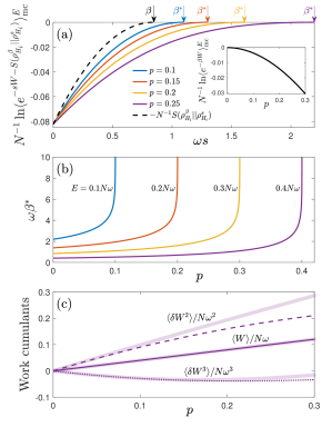
Figure 1: (a) Breakdown of the Jarzynski equality for a microcanonical ensemble of cyclically driven ($H_{f}=H_{i}$) two-level spins with $E=0.3N\omega$ and four transition rates $p$ (colored lines). Black arrow marks $\beta$ and colored arrows mark $\beta^{*}$ for each $p$. For a cyclic process Eq. (1) gives $\ln\langle e^{-\beta W}\rangle_{\mathrm{c}}^{\beta}=0$ whereas $\ln\langle e^{-\beta W}\rangle_{\mathrm{mc}}^{E}\neq 0$ for $p>0$ (note $S(\rho_{H_{i}}^{\beta}||\rho_{H_{i}}^{\beta})=0$). Instead $\ln\langle e^{-\beta^{*}W-S(\rho_{H_{i}}^{\beta}||\rho_{H_{i}}^{\beta^{*}})}\rangle_{\mathrm{mc}}^{E}=0$ in agreement with Eq. (13). The black-dashed line is $-N^{-1}S(\rho_{H_{i}}^{\beta}||\rho_{H_{i}}^{s})$. Inset: $\ln\langle e^{-\beta W}\rangle_{\mathrm{mc}}^{E}$ for $E=0.3N\omega$, which deviates from zero for increasing $p$, see Eq. (24). (b) The inverse temperature $\beta^{*}$ for four values of $E$. We have $\beta^{*}>\beta$ for $p>0$ and $\beta^{*}\rightarrow\infty$ for $p\rightarrow E/N\omega$. (c) First three microcanonical work cumulants $\langle W\rangle_{\mathrm{mc}}^{E}$ (dark-solid line), $\langle\delta W^{2}\rangle_{\mathrm{mc}}^{E}$ (dashed line) and $\langle\delta W^{3}\rangle_{\mathrm{mc}}^{E}$ (dotted line) for $E=0.3N\omega$. Corresponding canonical cumulants are shown by faint, thick, solid lines. The $n$th work cumulant has been scaled by $N\omega^{n}$.

Discussion.

We have shown that ensemble equivalence does not hold for the Jarzynski equality. We derive a modified relation that connects microcanonical work fluctuations to entropy production in an analogous way to the Jarzynski equality but with reference to a protocol-dependent inverse temperature $\beta^{*}$. This modified Jarzynski equality is a special case of a more general equation for the microcanonical moment-generating function for any extensive variable. We demonstrate the microcanonical Jarzynski equality in a system of non-interacting two-level spins. Interactions will increase the possible transitions between energy levels, in which case we expect deviation from MCE to be larger. Our results provide a useful starting point to consider fluctuation theorems from the perspective of the eigenstate thermalization hypothesis [70, 71, 72], as investigated numerically in [50]. Our results will be useful in systems where isolation is desirable, for example in quantum information systems [73], quantum simulators [74, 75] and ultracold-atom experiments. Connections with the microcanonical Crook’s relation [76, 45, 77, 78] is also an interesting area to explore.

References

- Gibbs [1902] J. W. Gibbs, Elementary Principles in Statistical Mechanics Developed with Especial Reference to the Rational Foundations of Thermodynamics (Charles Scribner’s Sons, New York, 1902).
- Touchette [2015] H. Touchette, Equivalence and nonequivalence of ensembles: Thermodynamic, macrostate, and measure levels, J. Stat. Phys. 159, 987 (2015).
- Lax [1955] M. Lax, Relation between canonical and microcanonical ensembles, Phys. Rev. 97, 1419 (1955).
- Lebowitz et al. [1967] J. L. Lebowitz, J. K. Percus, and L. Verlet, Ensemble dependence of fluctuations with application to machine computations, Phys. Rev. 153, 250 (1967).
- Lanford [1973] O. E. Lanford, Entropy and equilibrium states in classical statistical mechanics, in Statistical Mechanics and Mathematical Problems, edited by A. Lenard (Springer, Berlin, Heidelberg, 1973) pp. 1–113.
- Stroock and Zeitouni [1991] D. W. Stroock and O. Zeitouni, Microcanonical distributions, Gibbs states, and the equivalence of ensembles, in Random Walks, Brownian Motion, and Interacting Particle Systems: A Festschrift in Honor of Frank Spitzer, edited by R. Durrett and H. Kesten (Birkhäuser, Boston, MA, 1991) pp. 399–424.
- Cancrini and Olla [2017] N. Cancrini and S. Olla, Ensemble dependence of fluctuations: canonical microcanonical equivalence of ensembles, J. Stat. Phys. 168, 707 (2017).
- Sevick et al. [2008] E. Sevick, R. Prabhakar, S. R. Williams, and D. J. Searles, Fluctuation theorems, Annu. Rev. Phys. Chem. 59, 603 (2008).
- Campisi et al. [2011a] M. Campisi, P. Hänggi, and P. Talkner, Colloquium: Quantum fluctuation relations: Foundations and applications, Rev. Mod. Phys. 83, 771 (2011a).
- Jarzynski [1997a] C. Jarzynski, Nonequilibrium equality for free energy differences, Phys. Rev. Lett. 78, 2690 (1997a).
- Jarzynski [1997b] C. Jarzynski, Equilibrium free-energy differences from nonequilibrium measurements: A master-equation approach, Phys. Rev. E 56, 5018 (1997b).
- Schmiedl and Seifert [2007] T. Schmiedl and U. Seifert, Stochastic thermodynamics of chemical reaction networks, J. Chem. Phys. 126, 044101 (2007).
- Rao and Esposito [2018] R. Rao and M. Esposito, Conservation laws and work fluctuation relations in chemical reaction networks, J. Chem. Phys. 149, 245101 (2018).
- Qian [2005] H. Qian, Cycle kinetics, steady state thermodynamics and motors — a paradigm for living matter physics, J. Phys.: Condens. Matter 17, S3783 (2005).
- Ritort [2008] F. Ritort, Nonequilibrium fluctuations in small systems: From physics to biology, in Advances in Chemical Physics, Vol. 137, edited by S. A. Rice (John Wiley & Sons, Hoboken, New Jersey, 2008) pp. 31–123.
- Harris et al. [2007] N. C. Harris, Y. Song, and C.-H. Kiang, Experimental free energy surface reconstruction from single-molecule force spectroscopy using Jarzynski’s equality, Phys. Rev. Lett. 99, 068101 (2007).
- Gupta et al. [2011] A. N. Gupta, A. Vincent, K. Neupane, H. Yu, F. Wang, and M. T. Woodside, Experimental validation of free-energy-landscape reconstruction from non-equilibrium single-molecule force spectroscopy measurements, Nature Phys. 7, 631 (2011).
- Berkovich et al. [2013] R. Berkovich, J. Klafter, and M. Urbakh, Reconstruction of energy surfaces from friction force microscopy measurements with the Jarzynski equality, in Scanning Probe Microscopy in Nanoscience and Nanotechnology 3, edited by B. Bhushan (Springer, Berlin, Heidelberg, 2013) pp. 317–334.
- Liphardt et al. [2002] J. Liphardt, S. Dumont, S. B. Smith, I. Tinoco, and C. Bustamante, Equilibrium information from nonequilibrium measurements in an experimental test of Jarzynski’s equality, Science 296, 1832 (2002).
- Collin et al. [2005] D. Collin, F. Ritort, C. Jarzynski, S. B. Smith, I. J. Tinoco, and C. Bustamante, Verification of the Crooks fluctuation theorem and recovery of RNA folding free energies, Nature 437, 231 (2005).
- Douarche et al. [2005] F. Douarche, S. Ciliberto, A. Petrosyan, and I. Rabbiosi, An experimental test of the Jarzynski equality in a mechanical experiment, EPL 70, 593 (2005).
- Hoang et al. [2018] T. M. Hoang, R. Pan, J. Ahn, J. Bang, H. T. Quan, and T. Li, Experimental test of the differential fluctuation theorem and a generalized Jarzynski equality for arbitrary initial states, Phys. Rev. Lett. 120, 080602 (2018).
- Toyabe et al. [2010] S. Toyabe, T. Sagawa, M. Ueda, E. Muneyuki, and M. Sano, Experimental demonstration of information-to-energy conversion and validation of the generalized Jarzynski equality, Nature Phys. 6, 988 (2010).
- Saira et al. [2012] O.-P. Saira, Y. Yoon, T. Tanttu, M. Möttönen, D. V. Averin, and J. P. Pekola, Test of the Jarzynski and Crooks fluctuation relations in an electronic system, Phys. Rev. Lett. 109, 180601 (2012).
- Huber et al. [2008] G. Huber, F. Schmidt-Kaler, S. Deffner, and E. Lutz, Employing trapped cold ions to verify the quantum Jarzynski equality, Phys. Rev. Lett. 101, 070403 (2008).
- An et al. [2015] S. An, J.-N. Zhang, M. Um, D. Lv, Y. Lu, J. Zhang, Z.-Q. Yin, H. T. Quan, and K. Kim, Experimental test of the quantum Jarzynski equality with a trapped-ion system, Nature Phys. 11, 193 (2015).
- Xiong et al. [2018] T. P. Xiong, L. L. Yan, F. Zhou, K. Rehan, D. F. Liang, L. Chen, W. L. Yang, Z. H. Ma, M. Feng, and V. Vedral, Experimental verification of a Jarzynski-related information-theoretic equality by a single trapped ion, Phys. Rev. Lett. 120, 010601 (2018).
- Hahn et al. [2023] D. Hahn, M. Dupont, M. Schmitt, D. J. Luitz, and M. Bukov, Quantum many-body Jarzynski equality and dissipative noise on a digital quantum computer, Phys. Rev. X 13, 041023 (2023).
- Cerisola et al. [2017] F. Cerisola, Y. Margalit, S. Machluf, A. J. Roncaglia, J. P. Paz, and R. Folman, Using a quantum work meter to test non-equilibrium fluctuation theorems, Nat. Commun. 8, 1241 (2017).
- Liu et al. [2023] W. Liu, Z. Niu, W. Cheng, X. Li, C.-K. Duan, Z. Yin, X. Rong, and J. Du, Experimental test of the Jarzynski equality in a single spin-1 system using high-fidelity single-shot readouts, Phys. Rev. Lett. 131, 220401 (2023).
- Tasaki [2000] H. Tasaki, Jarzynski relations for quantum systems and some applications, arXiv:cond-mat/0009244 (2000).
- Yukawa [2000] S. Yukawa, A quantum analogue of the Jarzynski equality, J. Phys. Soc. Jpn. 69, 2367 (2000).
- Kurchan [2000] J. Kurchan, A quantum fluctuation theorem, arXiv:cond-mat/0007360 (2000).
- Mukamel [2003] S. Mukamel, Quantum extension of the Jarzynski relation: Analogy with stochastic dephasing, Phys. Rev. Lett. 90, 170604 (2003).
- Chernyak and Mukamel [2004] V. Chernyak and S. Mukamel, Effect of quantum collapse on the distribution of work in driven single molecules, Phys. Rev. Lett. 93, 048302 (2004).
- De Roeck and Maes [2004] W. De Roeck and C. Maes, Quantum version of free-energy–irreversible-work relations, Phys. Rev. E 69, 026115 (2004).
- Talkner et al. [2007] P. Talkner, E. Lutz, and P. Hänggi, Fluctuation theorems: Work is not an observable, Phys. Rev. E 75, 050102 (2007).
- Campisi et al. [2010] M. Campisi, P. Talkner, and P. Hänggi, Fluctuation theorems for continuously monitored quantum fluxes, Phys. Rev. Lett. 105, 140601 (2010).
- Campisi et al. [2011b] M. Campisi, P. Talkner, and P. Hänggi, Influence of measurements on the statistics of work performed on a quantum system, Phys. Rev. E 83, 041114 (2011b).
- Hänggi and Talkner [2015] P. Hänggi and P. Talkner, The other QFT, Nature Phys. 11, 108 (2015).
- Åberg [2018] J. Åberg, Fully quantum fluctuation theorems, Phys. Rev. X 8, 011019 (2018).
- Bartolotta and Deffner [2018] A. Bartolotta and S. Deffner, Jarzynski equality for driven quantum field theories, Phys. Rev. X 8, 011033 (2018).
- Park and Schulten [2004] S. Park and K. Schulten, Calculating potentials of mean force from steered molecular dynamics simulations, J. Chem. Phys. 120, 5946 (2004).
- Jarzynski [2000] C. Jarzynski, Hamiltonian derivation of a detailed fluctuation theorem, J. Stat. Phys 98, 77 (2000).
- Cleuren et al. [2006] B. Cleuren, C. Van den Broeck, and R. Kawai, Fluctuation and dissipation of work in a Joule experiment, Phys. Rev. Lett. 96, 050601 (2006).
- Subaş ı and Jarzynski [2013] Y. Subaş ı and C. Jarzynski, Microcanonical work and fluctuation relations for an open system: An exactly solvable model, Phys. Rev. E 88, 042136 (2013).
- Schmidtke et al. [2018] D. Schmidtke, L. Knipschild, M. Campisi, R. Steinigeweg, and J. Gemmer, Stiffness of probability distributions of work and Jarzynski relation for non-Gibbsian initial states, Phys. Rev. E 98, 012123 (2018).
- Knipschild et al. [2021] L. Knipschild, A. Engel, and J. Gemmer, Stiffness of probability distributions of work and Jarzynski relation for initial microcanonical and energy eigenstates, Phys. Rev. E 103, 062139 (2021).
- Jeon et al. [2015] E. Jeon, Y. W. Kim, and J. Yi, Initial ensemble dependence of Jarzynski equality in the thermodynamic limit, J. Phys. A: Math. Theor. 48, 305002 (2015).
- Jin et al. [2016] F. Jin, R. Steinigeweg, H. De Raedt, K. Michielsen, M. Campisi, and J. Gemmer, Eigenstate thermalization hypothesis and quantum Jarzynski relation for pure initial states, Phys. Rev. E 94, 012125 (2016).
- Yi et al. [2011] J. Yi, P. Talkner, and M. Campisi, Nonequilibrium work statistics of an Aharonov-Bohm flux, Phys. Rev. E 84, 011138 (2011).
- Atas et al. [2020] Y. Y. Atas, A. Safavi-Naini, and K. V. Kheruntsyan, Nonequilibrium quantum thermodynamics of determinantal many-body systems: Application to the Tonks-Girardeau and ideal Fermi gases, Phys. Rev. A 102, 043312 (2020).
- Gong and Quan [2015] Z. Gong and H. T. Quan, Jarzynski equality, Crooks fluctuation theorem, and the fluctuation theorems of heat for arbitrary initial states, Phys. Rev. E 92, 012131 (2015).
- Wong [1989] R. Wong, Asymptotic approximations of integrals (Academic Press, Boston, San Diego, New York, 1989).
- Ahlfors [1979] L. V. Ahlfors, Complex Analysis, 3rd ed. (McGraw-Hill, New York, 1979).
-
Note [1]
In detail,
The integral can be evaluated using Laplace’s method (the real-space equivalent of the saddle-point approximation), which gives
This combined with Eq. (7\@@italiccorr) identifies the saddle-point energy as the energy that gives . Noting that gives Eq. (1\@@italiccorr). - Cover and Thomas [2006] T. M. Cover and J. A. Thomas, Elements of information theory, 2nd ed. (John Wiley & Sons, Hoboken, New Jersey, 2006).
- Vedral [2002] V. Vedral, The role of relative entropy in quantum information theory, Rev. Mod. Phys. 74, 197 (2002).
- Pusz and Woronowicz [1978] W. Pusz and S. L. Woronowicz, Passive states and KMS states for general quantum systems, Commun. Math. Phys. 58, 273 (1978).
- Deffner and Lutz [2010] S. Deffner and E. Lutz, Generalized Clausius inequality for nonequilibrium quantum processes, Phys. Rev. Lett. 105, 170402 (2010).
- Dorner et al. [2012] R. Dorner, J. Goold, C. Cormick, M. Paternostro, and V. Vedral, Emergent thermodynamics in a quenched quantum many-body system, Phys. Rev. Lett. 109, 160601 (2012).
- Allen and Eberly [1987] L. Allen and J. H. Eberly, Optical resonance and two-level atoms (Dover Publications, New York, 1987).
- Ramsey [1956] N. F. Ramsey, Thermodynamics and statistical mechanics at negative absolute temperatures, Phys. Rev. 103, 20 (1956).
-
Note [2]
We write and combine the factor with to
obtain
where we have used the binomial identity
The factor can be combined with the factor to obtain Eq. (22\@@italiccorr) after using the binomial identity a second time. - Allahverdyan and Nieuwenhuizen [2005] A. E. Allahverdyan and T. M. Nieuwenhuizen, Minimal work principle: Proof and counterexamples, Phys. Rev. E 71, 046107 (2005).
- Polkovnikov [2008] A. Polkovnikov, Microscopic expression for heat in the adiabatic basis, Phys. Rev. Lett. 101, 220402 (2008).
- Polkovnikov [2011] A. Polkovnikov, Microscopic diagonal entropy and its connection to basic thermodynamic relations, Ann. Phys. 326, 486 (2011).
- Santos et al. [2011] L. F. Santos, A. Polkovnikov, and M. Rigol, Entropy of isolated quantum systems after a quench, Phys. Rev. Lett. 107, 040601 (2011).
-
Note [3]
Explicitly, we obtain
Note the scaling does not hold in general for . - Deutsch [1991] J. M. Deutsch, Quantum statistical mechanics in a closed system, Phys. Rev. A 43, 2046 (1991).
- Srednicki [1994] M. Srednicki, Chaos and quantum thermalization, Phys. Rev. E 50, 888 (1994).
- Rigol et al. [2008] M. Rigol, V. Dunjko, and M. Olshanii, Thermalization and its mechanism for generic isolated quantum systems, Nature 452, 854 (2008).
- Auffèves [2022] A. Auffèves, Quantum technologies need a quantum energy initiative, PRX Quantum 3, 020101 (2022).
- Georgescu et al. [2014] I. M. Georgescu, S. Ashhab, and F. Nori, Quantum simulation, Reviews of Modern Physics 86, 153 (2014).
- Altman et al. [2021] E. Altman, K. R. Brown, G. Carleo, L. D. Carr, E. Demler, C. Chin, B. DeMarco, S. E. Economou, M. A. Eriksson, K.-M. C. Fu, M. Greiner, K. R. Hazzard, R. G. Hulet, A. J. Kollár, B. L. Lev, M. D. Lukin, R. Ma, X. Mi, S. Misra, C. Monroe, K. Murch, Z. Nazario, K.-K. Ni, A. C. Potter, P. Roushan, M. Saffman, M. Schleier-Smith, I. Siddiqi, R. Simmonds, M. Singh, I. Spielman, K. Temme, D. S. Weiss, J. Vučković, V. Vuletić, J. Ye, and M. Zwierlein, Quantum simulators: Architectures and opportunities, PRX Quantum 2, 017003 (2021).
- Crooks [1999] G. E. Crooks, Entropy production fluctuation theorem and the nonequilibrium work relation for free energy differences, Phys. Rev. E 60, 2721 (1999).
- Talkner et al. [2008] P. Talkner, P. Hänggi, and M. Morillo, Microcanonical quantum fluctuation theorems, Phys. Rev. E 77, 051131 (2008).
- Talkner et al. [2013] P. Talkner, M. Morillo, J. Yi, and P. Hänggi, Statistics of work and fluctuation theorems for microcanonical initial states, New J. Phys. 15, 095001 (2013).