Consensus in Models for Opinion Dynamics with Generalized-Bias

Abstract

Interest is growing in social learning models where users share opinions and adjust their beliefs in response to others. This paper introduces generalized-bias opinion models, an extension of the DeGroot model, that captures a broader range of cognitive biases. These models can capture, among others, dynamic (changing) influences as well as in-group favoritism and out-group hostility, a bias where agents may react differently to opinions from members of their own group compared to those from outside. The reactions are formalized as arbitrary functions that depend, not only on opinion difference, but also on the particular opinions of the individuals interacting. Under certain reasonable conditions, all agents –despite their biases– will converge to a consensus if the influence graph is strongly connected, as in the original DeGroot model. The proposed approach combines different biases, providing deeper insights into the mechanics of opinion dynamics and influence within social networks.

1 Introduction

Social networks have played a significant role in shaping users’ opinions, often influencing democratic processes and contributing to social polarization. Broadly, the dynamics of opinion formation in social networks involve users expressing their views, encountering the opinions of others, and potentially updating their own beliefs based on these interactions. There is a growing interest in developing models of social learning  [21] capturing these dynamics to gain insights on how opinions form and spread within social networks.

The DeGroot model [9] is perhaps the most prominent framework for social learning and opinion formation dynamics. In this model, a community is represented as a weighted directed graph, known as the influence graph, with edges indicating how much individuals (agents) influence one another. Each agent has an opinion represented as a value in the interval $[0,1]$, indicating the strength of the agreement with an underlying proposition (e.g., “AI poses a threat to humanity”). Agents revise their opinions by “averaging” them with those of their contacts, weighted by their influence. Studies support the validity of opinion formation, in many cases, by averaging as demonstrated in controlled sociological experiments [6].

A key theoretical result about the model states that the agents will converge to consensus if the influence graph is strongly connected and the agents have non-zero self-influence (puppet freedom is assumed) [12]. The significance of this result lies in the fact that consensus is a central problem in social learning. Indeed, the inability to reach consensus is a sign of a polarized community. The DeGroot model is valued for its tractability, derived from its connection with matrix powers and Markov chains; it remains a significant focus of study for understanding of opinion evolution [12].

The DeGroot model, however, assumes two constraints that could be overly demanding in the context of social networks. It assumes homogeneity and linearity of opinion update dynamics. In social scenarios, two agents may update their opinions differently depending on their individual cognitive biases on disagreement (i.e., on how they interpret and react towards the level of disagreements with others). This results in more involved updates that may rely on non-linear, even non-monotonic, functions. For example, an individual under confirmation (cognitive) bias [4] may ignore the opinion of those whose level of disagreement is over a certain threshold. A recent work [2] introduces an extension of the DeGroot model that allows for some form of heterogeneous and non-linear opinion updates. The model takes disagreement between agents as one of its key parameters.

Nevertheless, representing cognitive biases solely as functions of disagreement [2] overlooks key behaviors where reactions to the same opinion can vary greatly depending on whether the opposing view comes from someone within their own political group. This can be attributed to in-group favoritism (or out-group hostility), which are aspects of inter-group bias and social identity theory [19]. In order to capture these nuances, models of cognitive biases need to incorporate factors beyond mere, isolated, disagreement.

This paper introduces generalized-bias opinion models, a framework that generalizes the aforementioned models: it can capture a broader range of cognitive biases formalized as arbitrary functions that depend, not only on opinion disagreement, but also on the opinions of the individuals involved. It is demonstrated that the proposed framework can effectively represent standard cognitive biases of significant relevance in social networks. These include, among others, confirmation and identity-based inter-group biases [19], where users are more inclined to favor opinions from people within their own ideological group. It also allows for modelling dynamic (changing) influences. The approach allows for the combination and integration of these biases, enabling a more comprehensive and formal understanding of opinion dynamics and influence in social networks.

Furthermore, the key result of the DeGroot model is extended by demonstrating that, under certain reasonable conditions, all agents—despite being subject to the aforementioned cognitive biases—will converge to a consensus if the influence graph is strongly connected. This highlights the robustness of the proposed framework in achieving consensus even when accounting for complex, arbitrary bias-driven dynamics under some reasonable conditions. Additionally, it is also shown that the proposed framework allows for more expressive models to those introduced in [1, 2, 9]. These results contribute to a richer representation of human cognition and interaction in social networks. Indeed, the framework is illustrated with a case-study modelling inter-group bias.

2 Preliminaries

This paper uses notation and background from linear algebra [15]. This section summarizes the main aspects of the notation and the background. Further details on special types of matrices and dynamical systems [5] can be found in Appendix A.

The term $N$ is a positive integer and is used to identify the number of agents in a network. The expressions $\mathbb{R}^{N}$ and $\mathbb{R}^{N\times N}$ denote the collections, respectively, of real-valued vectors of length $N$ and real-valued squared matrices of side $N$. Boldface lowercase letters identify vectors in $\mathbb{R}^{N}$ and boldface uppercase letters identify matrices in $\mathbb{R}^{N\times N}$. The expression $\mathbf{I}$ denotes the identity matrix in $\mathbb{R}^{N\times N}$ and $\mathrm{det}(\_)$ the determinant (partial) function on matrices. Recall that if the inverse $\mathbf{A}^{-1}$ of $\mathbf{A}$ exists, it satisfies $\mathbf{A}\mathbf{A}^{-1}=\mathbf{A}^{-1}\mathbf{A}=\mathbf{I}$. The L1 norm of a vector $\mathbf{x}$ is denoted $\left\lVert\mathbf{x}\right\rVert_{1}$. When the values of a vector $\mathbf{x}$ need to be made explicit, it can be denoted as $\mathbf{x}=\left[x_{i}\right]_{i\in I}$ or $\left[x_{i}\right]$ when the index set $I$ can be inferred from the context. Similarly, when the values of a matrix $\mathbf{A}$ need to be made explicit, it can be denoted as $\mathbf{A}=\left[a_{ij}\right]_{(i,j)\in I\times J}$ or $\left[a_{ij}\right]$ when the index sets $I$ and $J$ can be inferred from the context. It is said that $\mathbf{A}$ is non-negative, denoted $\mathbf{A}\geq 0$, iff $a_{ij}\geq 0$ for $1\leq i,j\leq N$. Likewise, $\mathbf{A}$ is positive, denoted $\mathbf{A}>0$, iff $a_{ij}>0$ for $1\leq i,j\leq N$. A matrix $\mathbf{A}$ is primitive iff $\mathbf{A}^{m}>0$ for some $m\in\mathbb{N}$ [15]. A (square) matrix $\mathbf{P}$ is called a permutation matrix when it has exactly one entry of 1 in each row and each column, and 0s elsewhere. A matrix $\mathbf{A}$ is reducible if there is a permutation matrix $\mathbf{P}$ such that $\mathbf{P}^{T}\mathbf{A}\mathbf{P}=\begin{bmatrix}\mathbf{B}&\mathbf{C}\\ \mathbf{0}&\mathbf{D}\end{bmatrix}$ where $\mathbf{B}$ and $\mathbf{D}$ are square matrices (possibly of different sizes), $\mathbf{C}$ is a matrix of appropriate size, and $\mathbf{0}$ is the zero matrix of appropriate size. If no such permutation matrix $\mathbf{P}$ exists, then $\mathbf{A}$ is called irreducible.

A non-zero vector $\mathbf{x}$ is an eigenvector of a matrix $\mathbf{A}$ with eigenvalue $\lambda\in\mathbb{C}$ iff $\mathbf{A}\mathbf{x}=\lambda\mathbf{x}$ (i.e., applying $\mathbf{A}$ to the eigenvector $\mathbf{x}$ only scales the eigenvector by the scalar value $\lambda$). The spectrum of $\mathbf{A}$ is the set $\sigma(\mathbf{A})$ of all eigenvalues $\lambda$ satisfying the equation $\mathrm{det}(\mathbf{A}-\lambda\mathbf{I})=0$. The geometric multiplicity of $\lambda\in\sigma(\mathbf{A})$, denoted $m_{g}(\lambda)$, is the number of eigenvectors associated to $\lambda$ in the (spectral) decomposition of $\mathbf{A}$. The algebraic multiplicity of $\lambda\in\sigma(\mathbf{A})$, denoted $m_{a}(\lambda)$, is the number of times $\lambda$ appears as a root of the characteristic polynomial of $\mathbf{A}$. It is known that $m_{g}(\lambda)\leq m_{a}(\lambda)$ for any $\lambda\in\sigma(\mathbf{A})$. The spectral radius of $\mathbf{A}$ is the real value $\rho(\mathbf{A})$ defined by $\rho(\mathbf{A})=\max_{\lambda\in\sigma(A)}\left|\lambda\right|$ identifying the greatest magnitude among all eigenvalues of $\mathbf{A}$. If $\lambda\in\sigma(\mathbf{A})$ and it is the only eigenvalue that satisfies $|\lambda|=\rho(\mathbf{A})$, then $\lambda$ is called the dominant eigenvalue of $\mathbf{A}$.

The Perron-Frobenius Theorem [15] is a fundamental result about non-negative matrices. For irreducible $\mathbf{A}\in\mathbb{R}^{N\times N}\geq 0$, there exists a real and positive eigenvalue $\lambda_{1}=\rho(\mathbf{A})$, called the Perron-Frobenius eigenvalue, there exists a corresponding eigenvector $\mathbf{v}$ to $\lambda_{1}$, called the Perron-Frobenius eigenvector, such that $\mathbf{v}$ has positive components (it can always be picked to have Euclidean norm equal to 1), and the eigenvalue $\lambda_{1}$ is simple in the sense that $m_{a}(\lambda_{1})=1$.

3 Generalized-bias Opinion Models

This section presents a generalization of the DeGroot model to capture biases on opinion differences. It can account, among others, for dynamic influence/weights and inter-group biases [14] where agents favor one’s own group over other groups.

In social learning models, a community, society, or network is typically represented as a directed weighted graph. The edges between individuals (agents) specify the direction and strength of the influence that one carries over the other.

Definition 3.1.

An ($N$-agent) influence graph is a directed weighted graph $G=(A,E,I)$ with vertices $A=\left\{1,\ldots N\right\}$, edges $E\subseteq A\times A$, and weight function $I=A\times A\to\left[0,1\right]$ satisfying $I(i,j)=0$ iff $(i,j)\notin E$.

The vertices $A$ represent the $N$ agents of a given community or network. Whenever $(i,j)\in E$, it means that agent $i$ influences agent $j$. The value $I(i,j)$, for simplicity written $I_{i,j}$, denotes the strength of the influence: $0$ means no influence and a higher value means stronger influence. The expression $A_{i}$ is used to denote the set of (inbound-)neighbors of agent $i$, i.e., the set of agents $j$ with $I_{j,i}>0$. Recall that a graph is strongly connected if there is at least one path between any two vertices. In a strongly connected influence graph, all the agents influence –directly or indirectly– one another.

The evolution of agents’ opinions, about some underlying statement or proposition, is modeled similar to the DeGroot-like models in [9, 1, 2].

An opinion state (or belief state) of the $N$ agents is represented as a vector in $\left[0,1\right]^{N}$. For any opinion state $\mathbf{x}=\left[x_{1},\ldots,x_{N}\right]$ and $1\leq i\leq N$, the expression $\mathbf{x}_{i}=x_{i}$ denotes the opinion of agent $i$. If $\mathbf{x}_{i}=0$, then $i$ completely disagrees with the proposition; if $\mathbf{x}_{i}=1$, then $i$ completely agrees with it. The higher the value of $\mathbf{x}_{i}$, the stronger the agreement.

Definition 3.2.

An opinion model is a tuple $M=\left(G,\mathbf{x}^{0},\mu_{G}\right)$, where G is an N-agent influence graph, $\mathbf{x}^{0}$ is the initial state of opinion, and $\mu_{G}:\left[0,1\right]^{N}\to\left[0,1\right]^{N}$ is a state-transition function, called update function. For every $t\in\mathbb{N}$, $\mathbf{x}^{t+1}=\mu_{G}(\mathbf{x}^{t})$ is the state of opinion at time $t+1$ in $M$.

An update function can be used to express any deterministic and discrete transition from one opinion state to the next, possibly taking into account the influence graph. Intuitively, these update functions specify the reaction of an agent to the opinion disagreements with each one of its influencers.

Consensus is a central property in social learning (e.g., the inability to reach consensus is a sign of a polarized society).

Definition 3.3.

Let $\left(G,\mathbf{x}^{0},\mu_{G}\right)$ be an opinion model with $G=\left(A,E,I\right)$. A subset of agents $B\subseteq A$ is said to converge to an opinion value $v$ iff for every $i\in B$, $\lim_{t\to\infty}\mathbf{x}^{t}_{i}=v$. The subset $B$ is said to converge to consensus iff $B$ converges to some opinion value $v$.

3.1 DeGroot Update

The normalized influence $\overline{I_{j,i}}=\frac{I_{j,i}}{\sum_{k\in A_{i}}I_{k,i}}$ is used to model the opinion update of agent $i$ as a function of its neighbors’ opinions [2]. Then, the standard DeGroot model [9] is obtained by the update function $\mu_{G}(\mathbf{x})_{i}=\sum_{j\in A_{i}}\overline{I_{j,i}}\mathbf{x}_{j}$ which can be equivalently formulated as in Equation 1:

$$\mu_{G}(\mathbf{x})_{i} =\mathbf{x}_{i}+\sum_{j\in A_{i}}\overline{I_{j,i}}(\mathbf{x}_{j}-\mathbf{x}_{i}).$$ (1)

If $j$ influences $i$, then $i$’s opinion would tend to move closer to $j$’s. The disagreement term $(\mathbf{x}_{j}-\mathbf{x}_{i})\in[-1,1]$ in Equation 1 realizes this intuition. If $(\mathbf{x}_{j}-\mathbf{x}_{i})$ is a negative term in the sum, the disagreement can be thought of as contributing with a magnitude of $|\mathbf{x}_{j}-\mathbf{x}_{i}|$ (multiplied by $\overline{I_{j,i}}$) to decreasing $i$’s belief in the underlying proposition. Similarly, if $(\mathbf{x}_{j}-\mathbf{x}_{i})$ is positive, the disagreement contributes with the same magnitude but to increasing $i$’s belief.

It is known that in standard DeGroot, two conditions on the influence graph are enough for the agents converge to consensus. First, the all the agents are required to influence, directly or indirectly, each other. Second, each agent has to have some self-influence.

Theorem 3.4 ([9]).

Let $\left(G,\mathbf{x}^{0},\mu_{G}\right)$ be an opinion model with $G=\left(A,E,I\right)$ and $\mu_{G}$ defined by Eq. 1. If $G$ is (1) strongly connected and (2) for each $i\in A$, $\overline{I_{j,i}}<1$ for some $j\in A_{i}$, then $A$ converges to consensus.

3.2 Updates with Bias Factors

A broad class of update functions, generalizing the original one in DeGroot, is introduced in this section. More precisely, updates for an agent $i$ can weight disagreements with each one of its neighbors $j$ using functions $\alpha_{ij}$ from opinion states to $[0,1]$ referred to as (generalized) bias factors. The same opinion difference can then be weighted differently by bias factors, depending of opinions of agents $i$ and $j$. Thus, intuitively $\alpha_{ij}$ may also be seen as changing the influence of $j$ over $i$ depending on their opinions.

As an example, assume that $0.5$ represents a neutral opinion about an underlying proposition. If $\mathbf{x}_{i}=0.4$ and $\mathbf{x}_{j}=0.1$, the agents can be viewed as somewhat disagreeing and strongly disagreeing, respectively, with the underlying proposition. If $\mathbf{x}_{i}=0.7$ and $\mathbf{x}_{j}=0.4$, agent $i$ seems to agree somewhat with the proposition, while $j$ does not. Alas, in both cases $(\mathbf{x}_{j}-\mathbf{x}_{i})=0.3$. It could be desirable to have $\alpha_{i,j}(\mathbf{x})$ assigning a higher weight in the first situation because these opinions come from a group that disagrees with the proposition. (This cannot be achieved with the influence graph alone since the opinion of agents may change while their influence in an opinion model does not.) As a matter of fact, this is an instance of in-group bias.

Definition 3.5.

Let $\left(G,\mathbf{x}^{0},\mu_{G}\right)$ be an opinion model with $G=\left(A,E,I\right)$. The function $\mu_{G}:\left[0,1\right]\to\left[0,1\right]$ is an generalized bias update iff, for each $i\in A$, it is defined by:

$$\mu_{G}(\mathbf{x})_{i} =\mathbf{x}_{i}+\sum_{j\in A_{i}}\overline{I_{j,i}}\alpha_{i,j}(\mathbf{x})(\mathbf{x}_{j}-\mathbf{x}_{i}),$$ (2)

with each bias factor $\alpha_{i,j}:\left[0,1\right]^{N}\to\left[0,1\right]$ satisfying:

1. $\alpha_{i,j}$ is a continuous function,

2. if $\mathbf{x}_{i}\neq\mathbf{x}_{j}$, then $\alpha_{i,j}(\mathbf{x})>0$, and

3. for each $i\in A$, there exists $j\in A_{i}$, such that $\alpha_{i,j}(\mathbf{x})<1$.

The first condition on the bias factor $\alpha_{i,j}$ guarantees that small changes in the state of opinion lead to small changes in the factor result. Without the second condition, the bias factor would cancel the influence of the contact $j$, which may break the strong connectivity of the graph. The third and last condition reproduces the second condition in the Theorem 3.4 in the original DeGroot model.

Note that the update function in Equation 2 can be expressed equivalently as:

$$\mu_{G}(\mathbf{x})_{i} =\left(1-\sum_{j\in A_{i}}\overline{I_{j,i}}\alpha_{i,j}(\mathbf{x})\right)\mathbf{x}_{i}+\sum_{j\in A_{i}}\overline{I_{j,i}}\alpha_{i,j}(\mathbf{x})\mathbf{x}_{j},$$ (3)

Furthemore, Equation 2 is a convex combination of $\left[0,1\right]$ elements and thus $\mu_{G}(\mathbf{x})_{i}\in\left[0,1\right]$ because $\left[0,1\right]$ is a convex set. Consequently, the generalized-bias update function can be expressed in vectorial form as:

$$\mu_{G}(\mathbf{x}) =\mathbf{A}(\mathbf{x})\mathbf{x},$$ (4)

where $\mathbf{A}:\left[0,1\right]^{N}\to\mathbb{R}^{N\times N}$ is a square matrix with entries

$$a_{i,j}(\mathbf{x})=\left\{\begin{array}[]{lcc}\vspace{0.5cm}1-\sum_{k\in A_{i}}\overline{I_{k,i}}\alpha_{i,k}(\mathbf{x})&\quad\mbox{, if}&i=j\\ \overline{I_{j,i}}\alpha_{i,j}(\mathbf{x})&\quad\mbox{, if}&i\neq j.\end{array}\right.$$ (7)

This section is concluded by introducing the notion of generalized bias opinion models.

Definition 3.6.

Let $M=\left(G,\mathbf{x}^{0},\mu_{G}\right)$ be an opinion model with $G=\left(A,E,I\right)$. Then, $M$ is an generalized-bias (opinion) model iff $\mu_{G}$ can be expressed as in Equation 4.

4 Consensus and Expressiveness

This section presents a consensus result for generalized-bias opinion models (Definition 3.6). It is the main theoretical result of the paper and extends the DeGroot’s consensus result (see Theorem 3.4). This section also shows how generalized-bias models capture the opinion specification and dynamics of other models, including state-of-the-art [1, 2, 9]. It highlights dynamics that generalized-bias models can handle, but the other models cannot.

Lemma 4.1.

Let $\left(G,\mathbf{x}^{0},\mu_{G}\right)$ be an generalized-bias model, with $G=\left(A,E,I\right)$ and $\mu_{G}(\mathbf{x})=\mathbf{A}(\mathbf{x})\mathbf{x}$. The matrix $\mathbf{A}(\mathbf{x})$ is (right-)stochastic for all $\mathbf{x}\in\left[0,1\right]^{N}$.

Recall that a matrix $\mathbf{A}=\left[a_{ij}\right]\in\mathbb{R}^{N\times N}$ is (right-)stochastic if it entries satisfy $a_{ij}\geq 0$ and $\sum^{N}_{j=1}a_{ij}=1$. This guarantees that consensual state of opinion vectors (i.e., vectors in which all agents have the same opinion) in generalized-bias models are fixed points of their update function. Intuitively, this means that once the agents are in consensus, they will remain in consensus.

Lemma 4.2.

Let $\left(G,\mathbf{x}^{0},\mu_{G}\right)$ be a generalized-bias model, with $G=\left(A,E,I\right)$ and $\mu_{G}(\mathbf{x})=\mathbf{A}(\mathbf{x})\mathbf{x}$. If $G$ is a strongly connected graph, then for every $t>0$, $\mathbf{A}(\mathbf{x}^{t})$ is primitive.

Genelarized-bias models have unique fixed points. The primitivity of $\mathbf{A}(\mathbf{x}_{t})$, for $t>0$, indicates that they are consensual vectors. This is a key observation for proving that generalized-bias models converge to consensus, as it ensures that for each state opinion vector $\mathbf{x}^{t}$, its update $\mathbf{x}^{t+1}$ is closer to consensus than $\mathbf{x}^{t}$.

Theorem 4.3 (Consensus for Generalized-Bias Models).

Let $\left(G,\mathbf{x}^{0},\mu_{G}\right)$ be a generalized-bias model, with $G=\left(A,E,I\right)$ and $\mu_{G}(\mathbf{x})=\mathbf{A}(\mathbf{x})\mathbf{x}$. If $G$ is a strongly connected graph, then $A$ converges to consensus.

The connectivity constraint on $G$ ensures that each pair of agents $(i,j)$ is connected, directly or indirectly. Hence, the opinion of $i$ is in a certain way influenced by the opinion of $j$ and viceversa. The non-zero condition of the the bias factors ensures that no matter the difference of opinions between two agents, if there is a connection between them, this influence, and hence their disagreement, will not be ignored but it would be dynamically weighted. Intuitively, the generalized-bias models guarantee that in an environment where all users can freely express their opinions and be heard, they will eventually come to an agreement even if there are certain cognitive biases that regulate the influences between them.

The proofs of the above lemmas and Theorem 4.3 can be found in Appendix B.

Expressiveness of Generalized-Bias Models.

The work in [2] introduces disagreement-bias (opinion) models. They are extensions of DeGroot’s of the form $\left(G,\mathbf{x}^{0},\mu_{G}\right)$ with

$$\mu_{G}(\mathbf{x})_{i} =\mathbf{x}_{i}+\sum_{j\in A_{i}}\overline{I_{j,i}}\beta_{i,j}(\mathbf{x}_{j}-\mathbf{x}_{i}),$$ (8)

where each $\beta_{i,j}:\left[-1,1\right]\to\left[-1,1\right]$ is a function referred to as disagreement bias. Intuitively, $\beta_{i,j}(\mathbf{x}_{j}-\mathbf{x}_{i})$ is a factor that depends only on the difference of opinion between $j$ and $i$.

It is shown that the agents in a disagreement-bias model converge to consensus if its influence graph is strongly connected and each $\beta_{i,j}$ function is continuous and in the region $\mbox{{R}}=\left\{(x,y)\in\left[-1,1\right]^{2}:xy>0\mbox{ and }\left|y\right|<\left|x\right|\right\}\cup\left\{(0,0)\right\}$. The models with all their bias functions in R can capture a wide range of biases, such as variations of confirmation bias as well as the dynamics of receptive and resistant agents (i.e., agents willing to change their opinion towards their contacts but with some skepticism) [4].

Theorem 4.4 ([2]).

Let $\left(G,\mathbf{x}^{0},\mu_{G}\right)$ with $G=\left(A,E,I\right)$ be a disagreement-bias model whose disagreement bias functions are continuous and in R. If $G$ is strongly connected, $A$ converges to consensus.

Theorem 4.4 is actually a consequence of Theorem 4.3 from this paper. It can be shown that the update functions of disagreement-bias models, whose continuous bias functions are in $\mathbf{R}$, can be expressed as update functions of generalized-bias models. It can also be shown that there are updates functions from generalized-bias models that cannot be expressed as the update functions of a disagreement-bias model. More precisely,

Theorem 4.5 (Expressiveness).

(1) Let $(G,\mathbf{x}^{0},\nu_{G})$ be a disagreement-bias model whose disagreement bias functions are continuous and in $\mathbf{R}$. Then, there exists a generalized-bias model $(G,\mathbf{x}^{0},\mu_{G})$, such that $\mu_{G}=\nu_{G}$. (2) There exists a generalized-bias model $(G,\mathbf{x}^{0},\mu_{G})$ such that every disagreement-bias model $(G,\mathbf{x}^{0},\nu_{G})$ satisfies $\mu_{G}\neq\nu_{G}$.

Proof.

Part (1). Given any disagreement-bias model $(G,\mathbf{x}^{0},\nu_{G})$ whose disagreement biases are continuous and in $\mathbf{R}$, define the generalized-bias model $(G,\mathbf{x}^{0},\mu_{G})$ where:

$$\alpha_{i,j}(\mathbf{x}) =\left\{\begin{array}[]{lcc}\vspace{0.5cm}\frac{\beta_{i,j}(\mathbf{x}_{j}-\mathbf{x}_{i})}{\mathbf{x}_{j}-\mathbf{x}_{i}}&\mbox{\quad, if}&\mathbf{x}_{j}\neq\mathbf{x}_{i},\\ 0&\mbox{\quad, if}&\mathbf{x}_{j}=\mathbf{x}_{i}.\end{array}\right.$$ (11)

Here, $\beta_{i,j}$ is the corresponding disagreement bias in $(G,\mathbf{x}^{0},\nu_{G})$. It can be verified that $0<\alpha_{i,j}(\mathbf{x})<1$. Also, $\alpha_{i,j}$ is continuous because $\beta_{i,j}$ is continuous. Thus, $\alpha_{i,j}$ satisfies the conditions for the bias factors in Definition 3.5; it can be verified that $\mu_{G}=\nu_{G}$.

For Part (2), consider the generalized-bias model $(G,\mathbf{x}^{0},\mu_{G})$, with $G=(A,E,I)$, $A=\left\{1,2\right\}$, $E=\left\{(1,2),(2,1)\right\}$, and $I_{12}=I_{21}=1.0$, and:

$$\mu_{G}(\mathbf{x})_{1} =\mathbf{x}_{1}+\alpha_{12}(\mathbf{x}_{1},\mathbf{x}_{2})(\mathbf{x}_{2}-\mathbf{x}_{1}), \mu_{G}(\mathbf{x})_{2} =\mathbf{x}_{2}+\alpha_{21}(\mathbf{x}_{1},\mathbf{x}_{2})(\mathbf{x}_{2}-\mathbf{x}_{1}).$$ (12)

Suppose that $\alpha_{12}(\mathbf{x}_{1},\mathbf{x}_{2})=\alpha_{21}(\mathbf{x}_{1},\mathbf{x}_{2})=\alpha(\mathbf{x}_{1},\mathbf{x}_{2})$, where

$$\alpha(\mathbf{x})=\alpha(\mathbf{x}_{1},\mathbf{x}_{2})=2\left(\mathbf{x}_{1}-\mathbf{x}^{2}_{1}+0.25\right)\left(1-0.9\left|\mathbf{x}_{1}-\mathbf{x}_{2}\right|\right).$$ (13)

Towards of contradiction, suppose that there exists a disagreement-bias model $(G,\mathbf{x}^{0},\nu_{G})$ such that $\nu_{G}=\mu_{G}$. Then, the update function $\nu_{G}$ must have the form

$$\nu_{G}(\mathbf{x})_{1} =\mathbf{x}_{1}+\beta_{12}(\mathbf{x}_{2}-\mathbf{x}_{1}) \nu_{G}(\mathbf{x})_{2} =\mathbf{x}_{2}+\beta_{21}(\mathbf{x}_{1}-\mathbf{x}_{2}),$$ (14)

with $\beta_{12}(\mathbf{x}_{1}-\mathbf{x}_{2})=\alpha_{12}(\mathbf{x}_{1},\mathbf{x}_{2})(\mathbf{x}_{2}-\mathbf{x}_{1})$ and $\beta_{21}(\mathbf{x}_{2}-\mathbf{x}_{1})=\alpha_{21}(\mathbf{x}_{1},\mathbf{x}_{2})(\mathbf{x}_{2}-\mathbf{x}_{1})$. However, for the opinion states $\mathbf{y}=\left[0,0.2\right]$ and $\mathbf{z}=\left[0.5,0.7\right]$, it follows that $-0.2\alpha_{12}(0,0.2)=\beta_{21}(-0.2)=-0.2\alpha_{12}(0.5,0.7)$. This is a contradiction because $\alpha_{12}(0,0.2)=0.41$ and $\alpha_{12}(0.5,0.7)=0.82$.∎

5 Intergroup Bias: A Case Study

Intergroup bias is a well-documented phenomenon where individuals tend to evaluate members of their own group more favorably than members of other groups [14]. This section will illustrate opinion dynamics under this bias as a particular case of a generalized-bias model.

Consider a scenario involving ideologically distinct groups that traditionally clash, such as progressives (left-wingers), moderates (centrists), and conservatives (right-wingers). To illustrate how these groups might be divided by their opinions on a controversial proposition, the statement “free markets promote prosperity” is used. Division is represented by splitting the interval $\left[0,1\right]$ into disjoint sub-intervals, corresponding to each group’s agreement with the proposition. Define $I_{1}=\left[0,0.45\right)$, $I_{2}=\left[0.45,0.55\right]$ and $I_{3}=\left(0.55,1\right]$ for the progressive, moderate and conservative opinion groups.

Assessment Function.

To capture inter-group bias, the bias factor $\alpha_{ij}$ is defined as an assessment function $a(x,y)$ assigning a weight depending on the groups $x$ and $y$ belong to. Let $w_{i}(x)$ be the characteristic function of the set $I_{i}$ (i.e., it is 1 if $x\in I_{i}$ and otherwise 0) and $u_{ij}(x,y)=w_{i}(x)w_{j}(y)$ (i.e., it is 1 if $x\in I_{i}$ and $y\in I_{j}$, and otherwise 0).

Characteristic functions are used so that the assessment function, $a(x,y)$, first detects the group of the first agent and then detects the group of the second agent. This will help in calculating the value that the first agent assigns to the opinion of the second. For detecting the group of the evaluating agent, the $w_{i}(x)$ function is used. To calculate the assessment that this agent gives to the second agent, the $u_{ij}(x,y)$ function is used. It then proceeds by defining the functions that calculate the assessments that the first agent has of the second agent depending on their groups: $a_{1}(x,y)$ when $x$ is progressive, $a_{2}(x,y)$ when $x$ is moderate, and $a_{3}(x,y)$ when $x$ is conservative. These functions are combined by multiplying each one by the function that detects the group of $x$.

First, start with $x$ in the progressives group ($I_{1}$). The group of $y$ is identified and the corresponding value is defined according to function $a_{1}$:

$$a_{1}(x,y) =u_{11}(x,y)+u_{12}(x,y)\varphi(y)+0.5u_{13}(x,y),$$ (15)

with $\varphi(y)=1-5(y-0.45)$. If $y$ is a progressive opinion as well, then $u_{11}(x,y)=1$ and $u_{12}(x,y)=0=u_{13}(x,y)$; thus the weight is $1$. If $y$ is a moderate opinion, the weight is given by $\varphi(y)$; a decreasing linear function stating that when the distance grows, the weight decreases. Notice that $\varphi(0.45)=1$ and $\varphi(0.55)=0.5$. Finally, if $y$ is a conservative opinion the weight is equal to $0.5$. Clearly, $a_{1}(x,y)$ is continuous in $x\in I_{1}$ and $y\in[0,1].$

Second is the case when $x$ is a moderate opinion ($I_{2}$), handled with $a_{2}$:

$$a_{2}(x,y) =\varphi(x)u_{21}(x,y)+\kappa(x,y)u_{22}(x,y)+\psi(x)u_{23}(x,y),$$ (16)

with $\psi(x)=0.5+5\left(x-0.45\right)$ and $\kappa(x,y)=100xy-50x-50y+25.75$. It can be checked that $\kappa(0.45,y)=\varphi(y)$ and $\kappa(0.55,y)=\psi(y)$; thus, $a_{2}(x,y)$ is continuous function in $x\in I_{2}$ and $y\in[0,1]$.

Third, the case when $x$ is a conservative opinion ($I_{3}$). The assessment is given by function $a_{3}$:

$$a_{3}(x,y) =0.5u_{31}(x,y)+\psi(y)u_{32}(x,y)+u_{33}(x,y),$$ (17)

which is continuous in $x\in I_{3}$ and $y\in[0,1]$.

With this setup, the continuous assessment function $a$ (see Figure 1):

$$a(x,y) =w_{1}(x)a_{1}(x,y)+w_{2}(x)a_{2}(x,y)+w_{3}(x)a_{3}(x,y).$$ (18)

Note that function $a(x,y)$ is continuous, positive for all $(x,y)\in\left[0,1\right]^{2}$, and if each agent in the graph is connected to a member of another group as in the example below, then the assessment function is indeed a bias factor (Definition 3.5).

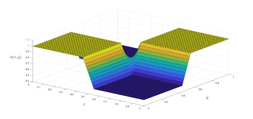
Figure 1: Surface of function $a(x,y)$ defined in Eq. 18.

The update function for inter-group bias is finally defined as:

$$\mu_{G}(\mathbf{x})=\mathbf{x}_{i}+\sum_{j\in A_{i}}\overline{I_{j,i}}\alpha_{ij}(\mathbf{x}_{i},\mathbf{x}_{j})(\mathbf{x}_{i}-\mathbf{x}_{j}),$$ (19)

where $\alpha_{ij}(\mathbf{x}_{i},\mathbf{x}_{j})=a(\mathbf{x}_{i},\mathbf{x}_{j})$.

The following example illustrates evolution of opinion under this form of inter-group bias.

Example 5.1.

Let $\left(G,\mathbf{x}^{0},\mu_{G}\right)$ be a generalized-bias model for six agents where $G$ is the graph in Figure 2(a). The initial state of opinion is $\mathbf{x}^{0}=\left[0.0,0.75,0.1,0.48,0.52,1.0\right]$ and $\mu_{G}$ is the inter-group bias update in Equation 19. Initially, there are two agents that are progressives (agents in red), two moderates (agents in green), and two conservatives (agents in blue). Note that $G$ is strongly connected. Because of the influence graph and the initial state opinions, there are interactions between agents of different groups, as well as in the same group. Figure 2(b) illustrates the evolution of opinion of the agents converging to consensus (around a moderate opinion) as predicted by the consensus result in Theorem 4.3.

(a) Influence graph for Example 5.1.

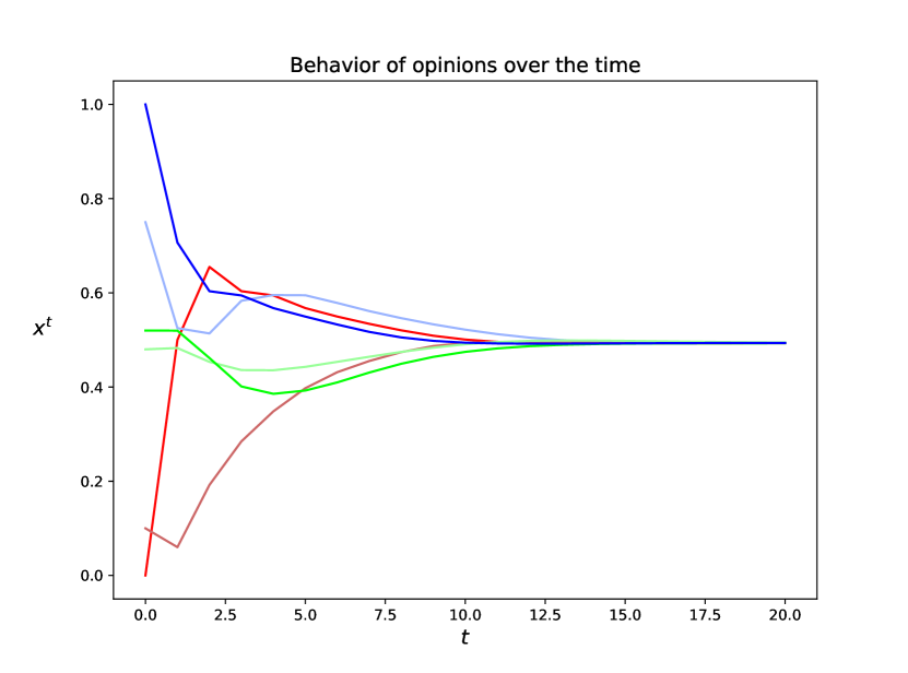
(b) Opinion evolution of the agents in Example 5.1. Each plot represents the evolution in time of the opinion of the agent in Fig. 2(a) with the same color.

Figure 2: Influence graph and opinion evolution.

6 Concluding Remarks

This paper introduced the notion of generalized-bias opinion dynamic model, a generalization of the classic DeGroot model, in which agents may react differently to the same opinion difference depending on whether the person holding the opposing view is from the same group. These reactions were formalized as arbitrary functions –parametric to the models– that depend, not only on opinion difference, but also on the opinions of the individuals interacting. This is a well-known bias in social psychology that cannot be modeled by state-of-the-art DeGroot-based models, as shown in Theorem 4.5. Furthermore, a consensus result was provided (Theorem 4.3), extending the classic result of the DeGroot model [9] for a wide range of social biases. Finally, an application example involving a particular case study of inter-group bias was used to illustrate the expressiveness of the new model.

The relevance of biased reasoning in human interactions has been extensively studied in [22], [18], [20], and others. Previous research in social psychology has explored intergroup bias [11, 10, 17], concluding that fostering dialogue between members of different groups reduces the disparity in their opinions. These findings align with the consensus results and the case study presented in the current work. The present model may bring further insights to social scientists about cognitive bias in opinion formation.

There is a great deal of work on formal models for belief change in social networks; we focus on the work on biased belief updates, which is the focus of this paper. Some models have previously been proposed to generalize the DeGroot model and introduce bias. For instance, [8], [7], and [23] analyze the effects of incorporating a bias factor for each agent to represent biased assimilation—how much of the external opinions the agent will take into consideration. The main difference between these models and the generalized-bias models in this paper is that in the previous models, biases are not represented as arbitrary continuous functions satisfying two conditions. Instead, biases are either modeled as an exponential factor that reduces the impact of neighbors’ opinions or by dynamically changing the weights in the DeGroot model with a specific function. Thus, the new model provides greater flexibility for capturing a wider range of biases.

The generalized-bias opinion models introduced here assume synchronous communication among the agents in the network, meaning all agents update their opinions simultaneously. In the line of [16, 3, 13], agents can also communicate asynchronously or via a hybrid blend where both types of communication can coexist. It would be interesting to see if the results presented here can be extended to these two settings. Moreover, it would be worth pursuing the use of rewriting logic to specify generalized-bias opinion models and perform several forms of formal analysis, including reachability analysis, model checking, and statistical model checking of concrete instances and desired properties of these models. Finally, the model could be extended to include agents that can learn by exchanging beliefs and lies as done in [13].

Appendix A Matrices and Dynamical Systems

A.1 Matrices

Square matrices in $\mathbb{R}^{N\times N}$ can be seen as representations of directed graphs with $N$ vertices and vice-versa.

Definition A.1.

The graph $G_{\mathbf{A}}$ associated to a matrix $\mathbf{A}=\left[a_{ij}\right]\in\mathbb{R}^{N\times N}$ is defined by $G_{\mathbf{A}}=(V_{\mathbf{A}},E_{\mathbf{A}})$ with $N$ nodes $V_{\mathbf{A}}=\{1,\ldots,N\}$ and edges $E_{\mathbf{A}}=\{(i,j)\mid a_{ij}=1\}$.

Structural properties of (square) matrices may be studied from the structure and connectivity in the associated graphs. Recall that a graph is strongly connected if it has exactly one strongly connected component (i.e., there is a path between any pair of its nodes).

Theorem A.2.

A matrix $\mathbf{A}$ is irreducible iff $G_{\mathbf{A}}$ is strongly connected.

Stochastic matrices are a special case of non-negative matrices. They are also known as a probability matrices, transition matrices, or Markov matrices, and are used to describe the transitions of a Markov chain.

Definition A.3.

A matrix $\mathbf{A}=\left[a_{ij}\right]\in\mathbb{R}^{N\times N}$ is called (right-)stochastic iff the following to conditions hold on $\mathbf{A}$:

1. It is non-negative.

2. The sum of each one of its rows is 1, i.e., for each $1\leq i\leq N$, it satisfies:

   $$\sum_{j=1}^{N}a_{ij}=1.$$

It can be checked that any stochastic matrix $\mathbf{A}$ has an eigenvalue equal to 1, which corresponds to its spectral radius. This follows from the fact that the sum of each row of $\mathbf{A}$ is 1, and hence there is an eigenvalue equal to 1 associated to a stationary distribution vector (i.e., a probability vector) $\mathbf{v}$ satisfying $\mathbf{A}\mathbf{v}=\mathbf{v}$.

A.2 Dynamical Systems

A dynamical system is a formal concept used to describe a system that evolves over time according to a specific set of rules.

Definition A.4.

A (discrete) dynamical system is a pair $\mathcal{S}=(S,\phi)$ where $S$ is a set and $\phi=\{\phi_{t}\}_{t\in T}$ is a family of $T$-indexed functions ${\phi_{t}}:{S}\longrightarrow{S}$, with $T$ a semigroup, satisfying for any $x\in S$ and $s,t\in T$:

1. $\phi_{0}(x)=x$.

2. $\phi_{s}(\phi_{t}(x))=\phi_{s+t}(x)$.

For convenience, the expression $\phi_{t}(x)$ is abbreviated $x_{t}$, for any $x\in S$ and $t\in T$.

In a dynamical system $\mathcal{S}=(S,\phi)$, the set $S$ represents all possible states of the system and the iterative application of $\phi$ defines the evolution of the system. The orbit of a state $x\in S$ is the set $\{x_{t}\mid t\in T\}$ of all states reachable from $x$. A set $\Lambda\subseteq S$ is called an invariant set of $\mathcal{S}$ iff $\phi_{t}(x)\in\Lambda$ for any $x\in\Lambda$ and $t\in T$. An invariant set is a subset of the state space that, once entered by a trajectory of the system, it cannot be left. In other words, if the system’s state ever enters an invariant set, it will remain in that set for all future time steps. Since an invariant set is a subset of the state space that is closed under transitions, it can include the orbits of many elements in the state space.

For the purpose of this work, the set $S$ is assumed to be $\mathbb{R}^{N}$ and the index set $T$ is the set of natural numbers $\mathbb{N}$.

Example A.5.

Consider the dynamical system $\mathcal{S}=(\mathbb{R}^{2},\phi)$, with $\phi=\{f^{n}\}_{n\in\mathbb{N}}$ and ${f}:{\mathbb{R}^{2}}\longrightarrow{\mathbb{R}^{2}}$ defined by:

$$f(\mathbf{x})=\mathbf{A}\mathbf{x}=\left[\begin{array}[]{lcc}0.5&0.5\\ 0.2&0.8\end{array}\right]\mathbf{x}.$$

Note that $f$ is the application of the irreducible stochastic matrix $\mathbf{A}$ on a given vector $\mathbf{x}$. By the Perron-Frobenius Theorem (see Section 2), the spectral radius $\rho(\mathbf{A})=1$ has multiplicity 1. Therefore, there is exactly one eigenvector $\mathbf{v}$ (modulo scalar multiplication) satisfying $\mathbf{x}=f(\mathbf{x})$. Consequently, the identity over $\mathbb{R}^{2}$ is an invariant set for $\mathcal{S}$.

An attractor in a dynamical system is an invariant set toward which the system tends to evolve from a wide variety of initial conditions. Attractors can play a crucial role in understanding the long-term behavior of dynamical systems.

Definition A.6.

Let $\mathcal{S}=(S,\phi)$ be a dynamical system. An attractor is a set of states $U\subseteq S$ with the following properties:

1. $U$ is an invariant set.

2. For any point $x\in U$, the distance from $x_{n}$ to $U$ tends to zero as $n\in\mathbb{N}$ tends to infinity.

Attractors can be fixed points, periodic orbits, limit cycles, or more complex structures like strange attractors. They are invariant and have a basin of attraction that draws nearby trajectories, making them key to understanding the system’s long-term behavior.

An $\omega$-limit set (often called an $\omega$-set) is a set of accumulation points that a trajectory approaches as time goes to infinity. It also provides important information about the long-term behavior of the system. Formally, for $\mathcal{S}=(S,\phi)$ a dynamical system, the $\omega$-limit set of a point $x\in S$, denoted $\omega(x)$, is defined as the set of all points $y\in S$, such that there exists an (strictly) increasing sequence $\{n_{k}\}_{k\in\mathbb{N}}$ satisfying $\lim_{k\to\infty}\phi_{n_{k}}(x)=y$.

Example A.7.

Consider the dynamical system $\mathcal{S}=([0..1],\phi)$, with $\phi=\{f^{n}\}_{n\in\mathbb{N}}$ and ${f}:{\mathbb{R}}\longrightarrow{\mathbb{R}}$ the logistic map defined by $f(x)=\mu x(1-x)$.

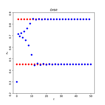
Figure 3: Orbit of point $x_{0}$ under map $L$, with $\mu=3.4$ in blue. Set $\left\{0.4519,0.8421\right\}$ in red.

Figure 3 depicts the orbit of $x_{0}$ in $\mathcal{S}$ when setting $\mu=3.4$ and $x_{0}=0.3$. It converges to the set $U=\left\{0.4519,0.8421\right\}$ (the red dots). The even indexes converge to $0.4519$ and the odd indexes converge to $0.8421$. That is, $\omega(x_{0})=U$.

Appendix B Proofs

In this appendix, we present the proofs of our theoretical results for consensus.

B.1 Lemma 4.1

To prove this result, we have to prove that for all $\mathbf{x}\in\left[0,1\right]^{N}$, the entries $a_{ij}(\mathbf{x})$ of matrix $\mathbf{A}(\mathbf{x})$, satisfy

• $a_{ij}(\mathbf{x})\geq 0$, for all $i,j=1,\ldots N$.

• $\sum^{N}_{j=1}a_{ij}(\mathbf{x})=1$, for all $i=1,\cdots N$.

We begin the proof with the definition of these entries, given in equation (7)

$$a_{i,j}(\mathbf{x})=\left\{\begin{array}[]{lcc}\vspace{0.5cm}1-\sum_{k\in A_{i}}\overline{I_{k,i}}\alpha_{i,k}(\mathbf{x})&\quad\mbox{, if}&i=j\\ \overline{I_{j,i}}\alpha_{i,j}(\mathbf{x})&\quad\mbox{, if}&i\neq j.\end{array}\right.$$ (22)

Note that $a_{i,i}=1-(a_{i,1}+\ldots a_{i,i-1}+a_{i,i+1}+\ldots a_{i,N})$, then, it is easy to see that $a_{i,1}+\ldots a_{i,i-1}+a_{i,i}+a_{i,i+1}+\ldots a_{i,N}=1$.

Now, note that $a_{i,j}\geq 0$, $i\neq j$, since $\overline{I}_{j,i}\geq 0$ and $\alpha_{i,j}(\mathbf{x})\geq 0$, for all $i,j=1,\ldots N$.

Recall that $\sum_{j\in A_{i}}\overline{I}_{j,i}=1$ and $\alpha_{i,j}(\mathbf{x})\leq 1$, furthermore, for each $i\in A$, there exist a neighbor $j\in A_{i}$ such that $\alpha_{i,j}(\mathbf{x})<1$, then

$$\sum^{N}_{k\in A_{i}}I_{k,i}\alpha_{i,k}(\mathbf{x})<\sum^{N}_{k\in A_{i}}I_{k,i}=1,$$

with this, we can check that $a_{i,i}=1-\sum^{N}_{k\in A_{i}}I_{k,i}\alpha_{i,k}(\mathbf{x})>0$.

Hence $\mathbf{A}(\mathbf{x})$ is stochastic, for all $\mathbf{x}\in\left[0,1\right]^{N}$.

B.2 Lemma 4.2

To prove that matrix $\mathbf{A}(\mathbf{x})$ is primitive, we have to check several conditions

• $\mathbf{A}(\mathbf{x})$ is irreducible for all $\mathbf{x}\in\left[0,1\right]^{N}$.

• There exists $m>0$, such that $\mathbf{A}^{m}(\mathbf{x})$, for all $\mathbf{x}\in\left[0,1\right]^{N}$.

By Theorem A.2, prove that for all $\mathbf{x}\in\left[0,1\right]^{N}$, $\mathbf{A}^{m}(\mathbf{x})$ is irreducible, is equivalent to prove that the graph $G_{\mathbf{A}(\mathbf{x})}$ associated at $\mathbf{A}(\mathbf{x})$, is strongly connected.

By hypothesis, the graph $G$, is strongly connected, then for each pair of vertex $i,j$, there exist a path of edges $(i,v_{2})\ldots(v_{k},j)$ which connects these vertex.

It is easy to see that $I_{j,i}>0$, implies $a_{i,j}>0$, for $i\neq j$. Then, for each edge $(j,i)$ in $E$, there exists an edge between vertex $(i,j)$, in $G_{\mathbf{A}(\mathbf{x})}$. From this, we can conclude that for each pair of vertex $(i,j)$ in $G_{\mathbf{A}(\mathbf{x})}$, exists a path of edges which connects these vertex, hence $G_{\mathbf{A}(\mathbf{x})}$ is strongly connected.

Above argument show that $\mathbf{A}(\mathbf{x})$ is irreducible for all $\mathbf{x}\in\left[0,1\right]^{N}$.

To prove the second condition, we shall use the Frobenius test of primitivity with $m=\left|A\right|$. If we denote $a^{(m)}_{i,j}$ like the entry $i,j$ of matrix $\mathbf{A}^{m}$, then we must prove that $a^{(m)}_{i,j}>0$, for all $i,j=1,\ldots N$.

We shall prove this with the next two claims

Claim 1: If exist a path of length $l$ between $i$ and $j$, then $a^{(l)}_{i,j}>0$.

Proof: We prove this claim by induction over $l$.

The base case is $l=1$, what is trivial, since the existence of an edge $(i,j)$ implies $a_{i,j}>0$.

Inductively, assume that if exist a path of length $l$ between 2 nodes $i$, $k$, then $a^{(l)}_{i,k}>0$.

Consider a pair of vertex $i$, $j$ and a path of edges $(i,v_{1})(v_{1},v_{2})\ldots(v_{l-1}.v_{l})(v_{l},j)$ of length $l+1$. For inductively hypothesis $a^{(l)}_{i,v_{l}}>0$, then

$$a^{(l+1)}_{i,j}=\sum^{N}_{k=1}a^{(l)}_{i,k}a_{k,j}\geq a^{(l)}_{i,v_{l}}a_{v_{l},j}>0.$$

It is proved.

Claim 2: If $a^{(n)}_{i,j}>0$, then $a^{(n+1)}_{i,j}>0$, for all $n\geq 1$.

Proof: Recall that for all $j=1,\ldots N$, $a_{j,j}>0$, then, if we have $a^{(n)}_{i,j}$, for some $n\geq 1$, we have

$$a^{(n+1)}_{i,j}=\sum^{N}_{k=1}a^{(n)}_{i,k}a_{k,j}\geq a^{(n)}_{i,j}a_{j,j}>0.$$

It is proved.

Since for all $\mathbf{x}\in\left[0,1\right]^{N}$, $G_{\mathbf{A}(\mathbf{x})}$ is strongly connected, then for each pair of vertex $(i,j)$ exists a path of length $l$, where $l\leq\left|A\right|$. By Claim 1, $a^{(l)}_{i,j}>0$, and by Claim 2, $a^{(\left|A\right|)}_{i,j}>0$. Then $\mathbf{A}^{\left|A\right|}(\mathbf{x})>0$, and by Frobenius test of primitivity, $\mathbf{A}(\mathbf{x})$ is primitive.

B.3 Theorem 4.3

The proof of this result requires several concepts from dynamical systems, as well as the lemmas stated above. Recall that an update function converges to consensus if there exists a $v\in\left[0,1\right]$ such that, for every agent $i\in A$, their opinion $\mathbf{x}^{t}_{i}$ satisfies $\lim_{t}\mathbf{x}^{t}_{i}=v$.

We equivalently prove that the sequence $\left\{\eta_{k}\right\}\subset\mathbb{R}$, defined by $\eta_{k}=\left\lVert\mathbf{x}^{k}-\overline{\mathbf{x}^{k}}\right\rVert$, where $\mathbf{x}^{k+1}=\mu_{G}(\mathbf{x}^{k})$, converges at $\eta_{k}\to 0$.

Proof is composed of the next way

• Prove that the sequence $\eta_{k}=\left\lVert\mathbf{x}^{k}-\overline{\mathbf{x}}_{k}\right\rVert$ converges at one value $L\geq 0$ when $k\to\infty$.

• Prove that $L=0$.

Consider the line $l\subset\mathbb{R}^{N}$, defined by $l=\left\{r\mathbf{1}:r\in\mathbb{R}\right\}$, where 1 is a vector whose all entries are equal to 1.

Claim 1: The point $\mathbf{y}=\overline{\mathbf{x}}\in l$, is the point who minimize the distance $\left\lVert\mathbf{x}-\textbf{y}\right\rVert$.

Proof: Proof of above claim is a geometric property, since $\overline{\mathbf{x}}$ is the projection of $\mathbf{x}$ over the line $l$.

Claim 2: The sequence $\eta_{k}=\left\lVert\mathbf{x}^{k}-\overline{\mathbf{x}^{k}}\right\rVert$, where $\mathbf{x}^{k+1}=\mu_{G}(\mathbf{x}^{k})$, converges at converges at one value $L\geq 0$.

Proof: To prove this claim, we have to prove that the sequence $\eta_{k}$ is monotonous and bounded.

First, we use the Claim 1 and that vectors in $l$ are fixed points of map $F$

$$\begin{split}\left\lVert\mathbf{x}^{k+1}-\overline{\mathbf{x}^{k+1}}\right\rVert&<\left\lVert\mathbf{x}^{k+1}-\overline{\mathbf{x}^{k}}\right\rVert,\\ \left\lVert\mathbf{x}^{k+1}-\overline{\mathbf{x}^{k+1}}\right\rVert&<\left\lVert\mathbf{A}(\mathbf{x}^{k})\mathbf{x}^{k}-\mathbf{A}(\mathbf{x}^{k})\overline{\mathbf{x}^{k}}\right\rVert,\\ \left\lVert\mathbf{x}^{k+1}-\overline{\mathbf{x}^{k+1}}\right\rVert&<\left\lVert\mathbf{A}(\mathbf{x}^{k})\right\rVert\left\lVert\mathbf{x}^{k}-\overline{\mathbf{x}^{k}}\right\rVert,\\ \end{split}$$

Vector $\mathbf{x}^{k}-\overline{\mathbf{x}^{k}}$ is in the space generated by the eigenvectors $\mathbf{v}_{2},\ldots\mathbf{v}_{s}$, $s\geq N$. This space is invariant for the operator $\mathbf{A}$, then the norm of this operator is $\left|\lambda_{2}\right|<1$ (because $\mathbf{A}$ is primitive), then

$$\begin{split}\left\lVert\mathbf{x}^{k+1}-\overline{\mathbf{x}^{k+1}}\right\rVert&<\left|\lambda_{2}\right|\left\lVert\mathbf{x}^{k}-\overline{\mathbf{x}^{k}}\right\rVert,\\ \left\lVert\mathbf{x}^{k+1}-\overline{\mathbf{x}^{k+1}}\right\rVert&<\left\lVert\mathbf{x}^{k}-\overline{\mathbf{x}^{k}}\right\rVert,\\ \end{split}$$

With this, we have shown that the sequence is decreasing monotone.

By properties of the norm operator $\left\lVert.\right\rVert$, this is non negative, for this reason and the monotonic property, the sequence is bounded. For each $k\geq 1$, we have $0\leq\eta_{k}\leq\eta_{0}$. By the real analysis, we know that this sequence converges at some value $L$, where $0\leq L\leq\eta_{0}$.

Claim 3: The limit $L$ of the sequence $\eta_{k}$ is $L=0$.

The first item to prove this claim, is that the update function $\mu_{G}$ defined in (4) is continuous. We know this because this map is composed by continuous functions.

For properties of continuous dynamical systems presented in Appendix A.2, we have that for each initial condition $\mathbf{x}^{0}$, the set $\omega_{F}(\mathbf{x}^{0})$ is an invariant set; which means that for all $\textbf{y}\in\omega_{F}(\mathbf{x}^{0})$, $F(\textbf{y})\in\omega_{F}(\mathbf{x}^{0})$.

Now, let us proceed by contradiction. Suppose that $L>0$, then $\left\lVert\mathbf{x}^{k}-\overline{\mathbf{x}^{k}}\right\rVert\to L>0$, when $k\to\infty$. This implies that $\omega_{\mu}(\mathbf{x}^{0})$ is a subset of the sphere of radius $L$ centered in a point $\mathbf{p}\in\mathbb{R}^{N}$ of the line $l$, denoted by $S_{L}$.

Let $\mathbf{y}\in\omega_{\mu}(\mathbf{x}^{0})$, by our above reasoning, we have that $\left\lVert\mathbf{y}-\overline{\mathbf{y}}\right\rVert>\left\lVert\mu_{G}(\mathbf{y})-\overline{\mu_{G}(\mathbf{y})}\right\rVert$, but this contradicts the invariance of $\omega_{\mu_{G}}(\mathbf{x}^{0})$, because the distance of $F(\mathbf{y})$ is less than $L$.

In conclusion, $L$ must be equal to zero.

References

- [1] M. S. Alvim, B. Amorim, S. Knight, S. Quintero, and F. Valencia. A formal model for polarization under confirmation bias in social networks. LMCS, 2023.
- [2] M. S. Alvim, A. G. da Silva, S. Knight, and F. Valencia. A multi-agent model for opinion evolution in social networks under cognitive biases. In Formal Techniques for Distributed Objects, Components, and Systems,, volume 14678 of LNCS, pages 3–19. Springer, 2024.
- [3] J. Aranda, S. Betancourt, J. F. Díaz, and F. Valencia. Fairness and consensus in an asynchronous opinion model for social networks. In 35th International Conference on Concurrency Theory, CONCUR. Schloss Dagstuhl - Leibniz-Zentrum für Informatik, 2024.
- [4] E. Aronson, T. Wilson, and R. Akert. Social Psychology. Upper Saddle River, NJ : Prentice Hall, 7 edition, 2010.
- [5] M. Bernardo, C.J.Budd, A.R.Champneys, and P.Kowalczyk. Piecewise-smooth Dynamical Systems Theory and Applications. Springer Science, 2008.
- [6] A. G. Chandrasekhar, H. Larreguy, and J. P. Xandri. Testing models of social learning on networks: Evidence from a lab experiment in the field. Working Paper 21468, National Bureau of Economic Research, August 2015.
- [7] Z. Chen, J. Qin, B. Li, H. Qi, P. Buchhorn, and G. Shi. Dynamics of opinions with social biases. Automatica, 106:374–383, 2019.
- [8] P. Dandekar, A. Goel, and D. Lee. Biased assimilation, homophily and the dynamics of polarization. Proceedings of the National Academy of Sciences of the United States of America, 110, 03 2013.
- [9] M. H. DeGroot. Reaching a consensus. Journal of the American Statistical association, 69(345):118–121, 1974.
- [10] S. L. Gaertner and J. F. Dovidio. Reducing intergroup bias: The common ingroup identity model. Psychology Press, 2014.
- [11] S. L. Gaertner, J. F. Dovidio, M. C. Rust, J. A. Nier, B. S. Banker, C. M. Ward, G. R. Mottola, and M. Houlette. Reducing intergroup bias: elements of intergroup cooperation. Journal of personality and social psychology, 76(3):388, 1999.
- [12] B. Golub and E. Sadler. Learning in social networks. Available at SSRN 2919146, 2017.
- [13] S. Haar, S. Perchy, C. Rueda, and F. Valencia. An algebraic view of space/belief and extrusion/utterance for concurrency/epistemic logic. In 17th International Symposium on Principles and Practice of Declarative Programming (PPDP 2015), 2015.
- [14] M. Hewstone, M. Rubin, and H. Willis. Intergroup bias. Annual review of psychology, 53(1):575–604, 2002.
- [15] C. D. Meyer. Matrix Analisys and Applied Linear Algebra. SIAM, 2000.
- [16] C. Olarte, C. Ramírez, C. Rocha, and F. Valencia. Unified opinion dynamic modeling as concurrent set relations in rewriting logic. In 15th International Workshop, WRLA, Revised Selected Papers. Springer, 2024.
- [17] T. F. Pettigrew and L. R. Tropp. How does intergroup contact reduce prejudice? meta-analytic tests of three mediators. European journal of social psychology, 38(6), 2008.
- [18] V. J. Ramos. Analyzing the role of cognitive biases in the decision-making process. Advances in Psychology, Mental Health, and Behavioral Studies, 2018.
- [19] H. Tajfel. An integrative theory of intergroup conflict. The social psychology of intergroup relations/Brooks/Cole, 1979.
- [20] B. M. Tappin and S. Gadsby. Biased belief in the bayesian brain: A deeper look at the evidence. Consciousness and Cognition, 68:107–114, 2019.
- [21] S. Wasserman and K. Faust. Social network analysis in the social and behavioral sciences. In Social Network Analysis: Methods and Applications. Cambridge University Press, 1994.
- [22] D. Williams. Hierarchical bayesian models of delusion. Consciousness and Cognition, 61:129–147, 2018.
- [23] W. Xia, M. Ye, J. Liu, M. Cao, and X.-M. Sun. Analysis of a nonlinear opinion dynamics model with biased assimilation. Automatica, 120:109113, 2020.