Partial Distribution Matching via
Partial Wasserstein Adversarial Networks

Abstract

This paper studies the problem of distribution matching (DM), which is a fundamental machine learning problem seeking to robustly align two probability distributions. Our approach is established on a relaxed formulation, called partial distribution matching (PDM), which seeks to match a fraction of the distributions instead of matching them completely. We theoretically derive the Kantorovich-Rubinstein duality for the partial Wasserstain-$1$ (PW) discrepancy, and develop a partial Wasserstein adversarial network (PWAN) that efficiently approximates the PW discrepancy based on this dual form. Partial matching can then be achieved by optimizing the network using gradient descent. Two practical tasks, point set registration and partial domain adaptation are investigated, where the goals are to partially match distributions in 3D space and high-dimensional feature space respectively. The experiment results confirm that the proposed PWAN effectively produces highly robust matching results, performing better or on par with the state-of-the-art methods.

1 Introduction

Distribution matching (DM) is a fundamental machine learning task with many applications. As illustrated in Fig. 1(a), given two probability distributions, the goal of DM is to match one distribution to the other. For example, in generative modelling, to describe the observed data, a parametric model distribution is matched to the data distribution. Recently advanced DM algorithms [1, 2, 3] are well known for being able to handle highly complicated distributions. However, these methods still have difficulty handling distributions that are contaminated by outliers, because their attempt to completely match the “dirty” distributions will inevitably lead to biased results.

A natural way to address this issue is to consider the partial distribution matching (PDM) task as a relaxation of the DM task: given two unnormalized distributions of mass, i.e., the total mass of each distribution is not necessarily $1$, the goal of PDM is to match a certain fraction of mass of the two distributions. An example of PDM is presented in Fig. 1(b). In contrast to DM, PDM allows to omit the fraction of distribution that does not match, thus it naturally tolerates outliers better. In other words, it is more suitable for applications with dirty data.

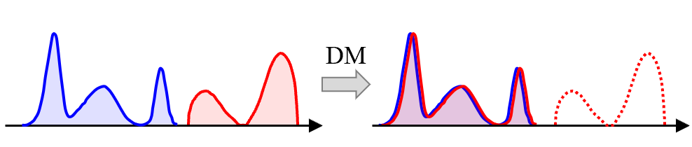
(a) Given two normalized distributions, DM aims to match the source distribution (red) to the reference distribution (blue).

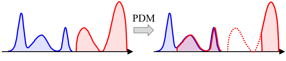
(b) Given two unnormalized distributions, PDM aims to match a certain fraction of the source distribution (red) to the reference distribution (blue).

Figure 1: Comparison between DM and PDM. DM aims to completely match two distributions, but PDM only aims to match a certain fraction of them.

Several PDM methods have been investigated, but they tend to be computationally expensive for large-scale PDM problems, because they generally rely on the correspondence between distributions [4, 5, 6]. To address this issue, we propose an efficient PDM algorithm, called partial Wasserstein adversarial network (PWAN), based on deep neural networks and the optimal transport (OT) theory [7]. Our key idea is to partially match the distributions by minimizing their partial Wasserstein-1 (PW) discrepancy [8] which is approximated by a neural network. Specifically, we first derive the Kantorovich-Rubinstein (KR) dual form [9] for the PW discrepancy, and show that its gradient can be explicitly computed via its potential. These results then allow us to compute the PW discrepancy by approximating the potential using a deep neural network, and minimize it by gradient descent. Compared to the existing PDM methods, the proposed PWAN is correspondence-free, thus it is more efficient for large-scale PDM tasks. In addition, PWAN is a direct generalization of the well-known DM algorithm Wasserstein GAN (WGAN) [1] for PDM tasks.

To show the effectiveness of the proposed PWAN, we apply it to two practical tasks: point set registration [10] and partial domain adaptation [11, 12], where PWAN is used to match distributions in 3D space and high dimensional feature space respectively. Specifically, point set registration [10] seeks to align two point sets representing incomplete shapes in 3D space. We regard point sets as discrete distributions, then the registration problem can be naturally formulated as a PDM problem. On the other hand, the goal of partial domain adaptation is to train a classifier for the test data under the assumption that the test and training data are sampled from different domains, and the test label set is a subset of the training label set. We formulate the adaptation problem as a PDM problem, where we seek to align the test feature distribution to a fraction of the training feature distribution, so that the classifier learned for the training set can be readily used for the test set.

These two PDM tasks have two common challenges: 1) they involve large-scale distributions, such as point sets consisting of $10^{5}$ points, or large-scale image datasets, and 2) the distributions may be dominated by outliers, e.g., the outlier ratio can be up to $90\%$ in partial adaptation tasks. Thanks to its efficient formulation and partial matching principle, PWAN can naturally address these two difficulties. The experiment results confirm that PWAN can produce highly robust matching results, and it performs better than or is at least comparable with the state-of-the-art methods.

In summary, the contributions of this work are:

• Theoretically, we derive the Kantorovich-Rubinstein (KR) duality of the partial Wasserstein-1 (PW) discrepancy. We further study its differentiability and present a qualitative description of the solution to the KR dual form.

• Based on the theoretical results, we propose a novel algorithm, called Partial Wasserstein Adversarial Network (PWAN), for partial distribution matching (PDM). PWAN approximates distance-type or mass-type PW divergences by neural networks, thus it can be efficiently trained using gradient descent. Notably, PWAN is a generalization of the well-known Wasserstein GAN.

• We apply PWAN to point set registration, where we partially align discrete distributions representing point sets in 3D space. We evaluate PWAN on both non-rigid and rigid point set registration tasks, and show that PWAN exhibits strong robustness against outliers, and can register point sets accurately even when they are dominated by noise points or are only partially overlapped.

• We apply PWAN to partial domain adaptation, where we align the test feature distribution to a fraction of the training feature distribution . We evaluate PWAN on four benchmark datasets, and show that it can effectively avoid biased results even with high outlier ratio.

The rest of this work is organized as follows: Sec. 2 reviews some related works. Sec. 3 recalls the definitions of PW divergences which are the major tools used in PWAN. Sec. 4 derives the formulation of PWAN, and provides a concrete training algorithm. Some connections between PWAN and WGAN are also discussed. Sec. 5 applies PWAN to point set registration, and Sec. 6 applies PWAN to partial domain adaptation. Sec. 7 finally draws some conclusions.

This work extends our earlier work [13] in the following ways:

• We complete the point set registration experiments by applying PWAN to rigid registration tasks.

• To demonstrate the ability of PWAN in matching distributions in high dimensional feature space, we apply PWAN to partial domain adaptation tasks. We provide a concrete algorithm for partial domain adaptation, and experimentally demonstrate its effectiveness.

2 Related Works

PWAN is developed based on OT theory [7, 8, 14], which is a powerful tool for comparing distributions. Various types of numerical OT solvers have been proposed [15, 6, 16, 5, 17, 18]. A well-known type of solver is the entropy-regularized solver [19, 20, 4], which iteratively estimates the transport plan, i.e., the correspondence, between distributions. This type of solver is flexible as it can handle a wide range of cost functions [7], but it is generally computationally expensive for large-scale distributions. Some efficient mini-batch-based approximations [21, 22] have been proposed to alleviate this issue, but these methods are known to suffer from mini-batch errors, thus extra modifications are usually needed [23].

PWAN belongs to the Wasserstein-1-type OT solver, which is dedicated to the special OT problem where the cost function is a metric. This type of solver exploits the KR duality of the Wasserstein-1-type metrics, thus it is generally highly efficient. A representative method in this class is WGAN [1], which approximates the Wasserstein-1 distance using neural networks. PWAN is a direct generalization of WGAN, because it approximates the PW divergence, which is a generalization of the Wasserstein-1 distance, under the same principle as WGAN. In addition, [24, 18] studied the KR duality of various Wasserstein-1-type divergences, including the distance-type PW divergence considered in this work. Our work completes these works [24, 18] in the sense that we additionally study the mass-type PW divergence, and we provide a continuous approximation of PW discrepancies using neural networks, which is suitable for a broad range of applications.

Point set registration is a classic PDM task that seeks to match discrete distributions, i.e., point sets. This task has been extensively studied for decades, and various methods have been proposed [25, 26, 27, 10, 28, 29, 30]. PWAN is related to the probabilistic registration methods, which solve the registration task as a DM problem. Specifically, these methods first smooth the point sets as Gaussian mixture models (GMMs), and then align the distributions via minimizing the robust discrepancies between them. Coherent point drift (CPD) [10] and its variants [30] are well-known examples in this class, which minimize Kullback-Leibler (KL) divergence between the distributions. Other robust discrepancies, including $L_{2}$ distance [31, 32], kernel density estimator [33] and scaled Geman-McClure estimator [34] have also been studied.

The proposed PWAN has two major differences from the existing probabilistic registration methods. First, it directly processes the point sets as discrete distributions instead of smoothing them to GMMs, thus it is more concise and natural. Second, it solves a PDM problem instead of a DM problem, as it only requires matching a fraction of points, thus it is more robust to outliers.

Recently, some works have been devoted to a new PDM task, i.e., partial domain adaptation [12, 11, 35], where the goal is to partially match two feature distributions. This task was first formally addressed by [12], where a re-weighting procedure was used to discard a fraction of the distributions as outliers, and a DM model was then used to align the rest of the distributions. Other DM methods, such as maximum mean discrepancy network [36], and more advanced re-weighting procedures [37, 38, 11] have been studied. To eliminate the need for re-weighting procedures, the mini-batch OT solver [21, 23] has been investigated.

The proposed PWAN is conceptually close to the existing mini-batch-OT-based methods [21, 23] because they are based on the OT theory. However, in contrast to these methods, PWAN does not suffer from mini-batch errors [23], because it performs PDM for the whole data distributions instead of the mini-batched samples. In addition, the GAN-based adaptation methods [39, 40] can be seen as a special case of the proposed PWAN, where the data does not contain outliers.

3 Preliminaries on PW Divergences

This section introduces the major tools used in this work, i.e., two types of PW divergences: the partial-mass Wasserstein-1 discrepancy [8, 14] and the bounded-distance Wasserstein-1 discrepancy [24, 41]. We refer readers to [7] for a more complete introduction to the OT theory.

Let $\alpha,\beta\in\mathcal{M}_{+}(\Omega)$ be the reference and the source distribution of mass, where $\Omega$ is a compact metric space, and $\mathcal{M}_{+}(\Omega)$ is the set of non-negative measures defined on $\Omega$. Denote $m_{\beta}=\beta(\Omega)$ and $m_{\alpha}=\alpha(\Omega)$ the total mass of $\beta$ and $\alpha$ respectively. The partial-mass Wasserstein-1 discrepancy $\mathcal{L}_{M,m}(\alpha,\beta)$ is defined as

$$\mathcal{L}_{M,m}(\alpha,\beta)=\inf_{\pi\in\Gamma_{m}(\alpha,\beta)}\int_{\Omega\times\Omega}{\bm{d}}(x,y)d\pi(x,y),$$ (1)

where $\Gamma_{m}(\alpha,\beta)$ is the set of $\pi\in\mathcal{M}_{+}(\Omega\times\Omega)$ satisfying

$$\pi(A\times\Omega)\leq\alpha(A),\quad\pi(\Omega\times A)\leq\beta(A)\quad and\quad\pi(\Omega\times\Omega)\geq m$$

for all measurable set $A\subseteq\Omega$ and ${\bm{d}}$ is the metric in $\Omega$.

In the complete OT case, i.e., $m=m_{\beta}=m_{\alpha}$, $\mathcal{L}_{M,m}$ is the Wasserstein-$1$ metric $\mathcal{W}_{1}$, which is also called the earth mover’s distance. According to the Kantorovich-Rubinstein (KR) duality [42], $\mathcal{W}_{1}$ can be equivalently expressed as

$$\mathcal{W}_{1}(\alpha,\beta)=\sup_{{\bm{f}}\in Lip(\Omega)}\int_{\Omega}{\bm{f}}d\alpha-\int_{\Omega}{\bm{f}}d\beta.$$ (2)

where $Lip(\Omega)$ represents the set of Lipschitz-1 functions defined on $\Omega$. (2) is exploited in WGAN [1] to efficiently compute $\mathcal{W}_{1}$, where ${\bm{f}}$ is approximated by a neural network.

Several methods have been proposed to generalize (2) to unbalanced OT [4, 16]. A unified framework of these approaches can be found in [18]. Amongst these generalizations, we considered the bounded-distance Wasserstein-1 discrepancy $\mathcal{L}_{D,h}$, which can be regarded as (1) with a soft mass constraint:

$$\mathcal{L}_{D,h}(\alpha,\beta)=\inf_{\pi\in\Gamma_{0}(\alpha,\beta)}\int_{\Omega\times\Omega}{\bm{d}}(x,y)d\pi(x,y)-hm(\pi).$$ (3)

Note that $\mathcal{L}_{D,h}$ can be interpreted as finding an optimal plan $\pi$ with a distance threshold $h$. Importantly, $\mathcal{L}_{D,h}$ is known to have an equivalent form [24, 18]

$$\mathcal{L}_{D,h}(\alpha,\beta)=\sup_{\begin{subarray}{c}{\bm{f}}\in Lip(\Omega)\\ -h\leq{\bm{f}}\leq 0\end{subarray}}\int_{\Omega}{\bm{f}}d\alpha-\int_{\Omega}{\bm{f}}d\beta-hm_{\beta}.$$ (4)

We call (2) and (4) KR forms, and the solution to KR forms potentials.

4 The Proposed Method

We present the details of the proposed PWAN in this section. We first formulate the PDM problem in Sec. 4.1. Then we present an efficient approach for the problem in Sec. 4.2 and 4.3. We finally discuss the connections between PWAN and the well-known WGAN [1] in Sec. 4.4 to provide a deeper understanding of PWAN.

4.1 Problem Formulation

Let $\alpha\in\mathcal{M}_{+}(\Omega)$, $\beta\in\mathcal{M}_{+}(\Omega^{\prime})$ be the reference and the source distribution of mass, where $\Omega^{\prime}$ and $\Omega$ are two compact subsets of Euclidean spaces. Let $\mathcal{T}_{\theta}:\Omega^{\prime}\rightarrow\Omega$ denote a differentiable transformation parametrized by $\theta$, and $\beta_{\theta}=(\mathcal{T}_{\theta})_{\#}\beta\in\mathcal{M}_{+}(\Omega)$ denote the push-forward of $\beta$ by $\mathcal{T}_{\theta}$. Our goal is to partially match $\beta_{\theta}$ to $\alpha$ by solving

$$\min_{\theta}\mathcal{L}(\alpha,\beta_{\theta})+\mathcal{C}(\theta),$$ (5)

where $\mathcal{L}$ represents $\mathcal{L}_{M,m}$ or $\mathcal{L}_{D,h}$, which measures the dissimilarity between $\beta_{\theta}$ and $\alpha$, and $\mathcal{C}$ is a differentiable regularizer that reduces the ambiguity of solutions.

4.2 Partial Matching via PW Divergences

To see the effectiveness of framework (5), we present a toy example of matching discrete distributions in Fig. 2. Let $Y=\{y_{j}\}_{j=1}^{r}$ and $X=\{x_{i}\}_{i=1}^{q}$ be the source and reference 2-D point sets, $\beta=\sum_{y_{j}\in Y}\delta_{y_{j}}$ and $\alpha=\sum_{x_{i}\in X}\delta_{x_{i}}$ be the corresponding discrete distributions, where $\delta$ is the Dirac function. We seek to find a transformation $\mathcal{T}_{\theta}$ that partially matches $Y$ to $X$ by solving (5).

By expressing $\mathcal{L}_{M,m}$ (1) and $\mathcal{L}_{D,h}$ (3) in their primal forms, we can write (5) as

$$\min_{\theta}\sum_{i,j}\pi_{ij}{\bm{d}}(x_{i},\mathcal{T}_{\theta}(y_{j}))+\mathcal{C}(\theta)+const,$$ (6)

where $const$ is a constant that is not related to $\theta$, and $\pi\in\mathbb{R}^{q\times r}$ is the solution to (1) or (3) obtained via linear programming. We represent the non-zero elements in $\pi$ by line segments in Fig. 2. As can be seen, the value of (6) only depends on the distances between the corresponding point pairs that are within the mass or distance threshold, thus minimizing (6) will only align these point pairs subjecting to the regularizer $\mathcal{C}$, while omitting all other points, i.e., the hollow points. In other words, $\mathcal{L}_{M,m}$ and $\mathcal{L}_{D,h}$ provide two ways to control the degree of alignment of distributions based on the mass or distance criteria.

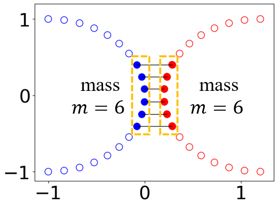
(a) $\mathcal{L}_{M,6}$

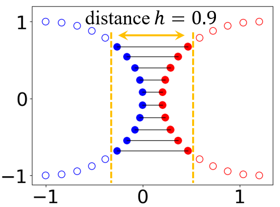
(b) $\mathcal{L}_{D,0.9}$

Figure 2: The computed correspondence $\pi$ between $\alpha$ (blue) and $\beta_{\theta}$ (red).

However, although the solution to (6) indeed partially matches the distributions, it is intractable for large-scale discrete distributions or continuous distributions, due to the high computational cost of solving for $\pi$ using a linear program in each iteration.

To address this challenge, we propose to avoid computing $\pi$ by optimizing $\mathcal{L}_{D,h}$ or $\mathcal{L}_{M,m}$ in their KR forms as an alternative to their primal forms. To this end, we first present the KR forms for $\mathcal{L}_{D,h}$ and $\mathcal{L}_{M,m}$, and then show that they are differentiable. As for $\mathcal{L}_{D,h}$, the KR form is known in (4), and we further show that it is valid to compute its gradient. We also show that a similar statement for $\mathcal{L}_{M,m}$ holds. Specifically, we have the following two theorems:

Theorem 1.

$\mathcal{L}_{D,h}(\alpha,\beta)$ can be equivalently expressed as (4). There is a solution ${\bm{f}}^{*}:\Omega\rightarrow\mathbb{R}$ to problem (4). If $\mathcal{T}_{\theta}$ satisfies a mild assumption, then $\mathcal{L}_{D,h}(\alpha,\beta_{\theta})$ is continuous w.r.t. $\theta$, and is differentiable almost everywhere. Furthermore, we have

$$\nabla_{\theta}\mathcal{L}_{D,h}(\alpha,\beta_{\theta})=-\int_{\Omega}\nabla_{\theta}({\bm{f}}^{*}\circ\mathcal{T}_{\theta})d\beta$$ (7)

when both sides are well-defined.

Theorem 2.

$\mathcal{L}_{M,m}(\alpha,\beta)$ can be equivalently expressed as

$$\mathcal{L}_{M,m}(\alpha,\beta)=\sup_{\begin{subarray}{c}{\bm{f}}\in Lip(\Omega),h\in\mathbb{R}_{+}\\ -h\leq{\bm{f}}\leq 0\end{subarray}}\int_{\Omega}{\bm{f}}d(\alpha-\beta)+h(m-m_{\beta}).$$ (8)

There is a solution ${\bm{f}}^{*}:\Omega\rightarrow\mathbb{R}$ to problem (8). If $\mathcal{T}_{\theta}$ satisfies a mild assumption, then $\mathcal{L}_{M,m}(\alpha,\beta_{\theta})$ is continuous w.r.t. $\theta$, and is differentiable almost everywhere. Furthermore, we have

$$\nabla_{\theta}\mathcal{L}_{M,m}(\alpha,\beta_{\theta})=-\int_{\Omega}\nabla_{\theta}({\bm{f}}^{*}\circ\mathcal{T}_{\theta})d\beta$$ (9)

when both sides are well-defined.

Theorem 1 and 2 immediately allow us to approximate $\mathcal{L}_{D,h}$ or $\mathcal{L}_{M,m}$ using neural networks. Specifically, let ${\bm{f}}_{w,h}$ be a neural network satisfying $-h\leq{\bm{f}}_{w,h}\leq 0$ and $\|\nabla{\bm{f}}_{w,h}\|\leq 1$, where $w$ and $h\in\mathbb{R}_{+}$ are parameters of the network ${\bm{f}}_{w,h}$, and $\|\nabla{\bm{f}}_{w,h}\|$ is the gradient of ${\bm{f}}$ w.r.t. the input. We can compute $\mathcal{L}_{M,m}(\alpha,\beta_{\theta})$ and $\mathcal{L}_{D,h}(\alpha,\beta_{\theta})$ according to (4) and (8):

$$\mathcal{L}_{M,m}(\alpha,\beta_{\theta})=\max_{w,h}\int_{\Omega}{\bm{f}}_{w,h}d\alpha- \int_{\Omega}({\bm{f}}_{w,h}\circ\mathcal{T}_{\theta})d\beta$$

$$+h(m-m_{\beta}),$$ (10)

and

$$\mathcal{L}_{D,h}(\alpha,\beta_{\theta})=\max_{w}\int_{\Omega}{\bm{f}}_{w,h}d\alpha-\int_{\Omega}({\bm{f}}_{w,h}\circ\mathcal{T}_{\theta})d\beta-hm_{\beta}$$ (11)

using gradient descent and back-propagation.

Using the approximated KR forms of $\mathcal{L}_{M,m}$ (4.2) and $\mathcal{L}_{M,m}$ (11), we can finally rewrite (5) as

$$\min_{\theta}\bigl{(}-{\bm{f}}_{w,h}^{*}(\mathcal{T}_{\theta}(y_{j}))+\mathcal{C}(\theta)+const\bigr{)},$$ (12)

where ${\bm{f}}_{w,h}^{*}$ is the solution to $\mathcal{L}_{M,m}$ (4.2) or $\mathcal{L}_{D,h}$ (11). To see the connection between this KR-based formulation (12) and the primal formulation (6), we present an example in Fig. 3. In contrast to (6), which matches a fraction of $\beta_{\theta}$ to the corresponding points in $\alpha$ (1-st row), (12) is correspondence-free, and it seeks to move $\beta_{\theta}$ along the direction of $\nabla{\bm{f}}_{w,h}^{*}$. Note that the points with zero gradients (hollow points in the 3-rd row) are omitted by (12), and the same group of points (hollow points in the 1-st row) are also omitted by (6), which indicates the consistency of these two formulations. Further numerical results in Appx. B.1 confirm that these two forms are indeed consistent. More discussions of the property of the potential are presented in Sec. 4.4 and Appx. A.2.

$\pi$
${\bm{f}}^{*}$
$||\nabla{\bm{f}}^{*}||$

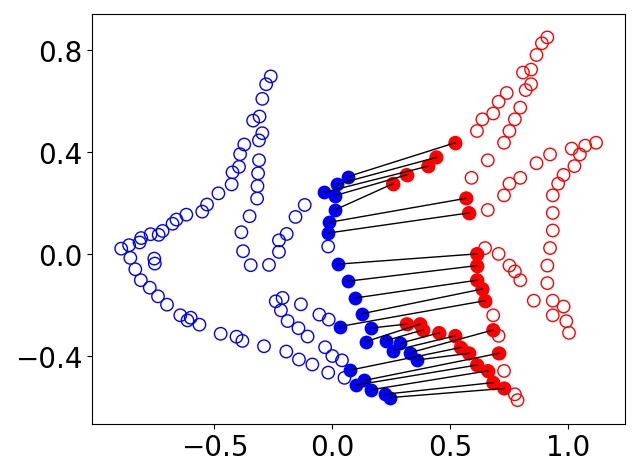
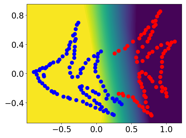
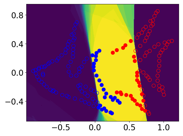
(a) $\mathcal{L}_{M,25}$ or $\mathcal{L}_{D,0.64}$

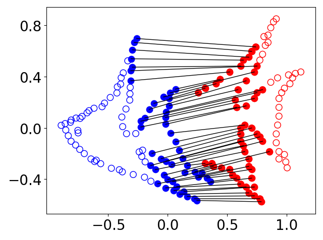
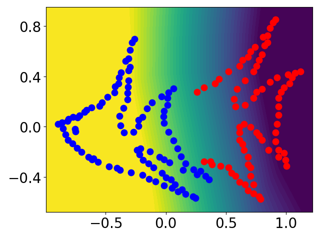
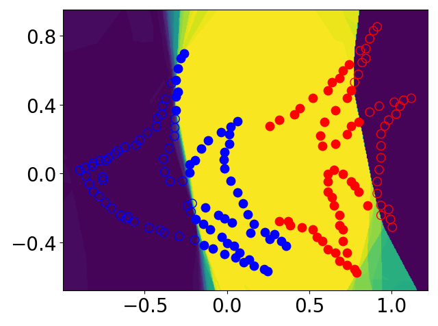
(b) $\mathcal{L}_{M,50}$ or $\mathcal{L}_{D,1.09}$

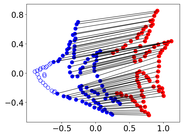
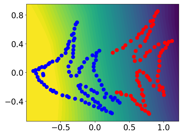
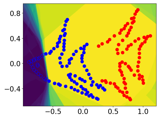
(c) $\mathcal{L}_{M,78}$ or $\mathcal{L}_{D,5}$

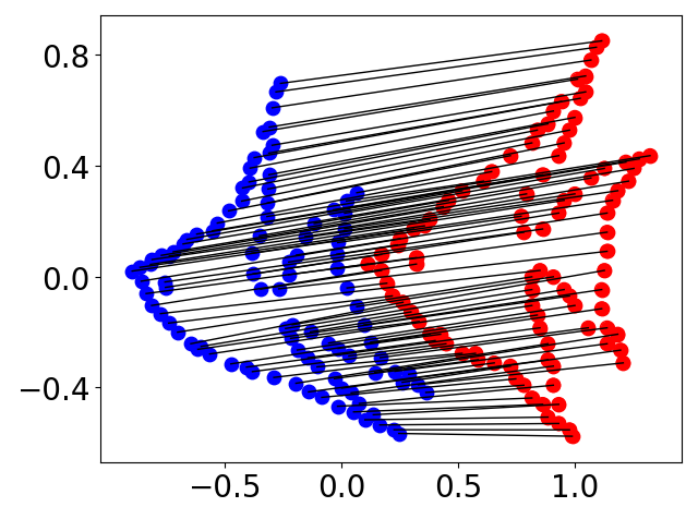
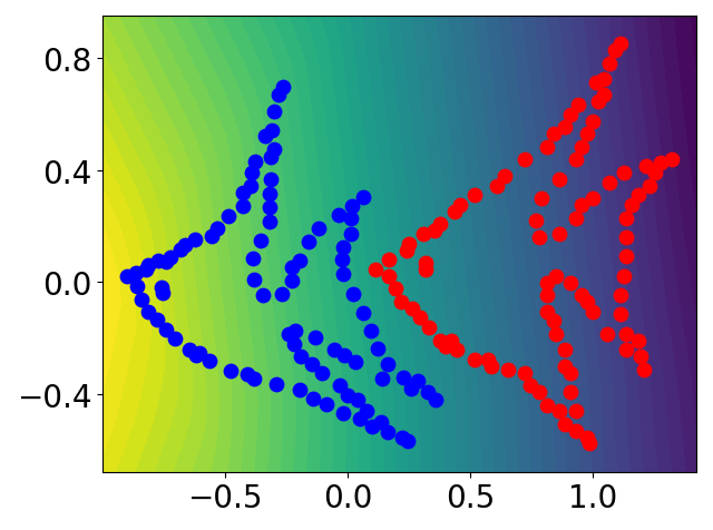
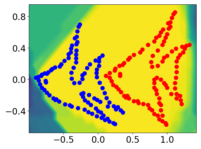
(d) $\mathcal{W}_{1}$, $\mathcal{L}_{M,98}$ or $\mathcal{L}_{D,100}$

Figure 3: Comparison of the primal form and our approximated KR form on discrete distributions $\alpha$ (blue) and $\beta_{\theta}$ (red). The solutions to these two forms are presented in the 1-st and 2-nd row respectively, and the gradients of the potentials are presented in the 3-rd row.

4.3 Algorithm

We now develop a concrete PDM algorithm based on approximated KR forms discussed in Sec. 4.2. We use the following three techniques to facilitate efficient computations. First, we need to ensure that the neural network ${\bm{f}}_{w,h}$ is a valid potential function, i.e., bounded and Lipschitz-1. We ensure the boundedness by defining ${\bm{f}}_{w,h}(x)=\textit{clip}(-|{\bm{f}}_{w}(x)|,-h,0)$, where ${\bm{f}}_{w}$ is a multi-layer perception (MLP) with learnable parameter $w$, and $\textit{clip}(\cdot)$ is the clip function, i.e., we take the negative absolute value of the output of ${\bm{f}}_{w}(x)$, and then clip it to the interval $[-h,0]$. To ensure the Lipschitzness, we add a gradient penalty [43] $\textit{GP}({\bm{f}})=\max_{\hat{x}\in\Omega}\{||\nabla_{\hat{x}}{\bm{f}}(\hat{x})||^{2},1\}$ to the training loss defined below.

Second, to handle continuous or large-scale distributions, we learn ${\bm{f}}_{w,h}$ in a mini-batch manner. Specifically, in each iteration, we sample $\tilde{q}$ and $\tilde{r}$ i.i.d. samples $\{x_{i}\}_{i=1}^{\tilde{q}}$ and $\{y_{i}\}_{i=1}^{\tilde{r}}$ from the normalized distributions $\frac{1}{m_{\alpha}}\alpha$ and $\frac{1}{m_{\beta}}\beta$ respectively, and approximate $\alpha$ and $\beta$ by their empirical distributions: $\tilde{\alpha}=\frac{m_{\alpha}}{\tilde{q}}\sum_{i=1}^{\tilde{q}}\delta_{x_{i}}$ and $\tilde{\beta}=\frac{m_{\beta}}{\tilde{r}}\sum_{i=1}^{\tilde{r}}\delta_{y_{i}}$.

Finally, instead of solving for the optimal ${\bm{f}}^{*}_{w,h}$, we only update ${\bm{f}}_{w,h}$ for a few steps in each iteration to reduce the computation cost. In summary, by combining all three techniques, we optimize

$$\min_{\theta}\max_{\tilde{w}}L(\alpha,\beta_{\theta};\tilde{w})+\mathcal{C}(\theta)$$ (13)

by alternatively updating $\tilde{w}$ and $\theta$ using gradient descent, where

$$L=\frac{m_{\alpha}}{\tilde{q}}\sum_{i=1}^{\tilde{q}} {\bm{f}}_{w,h}(x_{i})-\frac{m_{\beta}}{\tilde{r}}\sum_{j=1}^{\tilde{r}}{\bm{f}}_{w,h}(\mathcal{T}_{\theta}(y_{j}))$$

$$+h(m-m_{\beta})-GP({\bm{f}}_{w,h})$$ (14)

and $\tilde{w}=\{w,h\}$ for $\mathcal{L}_{M,m}$;

$$L=\frac{m_{\alpha}}{\tilde{q}}\sum_{i=1}^{\tilde{q}}{\bm{f}}_{w,h}(x_{i})-\frac{m_{\beta}}{\tilde{r}}\sum_{j=1}^{\tilde{r}} {\bm{f}}_{w,h}(\mathcal{T}_{\theta}(y_{j}))$$

$$-GP({\bm{f}}_{w,h})$$ (15)

and $\tilde{w}=\{w\}$ for $\mathcal{L}_{D,h}$. Note that

$$\nabla_{\theta}L=-\frac{m_{\beta}}{\tilde{r}}\sum_{j=1}^{\tilde{r}}\nabla_{\theta}{\bm{f}}_{w,h}(\mathcal{T}_{\theta}(y_{i})),$$ (16)

and optimizing the min-max problem (13) is generally known as adversarial training [44, 40].

We call our method partial Wasserstein adversarial network (PWAN), and call ${\bm{f}}_{w,h}$ potential network. The detailed algorithm is presented in Alg. 1. For clearness, we refer to PWAN based on $\mathcal{L}_{M,m}$ and $\mathcal{L}_{D,h}$ as mass-type PWAN (m-PWAN) or distance-type PWAN (d-PWAN) respectively. We note that these two types of PWAN are not equivalent despite their close relation. Specifically, for each $(\alpha,\beta_{\theta},m)$, there exists an $h^{*}$ such that the solution to $\mathcal{L}_{D,h^{*}}(\alpha,\beta_{\theta})$ recovers to that of $\mathcal{L}_{M,m}(\alpha,\beta_{\theta})$, but optimizing $\mathcal{L}_{M,m}(\alpha,\beta_{\theta})$ is generally not equivalent to optimizing $\mathcal{L}_{D,h}(\alpha,\beta_{\theta})$ with any fixed $h$, because the corresponding $h^{*}$ depends on $\beta_{\theta}$, which varies during the optimization process.

Algorithm 1 PDM using PWAN

reference distribution $\alpha$, source distribution $\beta$, transform $\mathcal{T}_{\theta}$, network ${\bm{f}}_{w,h}$, network update frequency $u$, training type (“mass” or “distance”), mass threshold $m$ or distance threshold $h$, training step $T$, regularizer $\mathcal{C}_{\theta}$, batch size $\tilde{q}$ and $\tilde{r}$

learned $\theta$

if training type = “mass” then

     $\tilde{w}\leftarrow(w,h)$;  $L\leftarrow$ (4.3)

else if training type = “distance” then

     $\tilde{w}\leftarrow(w)$;  $L\leftarrow$ (4.3)

end if

for $t=1,\ldots,T$ do

     Obtain a mini-batch of $\tilde{q}$ samples $\{x_{i}\}_{i=1}^{\tilde{q}}$ from $\frac{1}{m_{\alpha}}\alpha$.

     Obtain a mini-batch of $\tilde{r}$ samples $\{y_{i}\}_{i=1}^{\tilde{r}}$ from $\frac{1}{m_{\beta}}\beta$.

     for $=1,\ldots,u$ do

         Update $\tilde{w}$ by ascending the gradient $\partial L/\partial\tilde{w}$.

     end for

     Compute the gradient $\partial L/\partial\theta$ according to (16).

     Compute the gradient $\partial\mathcal{C}(\theta)/\partial\theta$.

     Update $\theta$ by descending the gradient $\partial L/\partial\theta+\partial\mathcal{C}/\partial\theta$.

end for

4.4 Connections with WGAN

PWAN includes the well-known WGAN as a special case, because the objective function of WGAN, i.e., $\mathcal{W}_{1}$ is a special case of that of PWAN, i.e., $\mathcal{L}_{M,m}$ and $\mathcal{L}_{D,h}$, and they both approximate the KR forms using neural networks. In other words, when $m_{\alpha}=m_{\beta}=m$ for m-PWAN, or $m_{\alpha}=m_{\beta}$ and $h>diam(\Omega)$ for d-PWAN, they become WGAN.

However, despite its close relations with WGAN, PWAN has a unique property that WGAN does not have: PWAN can automatically omit a fraction of data in the training process. This property can be theoretically explained by observing the learned potential function ${\bm{f}}^{*}$. As for PWAN, $||\nabla{\bm{f}}^{*}||=1$ or $||\nabla{\bm{f}}^{*}||=0$ on the input data (Corollary 2 and 1 in the appendix), i.e., the data points with $0$ gradients will be omitted during training, because they do not contribute to the update of $\theta$ in (16). While for WGAN, $||\nabla{\bm{f}}^{*}||=1$ on the input data (Corollary 1 in [43]), i.e., no data point will be omitted.

Finally, we note that PWAN has an intuitive adversarial explanation as an analogue of WGAN: Let $\alpha$ and $\beta_{\theta}$ be the distribution of real and fake data respectively. During the training process, ${\bm{f}}_{w,h}$ is trying to discriminate $\alpha$ and $\beta_{\theta}$ by assigning each data point a realness score in range $[-h,0]$. The points with the highest score $0$ or the lowest score $-h$ are regarded as the “realest” or “fakest” points respectively. Meanwhile, $\mathcal{T}_{\theta}$ is trying to cheat ${\bm{f}}_{w,h}$ by gradually moving the fake data points to obtain higher scores. However, it does not tend to move the “fakest” points, as their scores cannot be changed easily. The training process ends when $\mathcal{T}_{\theta}$ cannot make further improvements.

5 Applications I: Point Set Registration

This section applies Alg. 1 to point set registration tasks. We present the details of the algorithms in Sec. 5.1, and the numerical results in Sec. 5.2.

5.1 Aligning Point Set Using PWAN

Recall the definition for point set registration in Sec. 4.2: Given $\beta=\sum_{y_{j}\in Y}\delta_{y_{j}}$ and $\alpha=\sum_{x_{i}\in X}\delta_{x_{i}}$, where $Y=\{y_{j}\}_{j=1}^{r}$ and $X=\{x_{i}\}_{i=1}^{q}$ are the source and reference point sets in 3D space. We seek to find an optimal transformation $\mathcal{T}$ that matches $Y$ to $X$ by solving problem (5).

First of all, we define the non-rigid transformation $\mathcal{T}_{\theta}$ parametrized by $\theta=(A,t,V)$ as

$$\mathcal{T}_{\theta}(y_{j})=y_{j}A+t+V_{j},$$ (17)

where $y_{j}\in\mathbb{R}^{1\times 3}$ represents the coordinate of point $y_{j}\in Y$, $A\in\mathbb{R}^{3\times 3}$ is the linear transformation matrix, $t\in\mathbb{R}^{1\times 3}$ is the translation vector, $V\in\mathbb{R}^{r\times 3}$ is the offset vector of all points in $Y$, and $V_{j}$ represents the $j$-th row of $V$.

Then we define the coherence regularizer $\mathcal{C}(\theta)$ similar to [10], i.e., we enforce the offset vector $v_{j}$ to vary smoothly. Formally, let $\mathbf{G}\in\mathbb{R}^{r\times r}$ be a kernel matrix, e.g., the Gaussian kernel $\mathbf{G}_{\rho}(i,j)=e^{-||y_{i}-y_{j}||^{2}/\rho}$, and $\sigma\in\mathbb{R}_{+}$. We define

$$\mathcal{C}(\theta)=\lambda\,Tr(V^{T}(\sigma\mathcal{I}+\mathbf{G}_{\rho})^{-1}V),$$ (18)

where $\lambda\in\mathbb{R}_{+}$ is the strength of constraint, $\mathcal{I}$ is the identity matrix, and $Tr(\cdot)$ is the trace of a matrix.

Since the matrix inversion $(\sigma\mathcal{I}+\mathbf{G}_{\rho})^{-1}$ is computationally expensive, we approximate it via the Nyström method [45], and obtain the gradient

$$\frac{\partial\mathcal{C}(\theta)}{\partial V}\approx 2\lambda\sigma^{-1}(V-\sigma^{-1}\mathbf{Q}(\Lambda^{-1}+\sigma^{-1}\mathbf{Q}^{T}\mathbf{Q})^{-1}\mathbf{Q}^{T}V),$$ (19)

where $\mathbf{G}_{\rho}\approx\mathbf{Q}\Lambda\mathbf{Q}^{T}$, $\mathbf{Q}\in\mathbb{R}^{r\times k}$, $\Lambda\in\mathbb{R}^{k\times k}$ is a diagonal matrix, and $k\ll r$. Note the computational cost of (19) is only $O(r)$ if we regard $k$ as a constant. The detailed derivation is presented in Appx. B.2. Note that $\frac{\partial\mathcal{C}(\theta)}{\partial A}=\frac{\partial\mathcal{C}(\theta)}{\partial t}=0$ since $\mathcal{C}(\theta)$ is not related to $A$ and $t$.

Finally, since it can be shown that $\mathcal{T}_{\theta}$ satisfies the assumption required by Theorem 1 and Theorem 2 (Proposition 9 in the appendix), it is valid to use Alg. 1. We do not adopt the mini-batch setting, i.e., we sample all points in the sets in each iteration: $\tilde{q}=q$ and $\tilde{r}=r$, and set $m_{\alpha}=q$ and $m_{\beta}=r$. For rigid registration tasks, i.e., when $\mathcal{T}_{\theta}$ (17) is required to be a rigid transformation, we simply fix $V=0$ ($\mathcal{C}(\theta)=0$), and define $A$ to be a rotation matrix parametrized by a quaternion.

Due to the approximation error of neural networks, the optimization process often has difficulty converging to the exact local minimum. To address this issue, when the objective function no longer decreases, we replace the objective function by

$$\min_{\theta}\sum_{j=1}^{r}s_{j}||x_{N(j)}-\mathcal{T}_{\theta}(y_{j})||+\mathcal{C}(\theta)$$ (20)

where $x_{N(j)}$ is the closest point to $\mathcal{T}_{\theta}(y_{j})$, and $s_{j}$ is the threshold for point $\mathcal{T}_{\theta}(y_{j})$ defined as

$$s_{j}=\begin{cases}1&if\;||x_{N(j)}-\mathcal{T}_{\theta}(y_{j})||\leq h\\ 0&else\end{cases}$$ (21)

for $\mathcal{L}_{D,h}$, and

$$s_{j}=\begin{cases}1&if\;j\in\textit{Topk}(||\{x_{N(i)}-\mathcal{T}_{\theta}(y_{i})||\}_{i=1}^{r},m)\\ 0&else\end{cases}$$ (22)

for $\mathcal{L}_{M,m}$, where $\textit{Topk}(\cdot,m)$ presents the smallest $m$ elements in $\cdot$. We obtain $\mathcal{T}_{\theta}$ by optimizing (20) until convergence using gradient descent, which generally only takes a few steps. Note that this approach is reasonable because when the point sets are sufficiently well aligned, the closest point pairs are likely to be the corresponding point pairs, thus (20) can be regarded as an approximation of (6).

5.2 Experiments on Point Set Registration

We experimentally evaluate the proposed PWAN on point set registration tasks. We first present a toy example to highlight the robustness of the PW discrepancies in Sec. 5.2.1. Then we compare PWAN against the state-of-the-art methods on synthesized data in Sec. 5.2.2, and discuss its scalability in Sec. 5.2.3. We further evaluate PWAN on real datasets in Sec. 5.2.4. Finally, we present the results of rigid registration in Sec. 5.2.5.

5.2.1 Comparison of Several Discrepancies

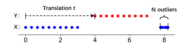
(a) Experimental setting.

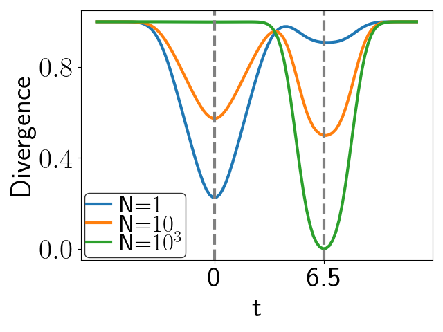
(b) $L_{2}$

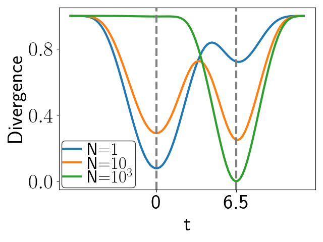
(c) $KL$

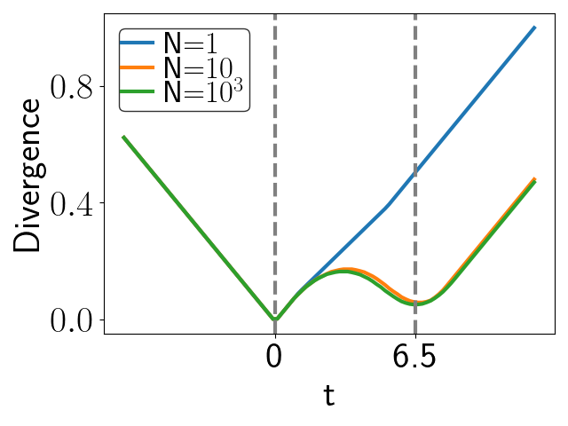
(d) $\mathcal{L}_{M,10}$

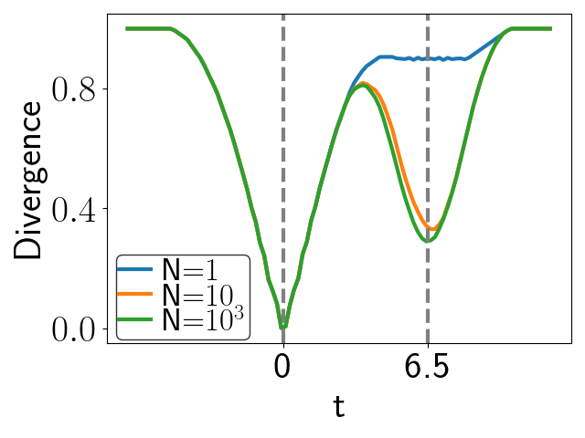
(e) $\mathcal{L}_{D,2}$

Figure 4: Comparison of different discrepancies on a toy point set.

To provide an intuition of the PW divergence $\mathcal{L}_{M,m}$ and $\mathcal{L}_{D,h}$ used in this work, we compare them against two representative robust discrepancies, i.e., KL divergence [30] and $L_{2}$ distance [32], that are commonly used in registration tasks on a toy 1-dimensional example. More discussion can be found in Appx. B.4.

We construct the toy point sets $X$ and $Y$ shown in Fig. 4(a), where we first sample $10$ equi-spaced data points in interval $[0,3]$, then we define $Y$ by translating the data points by $t$, and define $X$ by adding $N$ outliers in a narrow interval $[7.8,8.2]$ to the data points. For $N=\{1,10,10^{3}\}$, we record four discrepancies: KL, $L_{2}$, $\mathcal{L}_{M,10}$ and $\mathcal{L}_{D,2}$ between $X$ and $Y$ as a function of $t$, and present the results from Fig. 4(b) to Fig. 4(e).

By construction, the optimal (perfect) alignment is achieved at $t=0$. However, due to the existence of outliers, there are two alignment modes, i.e., $t=0$ and $t=6.5$ in all settings, where $t=6.5$ represents the biased result. As for KL and $L_{2}$, the local minimum $t=0$ gradually vanishes and they gradually bias toward $t=6.5$ as $N$ increases. In contrast, $\mathcal{L}_{M,10}$ and $\mathcal{L}_{D,2}$ do not suffer from this issue, because the local minimum $t=0$ remains deep, i.e., it is the global minimum, regardless of the value of $N$.

The result suggests that compared to KL and $L_{2}$, $\mathcal{L}_{M,m}$ and $\mathcal{L}_{D,h}$ exhibit stronger robustness against outliers, as the optimal alignment can always be achieved by an optimization process, such as gradient descent, regardless of the ratio of outliers.

5.2.2 Evaluation on Synthesized Data

This section evaluates the performance of PWAN on synthesized data. We use three synthesized datasets shown in Fig. 5: bunny, armadillo and monkey. The bunny and armadillo datasets are from the Stanford Repository [46], and the monkey dataset is from the internet. These shapes consist of $8,171$, $106,289$ and $7,958$ points respectively. We create deformed sets following [47], and evaluate all registration results via mean square error (MSE).

We compare the performance of PWAN with four state-of-the-art methods: CPD [10], GMM-REG [32], BCPD [30] and TPS-RPM [27]. We evaluate all methods in the following two settings:

• Extra noise points: We first sample $500$ random points from the original and the deformed sets as the source and reference sets respectively. Then we add uniformly distributed noise to the reference set, and normalize both sets to mean $0$ and variance $1$. We vary the number of outliers from $100$ to $600$ at an interval of $100$, i.e., the outlier/non-outlier ratio varies from $0.2$ to $1.2$ at an interval of $0.2$.

• Partial overlap: We first sample $1000$ random points from the original and the deformed sets as the source and reference sets respectively. We then intersect each set with a random plane, and retain the points on one side of the plane and discard all points on the other side. We vary the retaining ratio $s$ from $0.7$ to $1.0$ at an interval of $0.05$ for both the source and the reference sets, i.e., the minimal overlap ratio $(2s-1)/s$ varies from $0.57$ to $1$.

We evaluate m-PWAN with $m=500$ in the first setting, while we evaluate m-PWAN with $m=(2s-1)*1000$ and d-PWAN with $h=0.05$ in the second setting. More detailed experiment settings are presented in Appx. B.3. We run all methods $100$ times and report the median and standard deviation of MSE in Fig. 6.

Fig. 6(a) presents the results of the first experiment. The median error of PWAN is generally comparable with TPS-RPM, and is much lower than the other methods. In addition, the standard deviations of the results of PWAN are much lower than that of TPS-RPM. Fig. 6(b) presents the results of the second experiment. Two types of PWANs perform comparably, and they outperform the baseline methods by a large margin in terms of both median and standard deviations when the overlap ratio is low, while all methods perform comparably when the data is fully overlapped. These results suggest the PWAN are more robust against outliers than baseline methods, and can effectively handle partial overlaps. More results are provided in Appx. B.5.

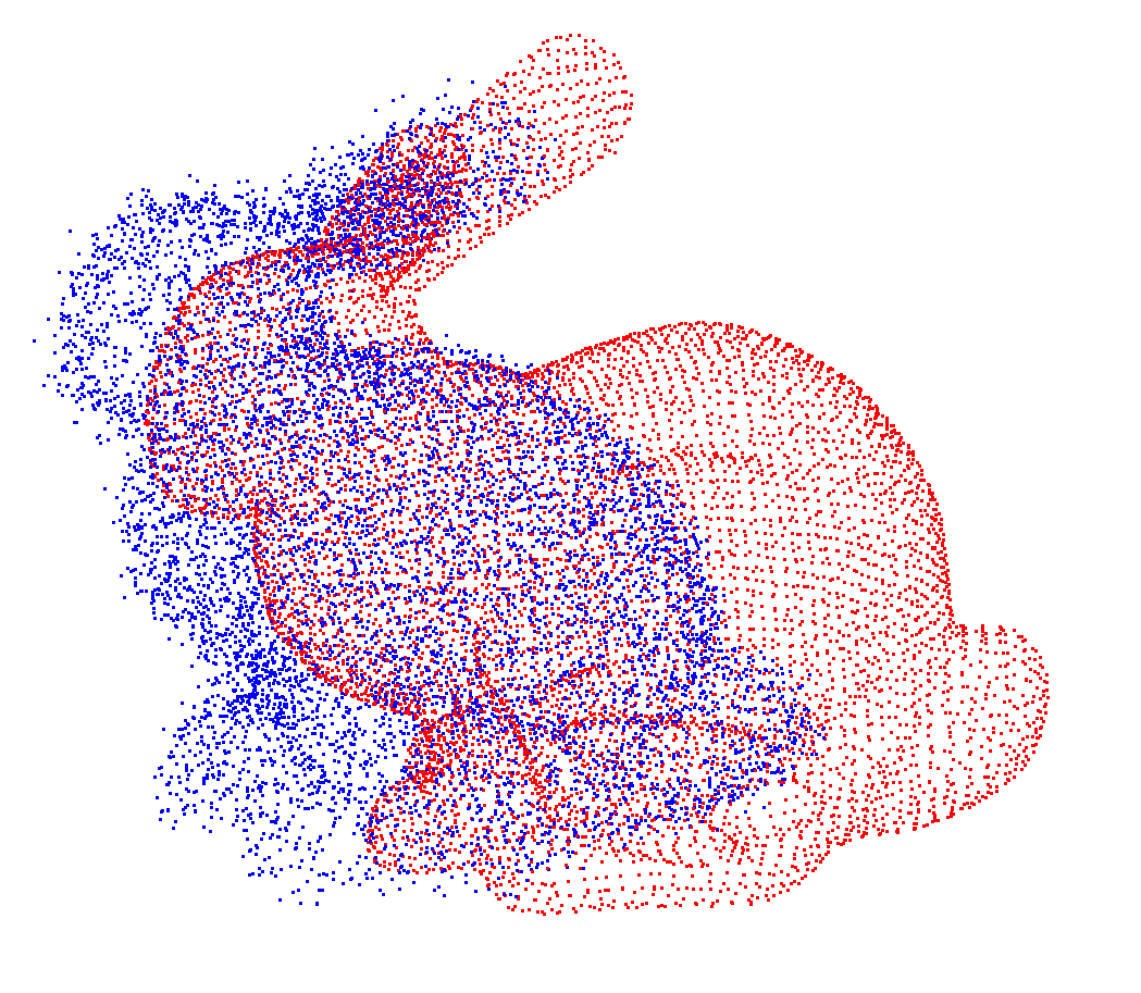
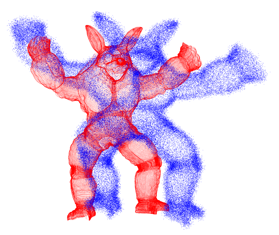
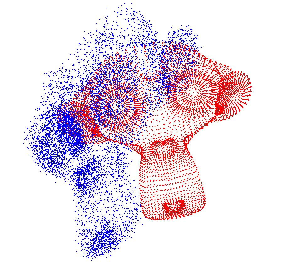
Figure 5: The synthesized datasets used in our experiments.

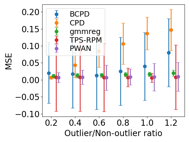
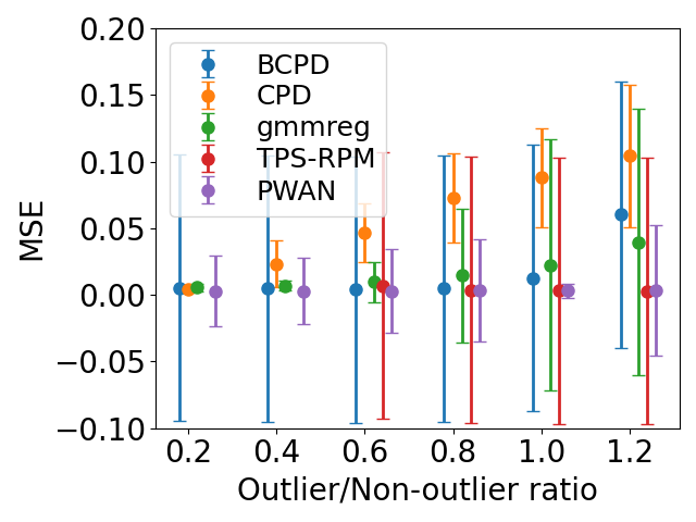
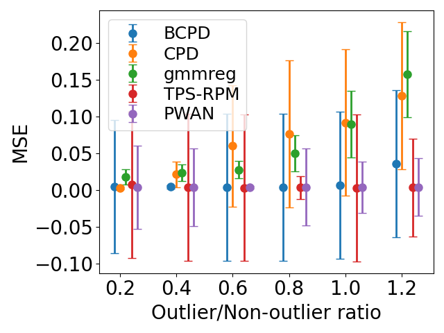
(a) Evaluation of robustness against noise points.

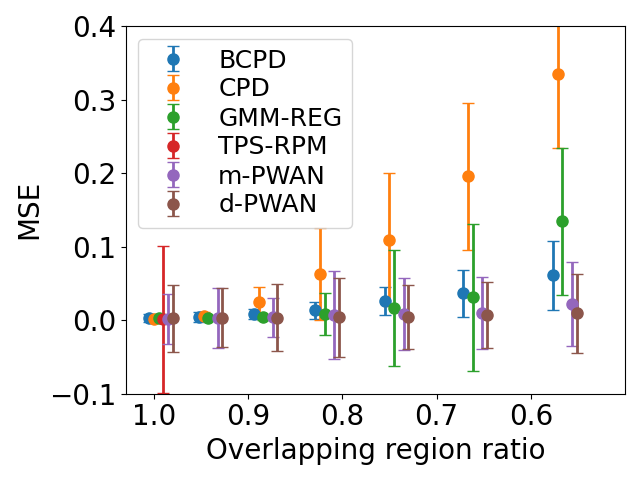
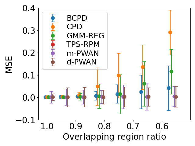
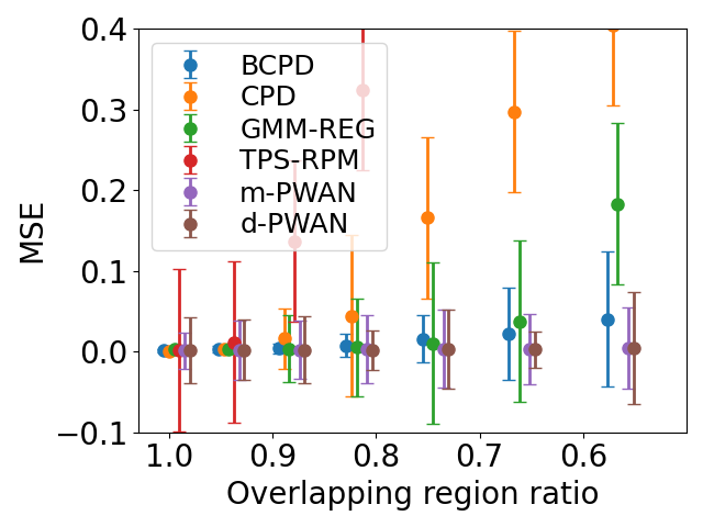
(b) Evaluation of robustness against partial overlap.

Figure 6: Registration accuracy of the bunny (left), monkey (middle) and armadillo (right) datasets. The error bars represent the medians and standard deviations of MSE.

To provide an intuition of the learned potential network of PWAN, we visualize the gradient norm $||\nabla{\bm{f}}_{w,h}||$ on a pair of partially overlapped armadillo point sets at the end of the registration process in Fig. 7. As can be seen, $||\nabla{\bm{f}}_{w,h}||$ is close to $0$ in non-overlapping regions, such as the nose and the left arm, suggesting that the points in these regions are successfully omitted by PWAN.

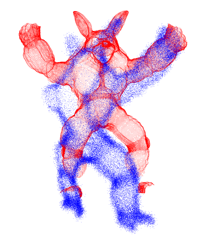
(a) Initial step

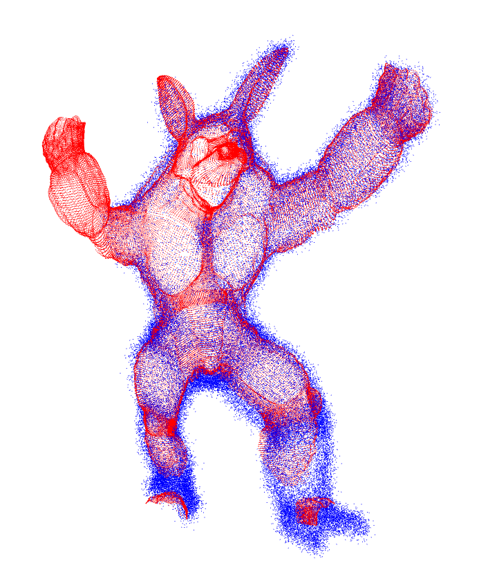
(b) Final step

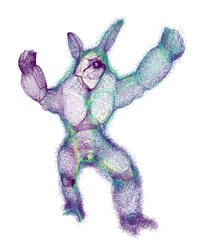
(c) $||\nabla{\bm{f}}_{w,h}||$

Figure 7: Visualization of the learned potential network on a pair of partially overlapped armadillo point sets. $||\nabla{\bm{f}}_{w,h}||$ is lower (darker) in non-overlapping regions, suggesting that the points in those regions are successfully omitted.

5.2.3 Evaluation of the Efficiency

To evaluate the efficiency of PWAN, we first need to investigate the influence of the parameter $u$, i.e., the network update frequency, which is designed to control the tradeoff between efficiency and effectiveness. To this end, we register a pair of bunny datasets consisting of $2000$ points with varying $u$ and report the results on the left panel of Fig. 8. As can be seen, the median and standard deviation of MSE decrease as $u$ increases, and the computation time increases proportionally with $u$, which verifies the effectiveness of $u$.

We then benchmark the computation time of different methods on a computer with two Nvidia GTX TITAN GPUs and an Intel i7 CPU. We fix $u=20$ for PWAN. We sample $q=r$ points from the bunny shape, where $q$ varies from $10^{3}$ to $7\times 10^{5}$. PWAN is run on the GPU while the other methods are run on the CPU. We also implement a multi-GPU version of PWAN where the potential network is updated in parallel. We run each method $10$ times and report the mean of the computation time on the right panel of Fig. 8. As can be seen, BCPD is the fastest method when $q$ is small, and PWAN is comparable with BCPD when $q$ is near $10^{6}$. In addition, the 2-GPU version PWAN is faster than the single GPU version, and it is faster than BCPD when $q$ is larger than $5\times 10^{5}$.

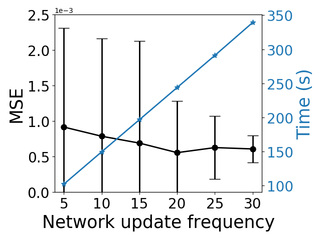
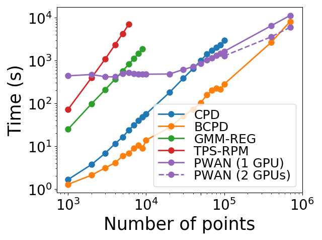
Figure 8: Scalability of PWAN. Left: $u$ controls the tradeoff between efficiency and effectiveness. Right: The speed of PWAN is comparable with that of BCPD when $q$ is near $10^{6}$.

5.2.4 Evaluation on Real Data

To demonstrate the capability of PWAN in handling datasets with non-artificial deformations, we evaluate it on the space-time faces dataset [48] and human shape dataset [49].

The human face dataset [48] consists of a time series of point sets sampled from a real human face. Each face consists of $23,728$ points. We use the faces at time $i$ and $i+20$ as the source and the reference set, where $i=1,...,20$. All point sets in this dataset are completely overlapped. An example of our registration result is presented in Fig. 9. The registration results are quantitatively compared with CPD and BCPD in Tab. VI in the appendix, where PWAN outperforms both baseline methods.

We further evaluate PWAN on the challenging human body dataset [49]. We apply PWAN to both complete and incomplete human shapes. An example of our registration results is shown in Fig. 10, and more details can be found in Appx. B.6. As can be seen, although PWAN is not designed to handle articulated deformations as [50], it can still produce good full-body registration ($1$-st row) and natural partial alignment ($2$-nd row). In addition, it is worth noticing that the partial alignment produces a novel shape that does not exist in the original dataset, which suggests the potential of PWAN in shape editing. Nevertheless, we observe some degree of misalignment near complicated articulated structures, such as fingers. This issue might be addressed by incorporating mesh-level constraints [51] in the future.

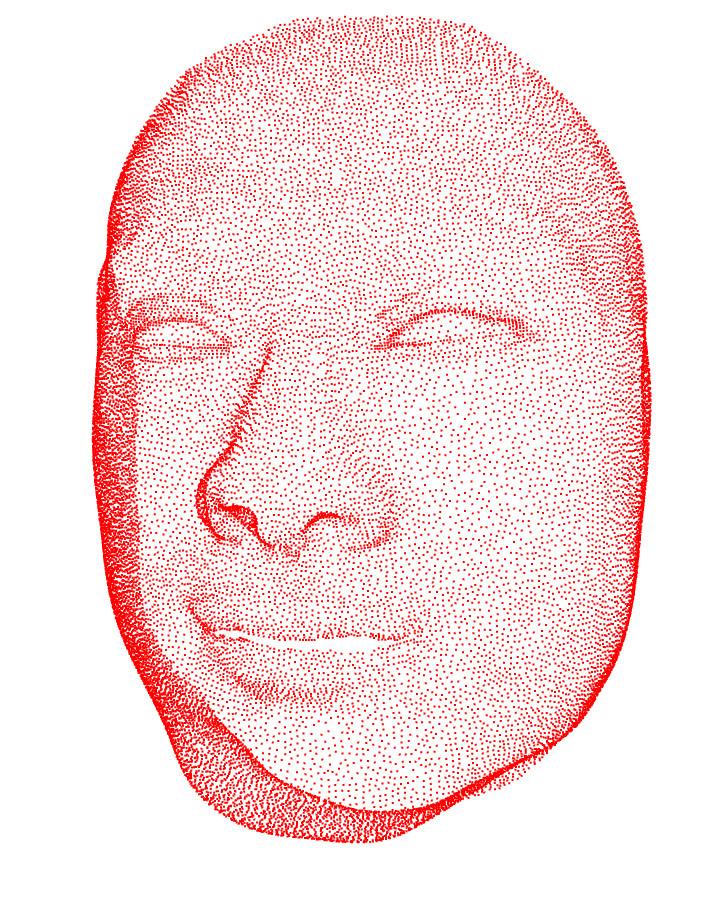
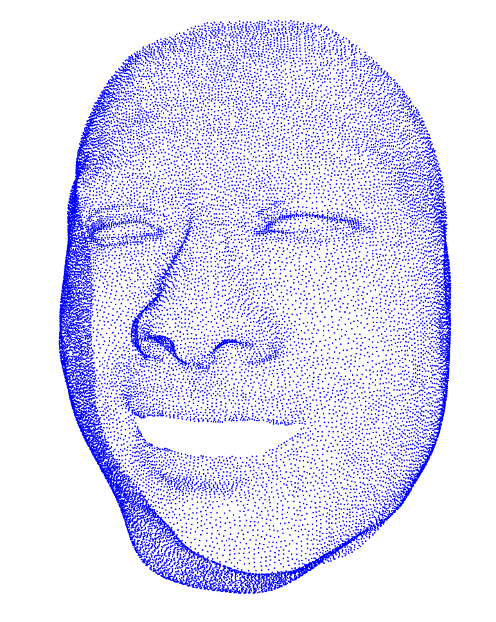
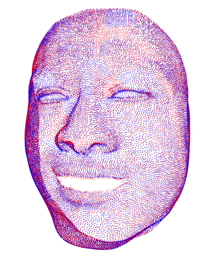
Figure 9: An example of our registration results on the human face dataset. The aligned point sets (right) is obtained by matching the $1$-st frame (left) to the $21$-st frame (middle).

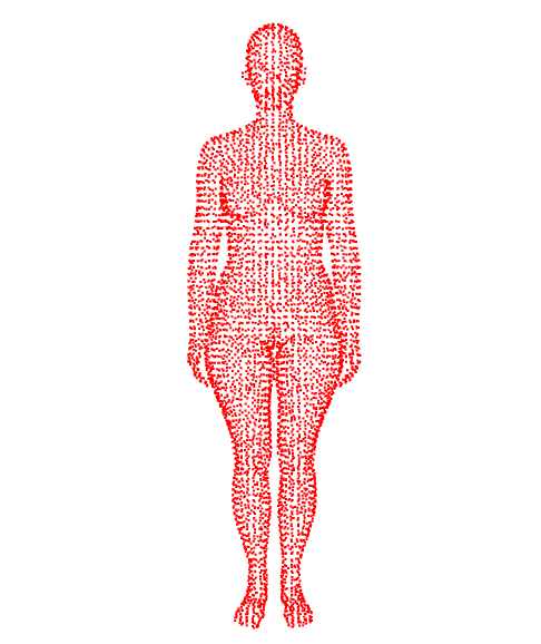
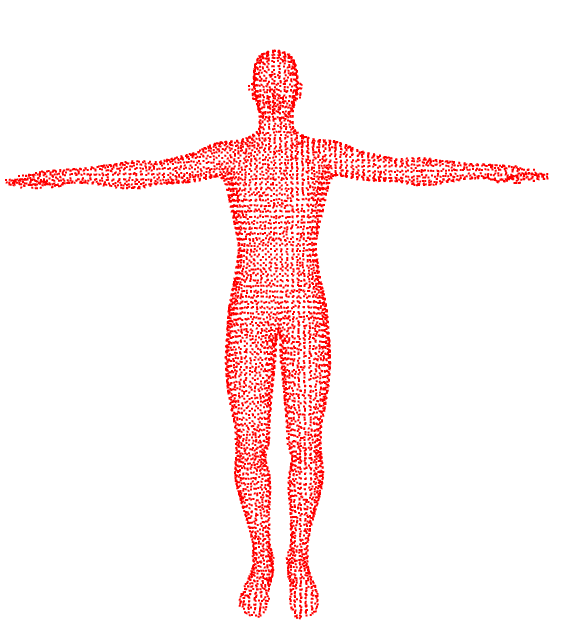
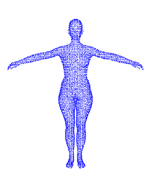
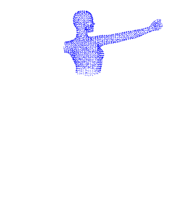
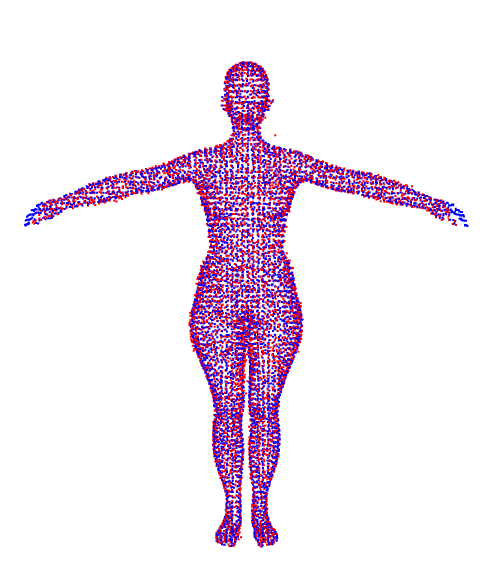
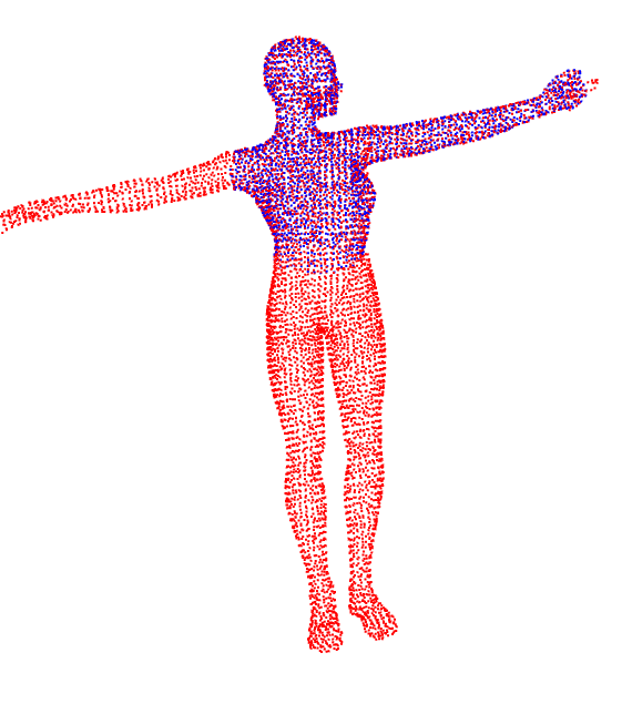
Figure 10: Examples of our registration results on the human body dataset. We present the result of registering complete shapes ($1$-st row) and incomplete shapes ($2$-nd row), where the source point set (left) is aligned to the reference set (middle).

5.2.5 Results of Rigid Registration

PWAN can be naturally applied to rigid registration as a special case of non-rigid registration. We evaluate PWAN on rigid registration using two datasets: ASL [52] and UWA [53]. We construct three registration tasks: outdoor, indoor and object, where the outdoor task consists of two scenes from ASL: mountain and wood-summer, the indoor task consists of two scenes from ASL: stair and apartment, and the object task consists of two scenes from UWA: parasaurolophus and T-rex. For each of the $6$ scenes, we register the $i$-th view to the $(i+1)$-th view, where $i=1,...,10$. We report the rotation error $\frac{180}{\pi}\arccos(\frac{1}{2}(Tr(R\tilde{R}^{T})-1))$, where $R$ and $\tilde{R}$ are the estimated and true rotation matrices respectively. Since UWA dataset does not provide ground true poses, we run the global search algorithm Go-ICP [54] on UWA dataset and use its result as the ground truth.

We pre-process all point sets by normalizing them to be inside the cubic $[-1,1]^{3}$, and down-sampling them using a voxel grid filter with grid size $0.08$. We compare d-PWAN and m-PWAN against BCPD [30], CPD [10], ICP with trimming [55] (m-ICP) and ICP with distance threshold [25, 56] (d-ICP). We set $h=0.05$ for d-PWAN, $m=0.8\min(q,r)$ for m-PWAN, and fix $u=25$.

A quantitative comparison of the registration result is presented in Tab. I, and more details are presented in Appx. B.7. As can be seen, m-PWAN and d-PWAN outperform all baseline methods in all but the object class, where BCPD performs slightly better, and m-PWAN achieves better results than d-PWAN in terms of standard deviation.

TABLE I: Quantitative results of rigid registration. We report the median and standard deviation of rotation errors.

	indoor	outdoor	object
BCPD	0.35 (10.37)	8.08 (8.54)	0.10 (0.26)
CPD	0.79 (28.46)	5.89 (3.95)	0.17 (61.99)
m-ICP	0.54 (22.46)	13.36 (12.37)	1.96 (6.43)
d-ICP	6.62 (18.85)	14.86 (8.20)	21.17 (6.65)
m-PWAN (Ours)	0.26 (14.22)	2.00 (3.62)	0.10 (0.35)
d-PWAN (Ours)	0.26 (22.44)	2.01 (3.63)	0.11 (5.60)

6 Application II: Partial Domain Adaptation

This section applies Alg. 1 to partial domain adaptation tasks. After presenting the details of the method in Sec. 6.1, we show the results of our numerical experiments in Sec. 6.2.

6.1 Partial Domain Adaptation via PWAN

The partial domain adaptation problem is defined as follows. Consider an image classification problem defined on the image space $I$ and the label space $L$. Let $\mathbf{R}$ and $\mathbf{S}$ be the reference and source distributions over $I\times L$, $(\cdot)|_{I}$ be their marginal distributions on $I$, and $L_{(\cdot)}$ be their label sets. For example, $\mathbf{R}_{I}$ is the reference image distribution, and $L_{R}$ consists of all possible labels of $\mathbf{R}$. Given the labelled reference dataset $\mathbf{D}_{R}=\{(x_{i},l_{i})\}_{i=1}^{q}\sim(\mathbf{R})^{q}$ and the unlabeled source dataset $\mathbf{D}_{S}=\{(y_{i})\}_{i=1}^{r}\sim(\mathbf{S}_{I})^{r}$, where $L_{S}$ is assumed to be an unknown subset of $L_{R}$, the goal of partial domain adaptation is to obtain an accurate classifier $\eta$ for $\mathbf{D}_{S}$. Note that following [40, 11], we assume $\eta=\mathcal{D}_{\nu}\circ\mathcal{T}_{\theta}$, where $\mathcal{T}_{\theta}$ is a feature extractor with parameter $\theta$, $\mathcal{D}_{\nu}$ is a label predictor with parameter $\nu$.

The key step in solving adaptation problems is to match $\mathbf{S}_{I}$ to the fraction of $\mathbf{R}_{I}$ belonging to class $L_{S}$ in the feature space, so that the predictor trained on $\mathbf{D}_{R}$ can also be used on $\mathbf{D}_{S}$. We formulate this step as a PDM problem, where the fraction of data in $\mathbf{R}_{I}$ belonging to class $L_{R}\setminus L_{S}$ treated are outliers. Formally, let $\beta_{\theta}=(\mathcal{T}_{\theta})_{\#}\mathbf{S}_{I}$ and $\alpha=(\mathcal{T}_{\widehat{\theta}})_{\#}\mathbf{R}_{I}$ be the feature distributions of $\mathbf{S}_{I}$ and $\mathbf{R}_{I}$ respectively, where $\widehat{\theta}$ denotes a frozen copy of $\theta$ which does not allow back-propagation. We seek to match $\beta_{\theta}$ to $\alpha$ by minimizing $\mathcal{L}_{M,1}(\alpha,\beta_{\theta})$, where we assume $m_{\alpha}\geq m_{\beta}=1$. By combining the PDM formulation with the classifier $\eta$, our complete formulation can be expressed as

$$\min_{\theta,\nu}\sum_{(x_{i},l_{i})\in\mathbf{R}}\mu_{i}\textit{CE}(\eta(x_{i}),l_{i})+\lambda_{1}\mathcal{L}_{M,1}(\alpha,\beta_{\theta})+\lambda_{2}\mathcal{C}(\eta),$$ (23)

where $\mathcal{C}(\eta)$ is the entropy regularizer [57], CE is the cross-entropy loss, $\mu_{i}=\frac{1}{|\mathbf{D_{S}|}}\sum_{y\in\mathbf{D}_{S}}\mathds{1}(\eta(y)=l_{i})$ is the re-weighting coefficient of class $l_{i}$ [58], where the indicator function $\mathds{1}(\cdot)$ equals $1$ if $(\cdot)$ is true, and $0$ otherwise.

To apply PWAN to (23), we first verify that the feed-forward network $\mathcal{T}_{\theta}$ is a valid transformation for PWAN, i.e., it satisfies the assumption required by Theorem 2 (Proposition 10 in the appendix). Then we need to determine the parameter $m_{\alpha}$, which specifies the alignment ratio $1/m_{\alpha}$ of the reference data. If the outlier ratio $r$ of $\alpha$ is known as a prior, we can simply set $m_{\alpha}\approx 1/(1-r)$ to ensure that the correct ratio of data is aligned. However, $r$ is usually unknown in practice, so we first heuristically set $m_{\alpha}$ as $\tilde{m}_{\alpha}=|L_{R}|/|\tilde{L_{S}}|$, where $\tilde{L_{S}}=\{l\in L_{R}|w_{l}>\frac{1}{|L_{R}|}\}$ is the estimated $L_{S}$. This choice of $m_{\alpha}$ is intuitive because it encourages aligning $\tilde{L_{S}}$ classes of data between $\mathbf{D_{R}}$ and $\mathbf{D_{S}}$. Then, to further avoid biasing toward outliers, we gradually increase $m_{\alpha}$ during training. Formally, we set

$$m_{\alpha}=\tilde{m}_{\alpha}\times s^{v}$$ (24)

at training step $v$, where $s>1$ is the annealing factor. An explanation of the effect of $m_{\alpha}$ is presented in Appx. B.8.

Now we can use Alg. 1. We adopt the mini-batch setting and set the batch size $\tilde{q}=\tilde{r}$. For clearness, we provide the explicit formulation of our training goal (23):

$$\min_{\theta,\nu}\max_{w} \sum_{i=1}^{\tilde{q}}\mu_{i}\textit{CE}(\eta(x_{i}),l_{i})+\lambda_{1}\Bigl{(}\frac{m_{\alpha}}{\tilde{q}}\sum_{i=1}^{\tilde{q}}{\bm{f}}_{w}(\mathcal{T}_{\hat{\theta}}(x_{i}))$$

$$- \frac{1}{\tilde{q}}\sum_{i=1}^{\tilde{q}}{\bm{f}}_{w}(\mathcal{T}_{\theta}(y_{i}))-GP({\bm{f}}_{w})\Bigr{)}+\lambda_{2}\mathcal{C}(\eta),$$ (25)

where $\{(x_{i},l_{i})\}_{i=1}^{\tilde{q}}$ is a random batch of $\mathbf{D}_{R}$, $\{(y_{i})\}_{i=1}^{\tilde{q}}$ is a random batch of $\mathbf{D}_{S}$, $m_{\alpha}$ is set according to (24), and ${\bm{f}}_{w}\leq 0$ is the potential network with parameter $w$. The overall network architecture is presented in Fig. 11. By abusing notation, we also call (6.1) PWAN.

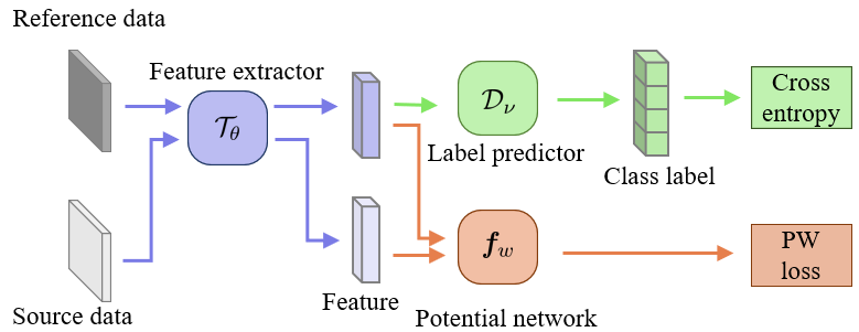
Figure 11: The proposed PWAN for partial domain adaptation.

6.2 Experiments on Partial Domain Adaptation

We experimentally evaluate PWAN on partial domain adaptation tasks. After describing the experimental settings in Sec. 6.2.1, we first present an ablation study in Sec. 6.2.2 to explain the effectiveness of our formulation. Then we compare the performance of PWAN with the state-of-the-art methods in Sec. 6.2.3. We finally discuss parameter selection in Sec. 6.2.4.

6.2.1 Experimental Settings

We construct PWAN as follows: the potential net ${\bm{f}}_{w}$ is a fully connected network with $2$ hidden layers (feature $\rightarrow$ $256$ $\rightarrow$ $256$ $\rightarrow$ $1$); Following [40], the feature extractor $\mathcal{T}_{\theta}$ is defined as a ResNet-50 [59] network pre-trained on ImageNet [60], and the label predictor $\mathcal{D}_{\nu}$ is a fully connected network with $1$ bottleneck layer (feature $\rightarrow$ $256$ $\rightarrow$ label). We update $\{\theta,\nu\}$ using Adam optimizer [61] and update $\{w\}$ using RMSprop optimizer [62], and manually set the learning rate to $1e^{-4}(1+10i)^{-0.75}$ following [40], where $i$ is the training step. We fix $\lambda_{1}=0.05$ and $\lambda_{2}=0.1$ for all experiments. More detailed settings are presented in Appx. B.9.

We consider the following four datasets in our experiments:

• OfficeHome [63]: A dataset consisting of four domains: Artistic (A), Clipart (C), Product (P) and real-world (R). Following [11], we consider all $12$ adaptation tasks between these $4$ domains. We keep all $65$ classes of the reference domain and keep the first $25$ classes (in alphabetic order) of the source domain.

• VisDa17 [64]: A large-scale dataset for synthesis-to-real adaptation, where the reference domain consists of abundant rendered images, and the source domain consists of real images belonging to the same classes. We keep all $12$ classes of the reference domain and keep the first $6$ classes (in alphabetic order) of the source domain.

• ImageNet-Caltech: A challenging large-scale dataset for general-to-specify adaptation. The reference domain is ImageNet [60] ($1000$ classes), and the source domain consists of data from Caltech [65] belonging to the $84$ classes shared by Caltech and ImageNet.

• DomainNet [66]: A recently proposed challenging large-scale dataset. Following [67], we adopt four domains: Clipart (C), Painting (P), Real (R) and Sketch (S). We consider all $12$ adaptation tasks on this dataset. We keep all $126$ classes of the reference domain and keep the first $40$ classes (in alphabetic order) of the source domain.

For clearness, for OfficeHome and DomainNet, we name each task RS-D, where D represents the dataset, R and S represent the reference and source domain respectively. For example, $AC$-OfficeHome represents the task of adapting domain A to domain C on OfficeHome. We omit the dataset name if it is clear from the text.

6.2.2 Ablation Study

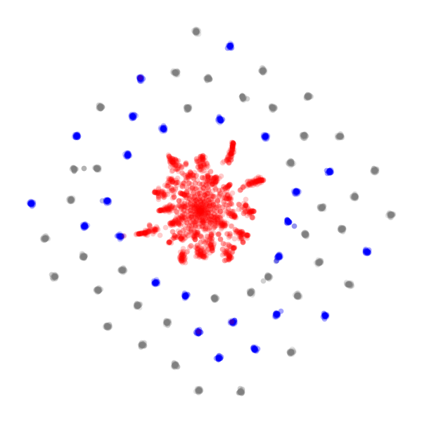
(a) $\lambda_{1}=\lambda_{2}=0$

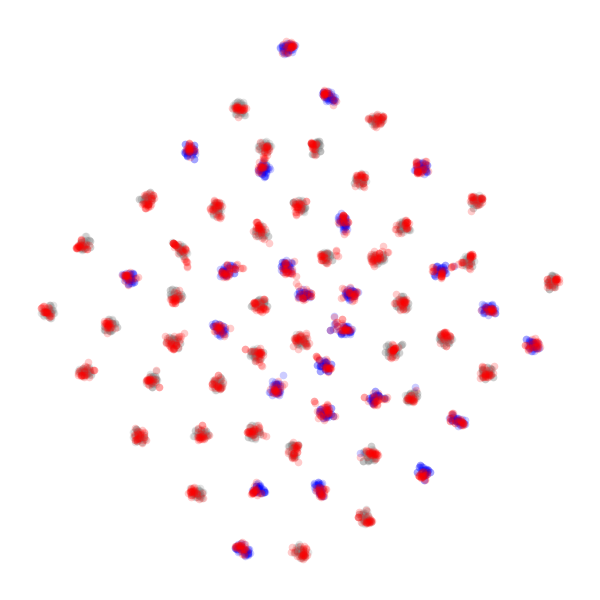
(b) $\lambda_{1}=1,m_{\alpha}=1;\lambda_{2}=0$

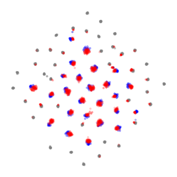
(c) $\lambda_{1}=1,m_{\alpha}=10;\lambda_{2}=0$

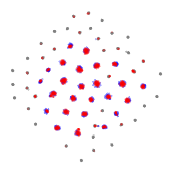
(d) $\lambda_{1}=1,m_{\alpha}=10;\lambda_{2}=0.1$

Figure 12: t-SNE visualization of the learned source and reference features, where blue and grey points represent non-outlier and outlier reference features respectively, and red points represent the source features. PWAN ($\lambda_{1}\neq 0,m_{\alpha}>1$) can align the source features to a fraction of the reference features while avoiding biasing toward outliers.

To explain the effectiveness of formulation (6.1), we conduct an ablation experiment on AR-OfficeHome. We train PWAN with different values of $\{\lambda_{1},m_{\alpha},\lambda_{2}\}$, and visualize the features extracted by $\mathcal{T}_{\theta}$ in Fig. 12 using t-SNE [68]. For clearness, we fix $\mu_{i}=1$ and $s=1$ in this experiment.

When a classifier is trained on the reference data without the aid of PWAN ($\lambda_{1}=\lambda_{2}=0$), the reference and the source feature distributions are well-separated, which suggests that the trained classifier cannot be used for the source data. PWAN ($\lambda_{1}>0$) can alleviate this issue by aligning these two distributions. However, complete alignment ($m_{\alpha}=1$) leads to degraded performance due to serious negative transfer, i.e., most of the source features are biased toward the outlier features. In contrast, by aligning a lower ratio of the reference features, PWAN with larger $m_{\alpha}$ ($m_{\alpha}=10$) can largely avoid the negative transfer effect, i.e., most of the outliers are omitted. In addition, the entropy regularizer ($\lambda_{2}>0$) further improves the alignment as it pushes the source features to their nearest class centers. The results suggest that our formulation (6.1) can indeed align the feature distributions while avoiding negative transfer, which makes the trained classifier suitable for the source data.

TABLE II: Results (accuracy %) of partial domain adaptation on OfficeHome. We additionally report PWAN with extra classification techniques: label smoothing (PWAN+L), complement objective regularizer (PWAN+C), and the combination of these two techniques (PWAN+A).

	AC	AP	AR	CA	CP	CR	PA	PC	PR	RA	RC	RP	Avg
Ref Only	42	67	79.2	56.8	55.9	65.4	59.3	35.5	75.5	68.7	43.4	74.5	60.2
DANN	46.6	45.8	57.5	37.3	32.6	40.5	40.2	39.4	55.4	54.5	44.8	57.6	46.0
PADA	48.9	66.9	81.6	59.1	55.3	65.7	65	41.6	81.1	76	47.6	82	64.2
SAN++	61.25	81.57	88.57	72.82	76.41	81.94	74.47	57.73	87.24	79.71	63.76	86.05	75.96
BAUS	60.6	83.1	88.3	71.7	72.7	83.4	75.4	61.5	86.5	79.2	62.8	86.0	75.9
DPDAN	59.4	—	79.0	—	—	—	—	—	81.7	76.7	58.6	82.1	—
mPOT	64.6	80.6	87.1	76.4	77.6	83.5	77.0	63.7	87.6	81.4	68.5	87.3	77.9
SHOT	62.9 (1.9)	87.0 (0.5)	92.5 (0.1)	75.8 (0.3)	77.0 (1.2)	86.2 (0.6)	77.7 (0.8)	62.8 (0.6)	90.4 (0.5)	81.8 (0.1)	65.5 (0.4)	86.2 (0.1)	78.8 (0.1)
ADV	62.3 (0.4)	82.3 (2.9)	91.5 (0.5)	77.3 (0.9)	76.6 (2.4)	84.9 (2.6)	79.8 (0.8)	63.4 (0.7)	90.1 (0.5)	81.6 (1.1)	65.0 (0.6)	86.6 (0.5)	78.5 (0.4)
PWAN (Ours)	63.5 (3.3)	83.2 (2.7)	89.3 (0.2)	75.8 (1.5)	75.5 (2.5)	83.3 (0.1)	77.0 (2.4)	61.1 (1.5)	86.9 (0.7)	79.9 (0.6)	65.0 (3.8)	86.2 (0.2)	77.2 (1.6)
PWAN+L (Ours)	63.9 (0.1)	84.5 (3.3)	90.3 (0.3)	75.4 (0.9)	75.4 (2.5)	85.2 (1.2)	78.0 (1.6)	63.3 (1.4)	87.5 (0.8)	79.7 (0.7)	66.3 (2.7)	86.5 (0.8)	78.0 (1.4)
PWAN+C (Ours)	63.7 (1.5)	83.6 (2.6)	89.2 (0.4)	76.3 (2.0)	77.1 (3.0)	83.6 (0.1)	77.6 (1.9)	62.2 (0.5)	86.0 (0.4)	79.6 (0.7)	66.2 (2.4)	86.7 (0.3)	77.6 (1.3)
PWAN+A (Ours)	65.2 (0.6)	84.5 (3.0)	89.9 (0.2)	76.7 (0.6)	76.8 (1.9)	84.3 (1.8)	78.7 (3.2)	64.2 (0.9)	87.3 (0.9)	79.9 (1.1)	68.0 (2.3)	86.9 (0.9)	78.5 (1.0)

6.2.3 Results of Partial Domain Adaptation

We compare the performance of PWAN with the state-of-the-art algorithms: DPDAN [69], PADA [12], BAUS [58], SHOT [70], ADV [38], SAN++ [11] and mPOT [23]. We also report the performance of DANN [40], which can be seen as a special case of PWAN for closed-set domain adaptation. We evaluate the performances of all algorithms by the accuracy on the source domain. We run the code of PWAN, ADV and SHOT with $3$ different random seeds and report the mean and standard deviation. The results of other algorithms are adopted from their original papers.

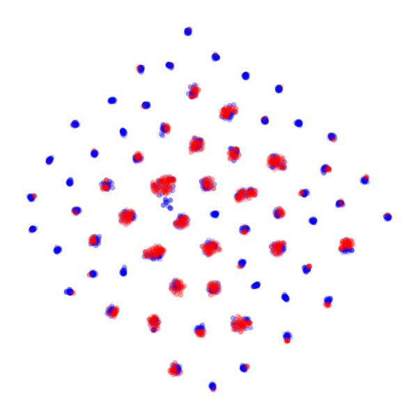
(a) Learned features

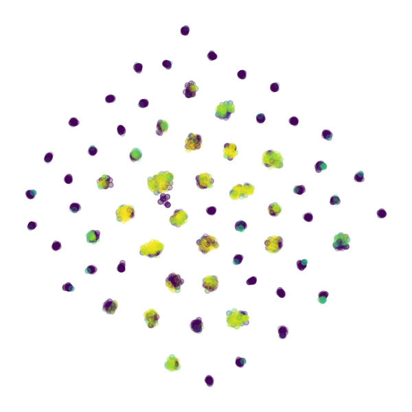
(b) $\|\nabla{\bm{f}}_{w}\|$

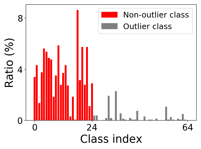
(c) Classification result

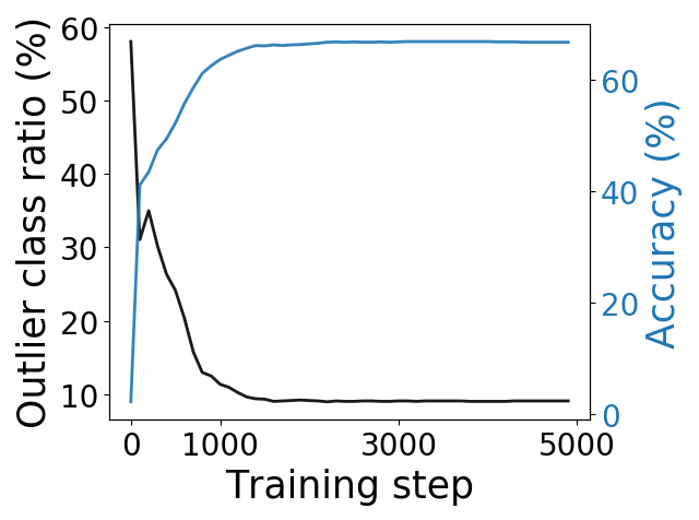
(d) Training process

Figure 13: More detailed results of PWAN on AC-OfficeHome. 13(a) Visualization of the learned features. The red and blue points represent the source and reference features respectively. 13(b) PWAN automatically omits a fraction of reference features (the dark points). 13(c) Most of the source data ($92\%$) is correctly classified into non-outlier classes, i.e., the negative transfer effect is largely avoided. 13(d) During the training process, the test accuracy increases as the ratio of biased source data decreases.

The results on OfficeHome are reported in Tab. II. For a fair comparison, we additionally report the results of PWAN with two advanced techniques developed for discriminative neural networks: complement objective regularizer [71] (PWAN+C) and label smoothing [72] (PWAN+L), and the combination of these two techniques (PWAN+A), as they are also used in ADV, SHOT and BAUS. We observe that PWAN with these techniques (PWAN+A) performs comparably with ADV and SHOT, and they outperform all other methods.

To show the effectiveness of PWAN, we present more training details of PWAN on AC-OfficeHome in Fig. 13. As shown in Fig. 13(a) and Fig. 13(b), the learned source features are matched to a fraction of the reference features, while the other reference features are successfully omitted, i.e., the gradient norm is low on these features. Classification results in Fig. 13(c) show that most of the source data (about 92%) are correctly classified into non-outlier classes, which suggests that the negative transfer effect is largely avoided. In addition, the training process is shown in Fig. 13(d), where we observe that classification accuracy (on the source domain) gradually increases as the biased ratio decreases during the training process. The results show that our training process can effectively narrow the domain gap while avoiding the negative transfer effect.

TABLE III: Results (accuracy %) of partial domain adaptation on ImageNet-Caltech and VisDa17

	ImageNet-Clatech	VisDa17
Source Only	70.6	60.0
DANN	71.4	57.1
PADA	75	66.8
SAN++	83.34	63.0
BAUS	84	69.8
DPDAN	—	65.2
SHOT	83.8 (0.2)	—
ADV	85.4 (0.2)	80.1 (7.9)
PWAN (Ours)	86.0 (0.5)	84.8 (6.1)

TABLE IV: Results (accuracy %) of partial domain adaptation on DomainNet

	CP	CR	CS	PC	PR	PS	RC	RP	RS	SC	SP	SR	Avg
Ref Only	41.2	60.0	42.1	54.5	70.8	48.3	63.1	58.6	50.2	45.4	39.3	49.7	51.9
DANN	27.8	36.6	29.9	31.7	41.9	36.5	47.6	46.8	40.8	25.8	29.5	32.7	35.6
PADA	22.4	32.8	29.9	25.7	56.4	30.4	65.2	63.3	54.1	17.4	23.8	26.9	37.4
BAUS	42.8	54.7	53.7	64.0	76.3	64.6	79.9	74.3	74.0	50.3	42.6	49.6	60.6
ADV	54.1 (3.7)	72.0 (0.4)	55.4 (1.5)	68.8 (0.5)	78.9 (0.2)	75.4 (0.6)	77.4 (0.6)	72.3 (0.5)	70.4 (1.0)	58.4 (0.6)	53.4 (1.6)	65.3 (0.6)	66.8 (0.2)
PWAN (Ours)	54.4 (0.9)	74.1 (1.0)	58.7 (2.5)	65.3 (0.8)	81.4 (0.5)	73.0 (0.6)	78.0 (0.5)	73.4 (0.8)	70.8 (0.7)	51.6 (2.5)	55.1 (0.6)	66.2 (3.3)	66.8 (0.5)

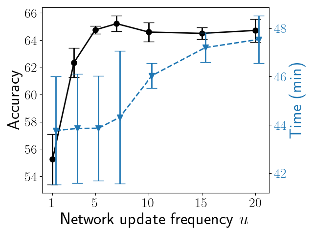
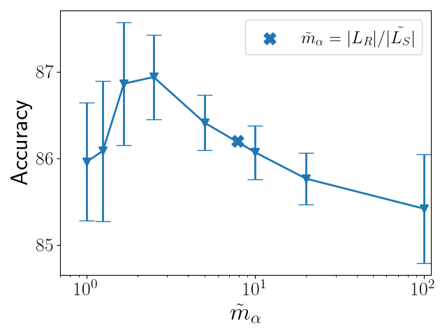
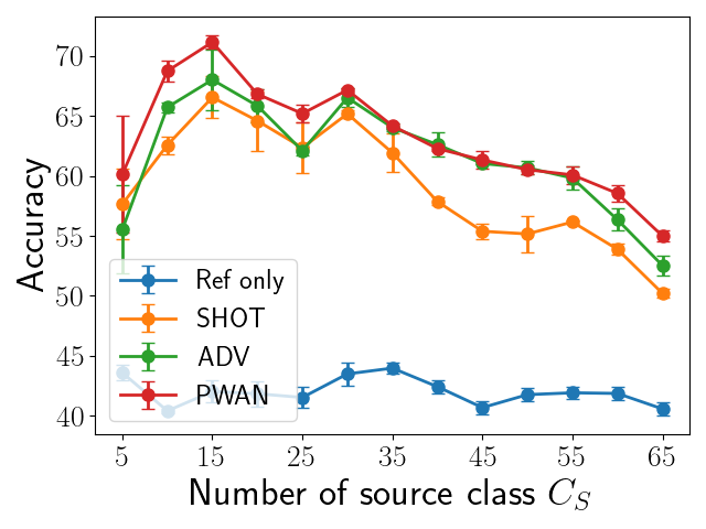
Figure 14: Effect of parameter $m_{\alpha}$ and $u$. Left: The performance and training time of PWAN as functions of $u$. Middle: The performance of PWAN on ImageNet-Caltech with different values of $\tilde{m}_{\alpha}$. Right: Comparison of performance on AC-OfficeHome with different ratios of outlier class.

The results on large-scale datasets VisDa17, ImageNet-Caltech and DomainNet are reported in Tab. III and Tab. IV. On VisDa17, PWAN outperforms all other baseline methods by a large margin. As shown in Fig. 26 in the appendix, PWAN can discriminate all data almost perfectly except for the “knife” and “skateboard” classes which are visually similar. On ImageNet-Caltech, PWAN also outperforms all other baseline methods, which suggests that PWAN can successfully handle datasets dominated by outliers (more than $90\%$ of classes in ImageNet are outlier classes) without complicated sampling techniques [38] or self-training procedures [11]. On DomainNet, PWAN performs comparably with ADV, and outperforms all other methods. More analysis can be found in Appx. B.10.

6.2.4 Effect of Parameters

In this section, we investigate the effects of the two major hyper-parameters involved in PWAN, i.e., $m_{\alpha}$ and $u$, so that they can be intuitively chosen in practical applications without hyper-parameter searching [73].

Parameter $u$ is designed to control the tradeoff between the effectiveness and efficiency of PWAN. To see the practical effects of $u$, we run PWAN on AC-OfficeHome with varying $u$, and report the test accuracy and the corresponding training time in the left panel in Fig. 14. We observe that increasing $u$ leads to more accurate results and longer training time, and the accuracy saturates when $u$ is larger than $10$. Moreover, as $u$ increases from $1$ to $20$, the training time only increases by $10\%$. This result suggests that the cost of training the potential network is small compared to training the classifier, thus relatively large $u$ can be chosen to achieve better performance without causing a heavy computational burden.

Parameter $m_{\alpha}$ (24) is designed to control the alignment ratio, i.e., larger $m_{\alpha}$ indicates that a lower ratio of reference feature will be aligned. To investigate the effects of $m_{\alpha}$, we run PWAN on ImageNet-Caltech with varying $\tilde{m}_{\alpha}$. We update PWAN for $T=48000$ steps, and we fix $s=\exp(10/T)$, i.e., $m_{\alpha}=10\tilde{m}_{\alpha}$ at step $T$. The results are reported in the middle panel of Fig. 14, where we observe that overly large or small $\tilde{m}_{\alpha}$ leads to poor performance, but the variation of performance is not large (about $2\%$) when $\tilde{m}_{\alpha}$ is in the range of $[10^{0},10^{2}]$. This result suggests that the performance of PWAN is stable if a reasonable value of $\tilde{m}_{\alpha}$ is selected.

To further reduce the difficulty of selecting $\tilde{m}_{\alpha}$, we suggested choosing $\tilde{m}_{\alpha}=|L_{R}|/\tilde{|L_{S}|}$ in Sec. 6.1. To see the effectiveness of this selection, we compute the suggested $\tilde{m}_{\alpha}$ for ImageNet-Caltech and mark it in the middle panel of Fig. 14, where we see that although the suggested value is not optimal, it still leads to reasonable performance. We further report the performance of PWAN using the suggested $\tilde{m}_{\alpha}$ on AC-OfficeHome with varying outlier ratio, where we keep the first $C_{S}$ classes (in alphabetic order) in the source domain and vary $C_{S}$ from $5$ to $60$, i.e., the ratio of outlier class varies from $92\%$ to $0\%$. The results are shown in the right panel of Fig. 14, where we observe that the selected $\tilde{m}_{\alpha}$ can indeed handle different outlier ratios, and it enables PWAN to outperform the baseline methods.

7 Conclusion

In this work, we propose PWAN for PDM tasks. To this end, we first derive the KR form and the gradient for the PW divergence. Based on these results, we approximate the PW divergence by a neural network and optimize it via gradient descent. We apply PWAN to point sets registration and partial domain adaptation tasks, and show that PWAN achieves favorable results on both tasks due to its strong robustness against outliers.

There are several issues that need further study. First, when applied to point set registration, the computation time of PWAN is still relatively high. A promising approach to accelerate PWAN is to use a forward generator network as in [74], or to take an optimize-by-learning strategy [75]. Second, it is interesting to explore PWAN in other practical tasks, such as outlier detection [76], and other types of domain adaptation tasks [35, 77, 78].

Appendix A Theoretical results

We first derive the KR duality of $\mathcal{L}_{M,m}$ in Sec. A.1, and then characterize its potential in Sec. A.2. We finally discuss the differentiability in Sec. A.3.

A.1 KR Duality of $\mathcal{L}_{M,m}$

In this subsection, we derive the KR formulation of $\mathcal{L}_{M,m}$. We use the following notations:

• $(\Omega,d)$: a metric $d$ associated with a compact metric space $\Omega$. For example, $\Omega$ is a closed cubic in $\mathbb{R}^{3}$ in point set registration tasks, and $\Omega$ is a closed cubic in $\mathbb{R}^{p}$ in partial domain adaptation tasks, where $p$ is the dimension of features.

• $C(\Omega)$: the set of continuous bounded functions defined on $\Omega$ equipped with the supreme norm.

• $Lip(\Omega)\subseteq C(\Omega)$: the set of 1-Lipschitz function defined on $\Omega$.

• $\mathcal{M}(X)$: the space of Radon measures on space $X$.

• $\pi_{\#}^{1}$: The marginal of $\pi$ on its first variable. Similarly, $\pi_{\#}^{2}$ represents the marginal of $\pi$ on its second variable.

• Given a function $\mathbf{F}$: $X\rightarrow\mathbb{R}\cup+\infty$, the Fenchel conjugate of $\mathbf{F}$ is denoted as $\mathbf{F}^{*}$ and is given by:

  $$\mathbf{F}^{*}(x^{*})=\sup_{x\in X}<x,x^{*}>-\mathbf{F}(x),\quad\forall x^{*}\in X^{*}$$ (26)

  where $X^{*}$ is the dual space of $X$ and $<\cdot>$ is the dual pairing.

Recall the definition of $\mathcal{L}_{M,m}$ and $\mathcal{L}_{D,h}$: for $\alpha,\beta\in\mathcal{M}_{+}(\Omega)$,

$$\mathcal{L}_{M,m}(\alpha,\beta)=\inf_{\pi\in\Gamma_{m}(\alpha,\beta)}\int_{\Omega\times\Omega}c(x,y)d\pi(x,y),$$ (27)

where $c:\Omega\times\Omega\rightarrow\mathbb{R}^{+}$ is a continuous cost function, and $\Gamma_{m}(\alpha,\beta)$ is the set of non-negative measure $\pi$ defined on $\Omega\times\Omega$ satisfying

$$\pi(A\times\Omega)\leq\alpha(A),\quad\pi(\Omega\times A)\leq\beta(A)\quad and\quad\pi(\Omega\times\Omega)\geq m$$

for all measurable set $A\subseteq\Omega$. For ease of notations, we abbreviate $m_{\alpha}=\alpha(\Omega)$, $m_{\beta}=\beta(\Omega)$ and $m(\pi)=\pi(\Omega\times\Omega)$. We also define

$$\mathcal{L}_{D,h}(\alpha,\beta)=\inf_{\pi\in\Gamma_{0}(\alpha,\beta)}\int_{\Omega\times\Omega}c(x,y)d\pi(x,y)-hm(\pi).$$ (28)

where $h>0$ is the Lagrange multiplier.

We first derive the Fenchel-Rockafellar dual of $\mathcal{L}_{M,m}(\alpha,\beta)$.

Proposition 1 (Dual form of $\mathcal{L}_{M,m}$).

(27) can be equivalently expressed as

$$\mathcal{L}_{M,m}(\alpha,\beta)=\sup_{({\bm{f}},{\bm{g}},h)\in\mathbf{R}}\int_{\Omega}{\bm{f}}d\alpha+\int_{\Omega}{\bm{g}}d\beta+mh.$$ (29)

where the feasible set $\mathbf{R}$ is

$$\mathbf{R}=\Bigl{\{}({\bm{f}},{\bm{g}},h)\in C(\Omega)\times C(\Omega)\times\mathbb{R}_{+}|{\bm{f}}\leq 0,\;{\bm{g}}\leq 0,\;c(x,y)-h-{\bm{f}}(x)-{\bm{g}}(y)\geq 0,\forall x,y\in\Omega\Bigr{\}}$$ (30)

In addition, the infimum in (27) is attained.

Proof.

We prove this proposition via Fenchel-Rockafellar duality. We first define space $E$: $C(\Omega)\times C(\Omega)\times\mathbb{R}$, space $F$: $C(\Omega\times\Omega)$, and a linear operator $\mathcal{A}$: $E\rightarrow F$ as

$$\mathcal{A}({\bm{f}},{\bm{g}},h):(x,y)\rightarrow{\bm{f}}(x)+{\bm{g}}(y)+h;\quad\forall{\bm{f}},{\bm{g}}\in C(\Omega),\;\forall h\in\mathbb{R},\;\forall x,y\in\Omega.$$ (31)

Then we introduce a convex function $\mathbf{H}$: $F\rightarrow\mathbb{R}\cup+\infty$ as

$$\mathbf{H}(u)=\begin{cases}0&\;if\;u\geq-c\\ +\infty&\;else\end{cases}$$ (32)

and $\mathbf{L}$: $E\rightarrow\mathbb{R}\cup+\infty$ as

$$\mathbf{L}({\bm{f}},{\bm{g}},h)=\begin{cases}\int{\bm{f}}d\alpha+\int{\bm{g}}d\beta+hm&\;if\;{\bm{f}}\geq 0,\;{\bm{g}}\geq 0,\;h\leq 0\\ +\infty&\;else\end{cases}$$ (33)

We can check when ${\bm{f}}\equiv{\bm{g}}\equiv 1$ and $h=-1$, $\mathbf{H}$ is continuous at $\mathcal{A}({\bm{f}},{\bm{g}},h)$. Thus by Fenchel-Rockafellar duality, we have

$$\inf_{({\bm{f}},{\bm{g}},h)\in E}\mathbf{H}(\mathcal{A}({\bm{f}},{\bm{g}},h))+\mathbf{L}({\bm{f}},{\bm{g}},h)=\sup_{\pi\in\mathcal{M}(\Omega\times\Omega)}-\mathbf{H}^{*}(-\pi)-\mathbf{L}^{*}(\mathcal{A}^{*}\pi)$$ (34)

We first compute $\mathbf{H}^{*}(-\pi)$ and $\mathbf{L}^{*}(\mathcal{A}^{*}\pi)$ on the right-hand side of (34). For arbitrary $\pi\in\mathcal{M}(\Omega\times\Omega)$, we have

$$\mathbf{H}^{*}(-\pi)$$

$$=\sup_{u\in F}\Bigl{\{}\int(-u)d\pi-\mathbf{H}(u)\Bigr{\}}$$

$$=\sup_{u\in F}\Bigl{\{}\int(-u)d\pi|\;u(x,y)\geq-c(x,y),\;\forall(x,y)\in\Omega\times\Omega\Bigr{\}}$$

$$=\sup_{u\in F}\Bigl{\{}\int ud\pi|\;u(x,y)\leq c(x,y),\;\forall(x,y)\in\Omega\times\Omega\Bigr{\}}$$

It is easy to see that if $\pi$ is a non-negative measure, then this supremum is $\int cd\pi$, otherwise it is $+\infty$. Thus

$$\mathbf{H}^{*}(-\pi)=\begin{cases}\int c(x,y)d\pi(x,y)&if\;\pi\in\mathcal{M}_{+}(\Omega\times\Omega)\\ +\infty&else\end{cases}$$ (35)

Similarly, we have

$$\mathbf{L}^{*}(\mathcal{A}^{*}\pi)$$

$$=\sup_{({\bm{f}},{\bm{g}},h)\in E}\Bigl{\{}<({\bm{f}},{\bm{g}},h),A^{*}\pi>-\mathbf{L}({\bm{f}},{\bm{g}},h)\Bigr{\}}$$

$$=\sup_{({\bm{f}},{\bm{g}},h)\in E}\Bigl{\{}<A({\bm{f}},{\bm{g}},h),\pi>-(\int{\bm{f}}d\alpha+\int{\bm{g}}d\beta+hm)|{\bm{f}},{\bm{g}}\geq 0,\;h\leq 0\Bigr{\}}$$

$$=\sup_{({\bm{f}},{\bm{g}},h)\in E}\Bigl{\{}\int{\bm{f}}d(\pi_{\#}^{1}-\alpha)+\int{\bm{g}}d(\pi_{\#}^{2}-\beta)+h(\pi(\Omega\times\Omega)-m)|{\bm{f}},{\bm{g}}\geq 0,\;h\leq 0\Bigr{\}}$$

If $(\alpha-\pi_{\#}^{1})$ and $(\beta-\pi_{\#}^{2})$ are non-negative measures, and $\pi(\Omega\times\Omega)-m\geq 0$, this supremum is $0$, otherwise it is $+\infty$. Thus

$$\mathbf{L}^{*}(\mathcal{A}^{*}\pi)=\begin{cases}0&if(\alpha-\pi_{\#}^{1})\in\mathcal{M}_{+}(\Omega),\;(\beta-\pi_{\#}^{2})\in\mathcal{M}_{+}(\Omega),\;\pi(\Omega\times\Omega)\geq m\\ +\infty&else\end{cases}$$ (36)

In addition, the left-hand side of (34) reads

$$\inf_{({\bm{f}},{\bm{g}},h)\in E}\mathbf{H(\mathcal{A}({\bm{f}},{\bm{g}},h))}+\mathbf{L}({\bm{f}},{\bm{g}},h)$$

$$=\inf_{({\bm{f}},{\bm{g}},h)\in E}\Bigl{\{}\int{\bm{f}}d\alpha+\int{\bm{g}}d\beta+hm|\;{\bm{f}},{\bm{g}}\geq 0,\;h\leq 0,\;{\bm{f}}(x)+{\bm{g}}(y)+h\geq-c(x,y),\forall x,y\in\Omega\Bigr{\}}$$

$$=-\sup_{({\bm{f}},{\bm{g}},h)\in E}\Bigl{\{}\int{\bm{f}}d\alpha+\int{\bm{g}}d\beta+hm|\;{\bm{f}},{\bm{g}}\leq 0,\;h\geq 0,\;{\bm{f}}(x)+{\bm{g}}(y)+h\leq c(x,y),\forall x,y\in\Omega\Bigr{\}}$$

Finally, by inserting these terms into (34), we have

$$\sup_{\begin{subarray}{c}({\bm{f}},{\bm{g}},h)\in E\\ {\bm{f}},{\bm{g}}\leq 0,h\geq 0\\ {\bm{f}}(x)+{\bm{g}}(y)+h\leq c(x,y)\forall x,y\in\Omega\end{subarray}}\int{\bm{f}}d\alpha+\int{\bm{g}}d\beta+hm=\inf_{\begin{subarray}{c}\pi\in\mathcal{M}_{+}(\Omega\times\Omega)\\ (\alpha-\pi_{\#}^{1})\in\mathcal{M}_{+}(\Omega),(\beta-\pi_{\#}^{2})\in\mathcal{M}_{+}(\Omega)\\ \pi(\Omega\times\Omega)\geq m\end{subarray}}\int c(x,y)d\pi(x,y),$$

which proves (29).

In addition, we can also check right-hand side of (34) is finite, since we can always construct independent coupling $\widetilde{\pi}=\frac{m}{\alpha(\Omega)\beta(\Omega)}\alpha\otimes\beta$, such that $\widetilde{\pi}\in\mathcal{M}_{+}(\Omega\times\Omega)$, $\widetilde{\pi}_{\#}^{1}=\frac{m}{\alpha(\Omega)}\alpha\leq\alpha$, $\widetilde{\pi}_{\#}^{2}=\frac{m}{\beta(\Omega)}\beta\leq\beta$ and $\widetilde{\pi}(\Omega\times\Omega)=m$. Thus the Fenchel-Rockafellar duality suggests the infimum is attained. ∎

Similarly, we can derive the Fenchel-Rockafellar dual form of $\mathcal{L}_{D,h}$.

Proposition 2 (Dual form of $\mathcal{L}_{D,h}$).

(28) can be equivalently expressed as

$$\mathcal{L}_{D,h}(\alpha,\beta)=\sup_{({\bm{f}},{\bm{g}})\in\mathbf{R}(h)}\int_{\Omega}{\bm{f}}d\alpha+\int_{\Omega}{\bm{g}}d\beta.$$ (37)

where the feasible set is

$$\mathbf{R}(h)=\Bigl{\{}({\bm{f}},{\bm{g}})\in C(\Omega)\times C(\Omega)|{\bm{f}}\leq 0,\;{\bm{g}}\leq 0,\;c(x,y)-h-{\bm{f}}(x)-{\bm{g}}(y)\geq 0,\forall x,y\in\Omega\Bigr{\}}$$ (38)

In addition, the infimum in (28) is attained.

By comparing Proposition 2 with Proposition 1, we can see that $\mathcal{L}_{D,h}$ and $\mathcal{L}_{M,m}$ are related by

$$\mathcal{L}_{M,m} =\sup_{({\bm{f}},{\bm{g}},h)\in\mathbf{R}}\int_{\Omega}{\bm{f}}d\alpha+\int_{\Omega}{\bm{g}}d\beta+mh$$

$$=\sup_{h\in\mathbb{R}_{+}}\mathcal{L}_{D,h}+mh.$$ (39)

Therefore, when the cost function $c$ is the distance ${\bm{d}}$, we obtain the KR form of $\mathcal{L}_{M,m}$ by inserting (4) into (A.1).

Proposition 3 (KR form of $\mathcal{L}_{M,m}$).

When $c(x,y)={\bm{d}}(x,y)$, (27) can be reformulated as

$$\mathcal{L}_{M,m}(\alpha,\beta)=\sup_{\begin{subarray}{c}{\bm{f}}\in Lip(\Omega),h\in\mathbf{R}_{+}\\ -h\leq{\bm{f}}\leq 0\end{subarray}}\int_{\Omega}{\bm{f}}d\alpha-\int_{\Omega}{\bm{f}}d\beta+h(m-m_{\beta})$$ (40)

or equivalently as

$$\mathcal{L}_{M,m}(\alpha,\beta)=\sup_{{\bm{f}}\in Lip(\Omega),{\bm{f}}\leq 0}\int_{\Omega}{\bm{f}}d\alpha-\int_{\Omega}{\bm{f}}d\beta-\inf({\bm{f}})(m-m_{\beta}).$$ (41)

Proof.

For equation (41), note that given an ${\bm{f}}\in C(\Omega)$, the optimal $h$ is simply $-\inf({\bm{f}})<+\infty$ (${\bm{f}}$ is continuous and $\Omega$ is compact). So we can replace $h$ by $-\inf({\bm{f}})$ in (40) to obtain (41). ∎

For simplicity, we define some functionals associated with $\mathcal{L}_{M,m}$ and $\mathcal{L}_{D,h}$.

Definition 1 ($\mathbf{L}_{M,m}$ and $\overline{\mathbf{L}_{M,m}}$).

Define

$$\mathbf{L}_{M,m}^{\alpha,\beta}({\bm{f}},h)=\begin{cases}\int_{\Omega}{\bm{f}}d(\alpha-\beta)+h(m-m_{\beta})&h\in\mathbb{R}_{+}\;,\;{\bm{f}}\in Lip(\Omega)\;,\;-h\leq{\bm{f}}\leq 0\\ -\infty&else,\end{cases}$$

and

$$\overline{\mathbf{L}_{M,m}^{\alpha,\beta}}({\bm{f}})=\begin{cases}\int_{\Omega}{\bm{f}}d(\alpha-\beta)-\inf({\bm{f}})(m-m_{\beta})&{\bm{f}}\in Lip(\Omega)\;,\;{\bm{f}}\leq 0\\ -\infty&else.\end{cases}$$

Definition 2 ($\mathbf{L}_{D,h}$).

$$\mathbf{L}_{D,h}^{\alpha,\beta}({\bm{f}})=\begin{cases}\int_{\Omega}{\bm{f}}d\alpha-\int_{\Omega}{\bm{f}}d\beta-hm_{\beta}&{\bm{f}}\in Lip(\Omega)\;,\;-h\leq{\bm{f}}\leq 0,\\ -\infty&else.\end{cases}$$

We also define the functional associated with Wasserstein-1 metric $\mathcal{W}_{1}$:

Definition 3 ($\mathbf{W}_{1}$).

$$\mathbf{W}^{\alpha,\beta}({\bm{f}})=\begin{cases}\int_{\Omega}{\bm{f}}d\alpha-\int_{\Omega}{\bm{f}}d\beta&{\bm{f}}\in Lip(\Omega),\;m_{\alpha}=m_{\beta}\\ -\infty&else,\end{cases}$$ (42)

With these definitions, we can write

$$\mathcal{L}_{D,h}(\alpha,\beta)=\sup_{{\bm{f}}\in C(\Omega)}\mathbf{L}_{D,h}^{\alpha,\beta}({\bm{f}}),$$

$$\mathcal{L}_{M,m}(\alpha,\beta)=\sup_{{\bm{f}}\in C(\Omega),h\in\mathbb{R}}\mathbf{L}_{M,m}^{\alpha,\beta}({\bm{f}},h)\;\;and\;\;\mathcal{L}_{M,m}(\alpha,\beta)=\sup_{{\bm{f}}\in C(\Omega)}\overline{\mathbf{L}_{M,m}^{\alpha,\beta}}({\bm{f}}),\;$$

and

$$\mathcal{W}_{1}(\alpha,\beta)=\sup_{{\bm{f}}\in C(\Omega)}\mathbf{W}^{\alpha,\beta}({\bm{f}}).$$

For simplicity, we omit the notation of $\alpha$ and $\beta$ where they are clear from the text.

A.2 Properties of KR Potentials

Before we can discuss the property of the KR potential, i.e., the maximizer of $\mathbf{L}_{M,m}$ and $\mathbf{L}_{D,h}$, we first need to show that the potentials exist. As for $\mathbf{L}_{D,h}$, the existence of potentials is already known in [18]:

Proposition 4 ([18]).

For $\alpha,\beta\in\mathcal{M}_{+}(\Omega)$ and $h>0$, there exists an ${\bm{f}}^{*}\in C(\Omega)$ such that $\mathcal{L}_{D,h}(\alpha,\beta)=\mathbf{L}_{D,h}^{\alpha,\beta}({\bm{f}}^{*})$.

As for $\mathbf{L}_{M,m}$, we can also prove the existence of the maximizer similarly:

Proposition 5.

For $\alpha,\beta\in\mathcal{M}_{+}(\Omega)$ and $m>0$, there exist ${\bm{f}}^{*}\in C(\Omega)$ and $h\in\mathbb{R}$ such that $\mathcal{L}_{M,m}(\alpha,\beta)=\mathbf{L}_{M,m}^{\alpha,\beta}({\bm{f}}^{*},h)$.

To prove this proposition, we need the following lemma.

Lemma 1 (Continuity).

$\mathbf{L}_{M,m}^{\alpha,\beta}$ is continuous on $C(\Omega)\times\mathbb{R}$.

Proof.

Let $({\bm{f}}_{n},h_{n})\rightarrow({\bm{f}},h)$ in $C(\Omega)\times\mathbb{R}$. Assume $\mathbf{L}_{M,m}^{\alpha,\beta}({\bm{f}}_{n},h_{n})>-\infty$ when $n$ is sufficiently large. We first check $\mathbf{L}_{M,m}^{\alpha,\beta}({\bm{f}},h)>-\infty$ as follows. For arbitrary $\epsilon>0$, there exists $N>0$ such that for $n>N$, $h_{n}<h+\epsilon$, thus ${\bm{f}}_{n}>-h_{n}>-h-\epsilon$. By taking $n\rightarrow\infty$, we see for arbitrary $\epsilon>0$, ${\bm{f}}>-h-\epsilon$, which suggests ${\bm{f}}\geq-h$. In addition, it is easy to see ${\bm{f}}\leq 0$ and $h\geq 0$. It is also easy to see $Lip({\bm{f}})\leq 1$ due to the closeness of $Lip(\Omega)$. Thus according to definition 1, we claim $\mathbf{L}_{M,m}^{\alpha,\beta}({\bm{f}},h)>-\infty$. Furthermore, since $-h-\epsilon<{\bm{f}}_{n}<0$, and ${\bm{f}}_{n}\rightarrow{\bm{f}}$, by dominated convergence theorem, we have

$$\lim_{n\rightarrow\infty}\int_{\Omega}{\bm{f}}_{n}d\alpha=\int_{\Omega}\lim_{n\rightarrow\infty}{\bm{f}}_{n}d\alpha=\int_{\Omega}{\bm{f}}d\alpha,$$ (43)

$$and \lim_{n\rightarrow\infty}\int_{\Omega}{\bm{f}}_{n}d\beta=\int_{\Omega}\lim_{n\rightarrow\infty}{\bm{f}}_{n}d\beta=\int_{\Omega}{\bm{f}}d\beta.$$ (44)

Note we also have $h_{n}(m-m_{\beta})\rightarrow h(m-m_{\beta})$. We conclude the proof by combining these three terms and obtaining $\mathbf{L}_{M,m}^{\alpha,\beta}({\bm{f}}_{n},h_{n})\rightarrow\mathbf{L}_{M,m}^{\alpha,\beta}({\bm{f}},h)$. ∎

Proof of Proposition 5.

If we can find a maximizing sequence $({\bm{f}}_{n},h_{n})$ that converges to $({\bm{f}},h)\in C(\Omega)\times\mathbb{R}$, then Lemma 1 suggests that $\mathcal{L}_{M,m}(\alpha,\beta)=\sup_{{\bm{f}},h}\mathbf{L}_{M,m}^{\alpha,\beta}({\bm{f}},h)=\lim_{n\rightarrow\infty}\mathbf{L}_{M,m}^{\alpha,\beta}({\bm{f}}_{n},h_{n})=\mathbf{L}_{M,m}^{\alpha,\beta}({\bm{f}},h)$, which proves this proposition. Therefore, we only need to show that it is always possible to construct such a maximizing sequence.

Let $({\bm{f}}_{n},h_{n})$ be a maximizing sequence. We abbreviate $\max({\bm{f}}_{n})=\max_{x\in\Omega}({\bm{f}}_{n}(x))$ and $\min({\bm{f}}_{n})=\min_{x\in\Omega}({\bm{f}}_{n}(x))$. We first assume ${\bm{f}}_{n}$ does not have any bounded subsequence, then there exists $N>0$, such that for all $n>N$, $\min({\bm{f}}_{n})<-diam(\Omega)$ (otherwise we can simply collect a subsequence of ${\bm{f}}_{n}$ bounded by $diam(\Omega)$). We can therefore construct $\widetilde{{\bm{f}}_{n}}={\bm{f}}_{n}-(\min({\bm{f}}_{n})+diam(\Omega))$ and $\widetilde{h_{n}}=h_{n}+(\min({\bm{f}}_{n})+diam(\Omega))$. Note that $\max(\widetilde{{\bm{f}}_{n}})\leq\min(\widetilde{{\bm{f}}_{n}})+diam(\Omega)=-diam(\Omega)+diam(\Omega)=0$, $\widetilde{{\bm{f}}_{n}}+\widetilde{h_{n}}={\bm{f}}_{n}+h_{n}\geq 0$, and $\widetilde{{\bm{f}}_{n}}\in Lip(\Omega)$, so $\mathbf{L}_{M,m}^{\alpha,\beta}(\widetilde{{\bm{f}}_{n}},\widetilde{h_{n}})>-\infty$, and

$$\mathbf{L}_{M,m}^{\alpha,\beta}(\widetilde{{\bm{f}}_{n}},\widetilde{h_{n}}) =\int_{\Omega}\widetilde{{\bm{f}}_{n}}d(\alpha-\beta)+\widetilde{h_{n}}(m-m_{\beta})$$

$$=\int_{\Omega}{\bm{f}}_{n}d(\alpha-\beta)+h_{n}(m-m_{\beta})+(\min({\bm{f}}_{n})-diam(\Omega))(m-m_{\alpha})$$

$$\geq\mathbf{L}_{M,m}^{\alpha,\beta}({\bm{f}}_{n},h_{n}),$$

which suggests that $(\widetilde{{\bm{f}}_{n}},\widetilde{h_{n}})$ is a better maximizing sequence than $({\bm{f}}_{n},h_{n})$. Note that $\widetilde{{\bm{f}}_{n}}$ is uniformly bounded by $diam(\Omega)$ because $0\geq\widetilde{{\bm{f}}_{n}}\geq\min(\widetilde{{\bm{f}}_{n}})=-diam(\Omega)$. As a result, we can always assume $\widetilde{h_{n}}$ is also bounded by $diam(\Omega)$. Because otherwise we can construct $\overline{h_{n}}=-\min(\widetilde{{\bm{f}}_{n}})\leq diam(\Omega)$, and it is easy to show $(\widetilde{{\bm{f}}_{n}},\overline{h_{n}})$ is a better maximizing sequence than $(\widetilde{{\bm{f}}_{n}},\widetilde{h_{n}})$. In summary, we can always find a maximizing sequence $({\bm{f}}_{n},h_{n})$, such that both ${\bm{f}}_{n}$ and $h_{n}$ are bounded by $diam(\Omega)$.

Finally, since ${\bm{f}}_{n}$ is uniformly bounded and equicontinuous, ${\bm{f}}_{n}$ converges uniformly (up to a subsequence) to a continuous function ${\bm{f}}$. In addition, $h_{n}$ has a convergent subsequence since it is bounded. Therefore, we can always find a maximizing sequence $({\bm{f}}_{n},h_{n})$ that converges to some $({\bm{f}},h)\in C(\Omega)\times\mathbb{R}$, which finishes the proof. ∎

Remark The proof of Proposition 5 is an analogue of Proposition 2.11 in [18]. The difference is that in Proposition 5, besides ${\bm{f}}$, we additionally need to handle another variable $h$ acting as the lower bound of ${\bm{f}}$.

Now we proceed to the main result in this subsection, which states that the potential is $0$ or $-h$ on the omitted mass, thus it has $0$ gradient on this mass. This qualitative description reveals an interesting connection between our algorithm and WGAN [1].

First, we note that, the potential of $\mathcal{W}_{1}$ can be characterized as follows.

Lemma 2 (Potential of $\mathcal{W}_{1}$ [43]).

Let ${\bm{f}}^{*}$ be a maximizer of $\mathbf{W}_{1}^{\alpha,\beta}$. If ${\bm{f}}^{*}$ is differentiable, and there exists a primal solution $\pi$ satisfying $\pi(x=y)=0$, then ${\bm{f}}^{*}$ has gradient norm $1$ $(\alpha+\beta)$-almost surely.

Then we characterize the flatness of the potential of $\mathcal{L}_{D,h}$ in the following two lemmas.

Lemma 3.

Let $\pi$ be the solution to the primal form of $\mathcal{L}_{D,h}(\alpha,\beta)$. Assume $\alpha^{\prime},\beta^{\prime}\in\mathcal{M}(\Omega)$ satisfy

$$\pi_{\#}^{1}\leq\alpha^{\prime}\leq\alpha\quad and\quad\pi_{\#}^{2}\leq\beta^{\prime}\leq\beta.$$ (45)

(1) $\pi$ is also the solution to the primal form of $\mathcal{L}_{D,h}(\alpha^{\prime},\beta^{\prime})$ and $\mathcal{W}_{1}(\pi_{\#}^{1},\pi_{\#}^{2})$, thus

$$\mathcal{L}_{D,h}(\alpha,\beta)=\mathcal{L}_{D,h}(\alpha^{\prime},\beta^{\prime})=\mathcal{W}_{1}(\pi_{\#}^{1},\pi_{\#}^{2})-hm(\pi)$$ (46)

(2) Let ${\bm{f}}^{*}$ be a maximizer of $\mathbf{L}_{D,h}^{\alpha,\beta}$. Then ${\bm{f}}^{*}$ is also a maximizer of $\mathbf{L}_{D,h}^{\alpha^{\prime},\beta^{\prime}}$ and $\mathbf{W}_{1}^{\pi_{\#}^{1},\pi_{\#}^{2}}$.

Proof.

(1) First, it is easy to verify that $\pi$ is indeed an admissible solution to the primal form of $\mathcal{L}_{D,h}(\alpha^{\prime},\beta^{\prime})$. Then, notice that all the admissible solutions to the primal form of $\mathcal{L}_{D,h}(\alpha^{\prime},\beta^{\prime})$ are also admissible solutions to the primal form of $\mathcal{L}_{D,h}(\alpha,\beta)$. Finally, we can conclude by contradiction: If there exists a better solution than $\pi$ for $\mathcal{L}_{D,h}(\alpha^{\prime},\beta^{\prime})$, then it is also better than $\pi$ for $\mathcal{L}_{D,h}(\alpha,\beta)$, which contradicts the optimality of $\pi$. Similarly, we can prove that $\pi$ is also the solution to $\mathcal{W}_{1}(\pi_{\#}^{1},\pi_{\#}^{2})$.

(2) Note we have

$$\mathbf{L}_{D,h}^{\alpha^{\prime},\beta^{\prime}}({\bm{f}}^{*})=\int_{\Omega}{\bm{f}}^{*}d\alpha^{\prime}+\int_{\Omega}(-h-{\bm{f}}^{*})d\beta^{\prime}\geq\int_{\Omega}{\bm{f}}^{*}d\alpha+\int_{\Omega}(-h-{\bm{f}}^{*})d\beta=\mathbf{L}_{D,h}^{\alpha,\beta}({\bm{f}}^{*})=\mathcal{L}_{D,h}(\alpha,\beta),$$ (47)

where the inequality holds because ${\bm{f}}^{*}\leq 0$, $-h-{\bm{f}}^{*}\leq 0$, $\alpha^{\prime}\leq\alpha$ and $\beta^{\prime}\leq\beta$. According to the first part of this proof, we have $\mathcal{L}_{D,h}(\alpha^{\prime},\beta^{\prime})=\mathcal{L}_{D,h}(\alpha,\beta)$, thus $\mathbf{L}_{D,h}^{\alpha^{\prime},\beta^{\prime}}({\bm{f}}^{*})\leq\mathcal{L}_{D,h}(\alpha^{\prime},\beta^{\prime})=\mathcal{L}_{D,h}(\alpha,\beta)$. By combining these two equalities, we conclude that $\mathbf{L}_{D,h}^{\alpha^{\prime},\beta^{\prime}}({\bm{f}}^{*})=\mathcal{L}_{D,h}(\alpha^{\prime},\beta^{\prime})$, i.e., ${\bm{f}}^{*}$ is a maximizer of $\mathbf{L}_{D,h}^{\alpha^{\prime},\beta^{\prime}}$.

In addition, we have

$$\mathbf{W}_{1}^{\pi_{\#}^{1},\pi_{\#}^{2}}({\bm{f}}^{*})-hm(\pi)=\int_{\Omega}{\bm{f}}^{*}d\pi_{\#}^{1}-\int_{\Omega}{\bm{f}}^{*}d\pi_{\#}^{2}-hm(\pi_{\#}^{2})=\mathbf{L}_{D,h}^{\pi_{\#}^{1},\pi_{\#}^{2}}({\bm{f}}^{*}).\\$$

Due to the first part of (2), ${\bm{f}}^{*}$ is a maximizer of $\mathbf{L}_{D,h}^{\pi_{\#}^{1},\pi_{\#}^{2}}$, thus $\mathbf{L}_{D,h}^{\pi_{\#}^{1},\pi_{\#}^{2}}({\bm{f}}^{*})=\mathcal{L}_{D,h}(\pi_{\#}^{1},\pi_{\#}^{2})$. In addition, $\mathcal{L}_{D,h}(\pi_{\#}^{1},\pi_{\#}^{2})=\mathcal{W}_{1}(\pi_{\#}^{1},\pi_{\#}^{2})-hm(\pi)$ due to the first part of this lemma. Therefore we have $\mathbf{W}_{1}^{\pi_{\#}^{1},\pi_{\#}^{2}}({\bm{f}}^{*})-hm(\pi)=\mathcal{W}_{1}(\pi_{\#}^{1},\pi_{\#}^{2})-hm(\pi)$, which implies that ${\bm{f}}^{*}$ is a maximizer of $\mathbf{W}_{1}^{\pi_{\#}^{1},\pi_{\#}^{2}}$. ∎

Lemma 4 (Flatness on omitted mass).

Let ${\bm{f}}^{*}$ be a maximizer of $\mathbf{L}_{D,h}^{\alpha,\beta}$, and $\pi$ be the solution to the primal form of $\mathcal{L}_{D,h}^{\alpha,\beta}$. Assume that $\alpha_{\mathcal{S}},\beta_{\mathcal{S}}\in\mathcal{M}_{+}(\Omega)$ satisfy

$$\pi_{\#}^{1}\leq\alpha-\alpha_{\mathcal{S}}\leq\alpha\quad and\quad\pi_{\#}^{2}\leq\beta-\beta_{\mathcal{S}}\leq\beta.$$

Then ${\bm{f}}^{*}=0$ $\alpha_{\mathcal{S}}$-almost surely, and ${\bm{f}}^{*}=-h$ $\beta_{\mathcal{S}}$-almost surely.

Proof.

According to Lemma 3, we have $\mathcal{L}_{D,h}^{\alpha-\alpha_{\mathcal{S}},\beta}=\mathcal{L}_{D,h}^{\alpha,\beta}$, and ${\bm{f}}^{*}$ is a maximizer of $\mathbf{L}_{D,h}^{\alpha-\alpha_{\mathcal{S}},\beta}$, i.e., we have

$$\mathcal{L}_{D,h}^{\alpha,\beta}=\int_{\Omega}{\bm{f}}^{*}d\alpha-\int_{\Omega}{\bm{f}}^{*}\beta-hm_{\beta}=\int_{\Omega}{\bm{f}}^{*}d(\alpha-\alpha_{\mathcal{S}})-\int_{\Omega}{\bm{f}}^{*}\beta-hm_{\beta}=\mathcal{L}_{D,h}^{\alpha-\alpha_{\mathcal{S}},\beta}.$$

By cleaning this equation, we obtain $\int_{\Omega}{\bm{f}}^{*}d\alpha_{\mathcal{S}}=0$. Since ${\bm{f}}^{*}\leq 0$ and $\alpha_{\mathcal{S}}$ is a non-negative measure, we conclude that ${\bm{f}}^{*}=0$ $\alpha_{\mathcal{S}}$-almost surely. The statement for $\beta_{\mathcal{S}}$ can be proved similarly. ∎

Finally, we can present a qualitative description of the potential of $\mathcal{L}_{D,h}$ by decomposing the mass into transported and omitted mass:

Proposition 6.

Let ${\bm{f}}^{*}$ be a maximizer of $\mathbf{L}_{D,h}(\alpha,\beta)$, and assume that there exists a primal solution $\pi$ satisfying $\pi(x=y)=0$. Then there exist non-negative measures $\mu$, $\nu_{\alpha}\leq\alpha$ and $\nu_{\beta}\leq\beta$ satisfying $\mu+\nu_{\alpha}+\nu_{\beta}=\alpha+\beta$, such that 1) ${\bm{f}}^{*}$ has gradient norm $1$ $\mu$-almost surely, 2) ${\bm{f}}^{*}=0$ $\nu_{\alpha}$-almost surely, and 3) ${\bm{f}}^{*}=-h$ $\nu_{\beta}$-almost surely.

Proof.

Let $\nu_{\alpha}=\alpha-\pi_{\#}^{1}$, where $\pi$ is the solution to the primal form of $\mathcal{L}_{D,h}^{\alpha,\beta}$. It is easy to verify $\pi_{\#}^{1}\leq\alpha-\nu_{\alpha}\leq\alpha$, thus Lemma 4 suggests that ${\bm{f}}^{*}=0$ $\nu_{\alpha}$-almost surely. Similarly, let $\nu_{\beta}=\beta-\pi_{\#}^{2}$, then ${\bm{f}}^{*}=-h$ $\nu_{\beta}$-almost surely. According to Lemma 3, ${\bm{f}}^{*}$ is a maximizer of $\mathbf{W}_{1}^{\pi_{\#}^{1},\pi_{\#}^{2}}$, then Lemma 2 immediately suggests that ${\bm{f}}^{*}$ has gradient norm $1$ $(\pi_{\#}^{2}+\pi_{\#}^{1})$-almost surely. We finish the proof by letting $\mu=\pi_{\#}^{2}+\pi_{\#}^{1}$. ∎

Since $0$ and $-h$ are the upper and lower bounds of ${\bm{f}}^{*}$ respectively, by defining $\nu=\nu_{\beta}+\nu_{\alpha}$, we immediately have the following corollary:

Corollary 1.

Let ${\bm{f}}^{*}$ be a maximizer of $\mathbf{L}_{D,h}(\alpha,\beta)$, and assume that there exists a primal solution $\pi$ satisfying $\pi(x=y)=0$. If ${\bm{f}}^{*}$ is differentiable, then there exist non-negative measures $\mu$, $\nu$ satisfying $\mu+\nu=\alpha+\beta$, such that 1) $||\nabla{\bm{f}}^{*}||=1$ $\mu$-almost surely, 2) $\nabla{\bm{f}}^{*}=0$ $\nu$-almost surely.

Finally, we note that a similar statement holds for $\mathbf{L}_{M,m}$, because the potential of $\mathbf{L}_{M,m}$ can be recovered from $\mathbf{L}_{D,h}$:

Lemma 5 (Relations between $\mathcal{L}_{M}$ and $\mathcal{L}_{D}$).

Let ${\bm{f}}^{*}$ be a maximizer of $\overline{\mathbf{L}_{M,m}^{\alpha,\beta}}$. For the fixed $h^{*}=-\inf({\bm{f}}^{*})$, ${\bm{f}}^{*}$ is also a maximizer of $\mathbf{L}_{D,h^{*}}^{\alpha,\beta}$.

Corollary 2.

Let ${\bm{f}}^{*}$ be a maximizer of $\mathbf{L}_{M,m}(\alpha,\beta)$. and assume that there exists a primal solution $\pi$ satisfying $\pi(x=y)=0$. If ${\bm{f}}^{*}$ is differentiable, then there exist non-negative measures $\mu$, $\nu$ satisfying $\mu+\nu=\alpha+\beta$, such that 1) $||\nabla{\bm{f}}^{*}||=1$ $\mu$-almost surely, 2) $\nabla{\bm{f}}^{*}=0$ $\nu$-almost surely.

A.3 Differentiability

We now consider the differentiability of the KR forms. We have the following two propositions.

Assumption 1.

For every $\tilde{\theta}$, there exist a neighborhood $U$ of $\tilde{\theta}$ and a constant $\Delta(\tilde{\theta})$, such that for $\theta,\theta^{\prime}\in U$ and $y_{1},y_{2}\in\Omega^{\prime}$, $||\mathcal{T}_{\theta}(y_{1})-\mathcal{T}_{\theta^{\prime}}(y_{2})||\leq\Delta(\tilde{\theta})(||\theta-\theta^{\prime}||+||y_{2}-y_{1}||)$.

Proposition 7 (Differentiability of $\mathcal{L}_{M,m}$).

If $\mathcal{T}_{\theta}$ satisfies assumption 1, then $\mathcal{L}_{M,m}(\alpha,\beta_{\theta})$ is continuous w.r.t. $\theta$, and is differentiable almost everywhere. Furthermore, we have

$$\nabla_{\theta}\mathcal{L}_{M,m}(\alpha,\beta_{\theta})=-\int_{\Omega}\nabla_{\theta}{\bm{f}}^{*}(\mathcal{T}_{\theta}(x))d\beta,$$ (48)

when both sides are well defined.

Proof.

For every $\tilde{\theta}\in\mathbb{R}^{p}$, select a neighborhood $U$ of $\tilde{\theta}$ and a constant $\Delta(\tilde{\theta})$ according to assumption 1, such that for all $\theta,\theta^{\prime}\in U$ and $y,y^{\prime}\in\Omega^{\prime}$, $||\mathcal{T}_{\theta}(y)-\mathcal{T}_{\theta^{\prime}}(y^{\prime})||\leq\Delta(\tilde{\theta})(||\theta-\theta^{\prime}||+||y-y^{\prime}||)$. By letting $y=y^{\prime}$, we have

$$||\mathcal{T}_{\theta}(y)-\mathcal{T}_{\theta^{\prime}}(y)||\leq\Delta(\tilde{\theta})(||\theta-\theta^{\prime}||).$$ (49)

Now we consider the transportation between $\alpha$, $\beta_{\theta}$ and $\beta_{\theta^{\prime}}$. Let $\pi$ be the solution to the primal form of $\mathcal{L}_{M,m}(\alpha,\beta_{\theta})$, and $\pi^{\prime}$ be the solution to the primal form of $\mathcal{L}_{M,m}(\alpha,\beta_{\theta^{\prime}})$. Let $\beta_{1}=\pi_{\#}^{2}\leq\beta_{\theta}$, $\alpha_{2}=\pi_{\#}^{{}^{\prime}1}\leq\alpha$ and $\beta_{2}=\pi_{\#}^{{}^{\prime}2}\leq\beta_{\theta^{\prime}}$. Since $\mathcal{W}_{1}$ is a metric, by triangle inequality, we have

$$\mathcal{W}_{1}(\alpha_{2},\beta_{1})\leq\mathcal{W}_{1}(\alpha_{2},\beta_{2})+\mathcal{W}_{1}(\beta_{2},\beta_{1})$$ (50)

According to Lemma 3, we have $\mathcal{W}_{1}(\alpha_{2},\beta_{2})=\mathcal{L}_{M,m}(\alpha,\beta_{\theta^{\prime}})$. By the optimality of $\mathcal{L}_{M,m}(\alpha,\beta_{\theta})$, we have $\mathcal{L}_{M,m}(\alpha,\beta_{\theta})\leq\mathcal{W}_{1}(\alpha_{2},\beta_{1})$. In addition, we have

$$\mathcal{W}_{1}(\beta_{2},\beta_{1})\leq\mathcal{W}_{1}(\beta_{\theta},\beta_{\theta^{\prime}})\leq\int_{\Omega}{\bm{d}}(\mathcal{T}_{\theta}(y)-\mathcal{T}_{\theta^{\prime}}(y))d\beta(y)\leq m_{\beta}\Delta(\tilde{\theta})(||\theta-\theta^{\prime}||),$$

where the first inequality holds because $\beta_{2}\leq\beta_{\theta^{\prime}}$ and $\beta_{1}\leq\beta_{\theta}$, and the third inequality holds because of (49). By inserting these inequalities and equations back into (50), we obtain

$$\mathcal{L}_{M,m}(\alpha,\beta_{\theta})\leq\mathcal{L}_{M,m}(\alpha,\beta_{\theta^{\prime}})+m_{\beta}\Delta||\theta-\theta^{\prime}||,$$

which proves $\mathcal{L}_{D,h}(\alpha,\beta_{\theta})$ is locally Lipschitz w.r.t. $\theta$, therefore Radamacher’s theorem states that it is differentiable almost everywhere.

Finally, since the maximizer of the KR form of $\mathcal{L}_{M,m}(\alpha,\beta_{\theta})$ exists according to Proposition 5, following the envelope theorem and the arguments in [1], we can conclude

$$\nabla_{\theta}\mathcal{L}_{M,m}(\alpha,\beta_{\theta})=-\nabla_{\theta}\int_{\Omega}{\bm{f}}^{*}(\mathcal{T}_{\theta}(x))d\beta=-\int_{\Omega}\nabla_{\theta}{\bm{f}}^{*}(\mathcal{T}_{\theta}(x))d\beta,$$

when both sides of the equation are well-defined. ∎

Proposition 8 (Differentiability of $\mathcal{L}_{D,h}$).

If $\mathcal{T}_{\theta}$ satisfies assumption 1, then $\mathcal{L}_{D,h}(\alpha,\beta_{\theta})$ is continuous w.r.t. $\theta$, and is differentiable almost everywhere. Furthermore, we have

$$\nabla_{\theta}\mathcal{L}_{D,h}(\alpha,\beta_{\theta})=-\int_{\Omega}\nabla_{\theta}{\bm{f}}^{*}(\mathcal{T}_{\theta}(x))d\beta,$$ (51)

when both sides are well defined.

Proof.

Similar to the proof of Proposition 7, for every $\tilde{\theta}\in\mathbb{R}^{p}$, we select a neighborhood $U$ of $\tilde{\theta}$ and a constant $\Delta(\tilde{\theta})$, such that for all $\theta,\theta^{\prime}\in U$ and $y\in\Omega^{\prime}$ inequality (49) holds.

Define $\textit{KR}_{h}(\alpha,\beta)=\mathcal{L}_{D,h}(\alpha,\beta)+\frac{h}{2}(m_{\alpha}+m_{\beta})$. It is known that $\textit{KR}_{h}$ is a metric [24, 41], thus by triangle inequality of the KR metric,

$$|\mathcal{L}_{D,h}(\alpha,\beta_{\theta})-\mathcal{L}_{D,h}(\alpha,\beta_{\theta^{\prime}})|= |\Bigl{(}\textit{KR}_{h}(\alpha,\beta_{\theta})-\frac{h}{2}(m_{\alpha}+m_{\beta_{\theta}})\Bigr{)}-\Bigl{(}\textit{KR}_{h}(\alpha,\beta_{\theta^{\prime}})-\frac{h}{2}(m_{\alpha}+m_{\beta_{\theta^{\prime}}})\Bigr{)}|$$

$$= |\textit{KR}_{h}(\alpha,\beta_{\theta})-\textit{KR}_{h}(\alpha,\beta_{\theta^{\prime}})|\leq\textit{KR}_{h}(\beta_{\theta^{\prime}}\beta_{\theta})$$ (52)

for arbitrary $\theta,\theta^{\prime}\in\mathbb{R}^{d}$. Note that the second equality holds because $m_{\beta_{\theta^{\prime}}}=m_{\beta_{\theta}}=m_{\beta}$. In addition, we have

$$\textit{KR}_{h}(\beta_{\theta^{\prime}},\beta_{\theta})=\sup_{\begin{subarray}{c}{\bm{f}}\in Lip(\Omega)\\ -\frac{h}{2}\leq{\bm{f}}\leq\frac{h}{2}\end{subarray}}\int_{\Omega}{\bm{f}}d(\beta_{\theta^{\prime}}-\beta_{\theta})\leq\sup_{{\bm{f}}\in Lip(\Omega)}\int_{\Omega}{\bm{f}}d(\beta_{\theta^{\prime}}-\beta_{\theta})=\mathcal{W}_{1}(\beta_{\theta^{\prime}},\beta_{\theta}) \leq\int_{\Omega}{\bm{d}}(\mathcal{T}_{\theta}(y)-\mathcal{T}_{\theta^{\prime}}(y))d\beta(y)$$

$$\leq m_{\beta}\Delta(\tilde{\theta})(||\theta-\theta^{\prime}||),$$

where the last inequality holds because of (49). Therefore, we have

$$\mathcal{L}_{D,h}(\alpha,\beta_{\theta})-\mathcal{L}_{D,h}(\alpha,\beta_{\theta^{\prime}})\leq\textit{KR}_{h}(\beta_{\theta^{\prime}},\beta_{\theta})\leq m_{\beta}\Delta||\theta-\theta^{\prime}||,$$

which proves $\mathcal{L}_{D,h}(\alpha,\beta_{\theta})$ is locally Lipschitz w.r.t. $\theta$, and Radamacher’s theorem states that it is differentiable almost everywhere. The rest of the proof is similar to that of Proposition 7. ∎

For clearness, we summarize the results and prove the theorems in our work.

Proof of Theorem 1.

The KR formulation of $\mathcal{L}_{D,h}$ and the existence of its solution is proved in [18]. The gradient of $\mathcal{L}_{D,h}(\alpha,\beta_{\theta})$ is derived in Proposition 8. ∎

Proof of Theorem 2.

The KR formulation of $\mathcal{L}_{M,m}$ is given in Proposition 3, and the existence of the optimizer is proved in Proposition 5. The gradient of $\mathcal{L}_{M,m}(\alpha,\beta_{\theta})$ is derived in Proposition 7. ∎

We finally verify that the parametrized transformation $\mathcal{T}_{\theta}$ (17) satisfies assumption 1.

Proposition 9 (Definition 17 satisfies assumption 1).

Let $y\in\Omega^{\prime}\subseteq\mathbb{R}^{1\times 3}$ be a point in 3D space. Define $\mathcal{T}_{\theta}(y)=yA+t+v(y)$ and $\theta=(A,t,v)$, where $A\in\mathbb{R}^{3\times 3}$ is an affinity matrix, $t\in\mathbb{R}^{1\times 3}$ is a translation vector, $v(y)\in\mathbb{R}^{1\times 3}$ is the offset vectors of $y$. Assume that $\mathcal{T}_{\theta}$ is coherent, i.e., for all $y\in\Omega^{\prime}$, there exists a constant $J>0$, such that $||\nabla_{y}v||\leq J$ where $\nabla$ is the Jacobian matrix. Then, for every $\tilde{\theta}$, there exist a neighborhood $U_{\tilde{\theta}}(\delta)$ of $\tilde{\theta}$ and a constant $\Delta(\tilde{\theta})$, such that for $\theta,\theta^{\prime}\in U_{\tilde{\theta}}(\delta)$ and $y_{1},y_{2}\in\Omega^{\prime}$, $||\mathcal{T}_{\theta}(y_{1}),\mathcal{T}_{\theta^{\prime}}(y_{2})||\leq\Delta(\tilde{\theta})(||\theta-\theta^{\prime}||+||y_{2}-y_{1}||)$.

Proof.

We have

$$||\mathcal{T}_{\theta}(y_{1})-\mathcal{T}_{\theta^{\prime}}(y_{2})|| =||\mathcal{T}_{\theta}(y_{1})-\mathcal{T}_{\theta}(y_{2})+\mathcal{T}_{\theta}(y_{2})-\mathcal{T}_{\theta^{\prime}}(y_{2})||$$

$$\leq||\mathcal{T}_{\theta}(y_{1})-\mathcal{T}_{\theta}(y_{2})||+||\mathcal{T}_{\theta}(y_{2})-\mathcal{T}_{\theta^{\prime}}(y_{2})||$$

$$=||(y_{2}-y_{1})A+(v(y_{2})-v(y_{1}))||+||y_{2}(A-A^{\prime})+(t-t^{\prime})+(v(y_{2})-v^{\prime}(y_{2}))||$$

$$\leq||y_{2}-y_{1}||||\theta||+||\nabla_{y}v(y_{t})||||y_{2}-y_{1}||+||y_{2}||||\theta-\theta^{\prime}||+||\theta-\theta^{\prime}||+||\theta-\theta^{\prime}||$$

$$\leq||y_{2}-y_{1}||(||\tilde{\theta}||+\delta)+J||y_{2}-y_{1}||+diam(\Omega^{\prime})||\theta-\theta^{\prime}||+2||\theta-\theta^{\prime}||$$

$$=(||\tilde{\theta}||+\delta)||y_{2}-y_{1}||+(diam(\Omega^{\prime})+2)||\theta-\theta^{\prime}||$$

$$\leq\max\bigl{(}(||\tilde{\theta}||+\delta),(diam(\Omega^{\prime})+2)\bigr{)}(||y_{2}-y_{1}||+||\theta-\theta^{\prime}||),$$

where $y_{t}$ is given by the mean value theorem. We finish the proof by letting $\Delta(\tilde{\theta})=\max\bigl{(}(||\tilde{\theta}||+\delta),(diam(\Omega^{\prime})+2)\bigr{)}$. ∎

The statement also holds for a forward neural network:

Proposition 10 (A forward neural network satisfies assumption 1).

Let $y\subseteq\Omega^{\prime}\subseteq\mathbb{R}^{p}$ be a $p$ dimensional input, and a forward neural network $\mathcal{T}_{\theta}$ consisting of linear and activation layers. For every $\tilde{\theta}$, there exist a neighborhood $U_{\tilde{\theta}}(\delta)$ of $\tilde{\theta}$ and a constant $\Delta(\tilde{\theta})$, such that for $\theta,\theta^{\prime}\in U_{\tilde{\theta}}(\delta)$ and $y_{1},y_{2}\in\Omega^{\prime}$, $||\mathcal{T}_{\theta}(y_{1}),\mathcal{T}_{\theta^{\prime}}(y_{2})||\leq\Delta(\tilde{\theta})(||\theta-\theta^{\prime}||+||y_{2}-y_{1}||)$.

Proof.

We only discuss the case when $\mathcal{T}_{\theta}$ is differentiable. We have

$$||\mathcal{T}_{\theta}(y_{1})-\mathcal{T}_{\theta^{\prime}}(y_{2})||\leq||\mathcal{T}_{\theta}(y_{1})-\mathcal{T}_{\theta}(y_{2})||+||\mathcal{T}_{\theta}(y_{2})-\mathcal{T}_{{}^{\prime}\theta}(y_{2})||\leq||y_{2}-y_{1}||||\nabla_{x}T_{\theta}(x)||+||\nabla_{\theta}T_{\theta^{\prime\prime}}(y_{2})||||\theta-\theta^{\prime}||,$$

where $x$ and $\theta^{\prime\prime}$ is given by the mean value theorem. In addition, by chain rule, we have $||\nabla_{x}T_{\theta}(x)||\leq\Delta_{1}(\theta)$, and $||\nabla_{\theta}T_{\theta}(y_{2})||\leq||y_{2}||\Delta_{2}(\theta)$, where $\Delta_{1}$ and $\Delta_{2}$ are functions of $\theta$, and the explicit forms can be found in [1]. By combining these inequalities, we have

$$||\mathcal{T}_{\theta}(y_{1})-\mathcal{T}_{\theta^{\prime}}(y_{2})||\leq||y_{2}-y_{1}||\Delta_{1}(\theta)+diam(\Omega^{\prime})\Delta_{2}(\theta)||\theta-\theta^{\prime}||\leq\max\bigl{(}\Delta_{1}(\theta),diam(\Omega^{\prime})\Delta_{2}(\theta)\bigr{)}(||y_{2}-y_{1}||+||\theta-\theta^{\prime}||),$$

which finishes our proof. ∎

Appendix B More Experiment Details

B.1 More Details in Sec. 4.2

To demonstrate the accuracy of the proposed neural approximation, we quantitatively compare the approximated KR forms and the primal forms in each setting in Fig. 3. We compute the primal forms using linear programs. The results are summarized in Tab. V. As can be seen, our approximated KR forms are close to the true values with an average relative error less than $0.2\%$, which is sufficiently accurate for machine learning applications.

TABLE V: Quantitative comparison between the approximated KR forms and primal forms on the fish shape in Fig. 3

	$\mathcal{L}_{M,25}$	$\mathcal{L}_{M,50}$	$\mathcal{L}_{M,78}$	$\mathcal{L}_{D,0.648}$	$\mathcal{L}_{D,1.09}$	$\mathcal{L}_{D,5}$	$\mathcal{W}_{1}$
Primal	0.1354	0.4191	0.8955	-0.0722	-0.2795	-4.1044	1.0835
KR (Ours)	0.1352	0.4202	0.8994	-0.0724	-0.2791	-4.1004	1.0893

B.2 More Details in Sec. 5.1

To estimate the gradient of the coherence energy efficiently, we first decompose $\mathbf{G}$ as $\mathbf{G}\approx\mathbf{Q}\Lambda\mathbf{Q}^{T}$ via the Nyström method, where $k\ll r$, $\mathbf{Q}\in\mathbb{R}^{r\times k}$, and $\Lambda\in\mathbb{R}^{k\times k}$ is a diagonal matrix. Then we apply the Woodbury identity to $(\sigma\mathcal{I}+\mathbf{Q}\Lambda\mathbf{Q}^{T})^{-1}$ and obtain

$$(\sigma\mathcal{I}+\mathbf{Q}\Lambda\mathbf{Q}^{T})^{-1}=\sigma^{-1}\mathcal{I}-\sigma^{-2}\mathbf{Q}(\Lambda^{-1}+\sigma^{-1}\mathbf{Q}^{T}\mathbf{Q})^{-1}\mathbf{Q}^{T}.$$

As a result, the gradient of the coherence energy can be approximated as

$$\frac{\partial\mathcal{C}_{\theta}}{\partial V} =2\lambda(\sigma\mathcal{I}+\mathbf{G})^{-1}V$$

$$\approx(2\lambda)(\sigma^{-1}V-\sigma^{-2}\mathbf{Q}(\Lambda^{-1}+\sigma^{-1}\mathbf{Q}^{T}\mathbf{Q})^{-1}\mathbf{Q}^{T}V).$$

B.3 Detailed Experimental Settings in Sec. 5.2

The network used in our experiment is a 5-layer point-wise multi-layer perceptron with a skip connection. The detailed structure is shown in Fig. 15.

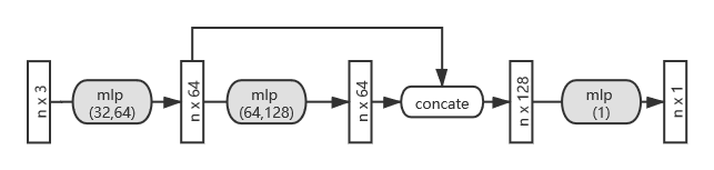
Figure 15: The structure of the network used in our experiments. The input is a matrix of shape $(n,3)$ representing the coordinates of all points in the set, and the output is a matrix of shape $(n,1)$ representing the potential of the corresponding points. $mlp(x)$ represents a multi-layer perceptron (mlp) with the size $x$. For example, $mlp(m,n)$ represents an mlp consisting of two layers, and the size of each layer is $m$ and $n$. We use ReLu activation function in all except the output layer. The activation function ${\bm{l}}(x;h)=\max\{-|x|,-h\}$ is added to the output to clip the output to the interval $[-h,0]$.

We train the network ${\bm{f}}_{w,h}$ using the Adam optimizer [61], and we train the transformation $\mathcal{T}_{\theta}$ using the RMSprop optimizer [62]. The learning rates of both optimizers are set to $10^{-4}$. The parameters are set as follows:

• Experiments in Sec. 5.2.2: For PWAN, we set $(\rho,\lambda,\sigma,T)=(2,0.01,0.1,2000)$; For TPS-RPM, we set $T\_finalfac=500$, $frac=1$, and $T\_init=1.5$; For GMM-REG, we set $sigma=0.5,0.2,0.02$, $Lambda=.1,.02,.01$, $max\_function\_evals=50,50,100$ and $level=3$. For BCPD and CPD, we set $(\beta,\lambda,w)=(2.0,2.0,0.1)$.

• Experiments on the human face dataset: We use m-PWAN with $(\rho,\lambda,\sigma,T)=(0.5,5\times 10^{-4},1.0,3000)$; For BCPD and CPD, we set $(\beta,\lambda,w)=(3.0,20.0,0.1)$.

• Experiments on the human body dataset: We use m-PWAN with $(\rho,\lambda,\sigma,T)=(1.0,1\times 10^{-4},1.0,3000)$; For BCPD and CPD, we set $(\beta,\lambda,w)=(0.3,2.0,0.1)$. We also tried $w=0.6$ but the results are similar (not shown in our experiments).

• Rigid registration: We set $(\beta,\lambda,w)=(2.0,1e^{9},0.1)$ for BCPD. We use the rigid version of the CPD software. We set the same parameter for ICP as PWAN, i.e., we set the distance threshold $d=0.05$ for d-ICP, and set the trimming rate $m=0.8\min(q,r)$ for m-ICP.

The parameters for CPD and BCPD are suggested in [30].

We note that in our experiments, we determine parameter $m$ for m-PWAN by estimating the overlap ratio and setting $m$ as the number of overlapped points. A future direction is to automatically determine the overlap ratio as in [79]. For d-PWAN, we always assume the point sets are uniformly distributed (otherwise we can downsample the point sets using voxel filtering), and set $h$ close to the nearest distance between points in a point set.

B.4 More Details in Sec. 5.2.1

KL divergence and $L_{2}$ distance between point sets $X$ and $Y$ are formally defined as

$$L_{2}(X,Y)=\sum_{\begin{subarray}{c}x_{i},x_{j}\in X\\ y_{i},y_{j}\in Y\end{subarray}}\frac{1}{q^{2}}\phi(0|x_{i}-x_{j},2\sigma) +\frac{1}{r^{2}}\phi(0|y_{i}-y_{j},2\sigma)$$

$$-\frac{2}{qr}\phi(0|x_{i}-y_{j},2\sigma),$$

$$KL(X,Y)=-\frac{1}{q}\sum_{y_{j}\in Y}\log\Bigl{(}\omega\frac{1}{q}+(1-\omega)\sum_{x_{i}\in X}\frac{1}{r}\phi(y_{j}|x_{i},\sigma)\Bigr{)},$$

where $\phi(\cdot|u,\sigma)$ is the Gaussian distribution with mean $u$ and variance $\sigma$. For simplicity, we set $\sigma=1$ and $\omega=0.2$ for KL and $L_{2}$ in Sec. 5.2.1.

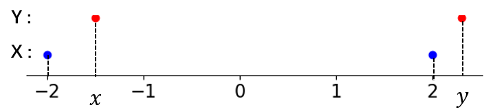
(a) Experimental setting.

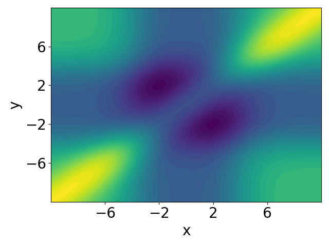
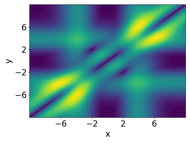
(b) $L_{2}$

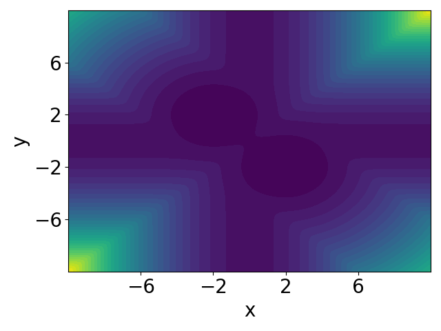
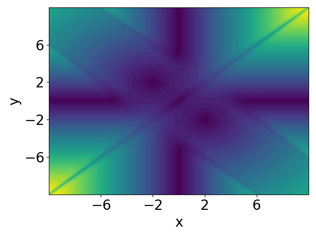
(c) $KL$

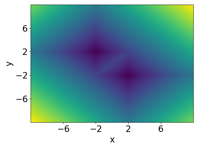
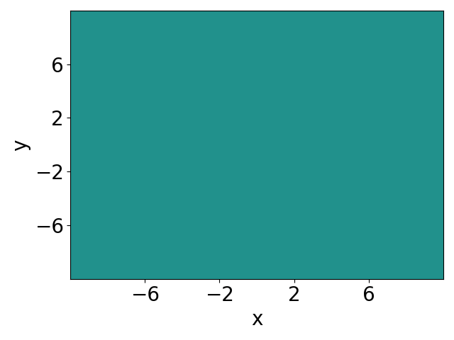
(d) $\mathcal{W}_{1}$

Figure 16: Comparison of different discrepancies on a pair of toy point sets. The top and bottom row in 16(b),16(c) and 16(d) represent the discrepancies and their gradient norms respectively.

We note that compared to KL divergence and $L_{2}$ distance, Wasserstein type divergence is “smoother”, i.e., it can be optimized more easily. To see this, we present a toy example comparing $\mathcal{W}_{1}$, KL divergence and $L_{2}$ distance in Fig. 16. We set $\omega=0$ for KL divergence since the dataset is clean, and we set $\sigma=1$. We fix the reference set $X=\{-2,2\}$, and move the source set $Y=\{x,y\}$ in the 2D space. We present the discrepancies between $X$ and $Y$ as a function of $(x,y)$, and compute their respective gradients.

As can be seen, all discrepancies have two global minima $(-2,2)$ and $(2,-2)$ corresponding to the correct alignment. However, KL divergence has a suspicious stationary point $(0,0)$, which can trap both expectation-maximization-type and gradient-descent-type algorithms [80]. In addition, there exist some regions where the gradient norm of $L_{2}$ distance is small, which indicates optimizing $L_{2}$ may be slow in these regions. In contrast, the gradient norm of $\mathcal{W}_{1}$ is constant, thus the optimization process can easily converge to global minima.

B.5 More Details in Sec. 5.2.2

We present qualitative results of the experiments in Fig. 17 and Fig. 18. We do not show the results of TPS-RPM on the second experiment as it generally fails to converge. As can be seen, PWAN successfully registers the point sets in all cases, while all baseline methods bias toward the noise points or to the non-overlapped region when the outlier ratio is high, except for TPS-RPM which shows strong robustness against noise points comparably with PWAN in the first example.

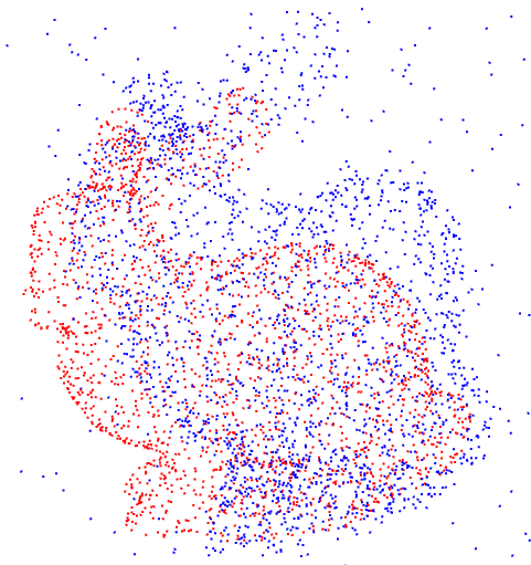
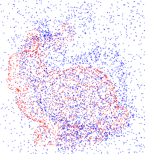
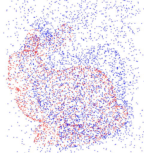
(a) Initial sets

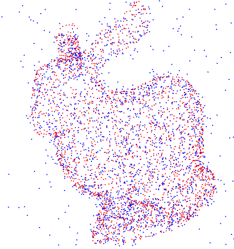
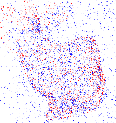
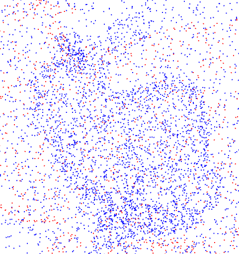
(b) BCPD

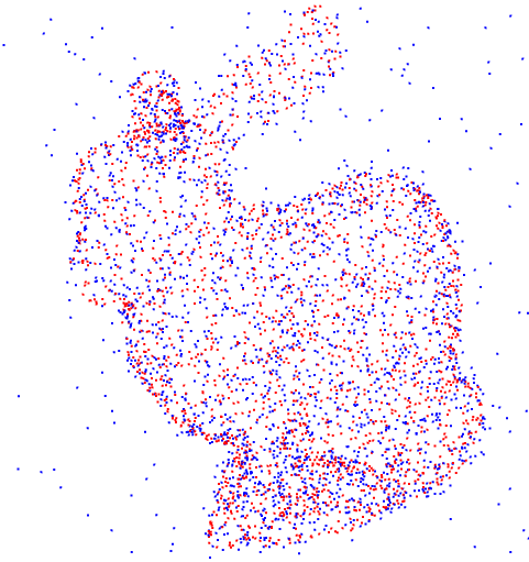
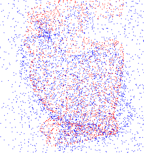
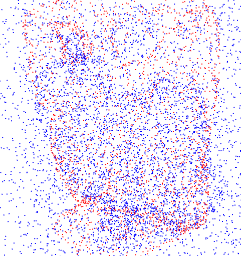
(c) CPD

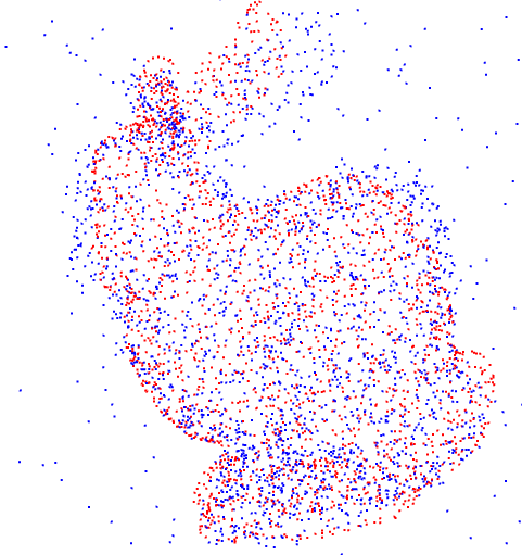
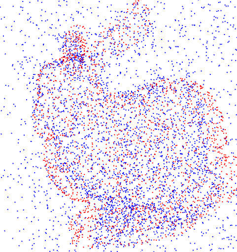
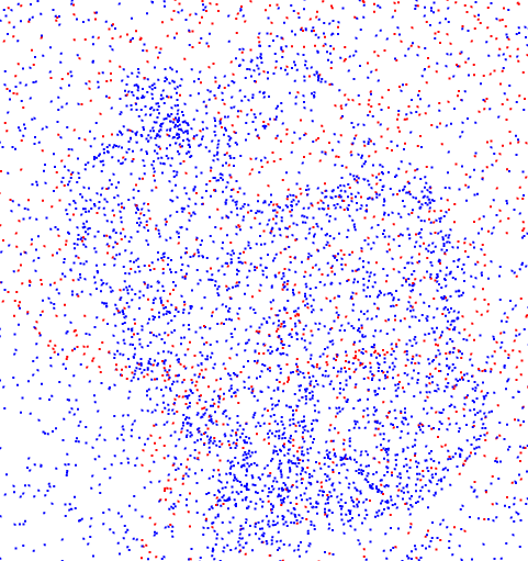
(d) GMM-REG

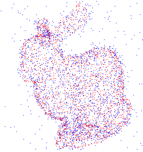
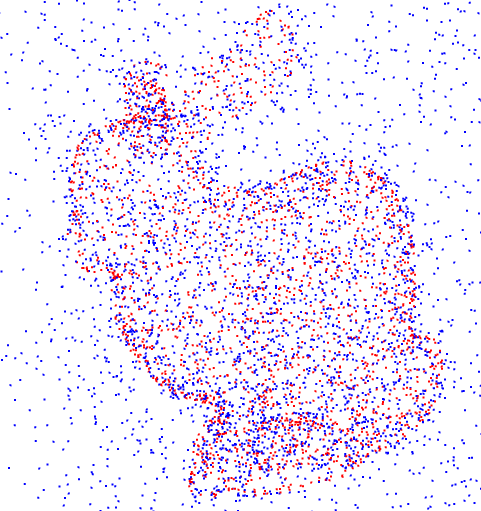
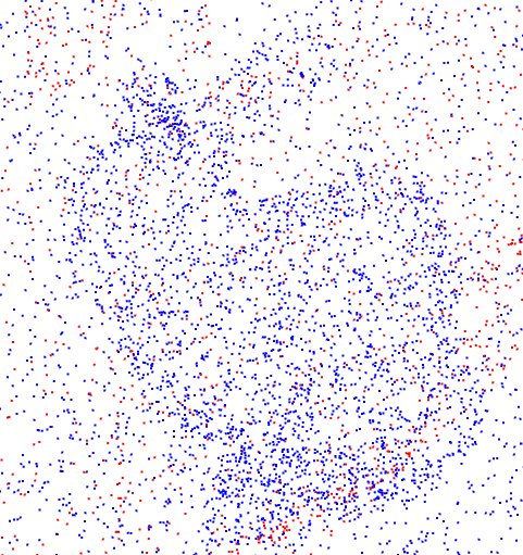
(e) TPS-RPM

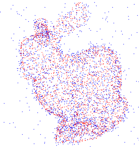
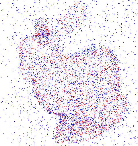
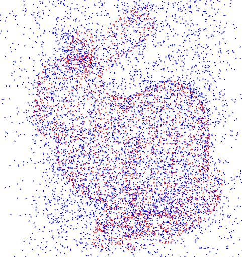
(f) PWAN

Figure 17: An example of registering noisy point sets. The outlier/non-outlier ratios are $0.2$ (1st row), $1.2$ (2nd row) and $2.0$ (3rd row).

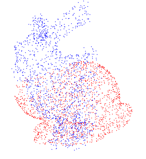
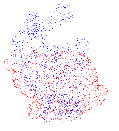
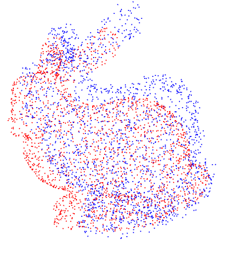
(a) Initial sets

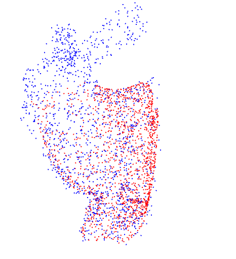
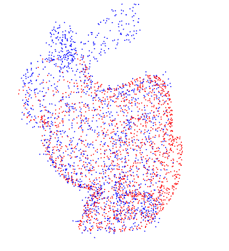
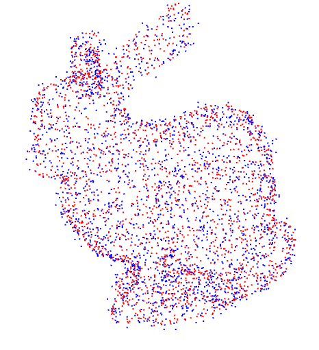
(b) BCPD

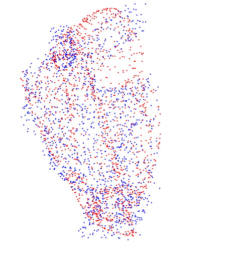
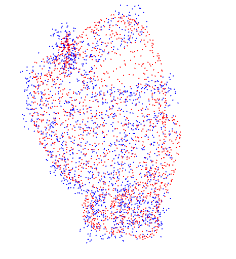
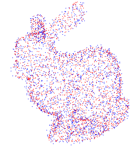
(c) CPD

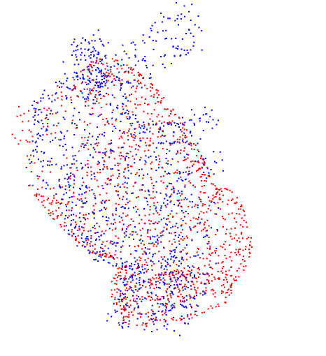
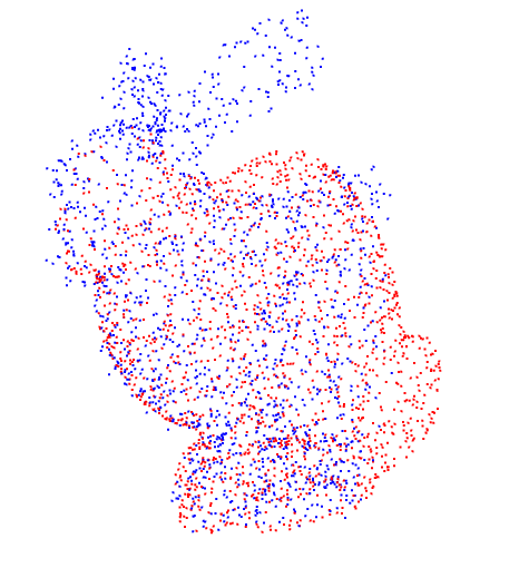
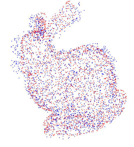
(d) GMM-REG

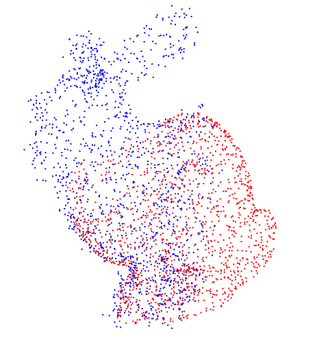
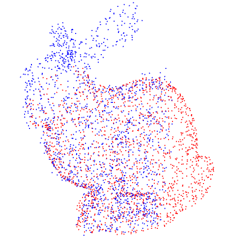
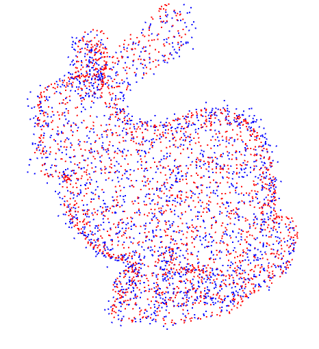
(e) d-PWAN

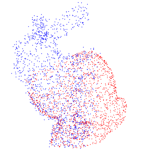
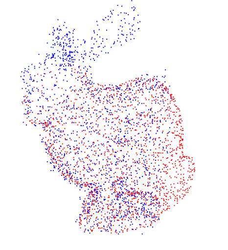
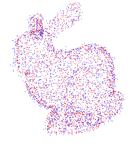
(f) m-PWAN

Figure 18: An example of registering partially overlapped point sets. The overlap ratios are $0.57$ (1st row), $0.75$ (2nd row) and $1$ (3rd row).

We further evaluate PWAN on large-scale armadillo datasets. We compare PWAN with BCPD and CPD, because they are the only baseline methods that are scalable in this experiment. We present some registration results in Fig. 20. As can be seen, our method can handle both cases successfully, while both CPD and BCPD bias toward outliers.

The training details of PWAN in this example are shown in Fig. 21. Due to its adversarial nature, the loss of PWAN does not decrease monotonically, instead, it always increases during the first few steps, and then starts to decrease. In addition, the maximal gradient norm of the network (Lipschitz constant) is indeed controlled near $1$, and the MSE decreases during the training process. An example of the registration process is presented in Fig. 19(a).

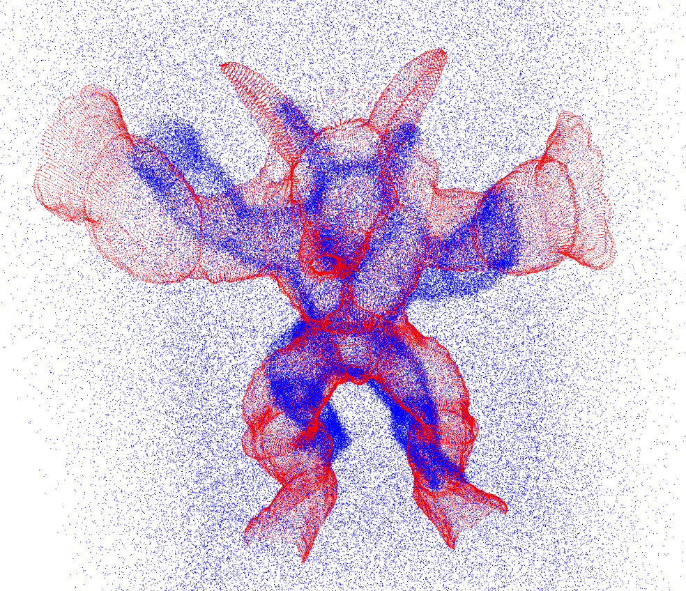
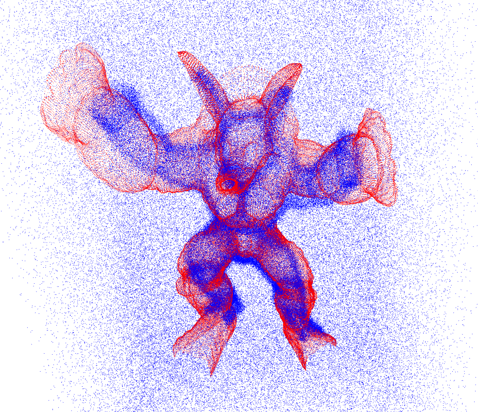
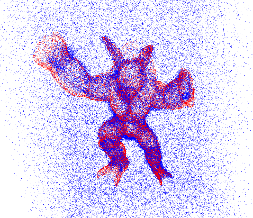
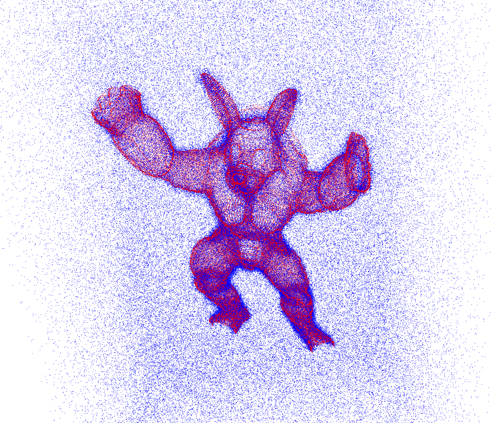
(a) A trajectory of non-rigid registration of the armadillo dataset.

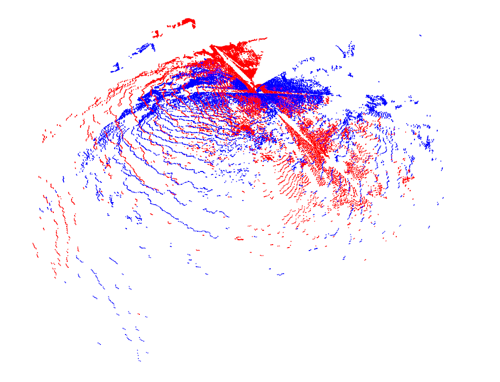
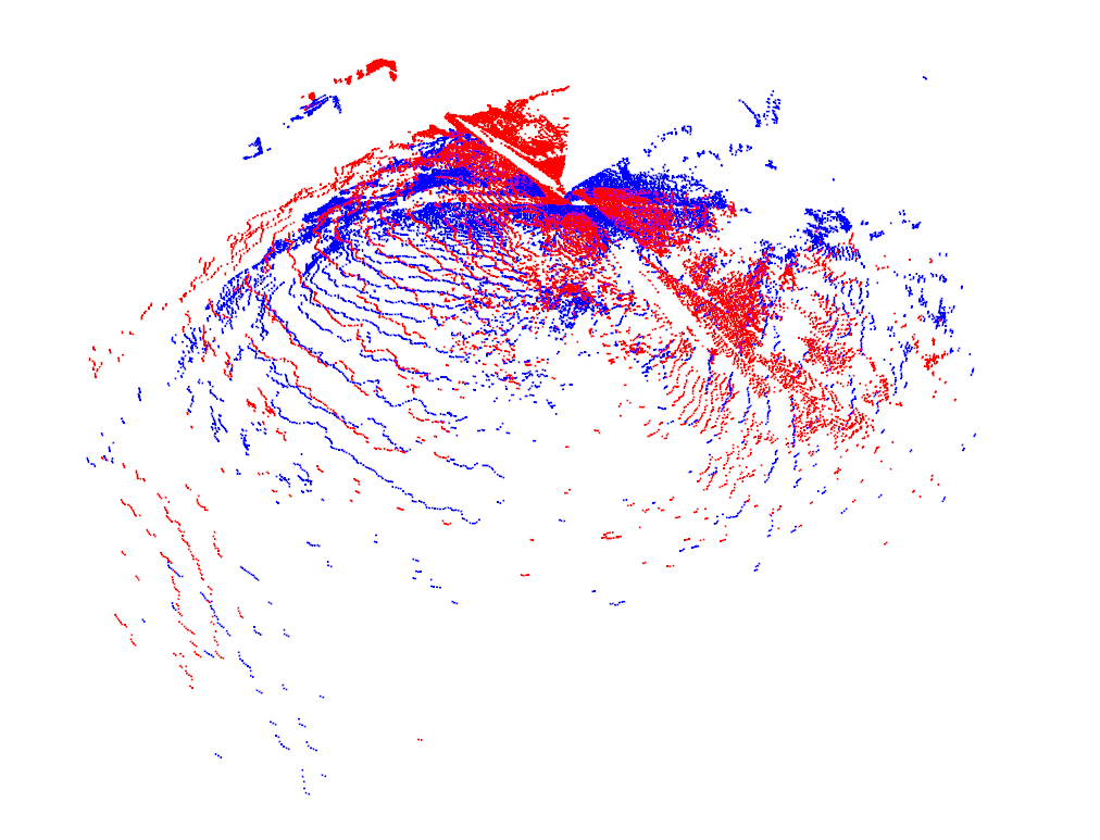
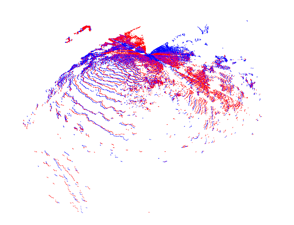
(b) A trajectory of rigid registration of the mountain dataset.

Figure 19: Registration trajectory. We show the process of non-rigid 19(a) and rigid registration 19(b) from left to right.

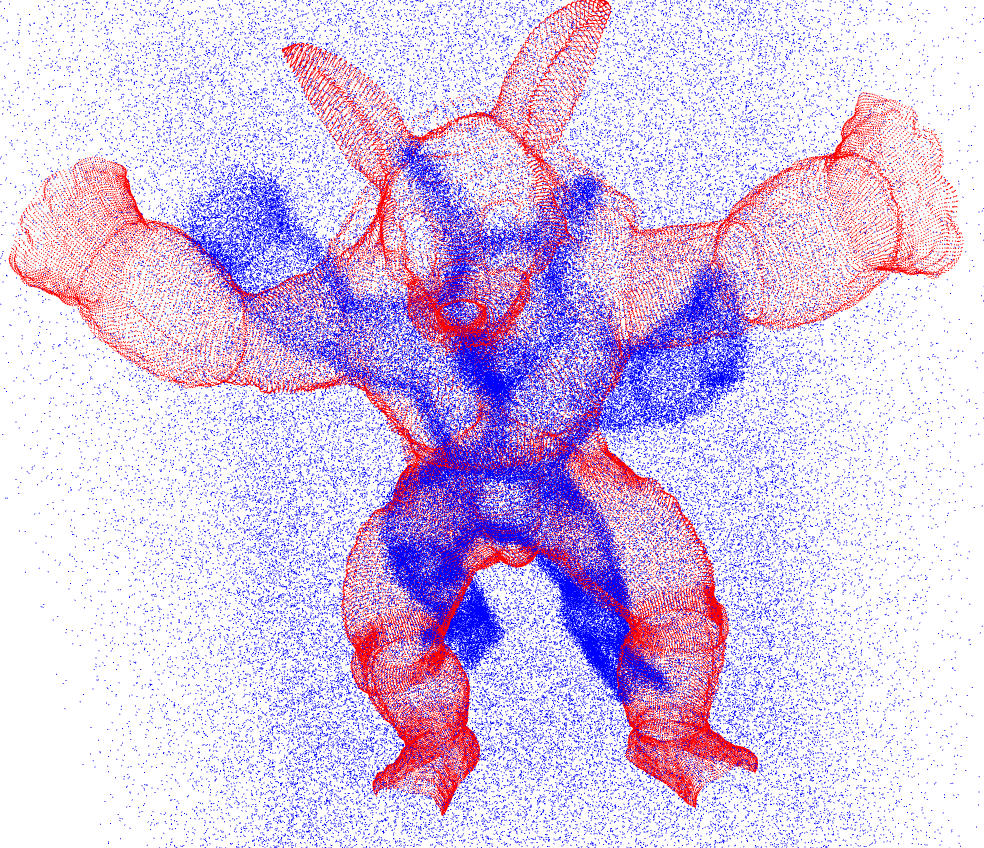
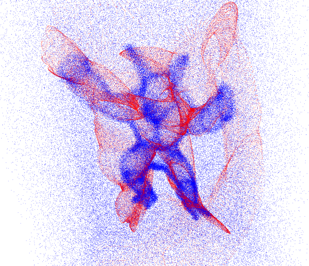
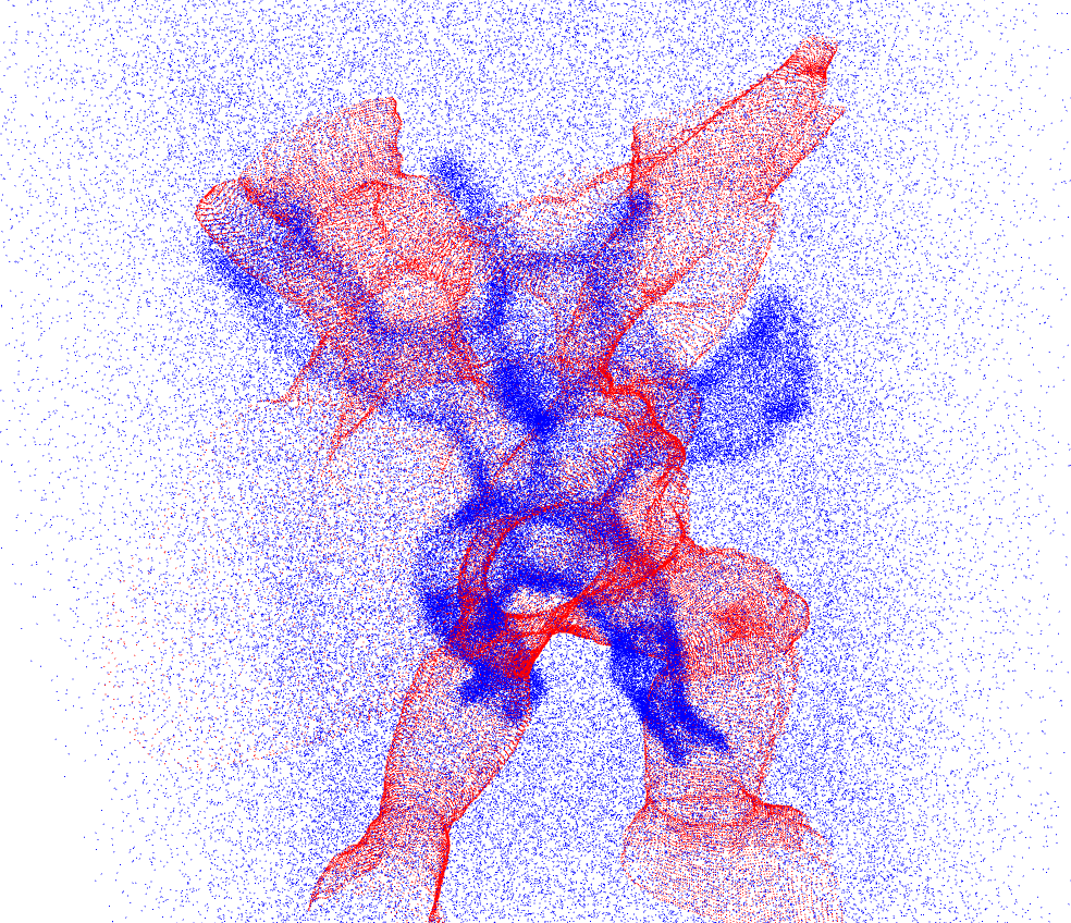
Initial sets                      BCPD                         CPD                      PWAN

(a) An example of registering noisy point sets. The source and reference set contain $8\times 10^{4}$ and $1.76\times 10^{5}$ points respectively.

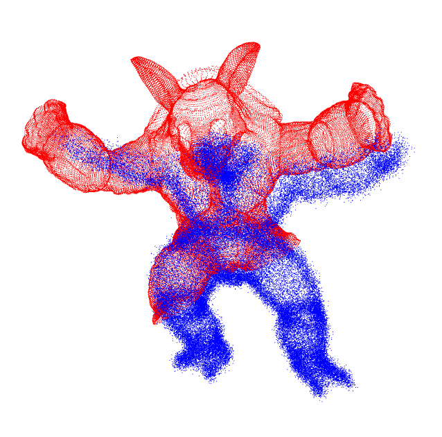
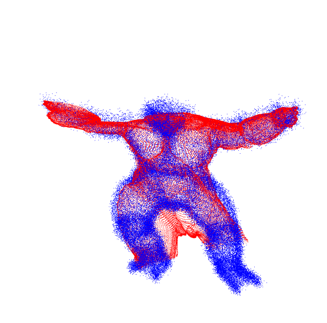
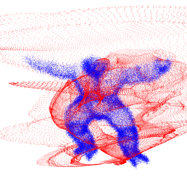
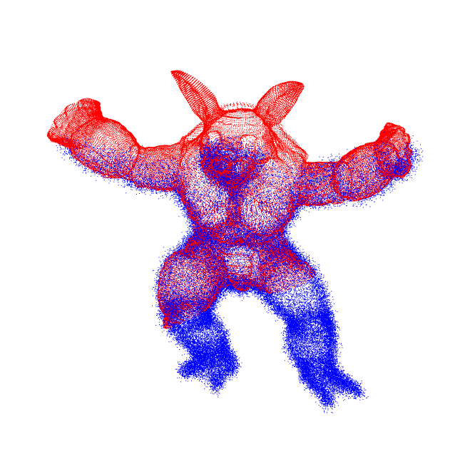
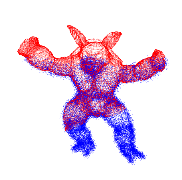
Initial sets                   BCPD                      CPD                    d-PWAN                   m-PWAN

(b) An example of registering partially overlapped point sets. The source and reference set both contain $7\times 10^{4}$ points.

Figure 20: Examples of registering large-scale point sets.

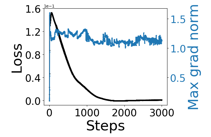
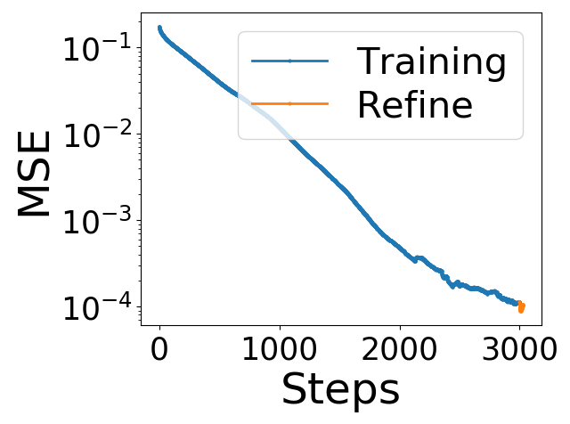
Figure 21: Training details of PWAN on the pair of point sets shown in Fig. 20(a)

B.6 More Details in Sec. 5.2.4

The quantitative comparison on human face datasets is presented in Tab. VI.

TABLE VI: Quantitative result of registering the space-time faces dataset.

	BCPD	CPD	PWAN
MSE $(\times 10^{-3})$	1.7 (1.0)	0.49 (0.2)	0.32 (0.08)

The human body dataset is taken from a SHREC’19 track called “matching humans with different connectivity” [49]. This dataset consists of $44$ shapes, and we manually select $3$ pairs of shapes for our experiments. To generate a point set for a shape, we first sample $50000$ random points from the 3D mesh, and then apply voxel grid filtering to down-sample the point set to less than $10000$ points. The description for the generated point sets is presented in Tab. VII

TABLE VII: Point sets used for registration. no.$m$ represents the m-th shape in the dataset [49].

	(no.1, no.42)	(no.18, no.19)	(no.30, no.31)
Size	(5575, 5793)	(6090, 6175)	(6895, 6792)
Description	same pose different person	different pose same person	different pose different person

We conduct two experiments to evaluate PWAN on registering complete and incomplete point sets respectively. In the first experiment, we register $3$ pairs of point sets using PWAN, where the human shapes come from different people or/and with different poses. In the second experiment, we register incomplete point sets which are generated by cropping a fraction of the no.30 and no.31 point sets. For both experiments, we compare PWAN with CPD [10] and BCPD [30], and we only present qualitative registration results, because we do not know the true correspondence between point sets.

The results of the first experiment are shown in Fig. 22. As can be seen, PWAN can handle articulated deformations and produce good full-body registration results. In contrast, CPD and BCPD have difficulties aligning point sets with large articulated deformations, as significant registration errors are observed near the limbs.

The results of the second experiment are shown in Fig. 23. As can be seen, both CPD and BCPD fail in this experiment, as the non-overlapping points are seriously biased. For example, in the $3$-rd row, they both wrongly match the left arm to the body, which causes highly unnatural artifacts. In contrast, the proposed PWAN can handle the partial matching problem well, since it successfully maintains the shape of non-overlapping regions, which contributes to the natural registration results.

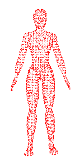
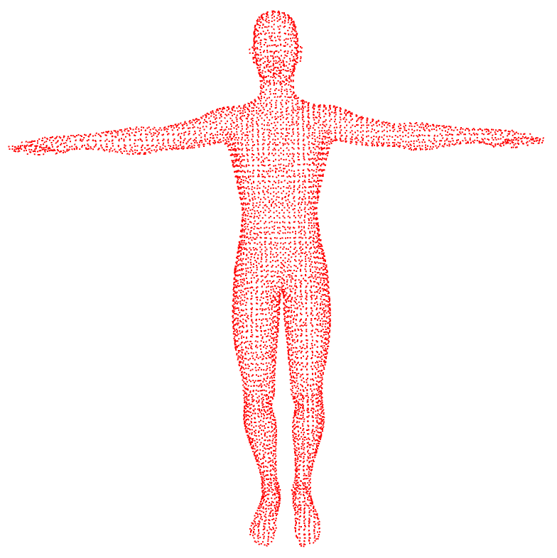
(a) Source set

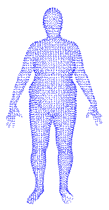
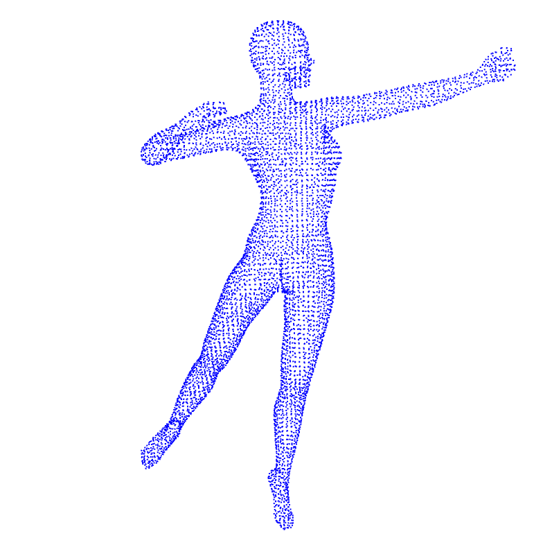
(b) Reference set

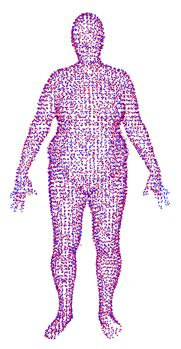
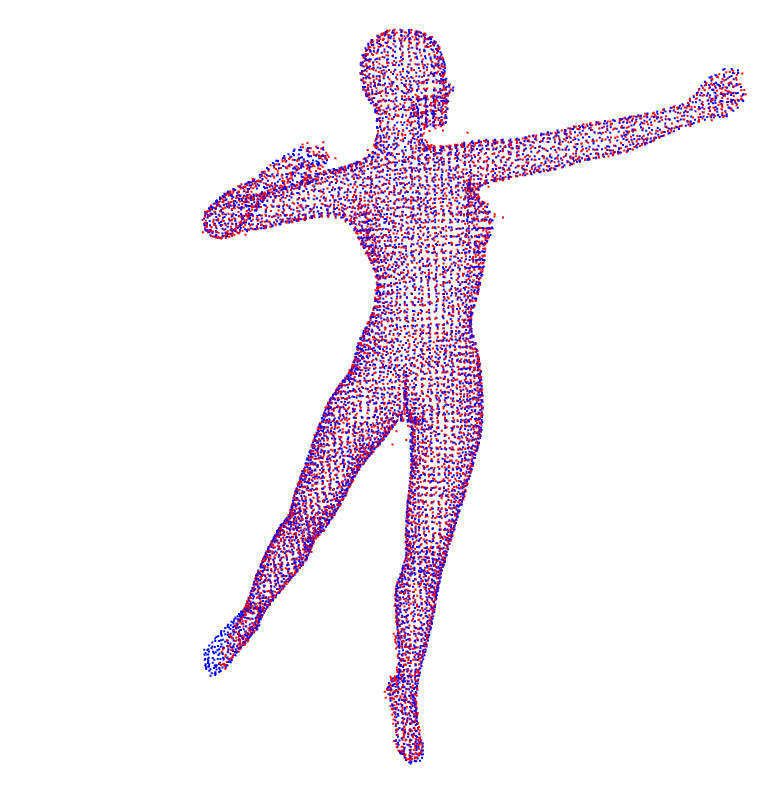
(c) PWAN (Ours)

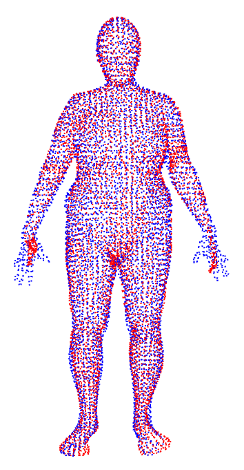
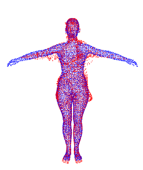
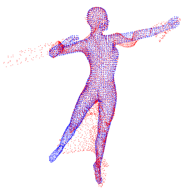
(d) BCPD [30]

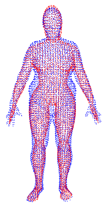
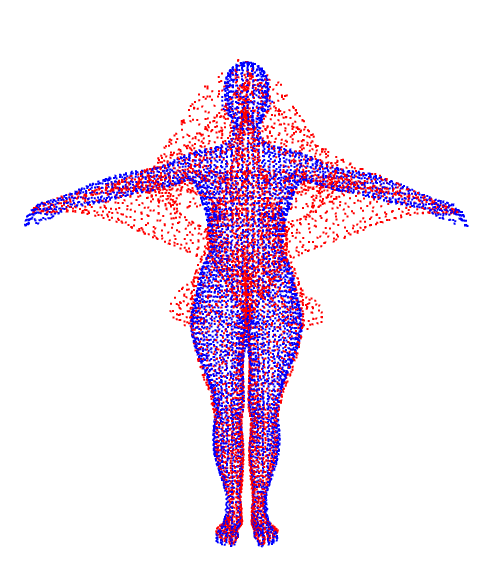
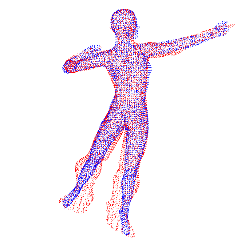
(e) CPD [10]

Figure 22: The results of registering complete point sets no.1 to no.42 (1-st row), no.18 to no.19 (2-nd row), and no.30 to no.31 (3-rd row).

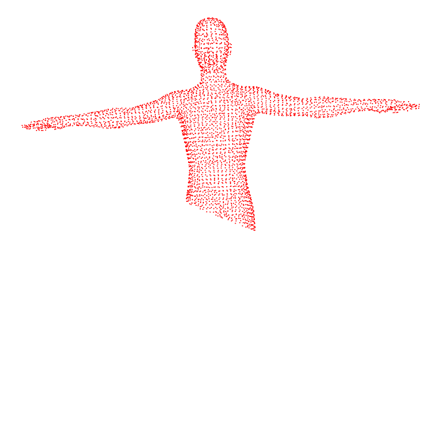
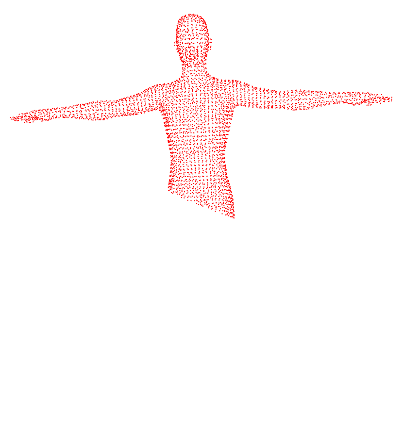
(a) Source set

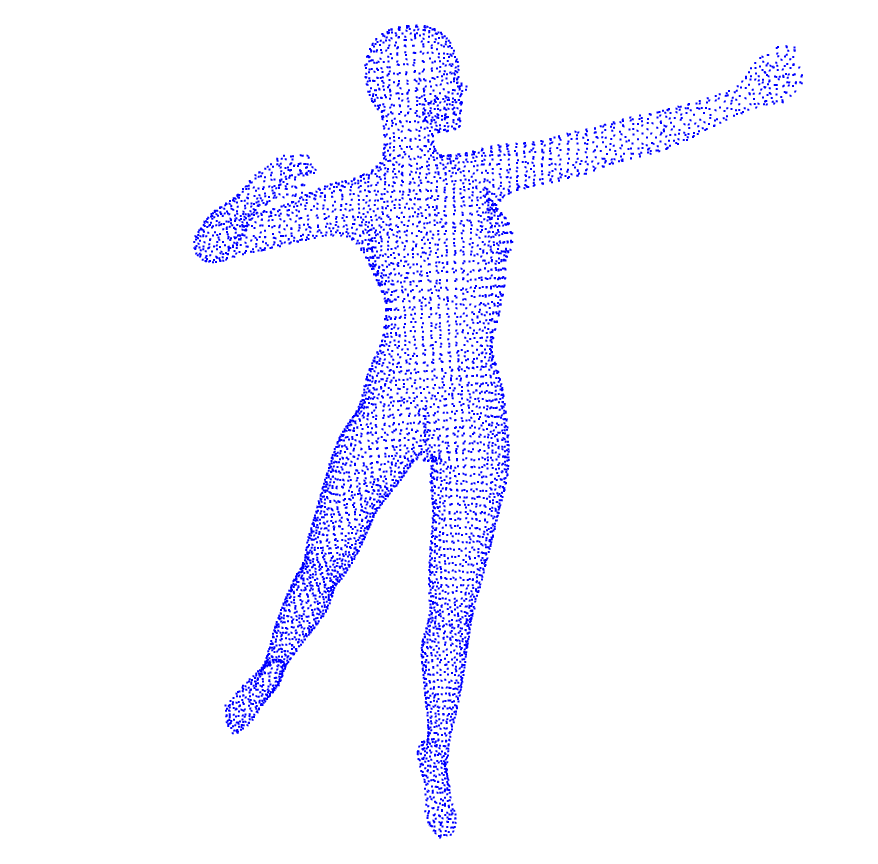
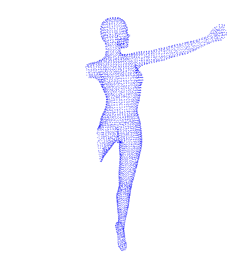
(b) Reference set

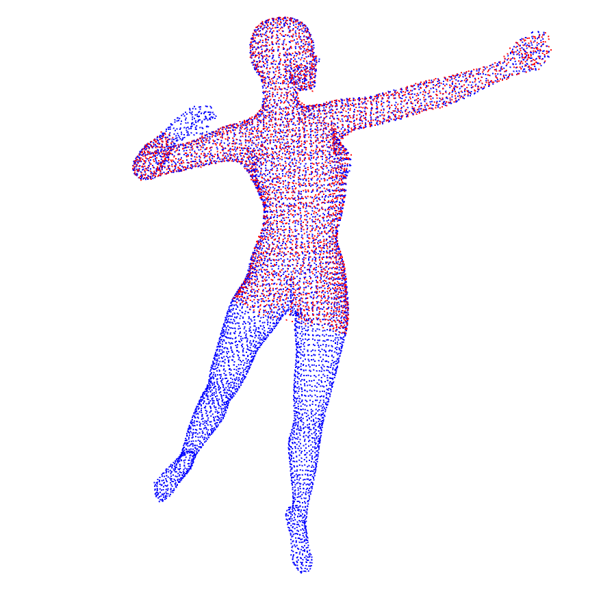
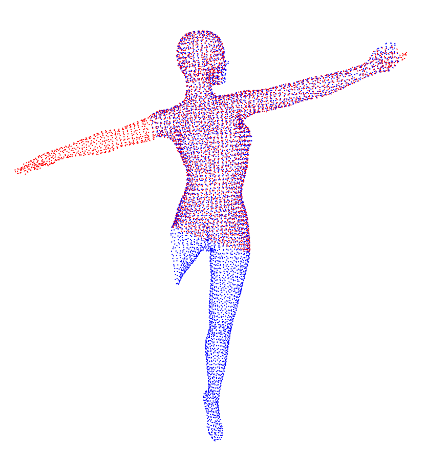
(c) PWAN (Ours)

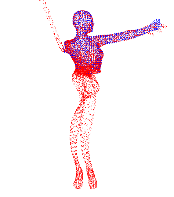
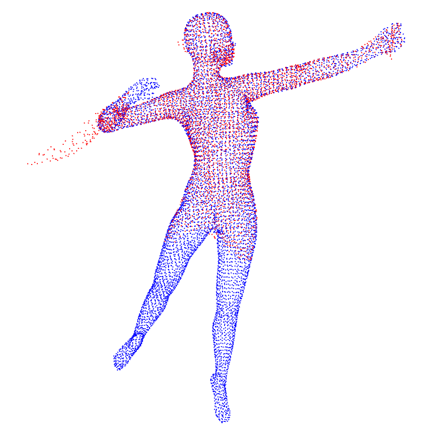
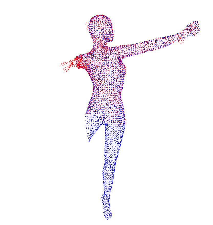
(d) BCPD [30]

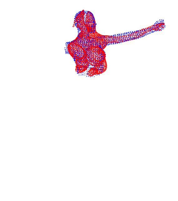
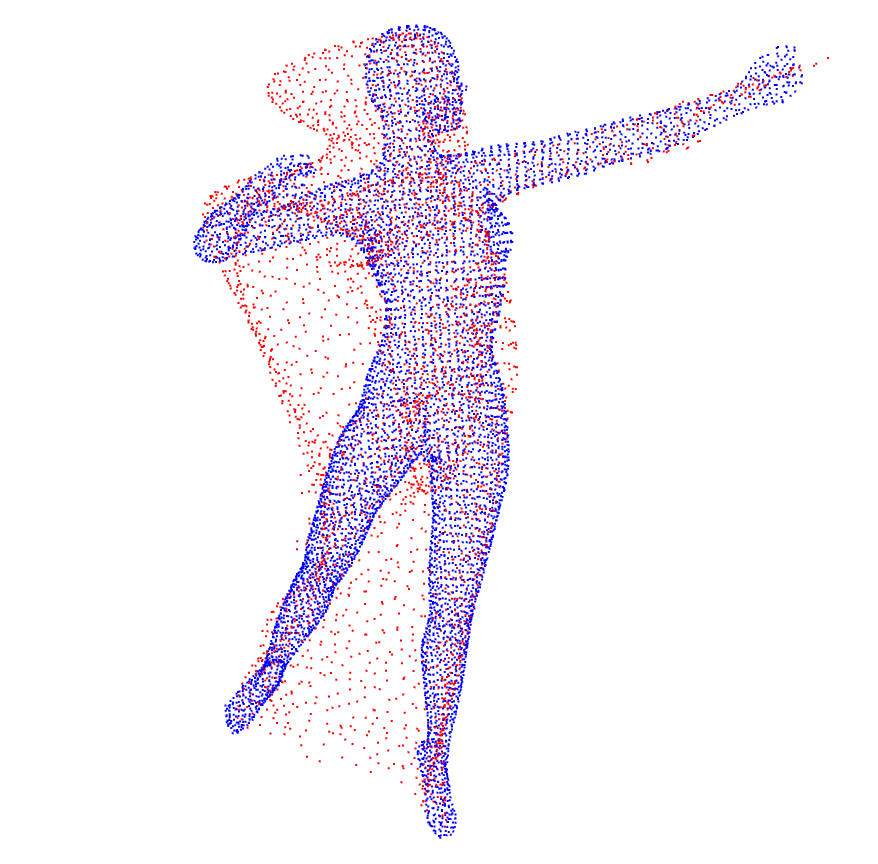
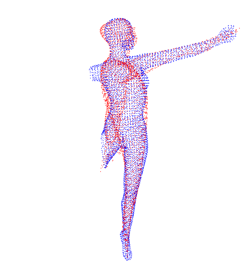
(e) CPD [10]

Figure 23: Registering incomplete point sets no.30 to no.31. We present the results of complete-to-incomplete (1-st row), incomplete-to-complete (2-nd row) and incomplete-to-incomplete (3-rd row) registration.

B.7 More Details in Sec. 5.2.5

The detailed quantitative results of rigid registration are presented in Tab. VIII, and we additionally present some examples of the registration results in Fig. 24. It can be seen that both types of PWAN can accurately align all point sets, while all baseline algorithms failed to handle the parasaurolophus shapes.

TABLE VIII: Quantitative results of rigid registration. We report the median and standard deviation of rotation errors.

	apartment	mountain	stair	wood-summer	parasaurolophus	T-rex
BCPD	0.71 (13.4)	8.07 (7.4)	0.24 (3.8)	7.32 (9.4)	0.16 (0.2)	0.09 (0.2)
CPD	0.50 (1.7)	6.39 (3.6)	0.9 (39.2)	1.99 (1.6)	0.17 (60.8)	0.08 (63.2)
m-ICP	1.86 (28.9)	11.23 (13.9)	0.32 (2.3)	11.29 (7.9)	1.94 (8.1)	1.85 (2.5)
d-ICP	11.14 (23.2)	13.44 (6.1)	3.92 (6.4)	23.68 (8.2)	21.29 (8.1)	21.05 (4.2)
m-PWAN (Ours)	0.32 (19.5)	4.67 (4.1)	0.23 (0.2)	1.17 (0.8)	0.11 (0.4)	0.10 (0.1)
d-PWAN (Ours)	0.36 (29.9)	4.7 (4.1)	0.23 (0.2)	1.20 (0.8)	0.12 (2.3)	0.07 (7.4)

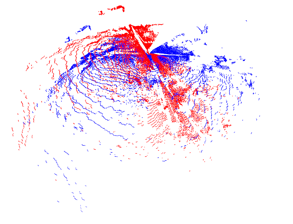
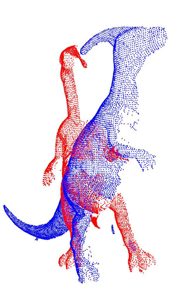
(a) Initial sets

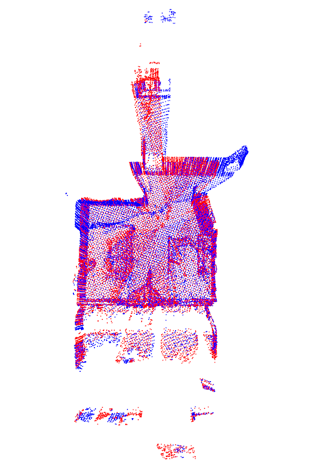
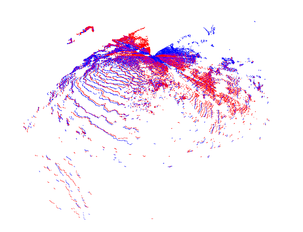
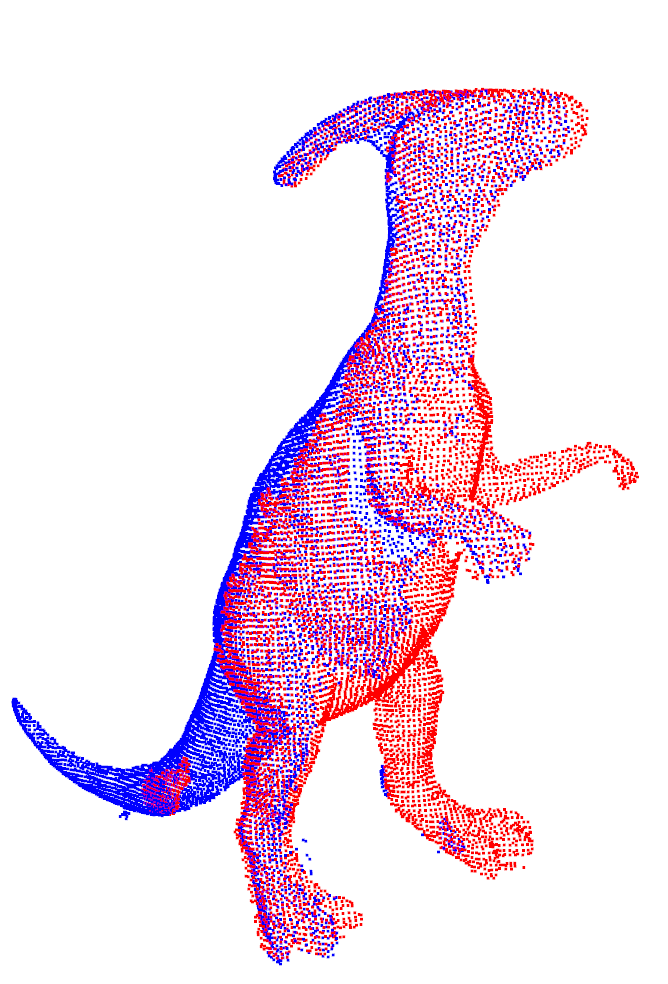
(b) d-PWAN

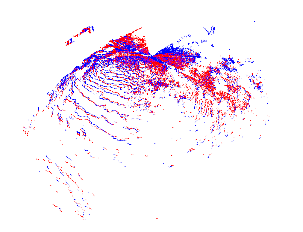
(c) m-PWAN

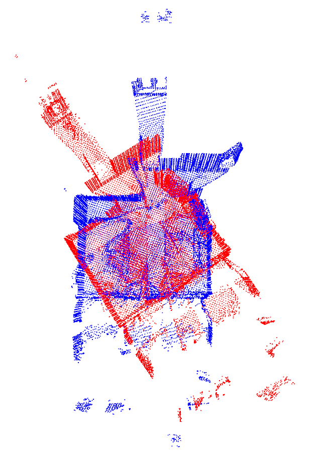
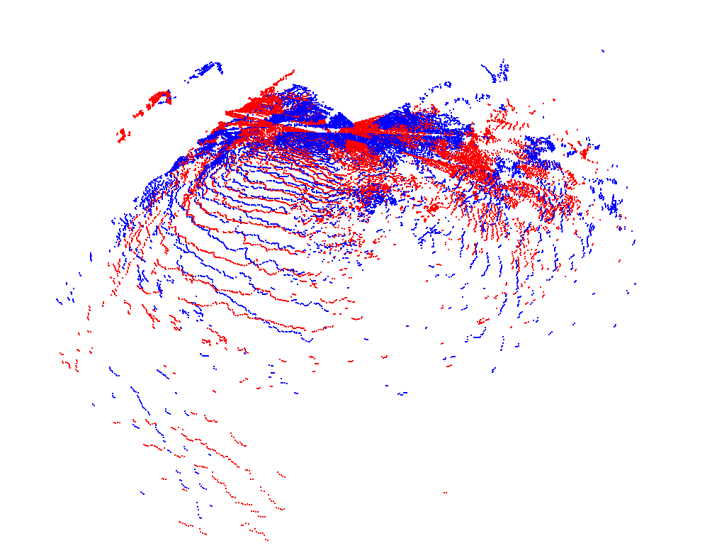
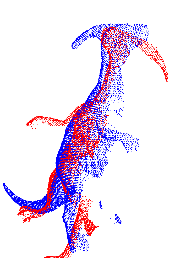
(d) BCPD

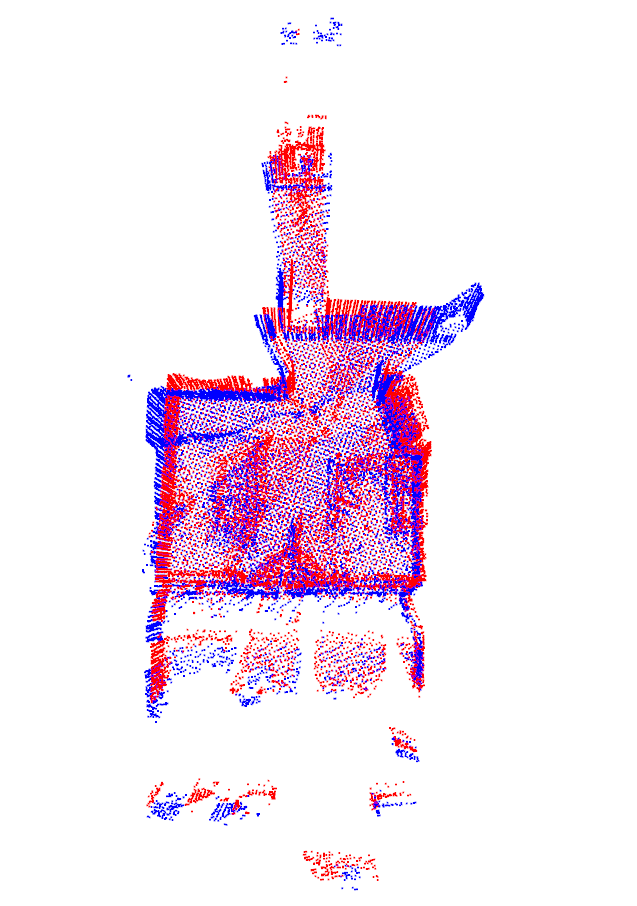
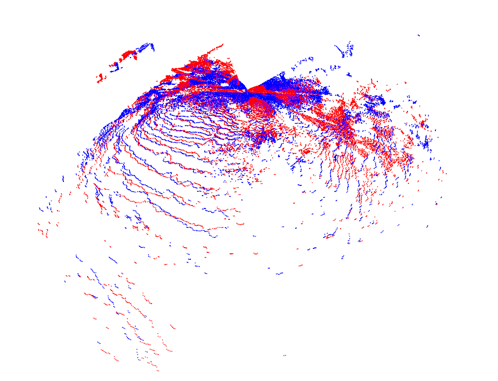
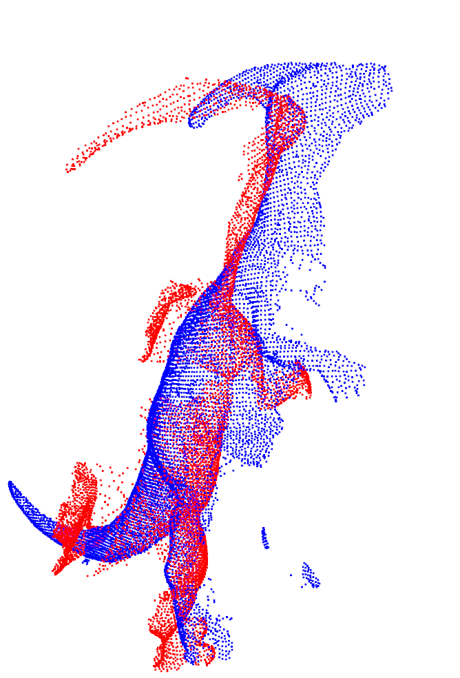
(e) CPD

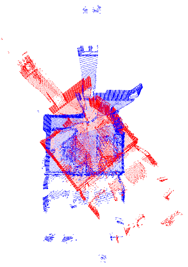
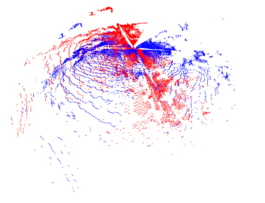
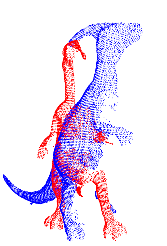
(f) d-ICP

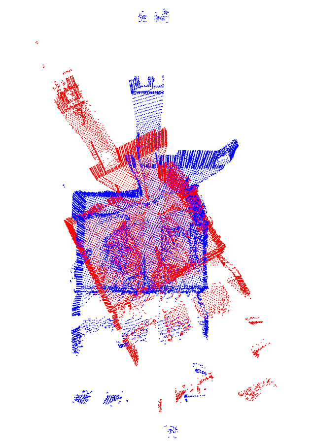
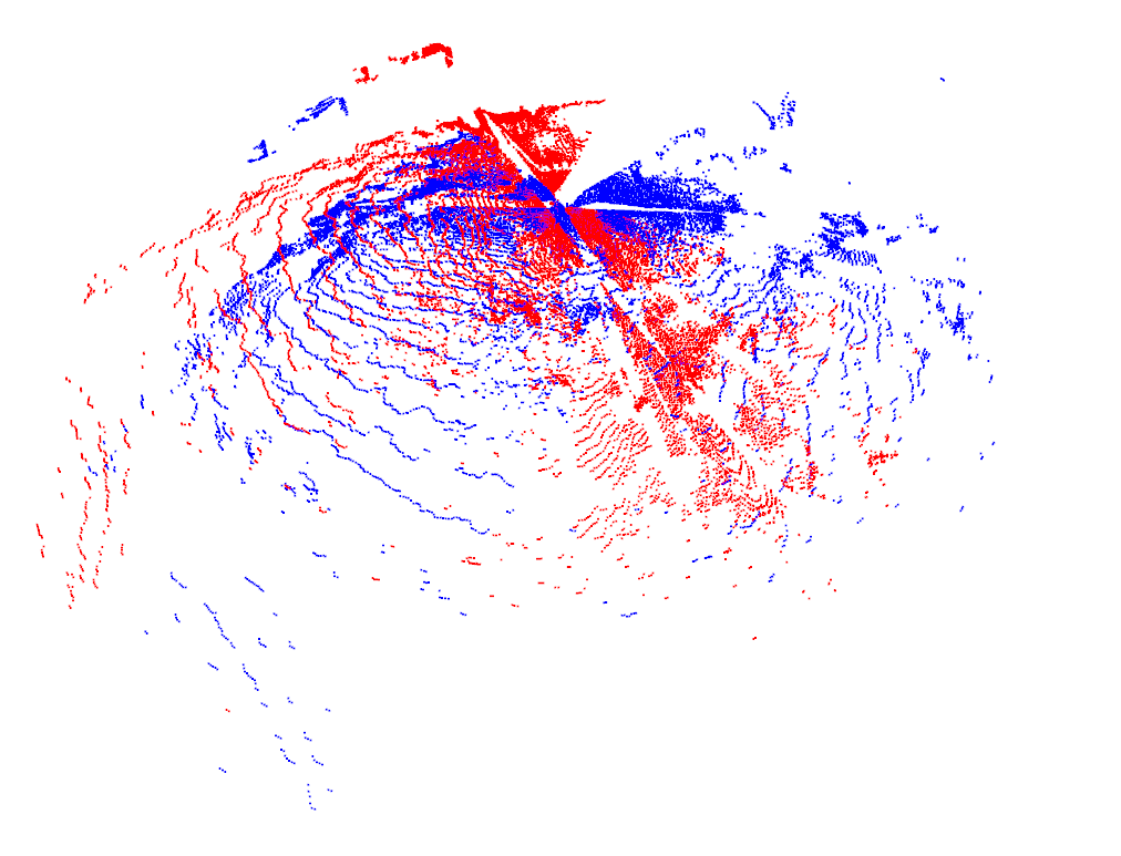
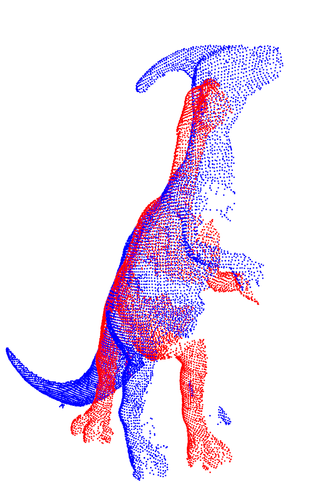
(g) m-ICP

Figure 24: Examples of rigid registration results on a pair of apartment (indoor), mountain (outdoor) and parasaurolophus (object) point sets.

B.8 Explanation of the Effect of $m_{\alpha}$

To explain the effect of $m_{\alpha}$ in our formulation, we present a toy example in Fig. 25, where $\alpha$ and $\beta_{\theta}$ are uniform distributions supported on points. We consider the correspondence given by $\mathcal{L}_{M,1}(\alpha,\beta_{\theta})$, where we fix $m_{\beta}=1$ and increase $m_{\alpha}$ from $1$ to infinity. Fewer data points in $\alpha$ are aligned as $m_{\alpha}$ increases, and the alignment gradually becomes the nearest neighborhood alignment when $m_{\alpha}$ is close to infinity.

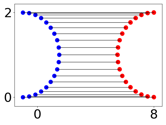
(a) $m_{\alpha}=1$

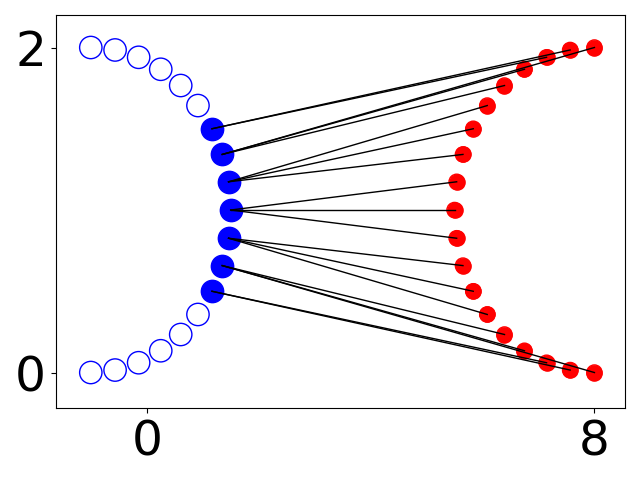
(b) $m_{\alpha}=3$

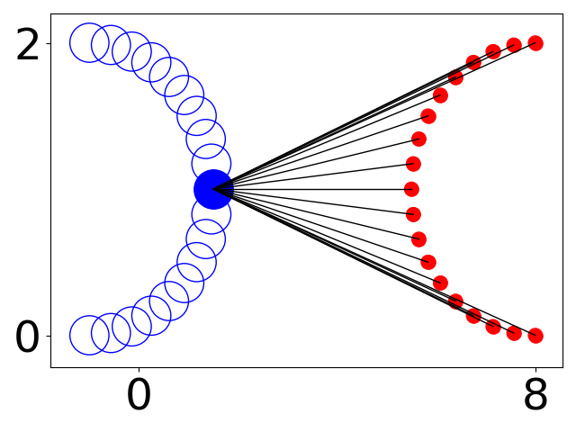
(c) $m_{\alpha}=20$

Figure 25: The alignment of $\alpha$ (blue) and $\beta_{\theta}$ (red) specified by $\mathcal{L}_{M,1}(\alpha,\beta_{\theta})$ with $m_{\beta}=1$ and varying $m_{\alpha}$. The size of each point is proportional to its mass. Complete alignment ($m_{\alpha}=1$) gradually becomes the nearest neighborhood alignment ($m_{\alpha}=\infty$) as $m_{\alpha}$ increases.

B.9 Detailed Experimental Settings in Sec. 6.2

The parameters of PWAN are set as follows:

• Office-Home: The batch size is $65$ and we use a stratified sampler as in [81], i.e., a mini-batch contains $1$ random sample from each reference class. We set $(T,u,s)=(5\times 10^{3},5,10^{3/10000})$.

• VisDa17: We use batch size $60$ and a stratified sampler. $(T,u,s)=(10^{4},20,10^{5/10000})$.

• ImageNet-Caltech: We use batch size $100$. $(T,u,s)=(4.8\times 10^{4},1,10^{1/48000})$.

• DomainNet: We use batch size $100$. $(T,u,s)=(10^{4},1,10^{6/100000})$. Following [38], for this dataset, we do not use Relu activation function at the bottleneck layer.

In the above settings, we select the largest possible batch size to fit in the GPU memory for each task, and sufficiently long training steps are chosen to make sure PWAN converges. We evaluate all methods by their test accuracy at the end of the training instead of the highest accuracy during the training [38]. In our experiments, the bottleneck size of ADV [38] is reduced to $512$ from $2048$ for ImageNet-Caltech to prevent the out-of-memory error.

B.10 More Details in Sec. 6.2.3

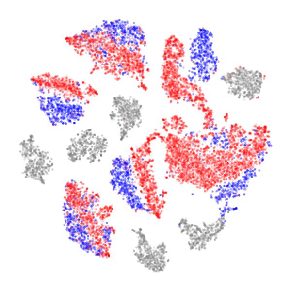
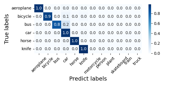
(a) The result of PWAN with random seed $0$. (Accuracy=$94\%$)

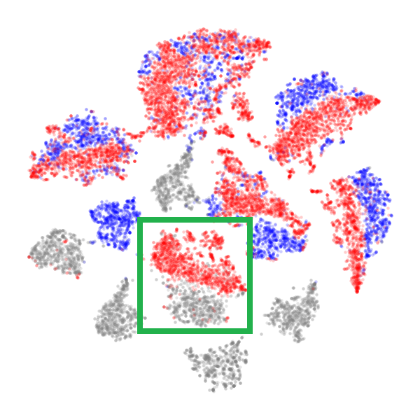
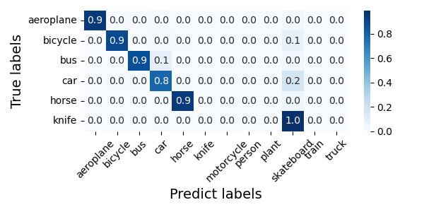
(b) The result of PWAN with random seed $1$. (Accuracy=$80\%$)

(c) Random samples of the knife class in the source domain.

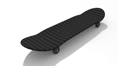
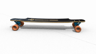
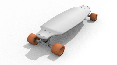
(d) Random samples of the skateboard class in the reference domain.

Figure 26: The results of PWAN on VisDa17. PWAN sometimes has difficulty discriminating the “skateboard” and the “knife” class due to their visual similarity. In practice, this issue can be easily solved by model selection using a small annotated validation set.

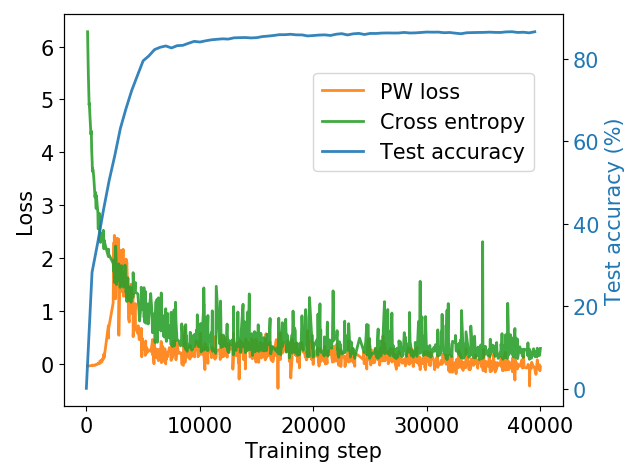
Figure 27: The training process of PWAN on ImageNet-Caltech. PW loss and cross-entropy loss gradually decrease until convergence. Meanwhile, test accuracy increases during the training process.

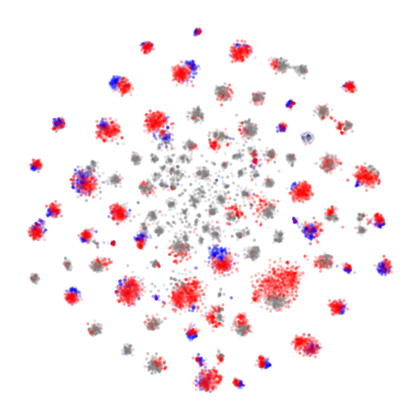
(a) CP-DomainNet

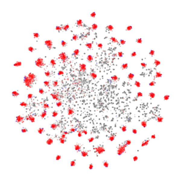
(b) ImageNet-Caltech

Figure 28: t-SNE visualization of the learned features of PWAN. Blue and gray points represent features in non-outlier and outlier classes in the reference domain respectively. Red points represent features in the source domain.

We provide more details of the result of PWAN on VisDa17 in Fig. 26. We observe that PWAN generally performs well on all classes, except that it sometimes recognizes the “knife” class as the “skateboard” classes as shown in Fig. 26(a) and Fig. 26(b). This error is somehow reasonable because these two classes are visually similar as shown in i.e., Fig. 26(c) and Fig. 26(d). We argue that this ambiguity can be easily addressed in real applications, as we can choose the high-performance model by testing the model on a small annotated validation set. In addition, compared to the results in Fig.8 in [11], PWAN achieves much better results, as it can easily discriminate classes “bicycle”/“motorcycle” and “bus”/“car”/“train”.

The training process on ImageNet-Caltech dataset is presented in Fig. 27, where both cross-entropy and PW divergence converge during the training process. In addition, we provide a visualization of the learned features on ImageNet-Caltech and DomainNet in Fig. 28, where PWAN successfully aligns the source features to the reference features even when the reference data is dominated by outliers ($68\%$ of classes of DomainNet and $92\%$ of classes of ImageNet-Caltech are outliers).

References

- [1] M. Arjovsky, S. Chintala, and L. Bottou, “Wasserstein generative adversarial networks,” in Proceedings of the 34th International Conference on Machine Learning, ser. Proceedings of Machine Learning Research, D. Precup and Y. W. Teh, Eds., vol. 70. PMLR, 06–11 Aug 2017, pp. 214–223.
- [2] Y. Song and S. Ermon, “Generative modeling by estimating gradients of the data distribution,” Advances in neural information processing systems, vol. 32, 2019.
- [3] J. Ho, A. Jain, and P. Abbeel, “Denoising diffusion probabilistic models,” Advances in neural information processing systems, vol. 33, pp. 6840–6851, 2020.
- [4] L. Chizat, G. Peyré, B. Schmitzer, and F.-X. Vialard, “Scaling algorithms for unbalanced optimal transport problems,” Mathematics of Computation, vol. 87, no. 314, pp. 2563–2609, 2018.
- [5] L. Chapel, M. Z. Alaya, and G. Gasso, “Partial optimal tranport with applications on positive-unlabeled learning,” Advances in Neural Information Processing Systems, vol. 33, pp. 2903–2913, 2020.
- [6] D. Mukherjee, A. Guha, J. M. Solomon, Y. Sun, and M. Yurochkin, “Outlier-robust optimal transport,” in International Conference on Machine Learning. PMLR, 2021, pp. 7850–7860.
- [7] C. Villani, Optimal transport: old and new. Springer, 2009, vol. 338.
- [8] A. Figalli, “The optimal partial transport problem,” Archive for Rational Mechanics and Analysis, vol. 195, no. 2, pp. 533–560, 2010.
- [9] C. Villani, Topics in optimal transportation. American Mathematical Soc., 2003, no. 58.
- [10] A. Myronenko and X. Song, “Point set registration: Coherent point drift,” IEEE Transactions on Pattern Analysis and Machine Intelligence, vol. 32, no. 12, pp. 2262–2275, 2010.
- [11] Z. Cao, K. You, Z. Zhang, J. Wang, and M. Long, “From big to small: adaptive learning to partial-set domains,” IEEE Transactions on Pattern Analysis and Machine Intelligence, vol. 45, no. 2, pp. 1766–1780, 2022.
- [12] Z. Cao, L. Ma, M. Long, and J. Wang, “Partial adversarial domain adaptation,” in Proceedings of the European conference on computer vision (ECCV), 2018, pp. 135–150.
- [13] Z.-M. Wang, N. Xue, L. Lei, and G.-S. Xia, “Partial wasserstein adversarial network for non-rigid point set registration,” in International Conference on Learning Representations (ICLR), 2022.
- [14] L. A. Caffarelli and R. J. McCann, “Free boundaries in optimal transport and monge-ampere obstacle problems,” Annals of Mathematics, vol. 171, no. 2, pp. 673–730, 2010.
- [15] A. Makkuva, A. Taghvaei, S. Oh, and J. Lee, “Optimal transport mapping via input convex neural networks,” in International Conference on Machine Learning. PMLR, 2020, pp. 6672–6681.
- [16] B. Schmitzer, “Stabilized sparse scaling algorithms for entropy regularized transport problems,” SIAM Journal on Scientific Computing, vol. 41, no. 3, pp. A1443–A1481, 2019.
- [17] N. Bonneel, J. Rabin, G. Peyré, and H. Pfister, “Sliced and radon wasserstein barycenters of measures,” Journal of Mathematical Imaging and Vision, vol. 51, no. 1, pp. 22–45, 2015.
- [18] B. Schmitzer and B. Wirth, “A framework for wasserstein-1-type metrics,” Journal of Convex Analysis, vol. 26, no. 2, pp. 353–396, 2019.
- [19] J.-D. Benamou, G. Carlier, M. Cuturi, L. Nenna, and G. Peyré, “Iterative bregman projections for regularized transportation problems,” SIAM Journal on Scientific Computing, vol. 37, no. 2, pp. A1111–A1138, 2015.
- [20] M. Cuturi, “Sinkhorn distances: Lightspeed computation of optimal transport,” in Advances in neural information processing systems, 2013, pp. 2292–2300.
- [21] K. Fatras, T. Séjourné, R. Flamary, and N. Courty, “Unbalanced minibatch optimal transport; applications to domain adaptation,” in International Conference on Machine Learning. PMLR, 2021, pp. 3186–3197.
- [22] K. Fatras, Y. Zine, R. Flamary, R. Gribonval, and N. Courty, “Learning with minibatch wasserstein: asymptotic and gradient properties,” in AISTATS 2020-23nd International Conference on Artificial Intelligence and Statistics, vol. 108, 2020, pp. 1–20.
- [23] K. Nguyen, D. Nguyen, T. Pham, N. Ho et al., “Improving mini-batch optimal transport via partial transportation,” in International Conference on Machine Learning. PMLR, 2022, pp. 16 656–16 690.
- [24] J. Lellmann, D. A. Lorenz, C.-B. Schönlieb, and T. Valkonen, “Imaging with kantorovich–rubinstein discrepancy,” Siam Journal on Imaging Sciences, vol. 7, no. 4, pp. 2833–2859, 2014.
- [25] P. Besl and H. McKay, “A method for registration of 3-d shapes,” IEEE Transactions on Pattern Analysis and Machine Intelligence, vol. 14, no. 2, pp. 239–256, 1992.
- [26] Z. Zhang, “Iterative point matching for registration of free-form curves and surfaces,” International Journal of Computer Vision, vol. 13, no. 2, pp. 119–152, 1994.
- [27] H. Chui and A. Rangarajan, “A new algorithm for non-rigid point matching,” in Proceedings IEEE Conference on Computer Vision and Pattern Recognition. CVPR 2000 (Cat. No.PR00662), vol. 2, 2000, pp. 2044–2051.
- [28] B. Maiseli, Y. Gu, and H. Gao, “Recent developments and trends in point set registration methods,” Journal of Visual Communication and Image Representation, vol. 46, no. 46, pp. 95–106, 2017.
- [29] J. Vongkulbhisal, B. I. Ugalde, F. D. la Torre, and J. P. Costeira, “Inverse composition discriminative optimization for point cloud registration,” in 2018 IEEE/CVF Conference on Computer Vision and Pattern Recognition, 2018, pp. 2993–3001.
- [30] O. Hirose, “A bayesian formulation of coherent point drift,” IEEE Transactions on Pattern Analysis and Machine Intelligence, vol. 43, no. 7, pp. 2269–2286, 2021.
- [31] J. Ma, J. Zhao, J. Tian, Z. Tu, and A. L. Yuille, “Robust estimation of nonrigid transformation for point set registration,” in 2013 IEEE Conference on Computer Vision and Pattern Recognition, 2013, pp. 2147–2154.
- [32] B. Jian and B. C. Vemuri, “Robust point set registration using gaussian mixture models,” IEEE Transactions on Pattern Analysis and Machine Intelligence, vol. 33, no. 8, pp. 1633–1645, 2011.
- [33] Y. Tsin and T. Kanade, “A correlation-based approach to robust point set registration,” in European Conference on Computer Vision, 2004, pp. 558–569.
- [34] Q.-Y. Zhou, J. Park, and V. Koltun, “Fast global registration,” in European Conference on Computer Vision, 2016, pp. 766–782.
- [35] F. Kuhnke and J. Ostermann, “Deep head pose estimation using synthetic images and partial adversarial domain adaption for continuous label spaces,” in 2019 IEEE/CVF International Conference on Computer Vision (ICCV), 2019, pp. 10 164–10 173.
- [36] S. Li, C. H. Liu, Q. Lin, Q. Wen, L. Su, G. Huang, and Z. Ding, “Deep residual correction network for partial domain adaptation,” IEEE transactions on pattern analysis and machine intelligence, vol. 43, no. 7, pp. 2329–2344, 2020.
- [37] J. Zhang, Z. Ding, W. Li, and P. Ogunbona, “Importance weighted adversarial nets for partial domain adaptation,” in Proceedings of the IEEE conference on computer vision and pattern recognition, 2018, pp. 8156–8164.
- [38] X. Gu, X. Yu, J. Sun, Z. Xu et al., “Adversarial reweighting for partial domain adaptation,” Advances in Neural Information Processing Systems, vol. 34, pp. 14 860–14 872, 2021.
- [39] J. Shen, Y. Qu, W. Zhang, and Y. Yu, “Wasserstein distance guided representation learning for domain adaptation,” in Proceedings of the AAAI Conference on Artificial Intelligence, vol. 32, no. 1, 2018.
- [40] Y. Ganin, E. Ustinova, H. Ajakan, P. Germain, H. Larochelle, F. Laviolette, M. Marchand, and V. Lempitsky, “Domain-adversarial training of neural networks,” The journal of machine learning research, vol. 17, no. 1, pp. 2096–2030, 2016.
- [41] V. I. Bogachev, Measure theory. Springer Science & Business Media, 2007, vol. 1.
- [42] L. V. Kantorovich, “On the translocation of masses,” Journal of Mathematical Sciences, vol. 133, no. 4, pp. 1381–1382, 2006.
- [43] I. Gulrajani, F. Ahmed, M. Arjovsky, V. Dumoulin, and A. Courville, “Improved training of wasserstein gans,” in NIPS’17 Proceedings of the 31st International Conference on Neural Information Processing Systems, vol. 30, 2017, pp. 5769–5779.
- [44] I. Goodfellow, J. Pouget-Abadie, M. Mirza, B. Xu, D. Warde-Farley, S. Ozair, A. Courville, and Y. Bengio, “Generative adversarial nets,” Advances in neural information processing systems, vol. 27, 2014.
- [45] C. K. I. Williams and M. Seeger, “Using the nyström method to speed up kernel machines,” in Advances in Neural Information Processing Systems 13, vol. 13, 2000, pp. 682–688.
- [46] Standford, “The stanford 3d scanning repository,” [Online]. Available: http://graphics.stanford.edu/data/3Dscanrep/.
- [47] O. Hirose, “Acceleration of non-rigid point set registration with downsampling and gaussian process regression,” IEEE Transactions on Pattern Analysis and Machine Intelligence, vol. 43, no. 8, pp. 2858–2865, 2021.
- [48] L. Zhang, N. Snavely, B. Curless, and S. M. Seitz, “Spacetime faces: High-resolution capture for modeling and animation,” in Data-Driven 3D Facial Animation. Springer, 2008, pp. 248–276.
- [49] DataSet, “Matching humans with different connectivity.” [Online]. Available: http://profs.scienze.univr.it/~marin/shrec19/
- [50] S. Ge, G. Fan, and M. Ding, “Non-rigid point set registration with global-local topology preservation,” in Proceedings of the IEEE Conference on Computer Vision and Pattern Recognition Workshops, 2014, pp. 245–251.
- [51] A. Fan, J. Ma, X. Tian, X. Mei, and W. Liu, “Coherent point drift revisited for non-rigid shape matching and registration,” in Proceedings of the IEEE/CVF Conference on Computer Vision and Pattern Recognition, 2022, pp. 1424–1434.
- [52] F. Pomerleau, M. Liu, F. Colas, and R. Siegwart, “Challenging data sets for point cloud registration algorithms,” The International Journal of Robotics Research, vol. 31, no. 14, pp. 1705–1711, 2012.
- [53] A. S. Mian, M. Bennamoun, and R. Owens, “Three-dimensional model-based object recognition and segmentation in cluttered scenes,” IEEE transactions on pattern analysis and machine intelligence, vol. 28, no. 10, pp. 1584–1601, 2006.
- [54] J. Yang, H. Li, D. Campbell, and Y. Jia, “Go-icp: A globally optimal solution to 3d icp point-set registration,” IEEE transactions on pattern analysis and machine intelligence, vol. 38, no. 11, pp. 2241–2254, 2015.
- [55] D. Chetverikov, D. Stepanov, and P. Krsek, “Robust euclidean alignment of 3d point sets: the trimmed iterative closest point algorithm,” Image and vision computing, vol. 23, no. 3, pp. 299–309, 2005.
- [56] Q.-Y. Zhou, J. Park, and V. Koltun, “Open3D: A modern library for 3D data processing,” arXiv:1801.09847, 2018.
- [57] Y. Grandvalet and Y. Bengio, “Semi-supervised learning by entropy minimization,” Advances in neural information processing systems, vol. 17, 2004.
- [58] J. Liang, Y. Wang, D. Hu, R. He, and J. Feng, “A balanced and uncertainty-aware approach for partial domain adaptation,” in Computer Vision–ECCV 2020: 16th European Conference, Glasgow, UK, August 23–28, 2020, Proceedings, Part XI. Springer, 2020, pp. 123–140.
- [59] K. He, X. Zhang, S. Ren, and J. Sun, “Deep residual learning for image recognition,” in Proceedings of the IEEE conference on computer vision and pattern recognition, 2016, pp. 770–778.
- [60] O. Russakovsky, J. Deng, H. Su, J. Krause, S. Satheesh, S. Ma, Z. Huang, A. Karpathy, A. Khosla, M. Bernstein et al., “Imagenet large scale visual recognition challenge,” International journal of computer vision, vol. 115, pp. 211–252, 2015.
- [61] D. P. Kingma and J. Ba, “Adam: A method for stochastic optimization,” arXiv preprint arXiv:1412.6980, 2014.
- [62] T. Tieleman and G. Hinton, “Lecture 6.5—RmsProp: Divide the gradient by a running average of its recent magnitude,” COURSERA: Neural Networks for Machine Learning, 2012.
- [63] H. Venkateswara, J. Eusebio, S. Chakraborty, and S. Panchanathan, “Deep hashing network for unsupervised domain adaptation,” in Proceedings of the IEEE conference on computer vision and pattern recognition, 2017, pp. 5018–5027.
- [64] X. Peng, B. Usman, N. Kaushik, D. Wang, J. Hoffman, and K. Saenko, “Visda: A synthetic-to-real benchmark for visual domain adaptation,” in Proceedings of the IEEE Conference on Computer Vision and Pattern Recognition Workshops, 2018, pp. 2021–2026.
- [65] G. Griffin, A. Holub, and P. Perona, “Caltech-256 object category dataset,” 2007.
- [66] X. Peng, Q. Bai, X. Xia, Z. Huang, K. Saenko, and B. Wang, “Moment matching for multi-source domain adaptation,” in Proceedings of the IEEE/CVF international conference on computer vision, 2019, pp. 1406–1415.
- [67] K. Saito, D. Kim, S. Sclaroff, T. Darrell, and K. Saenko, “Semi-supervised domain adaptation via minimax entropy,” in Proceedings of the IEEE/CVF international conference on computer vision, 2019, pp. 8050–8058.
- [68] L. Van der Maaten and G. Hinton, “Visualizing data using t-sne.” Journal of machine learning research, vol. 9, no. 11, 2008.
- [69] J. Hu, H. Tuo, C. Wang, L. Qiao, H. Zhong, J. Yan, Z. Jing, and H. Leung, “Discriminative partial domain adversarial network,” in European Conference on Computer Vision, 2020, pp. 632–648.
- [70] J. Liang, D. Hu, and J. Feng, “Do we really need to access the source data? source hypothesis transfer for unsupervised domain adaptation,” in International Conference on Machine Learning. PMLR, 2020, pp. 6028–6039.
- [71] H.-Y. Chen, P.-H. Wang, C.-H. Liu, S.-C. Chang, J.-Y. Pan, Y.-T. Chen, W. Wei, and D.-C. Juan, “Complement objective training,” arXiv preprint arXiv:1903.01182, 2019.
- [72] C. Szegedy, V. Vanhoucke, S. Ioffe, J. Shlens, and Z. Wojna, “Rethinking the inception architecture for computer vision,” in Proceedings of the IEEE conference on computer vision and pattern recognition, 2016, pp. 2818–2826.
- [73] K. You, X. Wang, M. Long, and M. Jordan, “Towards accurate model selection in deep unsupervised domain adaptation,” in International Conference on Machine Learning. PMLR, 2019, pp. 7124–7133.
- [74] V. Sarode, X. Li, H. Goforth, Y. Aoki, R. A. Srivatsan, S. Lucey, and H. Choset, “Pcrnet: Point cloud registration network using pointnet encoding,” 2019.
- [75] P. L. Donti, D. Rolnick, and J. Z. Kolter, “Dc3: A learning method for optimization with hard constraints,” arXiv preprint arXiv:2104.12225, 2021.
- [76] X. Xia, X. Pan, N. Li, X. He, L. Ma, X. Zhang, and N. Ding, “Gan-based anomaly detection: a review,” Neurocomputing, 2022.
- [77] C. Li and G. H. Lee, “From synthetic to real: Unsupervised domain adaptation for animal pose estimation,” in Proceedings of the IEEE/CVF conference on computer vision and pattern recognition, 2021, pp. 1482–1491.
- [78] P. Panareda Busto and J. Gall, “Open set domain adaptation,” in Proceedings of the IEEE international conference on computer vision, 2017, pp. 754–763.
- [79] R. Hartley and A. Zisserman, Multiple view geometry in computer vision. Cambridge university press, 2003.
- [80] J. Xu, D. J. Hsu, and A. Maleki, “Global analysis of expectation maximization for mixtures of two gaussians,” Advances in Neural Information Processing Systems, vol. 29, 2016.
- [81] B. B. Damodaran, B. Kellenberger, R. Flamary, D. Tuia, and N. Courty, “Deepjdot: Deep joint distribution optimal transport for unsupervised domain adaptation,” in Proceedings of the European conference on computer vision (ECCV), 2018, pp. 447–463.