The role of higher-order terms in trapped-ion quantum computing with magnetic gradient induced coupling

Abstract

Trapped-ion hardware based on the Magnetic Gradient Induced Coupling (MAGIC) scheme is emerging as a promising platform for quantum computing. Nevertheless, in this—as in any other—quantum-computing platform, many technical questions still have to be resolved before large-scale and error-tolerant applications are possible. In this work, we present a thorough discussion of the contribution of higher-order terms to the MAGIC setup, which can occur due to anharmonicities in the external potential of the ion crystal (e.g., through Coulomb repulsion) or through curvature of the applied magnetic field. These terms take the form of three-spin couplings as well as diverse terms that couple spins to phonons. We find that most of these are negligible in realistic situations, with only two contributions that need careful attention. First, there are parasitic longitudinal fields whose strength increases with chain length, but which can easily be compensated by a microwave detuning. Second, anharmonicities of the Coulomb interaction can lead to well-known two-to-one conversions of phonon excitations, which can be avoided if the phonons are ground-state cooled. Our detailed analysis constitutes an important contribution on the way of making magnetic-gradient trapped-ion quantum technology fit for large-scale applications, and it may inspire new ways to purposefully design interaction terms.

I Introduction

The rapid development of quantum-computing devices promises a significant technological impact, with application fields ranging from pharmacology over material design to fundamental research into the building blocks of nature [1, 2, 3, 4, 5, 6, 7]. A highly promising approach for trapped-ion based quantum computing is the Magnetic Gradient Induced Coupling (MAGIC) scheme, which utilizes a magnetic field gradient to couple ions and make them individually addressable with microwaves [8, 9, 10, 11, 12, 13, 14, 15, 16]. It seamlessly integrates the strengths of traditional trapped-ion platforms [17, 18, 19, 20], including extended qubit lifetimes, minimal interference, and all-to-all connectivity. An advantage of the magnetic-gradient induced coupling scheme is its negligible crosstalk and the high stability of microwave fields, in addition to the possibility to integrate microwave technology into trap chips. However, as for any quantum computing platform on the way to becoming a mature technology [21, 22], various engineering and fundamental problems still need to be addressed, in particular what concerns the role of imperfections and errors.

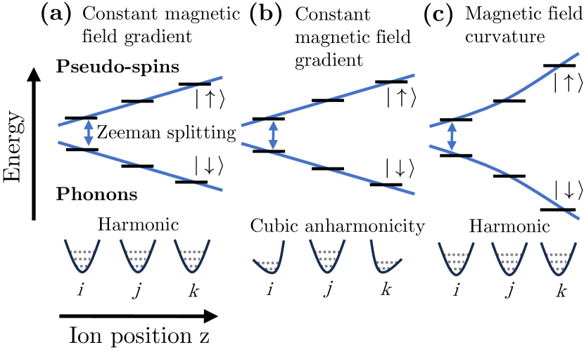
Figure 1: $\mathbf{(a)}$ The Magnetic Gradient Induced Coupling (MAGIC) scheme for trapped-ion quantum information processing employs a magnetic field gradient, which renders the resonance frequency of the internal pseudo-spin position-dependent. This couples the spin to the spatial phonon degree of freedom, which effectively generates a spin–spin coupling that can be used for entangling gates. In this work, we analyse higher-order contributions in such a setup, in particular $\mathbf{(b)}$ anharmonicities in the vibrational degrees of freedom due to Coulomb repulsion and $\mathbf{(c)}$ curvature of the magnetic field, which can lead to additional three-body and two-body interactions, local field corrections, as well as spin–phonon couplings.

In this work, we investigate the effects of higher-order contributions in the MAGIC setup. These include in particular residual terms coming from a third-order expansion of the Coulomb interactions (see also [23]), spatial dependence of the magnetic field, and anharmonicities of the individual trapping potentials. As we show, applying the canonical unitary transformation on the axial phonon modes that is used to derive the MAGIC scheme for trapped-ion logic [8, 9, 10], such higher-order terms induce three-qubit interactions as well as various types of terms that couple the pseudo-spins and the phonon vibrations. We show that in realistic situations the strength of most of these terms is negligible. Two contributions, however, can naturally achieve considerable strengths, especially when scaling to large ion chains. The first one takes the form of a phonon-occupation-dependent longitudinal field, whose strength increases with ion chain length and which for typical parameters can become comparable to the two-qubit interaction. Fortunately, such terms can be easily compensated by a detuning of the microwave frequency from the qubit resonance or suitable dynamical decoupling schemes [23]. The second type of contributions that needs care is a (well-known) two-to-one conversion between phonon modes [24]. These vanish if all phonon modes are ground-state cooled. As three-qubit interactions and spin–phonon couplings may be desired terms for various applications, ranging from quantum simulation [25, 26, 27, 28, 29] to quantum optimization [30, 31, 32], we also discuss possible strategies to engineer such terms. This work constitutes a systematic analysis of higher-order terms in the MAGIC setup, an important step for transitioning this type of quantum hardware from academic prototypes to mature technology.

This paper is structured as follows. In Sec. II, we review the MAGIC scheme for trapped-ion quantum information processing. In Sec. III, we compute the influence of terms due to various third-order expansions, including numerical estimates of their resulting strengths. These are a third-order expansion of the Coulomb repulsion between ions (Sec. III.2) and an external anharmonicity acting locally at each ion (Sec. III.3). Sec. IV is dedicated to the effects of an applied magnetic field with non-vanishing curvature. We compare the resulting strengths to different schemes known in the literature to generate such terms in Sec. V. Finally, Sec. VI contains our conclusions.

II Effective spin–spin interaction of trapped ions subject to a magnetic field gradient

The MAGIC scheme for quantum computation [8, 9, 10] uses microwaves instead of optical lasers to address ions and implement quantum gates. Since microwaves cannot be focused on individual ions, a magnetic field gradient is used to Zeeman-shift the resonance frequency of each ion and make them individually addressable in frequency space. Furthermore, the magnetic field gradient induces an Ising-type always-on all-to-all coupling between the ions, even in the absence of any driving fields, which can be used to synthesize quantum gates [33, 13] or perform adiabatic quantum sweeps [34]. Here, we give a concise review of the derivation of the spin–spin coupling. We refer to the literature for further details [8, 9, 10].

We consider a one-dimensional (1D) ion chain, elongated in the $z$ direction. The ions are subject to a static magnetic field with a constant gradient $\partial_{z}B$ in the axial direction $z$, $\bm{B}(z)=\bm{B}_{0}+\partial_{z}Bz\bm{\hat{e}}_{z}+\mathcal{O}(z^{2})$, where $\bm{B}_{0}$ is a constant offset field. In Appendix A, we generalize this setting to gradients in the transversal directions. Moreover, we will discuss the effect of a field with non-vanishing curvature in Sec. IV. We further assume that we use magnetically sensitive states as our qubit states (typically states from a hyperfine ground manifold with a resonance frequency in the microwave regime [35, 12, 14]) to make them individually addressable. The spatially varying magnetic field gives rise to a position-dependent resonance frequency $\omega(z)$, which in general has to be calculated numerically or can be estimated using the Breit–Rabi formula [36]. Under weak Zeeman splitting, which holds for the examples considered in this work, provided the offset field $\bm{B}_{0}$ is sufficiently small, the resonance frequency can be obtained as $\omega(z)=(g_{F}^{(e)}m_{F}^{(e)}-g_{F}^{(g)}m_{F}^{(g)})\mu_{\mathrm{B}}B(z)/\hbar$. Here, $g_{F}^{(g)}$ and $g_{F}^{(e)}$ are, respectively, the Landé $g$-factors of the qubit ground and excited state with total atomic angular momentum $F$, $m_{F}^{(g)}$ and $m_{F}^{(e)}$ are the corresponding magnetic quantum numbers, and $\mu_{\mathrm{B}}$ is the Bohr magneton. The internal energy of the ions is then given by

$$H_{\mathrm{int}}=\frac{\hbar}{2}\sum_{n=1}^{N}\omega(z_{n})\sigma_{z}^{(n)}\,,$$ (1)

where $\sigma_{z}^{(n)}$ denotes the Pauli-$Z$ operator acting on qubit $n$ at position $z_{n}$.

The resonance frequency can be expanded around the equilibrium position $z_{n,0}$ of ion $n$ as

$$\omega(z_{n})=\omega_{n}+\partial_{z}\omega_{n}(z_{n}-z_{n,0})+\mathcal{O}(z_{n}^{2})\,,$$ (2)

where $\omega_{n}=\omega(z_{n,0})$ is the resonance frequency and $\partial_{z}\omega_{n}=\partial\omega(z_{n,0})/\partial z$ the first derivative at the position of the ion. Higher-order terms in this expansion will be discussed in Sec. IV. Denoting the excursion of ion $n$ from its equilibrium position as $q_{n}=z_{n}-z_{n,0}$, we can then write the internal energy as

$$H_{\mathrm{int}}=-\frac{\hbar}{2}\sum_{n=1}^{N}\omega_{n}\sigma_{z}^{(n)}-\frac{\hbar}{2}\sum_{n=1}^{N}\partial_{z}\omega_{n}q_{n}\sigma_{z}^{(n)}.$$ (3)

Additionally, the ions have an energy associated with their external degrees of freedom, composed of their kinetic energy, the potential energy due to the trap, as well as their mutual Coulomb repulsion:

$$H_{\mathrm{ext}} =H_{\mathrm{kin}}+V(\bm{z})$$

$$=H_{\mathrm{kin}}+V_{\mathrm{trap}}(\bm{z})+V_{\mathrm{Coul}}(\bm{z})$$ (4)

$$=\frac{1}{2m}\sum_{n=1}^{N}p_{z,n}^{2}+\frac{m}{2}\omega_{z}^{2}\sum_{n=1}^{N}z_{n}^{2}+\frac{e^{2}}{8\pi\epsilon_{0}}\sum_{n\neq l}^{N}\frac{1}{|z_{n}-z_{l}|}\,.$$

Here, the vector $\bm{z}$ contains the positions of all ions, $e$ is the charge of the ions, $m$ their mass, $\epsilon_{0}$ the vacuum permittivity, and $p_{z,n}$ is the momentum of ion $n$ in the axial direction. For now, we will consider a harmonic trap with angular frequency $\omega_{z}$ and expand the potential energies around the ions’ equilibrium positions up to second order, yielding (after dropping a constant term)

$$H_{\mathrm{ext}}=\frac{1}{2m}\sum_{n=1}^{N}p_{z,n}^{2}+\frac{m}{2}\sum_{n=1}^{N}\sum_{l=1}^{N}A_{nl}q_{n}q_{l}+\mathcal{O}(q^{3})\,,$$ (5)

with $A_{nl}=\partial^{2}V(\bm{z}_{0})/\partial z_{n}\partial z_{l}$. In sections III.2 and III.3, we will discuss the effects of higher-order terms in the expansion of the potential energy.

The matrix $A$ is symmetric and real and can thus be diagonalized as $D=S^{-1}AS$ with an orthogonal matrix $S$. Since $A$ is a positive-definite Hessian (it results from an expansion around the minimum of the potential energy), its eigenvalues are positive and can be written as $\nu_{l}^{2}$. We can now express the local coordinates $q_{n}$ in terms of collective normal modes $Q_{l}$,

$$q_{n}=\sum_{l=1}^{N}S_{nl}Q_{l}\,.$$ (6)

These diagonalize the external Hamiltonian to

$$H_{\mathrm{ext}}=\frac{1}{2m}\sum_{n=1}^{N}P_{n}^{2}+\frac{m}{2}\sum_{n=1}^{N}\nu_{n}^{2}Q_{n}^{2}\,,$$ (7)

where we have defined $\bm{P}=S^{-1}\bm{p}_{z}$.

We can quantize the external Hamiltonian by introducing phonon creation and annihilation operators for the normal modes:

$$Q_{l}=\Delta z_{l}(a^{\dagger}_{l}+a_{l})\,,$$ (8)

with $\Delta z_{l}=\sqrt{\hbar/2m\nu_{l}}$ being the width of the ground-state wave packet of the quantum harmonic oscillator. The overall Hamiltonian $H=H_{\mathrm{int}}+H_{\mathrm{ext}}$ can now be expressed as

$$H= -\frac{\hbar}{2}\sum_{n=1}^{N}\omega_{n}\sigma_{z}^{(n)}-\frac{\hbar}{2}\sum_{n=1}^{N}\sum_{l=1}^{N}\partial_{z}\omega_{n}S_{nl}\Delta z_{l}(a^{\dagger}_{l}+a_{l})\sigma_{z}^{(n)}$$

$$+\hbar\sum_{n=1}^{N}\nu_{n}a^{\dagger}_{n}a_{n}\,.$$ (9)

We can decouple the internal and external degrees of freedom (spins and phonons) via a suitable unitary transformation [8, 10] (in some contexts known as polaron transformation [37]), $\tilde{H}=U^{\dagger}HU$, with

$$U =\exp\left(-\frac{i}{\hbar}\sum_{n=1}^{N}\sum_{l=1}^{N}\Delta z_{l}\epsilon_{nl}\sigma_{z}^{(n)}P_{l}\right)\,,$$ (10a)

$$\epsilon_{nl} =\frac{\Delta z_{l}\partial_{z}\omega_{n}}{\nu_{l}}S_{nl}\,.$$ (10b)

Here, we have defined the effective Lamb–Dicke parameter $\epsilon_{nl}$, describing how strongly ion $n$ (with internal transition frequency $\omega_{n}$) couples to phonon mode $l$ (with frequency $\nu_{l}$).

With the transformed phonon operators

$$\tilde{a}_{l}=U^{\dagger}a_{l}U=a_{l}+\frac{1}{2}\sum_{n}\epsilon_{nl}\sigma_{z}^{(n)}$$ (11)

(and unchanged spin operators $\tilde{\sigma}_{z}^{(n)}=\sigma_{z}^{(n)}$), the total Hamiltonian yields the desired two-body spin–spin interaction,

$$\tilde{H}^{(2)}= -\frac{\hbar}{2}\sum_{n=1}^{N}\omega_{n}\sigma_{z}^{(n)}+\hbar\sum_{n=1}^{N}\nu_{n}a^{\dagger}_{n}a_{n}$$

$$-\frac{\hbar}{2}\sum_{i<j}^{N}J_{ij}^{(2)}\sigma_{z}^{(i)}\sigma_{z}^{(j)}\,,$$ (12)

with the spin–spin coupling strength

$$J_{ij}^{(2)}=\sum_{n=1}^{N}\nu_{n}\epsilon_{in}\epsilon_{jn}\,.$$ (13)

This effective Hamiltonian is valid up to second order in the potential energy and linear order in the spatial dependence of magnetic field, owing to the Taylor expansions leading to the quadratic Hamiltonian in section II. Note that the polaron transformation from Eq. (II) to section II is exact in the sense that it does not involve any further approximations.

The spin–spin coupling strength $J_{ij}^{(2)}$ can be tuned via the magnetic field gradient and the strength of the external harmonic trap, since $J_{ij}^{(2)}\sim(\partial_{z}B/\nu)^{2}$. By employing different trapping potentials along the chain (not necessarily harmonic), coupling strengths between different pairs of ions can be enhanced or reduced [11]. Furthermore, by transferring state populations to magnetic insensitive states, specific ions can be completely excluded from the spin–spin interaction, permitting to engineer specific global gates [13].

Example: MAGIC with ^171_Yb+ ions

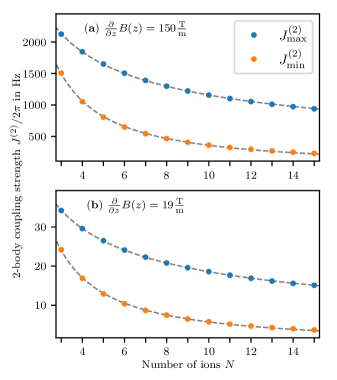
Figure 2: Spin–spin coupling strengths in the MAGIC scheme, calculated as a function of the number of ^171_Yb+ ions $N$ in a chain with trapping frequency $\omega_{z}=2\pi\times$130\text{\,}\mathrm{kHz}$$ and magnetic field gradient (a) $150\text{\,}\mathrm{T}\text{\,}{\mathrm{m}}^{-1}$ and (b) $19\text{\,}\mathrm{T}\text{\,}{\mathrm{m}}^{-1}$. Depicted are only the largest coupling strength $J^{(2)}_{\mathrm{max}}$ (blue), occurring between two neighboring ions at the edges of the chain, as well as the smallest coupling strength $J^{(2)}_{\mathrm{min}}$ (orange), felt by the most distant ions at opposite ends of the chain. The decrease of $J^{(2)}_{\mathrm{max}}$ follows the law $N^{-1/2}$ to good approximation, while $J^{(2)}_{\mathrm{min}}$ decreases approximately as $N^{-1.19}$. Corresponding fits are shown as grey dashed lines.

To illustrate realistically achievable spin–spin coupling strengths, we numerically calculate $J_{ij}^{(2)}$ for a chain of five ^171_Yb+ ions with trapping frequency $\omega_{z}=2\pi\times$130\text{\,}\mathrm{kHz}$$ and a magnetic field gradient of $\partial_{z}B=$19\text{\,}\mathrm{T}\text{\,}{\mathrm{m}}^{-1}$$, realized experimentally in Ref. [12]. We consider the states $\ket{F=0,m_{F}=0}$ and $\ket{F=1,m_{F}=+1}$ ($g_{F}\approx 1$) in the ground state hyperfine manifold as our qubit. The resonance frequency is then given by $\omega(z)\simeq-\mu_{\mathrm{B}}B(z)/\hbar$ [13]. The largest coupling strength occurs between the two outer neighboring ions at both edges of the chain: $J_{12}^{(2)}=J_{45}^{(2)}\approx 2\pi\times$26.5\text{\,}\mathrm{Hz}$$. The weakest coupling occurs between the leftmost and outermost ion: $J_{15}^{(2)}\approx 2\pi\times$12.9\text{\,}\mathrm{Hz}$$. For a stronger magnetic field gradient of $150\text{\,}\mathrm{T}\text{\,}{\mathrm{m}}^{-1}$, which is feasible with current technology [14, 38], the maximal (minimal) spin–spin coupling strength increases to $J_{12}^{(2)}=J_{45}^{(2)}\approx 2\pi\times$1650\text{\,}\mathrm{Hz}$$ ($J_{15}^{(2)}\approx 2\pi\times$805\text{\,}\mathrm{Hz}$$).

In Fig. 2, we plot the scaling behavior of the maximal and minimal coupling strengths for different numbers of ions in the chain, for the same trapping frequency and for the same two choices of magnetic field gradients as above. From a numerical fit (grey dashed lines), the maximal spin–spin coupling strength decreases as $N^{-0.51\pm 0.01}$ , matching the value $N^{-1/2}$ caused by the increasing inertia of larger ion crystals in the Cirac–Zoller gate [40] or the Mølmer–Sørensen gate [41].

In addition, we find the minimal spin–spin interaction diminishes as $N^{-1.19\pm 0.01}$. This stronger decrease can be attributed to the large distance between the involved ions (equivalent to $N$, the length of the ion chain) in interplay with contributions from phonons beyond the center-of-mass mode, which can lead to spatially decreasing interactions [42, 43, 44, 45, 46].

III Higher-order contributions from the potential energy

In the above, we have outlined the standard derivation of the effective spin–spin interaction arising in trapped-ion systems from the presence of a magnetic field gradient. This spin–spin interaction has been achieved by expanding the external potential governing the vibrational modes and the internal energy of the pseudo-spins to second order in the displacements from their equilibrium positions. In what follows, we investigate sources of higher-order terms in these expansions, which may contribute to the interactions in a MAGIC trapped-ion quantum computer.

This section is devoted to higher-order terms stemming from the potential energy associated with the external degrees of freedom of the ions.

We first derive the general form of the leading corrections to the Hamiltonian, giving rise to three-body spin–spin, spin–phonon, and phonon–phonon couplings (Sec. III.1). Subsequently, we address specifically the effects of cubic anharmonicities in the Coulomb repulsion (Sec. III.2) as well as in the external trapping potential (Sec. III.3). As we show by computing their natural strength using experimentally relevant parameters, they constitute negligible perturbations or can be compensated in typical setups, though in principle a device specifically designed to enhance these higher-order contributions might leverage them for quantum information processing tasks.

III.1 General third-order expansion of the potential

To start with, we calculate the effect of higher-order contributions of the external potential acting on the ion crystal. In this section, we focus on the Coulomb repulsion between ions. These contributions will naturally occur in any trapped-ion setup using a phonon bus, though we discuss their effect here specifically for the MAGIC platform. We start with general derivations, which we will adapt also in the next section for anharmonicities in the trapping potential, and then specialize to the Coulomb repulsion.

Extending the expansion of the potential energy $V$ of a 1D trapped-ion chain given in Eq. (II) up to third order, we obtain

$$\begin{split}V(\bm{z})&=V(\bm{z}_{0})+V^{(2)}(\bm{z})+V^{(3)}(\bm{z})+\mathcal{O}(\bm{z}^{4})\\ &=V(\bm{z}_{0})+\sum_{i,j}\frac{A_{ij}}{2}q_{i}q_{j}+\sum_{\mathclap{i,j,k}}\frac{B_{ijk}}{6}q_{i}q_{j}q_{k}+\mathcal{O}(q^{4})\,,\end{split}$$ (14)

with

$$A_{ij} =\left.\frac{\partial^{2}V}{\partial q_{i}\partial q_{j}}\right|_{\bm{z}_{0}},$$ (15)

$$B_{ijk} =\left.\frac{\partial^{3}V}{\partial q_{i}\partial q_{j}\partial q_{k}}\right|_{\bm{z}_{0}}.$$ (16)

The quadratic terms form the harmonic part of the potential [see eq. 7], whose eigenmodes will be used to express the higher-order terms. As in the previous section, the matrix $A$ is diagonalized by the normal modes $\bm{Q}$, which are related to the position operators via Eq. (6) and quantized through ladder operators via Eq. (8). The cubic terms $B_{ijk}$ can derive either solely from a higher-order expansion of the Coulomb potential, or additionally from anharmonicities in the trapping potential. These scenarios will be analyzed separately later. In principle, the above expansion can be continued to any desired higher order, but the resulting effects will be subleading (see also Ref. [23]).

We note that at this order of expansion of the external potential, the axial phonon modes couple to the transverse modes [24]. Here, we neglect this effect as we assume (i) axial and transverse modes to live at vastly different energy scales and (ii) the phonon modes to be ground-state cooled. We discuss the contributions from transverse modes in Appendix A.

Inserting the quantized normal modes, the anharmonic part of Eq. (14) reads

$$V^{(3)}=\frac{1}{6}\sum_{i,j,k}B_{ijk}\sum_{l,r,s}S_{il}S_{jr}S_{ks}\Delta z_{l}\Delta z_{r}\Delta z_{s}\\ \times(a_{l}^{\dagger}+a_{l})(a_{r}^{\dagger}+a_{r})(a_{s}^{\dagger}+a_{s})\,.$$ (17)

Adding this contribution to the Hamiltonian in Eq. (II) and applying the polaron transformation of Eq. (10) yields the total Hamiltonian $\tilde{H}=\tilde{H}^{(2)}+\tilde{H}^{(3)}$ of the system, given by

$$\tilde{H}=\tilde{H}^{(2)}+\frac{1}{6}\sum_{ijk}C_{ijk}\Big{(}a_{i}^{\dagger}+a_{i}+\sum_{n}\epsilon_{ni}\sigma_{z}^{(n)}\Big{)}\\ \times\Big{(}a_{j}^{\dagger}+a_{j}+\sum_{n}\epsilon_{nj}\sigma_{z}^{(n)}\Big{)}\Big{(}a_{k}^{\dagger}+a_{k}+\sum_{n}\epsilon_{nk}\sigma_{z}^{(n)}\Big{)}\,.$$ (18)

Here, $\tilde{H}^{(2)}$ is the standard MAGIC Hamiltonian in Eq. (II), resulting from an expansion of the potential up to second order, and we have defined

$$C_{ijk}=\sum_{mnl}B_{mnl}S_{mi}S_{nj}S_{lk}\Delta z_{i}\Delta z_{j}\Delta z_{k}\,.$$ (19)

Sorting the terms by their order of spin interactions, we get

$$\tilde{H} =\tilde{H}^{(2)}+\hbar\sum_{i<j<k}J_{ijk}^{(3)}\sigma_{z}^{(i)}\sigma_{z}^{(j)}\sigma_{z}^{(k)}$$

$$\hphantom{={}}+\frac{1}{2}\sum_{ijk}C_{ijk}\big{(}a_{i}^{\dagger}+a_{i}\big{)}\sum_{nm}\epsilon_{nj}\epsilon_{mk}\sigma_{z}^{(n)}\sigma_{z}^{(m)}$$

$$\hphantom{={}}+\frac{1}{2}\sum_{ijk}C_{ijk}\big{(}a_{i}^{\dagger}a_{j}^{\dagger}+a_{i}a_{j}+a_{i}^{\dagger}a_{j}+a_{i}a_{j}^{\dagger}\big{)}\sum_{n}\epsilon_{nk}\sigma_{z}^{(n)}$$

$$\hphantom{={}}+\frac{1}{6}\sum_{ijk}C_{ijk}\big{(}a_{i}^{\dagger}a_{j}^{\dagger}a_{k}^{\dagger}+a_{i}a_{j}a_{k}+a_{i}^{\dagger}a_{j}^{\dagger}a_{k}+a_{i}^{\dagger}a_{j}a_{k}^{\dagger}$$

$$\hphantom{=+\frac{1}{6}\sum_{ijk}C_{ijk}\big{(}}+a_{i}a_{j}^{\dagger}a_{k}^{\dagger}+a_{i}^{\dagger}a_{j}a_{k}+a_{i}a_{j}^{\dagger}a_{k}+a_{i}a_{j}a_{k}^{\dagger}\big{)}\,.$$ (20)

One of the corrections to the standard MAGIC Hamiltonian $\tilde{H}^{(2)}$ is a three-body spin interaction, given by

$$\tilde{H}^{(3)}=\hbar\sum_{i<j<k}J_{ijk}^{(3)}\sigma_{z}^{(i)}\sigma_{z}^{(j)}\sigma_{z}^{(k)}$$ (21)

with three-body interaction strength

$$\hbar J_{ijk}^{(3)} =\sum_{a,b,c,l,r,s}B_{abc}S_{al}S_{br}S_{cs}\Delta z_{l}\Delta z_{r}\Delta z_{s}\epsilon_{il}\epsilon_{jr}\epsilon_{ks}$$

$$=\sum_{lrs}C_{lrs}\epsilon_{il}\epsilon_{jr}\epsilon_{ks}$$

$$=\sum_{a,b,c}B_{abc}\frac{J_{ia}^{(2)}}{\partial_{z}\omega_{a}}\frac{J_{jb}^{(2)}}{\partial_{z}\omega_{b}}\frac{J_{kc}^{(2)}}{\partial_{z}\omega_{c}}\,.$$ (22)

In Eq. (21), we left out contributions to the local fields that arise for two coinciding indices. As we will see below, their strength, just like the three-body interaction, is negligible in realistic situations, but they could also be compensated easily by modifying the microwave detunings accordingly. The other terms [second to fifth row of Eq. (III.1)] describe a coupling of phonon modes to two-body spin interactions and local fields, as well as the usual anharmonic phonon term appearing due to anharmonicities of the external potential [24].

III.2 Higher-order effects from the Coulomb interaction

Up to here, the discussion applies to general anharmonicities in the external trapping potential. To obtain concrete order-of-magnitude estimates, we now specialize to the case of anharmonicities deriving solely from the Coulomb interactions, discussing each of the above additional contributions term by term. This complements the analysis of Ref. [23], where the phonon dependency was discussed within a mean field approximation assuming thermal phonon populations, with qualitatively similar conclusions.

The strength of the additional terms in Eq. (III.1) is determined by the cubic expansion coefficients $B_{ijk}$. From the Coulomb repulsion, they can be evaluated as [24]

$$B_{ijk}=\frac{-6m\omega_{z}^{2}}{l}\sum_{q\neq i}\frac{u_{i}-u_{q}}{|u_{i}-u_{q}|^{5}}\\ \times(\delta_{ij}-\delta_{qj})(\delta_{ik}-\delta_{qk})\,,$$ (23)

where $l$ is the characteristic length scale, defined via $l^{3}=e^{2}/(4\pi\epsilon_{0}m\omega_{z}^{2})$ [47]. We have further defined dimensionless equilibrium positions by $\bm{u}=\bm{z}_{0}/l$.

III.2.1 Three-body spin interactions

As a concrete example, we calculate the three-body interaction strength in a one-dimensional chain of five ^171_Yb+ ions in an axial harmonic trapping potential of strength $\omega_{z}=2\pi\times$130\text{\,}\mathrm{kHz}$$ and an applied magnetic gradient of $150\text{\,}\mathrm{T}\text{\,}{\mathrm{m}}^{-1}$. The numerical computation is based on a microscopic model of the ion chain, where we first find the ions’ equilibrium positions and then diagonalize the phonon eigenmodes, from which we can then derive all relevant energy scales. In this example, we find the highest three-body interaction strength to be $J_{145}^{(3)}\approx 2\pi\times$0.006\text{\,}\mathrm{Hz}$$ ($J_{125}^{(3)}\approx-2\pi\times$0.006\text{\,}\mathrm{Hz}$$). Compared to the smallest two-body interaction strength in the same system, $J_{15}^{(2)}\approx 2\pi\times$805\text{\,}\mathrm{Hz}$$, the three-body spin interactions introduced by anharmonicities in the Coulomb repulsion are negligible.

III.2.2 Phonon-dependent two-body spin interactions

The term in the second row of Eq. (III.1) gives corrections of the form $\sim(a_{i}^{\dagger}+a_{i})\sigma_{z}^{(n)}\sigma_{z}^{(m)}$ to the MAGIC two-body spin couplings. Their strength scales as $C_{ijk}\epsilon_{nj}\epsilon_{mk}$, and is thus one order in the Lamb–Dicke parameter $\epsilon$ stronger than $J_{ijk}^{(3)}$. Formally, they are of the same order in the Lamb–Dicke parameter as the two-body interaction $J_{ij}^{(2)}$. However, the terms $\sim(a_{i}^{\dagger}+a_{i})\sigma_{z}^{(n)}\sigma_{z}^{(m)}$ are suppressed by another factor $C_{ijk}$; even more, in contrast to $J_{ij}^{(2)}$, they do not preserve phonon number, and can thus safely be neglected within a rotating wave approximation: In the interaction picture given by the diagonal phonon Hamiltonian $\hbar\sum_{n}\nu_{n}a_{n}^{\dagger}a_{n}$, the creation and annihilation operators gain a time dependence $a_{i}^{\dagger}\to e^{i\nu_{i}t}a_{i}^{\dagger}$. They thus rotate on a time scale significantly faster than $C_{ijk}\epsilon_{nj}\epsilon_{mk}$. For instance, in the above example of a chain of five ^171_Yb+ ions, the strength of the terms in the second row of Eq. (III.1) is $|C_{ijk}\epsilon_{nj}\epsilon_{mk}|\lesssim${10}^{-1}\text{\,}\mathrm{Hz}$$. This value corresponds to interaction scales that are weaker than typical coherence times in trapped-ion hardware [48, 49]. Moreover, it is orders of magnitude smaller than even the smallest axial phonon frequency, $\omega_{\mathrm{COM}}=\omega_{z}=2\pi\times$130\text{\,}\mathrm{kHz}$$, such that this contribution can be neglected in a rotating wave approximation.

III.2.3 Spin-dependent phonon pair production and annihilation

The term in the third row of Eq. (III.1) has parts with different physical interpretation, which need to be discussed separately. In the same interaction picture as above, the terms creating (and annihilating) phonon pairs $a_{i}^{\dagger}a_{j}^{\dagger}$ (and $a_{i}a_{j}$) rotate with a frequency $\nu_{i}+\nu_{j}$, which is much larger than the associated energy scale $C_{ijk}\epsilon_{nk}$. Again, for the above example with five ions, we get corrections on the order of $|C_{ijk}\epsilon_{nk}|\lesssim$undef\text{\,}\mathrm{Hz}$$. As the phonon frequencies are orders of magnitude larger, these terms can again safely be neglected within a rotating wave approximation.

III.2.4 Spin-dependent phonon hopping

In contrast, the number-preserving terms of the form $a_{i}^{\dagger}a_{j}$ rotate with the frequency $\left|\nu_{i}-\nu_{j}\right|$. For axial phonons and small systems, the difference of phonon mode frequencies is large (e.g., for a chain of five ions in a trapping potential of $\omega_{z}=2\pi\times$130\text{\,}\mathrm{kHz}$$, phonon modes are separated by at least about $2\pi\times$80\text{\,}\mathrm{kHz}$$). Terms with $i\neq j$ thus still rotate rapidly as compared to the time scale $C_{ijk}\epsilon_{nk}$ and can be neglected.

III.2.5 Phonon-occupation-dependent longitudinal field

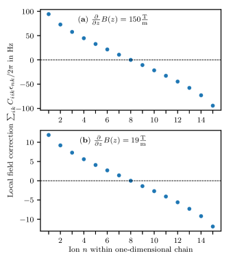
Figure 3: Corrections to the local field acting on each ion $n$ due to the anharmonicity of the Coulomb repulsion, $\sum_{ik}C_{iik}\epsilon_{nk}\sigma_{z}^{(n)}$ [third line in Eq. (III.1)]. Values computed for a chain of 15 ^171_Yb+ ions with a trapping frequency of $\omega_{z}=2\pi\times$130\text{\,}\mathrm{kHz}$$ and magnetic field gradients of (a) $150\text{\,}\mathrm{T}\text{\,}{\mathrm{m}}^{-1}$ and (b) $19\text{\,}\mathrm{T}\text{\,}{\mathrm{m}}^{-1}$, assuming ground-state-cooled phonons. These corrections are highly inhomogeneous and can acquire significant values comparable to spin–spin couplings (see Fig. 2).

We are thus left with terms where $i=j$, which give a correction to the local fields of strength $\sim\leavevmode\nobreak\ \sum_{ik}C_{iik}\epsilon_{nk}{(2n_{i}+1)}$, where $n_{i}=a_{i}^{\dagger}a_{i}$. Again, in the example of a chain of five ^171_Yb+ ions with $\omega_{z}=2\pi\times$130\text{\,}\mathrm{kHz}$$ and a magnetic gradient of $150\text{\,}\mathrm{T}\text{\,}{\mathrm{m}}^{-1}$, and assuming zero phonon number excitations ($n_{i}=0$), we get corrections on the order of ${10}^{1}\text{\,}\mathrm{kHz}$. There are largest for the outermost ions at the edges of the chain ($n=1$ and $n=5$), amounting to $\sum_{ik}C_{iik}\epsilon_{nk}\approx\pm 2\pi\times$49.2\text{\,}\mathrm{Hz}$$. For a magnetic gradient of $19\text{\,}\mathrm{T}\text{\,}{\mathrm{m}}^{-1}$, as is used in current experiments [12], this magnitude drops to $2\pi\times$6.2\text{\,}\mathrm{Hz}$$. While this is smaller than the coupling strengths $J^{(2)}/2\pi\approx$13\text{\,}\mathrm{Hz}27\text{\,}\mathrm{Hz}$$, it may generate a small parasitic contribution to the two-qubit gates (see Ref. [23] for a discussion of the magnitude of these gate errors).

In Fig. 3, we show the behavior of these local field corrections across a chain of 15 ions for magnetic field gradients of (a) $150\text{\,}\mathrm{T}\text{\,}{\mathrm{m}}^{-1}$ and (b) $19\text{\,}\mathrm{T}\text{\,}{\mathrm{m}}^{-1}$. The corrections are largest towards the edges of the chain (equal magnitudes with opposite signs) and vanish for the ion at the center. The magnitude of the correction scales approximately linearly with the distance to the center of the chain, with larger deviations toward the edges. When plotted not against ion number but actual ion position in the chain, the curve straightens out somewhat, though it still does not behave perfectly linearly. Comparing the largest corrections at the edges of the chain ($\approx 2\pi\times$11.9\text{\,}\mathrm{Hz}$$) to the spin–spin coupling strengths shown in Fig. 2 ($J_{\mathrm{max}}^{(2)}/2\pi\approx$15.1\text{\,}\mathrm{Hz}$$), we find them to be already of the same order of magnitude as the always-on spin–spin couplings for this system size.

In Fig. 4, we plot the scaling of these largest corrections at the edges of the chain with system size, again for the same values of the magnetic field gradient. We find that the local field corrections increase with the length of the chain. In contrast, as illustrated above in Fig. 2, the spin–spin coupling strengths decrease. Thus, these local corrections become more relevant as the system size increases. Phenomenologically, we find the scaling behaviour to be best described by a power law with logarithmic corrections of the form $N^{a}\log(bN)$, with fitting parameters $a=0.18\pm 0.01$, $b=1.38\pm 0.04$ for $150\text{\,}\mathrm{T}\text{\,}{\mathrm{m}}^{-1}$ and $a=0.18\pm 0.01$, $b=1.35\pm 0.07$ for $19\text{\,}\mathrm{T}\text{\,}{\mathrm{m}}^{-1}$.

The presence of a parasitic local field could constitute an issue for the precise functioning of the two-qubit gate or for the correct definition of cost functions in quantum optimization [50]. Fortunately, since the associated terms are proportional to $\sigma_{z}^{(n)}$, even for nonzero (but fixed) phonon excitation numbers they can be offset be adjusting the microwave detunings from the qubit resonances, which result in local fields $\sim(\omega_{n}^{(\mathrm{MW})}-\omega_{n})\sigma^{(n)}_{z}$. In typical trapped-ion devices, such a compensation is often routine, even for terms many orders of magnitude stronger than in this case. For instance, in a Mølmer–Sørensen setup on the axial modes of ^40_Ca+ ions, undesired off-resonant excitation of dipole transitions can induce inhomogeneous light shifts on the order of $2\text{\,}\mathrm{kHz}3\text{\,}\mathrm{kHz}$, which need to be calibrated and compensated [43]. In addition, already simple dynamical-decoupling techniques can remove undesired terms $\sim\sigma_{z}^{i}$ [51, 23].

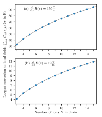
Figure 4: Scaling of the largest correction $\sum_{ik}C_{iik}\epsilon_{1k}\sigma_{z}^{(1)}$ (on the leftmost edge) to the local fields with increasing number of ^171_Yb+ ions in the chain. Calculations were done for a vanishing phonon occupation, a trapping frequency of $\omega_{z}=2\pi\times$130\text{\,}\mathrm{kHz}$$, and magnetic gradients of (a) $150\text{\,}\frac{\mathrm{T}}{\mathrm{m}}$ and (b) $19\text{\,}\frac{\mathrm{T}}{\mathrm{m}}$. The absolute strength increases with chain length, rendering this correction significant in particular when scaling to larger ion chains. Numerical fits (grey dashed lines) show a scaling $\propto N^{0.18}\log(1.38N)$.

III.2.6 Phonon creation, annihilation, and conversion terms

Finally, the two last lines of Eq. (III.1) contain terms that describe the generation/annihilation of triples of phonons as well as two-to-one phonon conversion, which have been discussed before [24]. The former terms can be neglected since they rotate with at least three times the trap frequency, which is much larger than the interaction strength $C_{ijk}$. The two-to-one conversion terms, however, require careful attention. As long as all modes are ground-state cooled, these terms vanish. They can also be suppressed by designing the trap parameters such that the phonon frequencies do not conspire to render such terms resonant. For the above setup with five ions and a magnetic field gradient of $150\text{\,}\mathrm{T}\text{\,}{\mathrm{m}}^{-1}$, the smallest frequency difference $\left|\nu_{i}+\nu_{j}-\nu_{k}\right|$ is about $27\text{\,}\mathrm{kHz}$. In this specific case, these terms can thus safely be neglected even if the chain is not fully cooled into the motional ground state. Nevertheless, these caveats need to be kept in mind especially when scaling up to large ion chains, where ground-state cooling becomes more challenging and resonances can appear more easily.

To summarize this part, among the various corrections to the MAGIC trapped-ion scheme that derive from a third-order expansion of the Coulomb repulsion, only phonon-number-dependent longitudinal fields as well as two-to-one phonon conversions can become sizable. The former can be compensated by microwave detunings, while the latter can be avoided by ground-state cooling of the phonon modes.

III.3 Cubic anharmonicities of the external trapping potential

In addition to the intrinsic anharmonicities given by the Coulomb potential, there could also be anharmonicities stemming from the external trapping potential. While such effects are often undesired for pristine quantum logic, anharmonicities can nowadays also be designed and exploited in a controlled way [52, 53]. Such anharmonic potentials can change the equilibrium positions of the ions and therefore modify the two-body interactions induced by a magnetic field gradient. This effect has been investigated in Ref. [11]. Here, we discuss the role of higher-order terms generated by anharmonicities in the external potential.

To this end, we consider a cubic contribution to the potential energy of the form

$$V^{(3)}(\bm{z}) =\sum_{n}\frac{\alpha_{n}}{6}(z_{n}-z_{n,0})^{3}\,,$$ (24)

where $\alpha_{n}$ describes the strength of the cubic anharmonicity felt by ion $n$. Such terms in the potential energy generate additional three-body spin–spin, spin–phonon, and phonon–phonon interactions, for which the general considerations discussed in Sec. III.2 apply. Here, we investigate the resulting three-body spin interaction in more detail.

Inserting the expansion coefficients $B_{ijk}=\delta_{ij}\delta_{jk}{\alpha_{i}}$ into section III.1, the three-spin coupling coefficients specialize to

$$\hbar J_{ijk}^{(3)}=\sum_{n}\frac{\alpha_{n}}{(\partial_{z}\omega_{n})^{3}}J_{in}^{(2)}J_{jn}^{(2)}J_{kn}^{(2)}\,.$$ (25)

In order to obtain a simple order-of-magnitude estimate for their typical strength, we first estimate the typical strength of the two-body spin interaction in eq. 13. For this purpose, we consider only the contribution from the center-of-mass (cm) mode, whose frequency coincides with the trap frequency, $\nu_{\mathrm{cm}}=\omega_{z}$, and whose matrix elements $S_{i,\mathrm{cm}}$ are given by $1/\sqrt{N}$. Assuming that the gradient of the resonance frequency is the same for all ions ($\partial_{z}\omega_{i}=\partial_{z}\omega$), we have $J^{(2)}\simeq\omega_{z}\epsilon^{2}$ with the effective Lamb–Dicke parameter $\epsilon=\partial_{z}\omega\Delta z/\omega_{z}\sqrt{N}$ and oscillator length $\Delta z=\sqrt{\hbar/2m\omega_{z}}$. Combining this expression with eq. 25, we can estimate the typical strength of the three-body coupling as

$$\hbar J^{(3)}\simeq\frac{1}{\sqrt{N}}\frac{\alpha\Delta z^{3}}{\hbar\omega_{z}}\mathinner{\epsilon}\hbar J^{(2)}=\frac{1}{\sqrt{N}}\alpha\Delta z^{3}\epsilon^{3}\,,$$ (26)

where we have made the additional simplifying assumption that the anharmonicity is the same at each ion position ($\alpha_{n}=\alpha$).

One may be tempted to engineer cubic terms in the potential similar to eq. 24 with the goal of harnessing the resulting three-body spin interaction for quantum information processing tasks. Unfortunately, as we argue in what follows, this endeavor is unlikely to be advantageous in practice.

To this end, we note that cubic contributions to the potential energy may severely affect the stability of the trap. For instance, an external potential of the form $V_{\mathrm{trap}}(\bm{z})=\sum_{n}m\omega_{z}^{2}z_{n}^{2}/2+\sum_{n}\alpha z_{n}^{3}/6$ with global anharmonicity $\alpha$ gives rise to terms as in eq. 24 with $\alpha_{n}=\alpha$. However, such a potential also shifts the equilibrium positions of the ions. Thus, in order to prevent ions from being ejected from the trap, the anharmonicity should be a somewhat small perturbation on top of the harmonic part, such that the potential still features a local minimum that is sufficiently deep and wide to trap the ions. That is, the energy scale $\alpha\Delta z^{3}$ should be well below the harmonic trapping energy $\hbar\omega_{z}$, requiring $\alpha\Delta z^{3}/\hbar\omega_{z}\ll 1$. On the other hand, the three-body interaction should be sufficiently strong in order to be of practical use. For example, a native three-qubit gate should outperform the equivalent gate synthesized from a combination of two-qubit gates. Thus, it is desirable that $J^{(3)}=\lambda J^{(2)}$ with $\lambda$ as large as possible (though typically well below unity). The estimate in eq. 26 can then be expressed as $\alpha\Delta z^{3}/\hbar\omega_{z}=\lambda\sqrt{N}/\epsilon$. As noted before, stability of the trapping potential requires this quantity to be sufficiently small, enforcing the hierarchy $\lambda=J^{(3)}/J^{(2)}\ll\epsilon/\sqrt{N}$. This means that the three-qubit interaction is bound to be weaker than the two-qubit interaction by a factor well below $\epsilon/\sqrt{N}$, which in realistic setups amounts to a suppression by at least one, if not several, orders of magnitude.

To circumvent the stability issues described above, one may attempt to engineer the terms in eq. 24 locally, i.e., without affecting the equilibrium positions of the ions, as may be possible, e.g., in segmented ion traps [52]. However, from a practical point of view, the electrodes creating such local potentials cannot be placed arbitrarily close to the ions, but require a certain minimum distance, which is typically large compared to the spacing between ions [52]. Consequently, it becomes difficult to create localized features varying on the scale of the oscillator length $\Delta z$, which is much smaller than the distance between ions. For example, it appears challenging to engineer localized external potentials stronger than the intrinsic Coulomb potential created by the ions themselves. Even if the strength of the local cubic potential was comparable to the characteristic energy scale of the anharmonic part of the Coulomb repulsion in eq. 23, $\alpha\Delta z^{3}=6m\omega_{z}^{2}\Delta z^{3}/l\approx$0.004$\,\hbar\omega_{z}$, the maximum three-body coupling strength would amount to only $J_{\mathrm{max}}^{(3)}/2\pi\approx$0.3\text{\,}\mathrm{Hz}$$ in a chain of $N=5$ ions with trapping frequency $\omega_{z}/2\pi=$130\text{\,}\mathrm{kHz}$$ and magnetic field gradient $\partial_{z}B=$150\text{\,}\mathrm{T}\text{\,}{\mathrm{m}}^{-1}$$, which is too low for typical applications. For comparison, a potential with a global cubic anharmonicity of the same strength would induce equally weak three-body interactions, but would not be able to trap the ions for the above parameters in its local minimum.

To sum up, while cubic anharmonicities can in principle be a route to engineering three-body interactions in the MAGIC setup, the comparatively slow three-qubit interaction rate and the substantial experimental overhead of realizing the required cubic anharmonicities in a stable way limit the practical use of this scheme. After all, our discussion reveals that moderate cubic anharmonicities typically have a negligible parasitic impact on the standard MAGIC setup.

IV Higher-order contributions from the magnetic field curvature

While anharmonicities in the external potential of the ion crystal appear in any trapped-ion platform, a higher-order contribution specific to the MAGIC setup originates from higher-order spatial derivatives of the magnetic field. To evaluate their effect, we expand the magnetic-field-dependent resonance frequency of the ions [see Eq. (2)] up to second order,

$$\begin{split}\omega(z_{n})&=\omega_{n}+\partial_{z}\omega(z_{n})\Big{\rvert}_{z_{n,0}}(z_{n}-z_{n,0})\\ &\hphantom{={}}+\frac{1}{2}\partial^{2}_{z}\omega(z_{n})\Big{\rvert}_{z_{n,0}}(z_{n}-z_{n,0})^{2}+\mathcal{O}\left(z_{n}^{3}\right)\,.\end{split}$$ (27)

The Hamiltonian $H_{\mathrm{int}}$ in Eq. (3), describing the internal energy of the ion chain, then becomes

$$H_{\mathrm{int}}=-\frac{\hbar}{2}\sum_{n}\Big{(}\omega_{n}+\partial_{z}\omega_{n}q_{n}+\frac{1}{2}\partial^{2}_{z}\omega_{n}q_{n}^{2}\Big{)}\sigma_{z}^{(n)}\,.$$ (28)

Inserting again the quantized normal modes, the internal energy Hamiltonian reads

$$H_{\mathrm{int}}=-\frac{\hbar}{2}\sum_{n}\omega_{n}\sigma^{(n)}-\frac{\hbar}{2}\sum_{nl}\partial_{z}\omega_{n}S_{nl}\Delta z_{l}\big{(}a_{l}^{\dagger}+a_{l}\big{)}\sigma_{z}^{(n)}\\ -\frac{\hbar}{4}\sum_{nlr}\partial^{2}_{z}\omega_{n}S_{nl}S_{nr}\Delta z_{l}\Delta z_{r}\big{(}a_{l}^{\dagger}+a_{l}\big{)}\big{(}a_{r}^{\dagger}+a_{r}\big{)}\sigma_{z}^{(n)}\,.$$ (29)

Performing, as before, the polaron transformation to decouple phonons and spins in the first order terms, Eq. (10), we obtain the total Hamiltonian $\tilde{H}=\tilde{H}^{(2)}+\tilde{H}^{(3)}$ with

$$\begin{split}\tilde{H}^{(3)}&=-\frac{\hbar}{4}\sum_{nlr}\partial_{z}^{2}\omega_{n}S_{nl}S_{nr}\Delta z_{l}\Delta z_{r}\sigma_{z}^{(n)}\\ &\times\Big{(}a_{l}^{\dagger}+a_{l}+\sum_{i}\epsilon_{il}\sigma_{z}^{(i)}\Big{)}\Big{(}a_{r}^{\dagger}+a_{r}+\sum_{j}\epsilon_{jr}\sigma_{z}^{(j)}\Big{)}\,.\end{split}$$ (30)

Again, $\tilde{H}^{(2)}$ is the standard MAGIC Hamiltonian, while $\tilde{H}^{(3)}$ are the corrections due to the expansion of the magnetic field distribution up to third order. We can sort all terms by their power in the spin operators and write

$$\begin{split}\tilde{H}&=\tilde{H}^{(2)}-\frac{\hbar}{4}\sum_{ijk}J_{ijk}^{(3)}\sigma_{z}^{(i)}\sigma_{z}^{(j)}\sigma_{z}^{(k)}\\ &\hphantom{={}}-\frac{\hbar}{2}\sum_{ijlr}\tilde{C}_{ilr}\epsilon_{jr}\big{(}a_{l}^{\dagger}+a_{l}\big{)}\sigma_{z}^{(i)}\sigma_{z}^{(j)}\\ &\hphantom{={}}-\frac{\hbar}{4}\sum_{ilr}\tilde{C}_{ilr}\big{(}a_{l}^{\dagger}a_{r}^{\dagger}+a_{l}^{\dagger}a_{r}+a_{l}a_{r}^{\dagger}+a_{l}a_{r}\big{)}\sigma_{z}^{(i)}\,,\end{split}$$ (31)

where we defined

$$\tilde{C}_{ilr}=\partial_{z}^{2}\omega_{i}S_{il}S_{ir}\Delta z_{l}\Delta z_{r}\,.$$ (32)

Analogously to the discussion of Sec. III.2, the terms in the second row give corrections to the two-body spin interactions of the form $(a_{l}^{\dagger}+a_{l})\sigma_{z}^{(i)}\sigma_{z}^{(j)}$. Again, these do not preserve phonon numbers and can be neglected within a rotating wave approximation. The terms in the third row only give corrections to local fields of strength $\sim\tilde{C}_{irr}(2n_{r}+1)$ with $n_{r}=a_{r}^{\dagger}a_{r}$ (neglecting phonon-number-non-preserving terms as before), which can be offset by microwave detunings or neglected for small magnetic field curvatures ($\tilde{C}_{irr}\propto\partial_{z}^{2}\omega_{i}$). Due to the different origin of the higher-order terms as compared to Sec. III.2, there are no cubic phonon terms in this expansion.

The remaining effective three-spin interaction is

$$\tilde{H}^{(3)} =-\frac{\hbar}{4}\sum_{ijk}J_{ijk}^{(3)}\sigma_{z}^{(i)}\sigma_{z}^{(j)}\sigma_{z}^{(k)}$$ (33)

with the three-body coupling strength

$$J_{ijk}^{(3)} =\sum_{lr}\partial^{2}_{z}\omega_{i}S_{il}S_{ir}\Delta z_{l}\Delta z_{r}\sum_{jk}\epsilon_{jl}\epsilon_{kr}\,.$$ (34)

The form of this term differs from the ones in the previous section [Eqs. (III.1) and (25)], since it did not derive from a contribution $\propto x^{3}$, but rather $\propto x^{2}\sigma^{z}$.

By defining $\gamma_{n}=\partial^{2}_{z}\omega_{n}/(\partial_{z}\omega_{n})^{2}$, i.e., the ratio between the magnetic field curvature and the square of the gradient, and using the spin–spin coupling strength given in Eq. (13), one can write this interaction even more compactly as

$$J_{nij}^{(3)}=\gamma_{n}J_{ni}^{(2)}J_{nj}^{(2)}\,.$$ (35)

Notably, $J_{nij}^{(3)}=J_{nji}^{(3)}$, but in general $J_{nji}^{(3)}\neq J_{jni}^{(3)}$. One can symmetrize the 3-body coupling strength to

$$\tilde{J}_{ijk}^{(3)} =\gamma_{i}J_{ij}^{(2)}J_{ik}^{(2)}+\gamma_{j}J_{ji}^{(2)}J_{jk}^{(2)}+\gamma_{k}J_{ki}^{(2)}J_{kj}^{(2)}\,,$$ (36)

which assumes a form similar to that obtained in Ref. [54] for a trapped-ion system driven close to the second sideband.

In analogy to the procedure for anharmonic external potentials in Sec. III.3, the typical strength of the three-body coupling induced by the magnetic field curvature can be estimated as

$$J^{(3)}=\frac{1}{\sqrt{N}}\frac{\partial_{z}^{2}\omega\Delta z}{\partial_{z}\omega}\mathinner{\epsilon}J^{(2)}=\frac{1}{N}\partial_{z}^{2}\omega\Delta z^{2}\epsilon^{2}\,.$$ (37)

Remarkably, this quantity scales quadratically with the effective Lamb–Dicke parameter $\epsilon$ and thus with the magnetic field gradient, like the two-body coupling $J^{(2)}$.

For a potential application of this “magnetic curvature induced three-body coupling” in quantum information processing, the quadratic variation of the local resonance frequency $\partial_{z}^{2}\omega$ over length scales on the order $\Delta z$ should be sufficiently large. However, similarly as for the local cubic potentials discussed in section III.3, in practice it is very hard to engineer magnetic field distributions with sufficiently sharp localized features.

Instead, we consider in what follows a global magnetic field curvature of the form $\bm{B}(z)=\bm{B}_{0}+(\mathinner{\partial_{z}B}z+\mathinner{\partial_{z}^{2}B}z^{2}/2)\bm{\hat{e}}_{z}+\mathcal{O}(z^{3})$. Unlike higher-order terms in the external potential, higher-order contributions to the magnetic field do not alter the equilibrium positions of the ions as they act on the internal degrees of freedom, but they can lead to a position-dependent magnetic-field gradient $\partial_{z}B(z_{n})$. As an example, we consider a magnetic field curvature of $\partial^{2}_{z}B\simeq${10}^{3}\text{\,}\mathrm{T}\text{\,}{\mathrm{m}}^{-2}$$, which can be reached using suitably designed Halbach magnets [55]. If the ion chain is centered around the origin, the variation of the magnetic field gradient is negligible, $\partial B(z_{n})/\partial z=\partial_{z}B+z_{n}\partial_{z}^{2}B\approx\partial_{z}B$, since the spacing between ions is on the order of $10\text{\,}\mathrm{\SIUnitSymbolMicro m}$. In addition, for five^171_Yb+ ions with a magnetic field gradient of $\partial_{z}B=$150\text{\,}\mathrm{T}\text{\,}{\mathrm{m}}^{-1}$$ and a trap frequency of $\omega_{z}/2\pi=$130\text{\,}\mathrm{kHz}$$, we obtain three-body coupling strengths of only $J^{(3)}\sim 2\pi\times${10}^{-5}\text{\,}\mathrm{Hz}$$, which is orders of magnitude too low for practical use. Nonetheless, this example underlines that, as long as the magnetic field gradient does not significantly vary on length scales comparable to the oscillator length $\Delta z$, parasitic effects from nonlinear gradients can safely be neglected in the standard MAGIC scheme.

V Comparison to existing schemes for generating higher-order interactions in trapped ions

As we have seen in the above, higher-order terms in the MAGIC setup naturally lead to three-body interactions and spin–phonon couplings. Since such types of interactions are key ingredients in applications ranging from quantum simulation of topological and Peierls phase transitions [26, 27] and lattice gauge theories [25, 28, 29] to improved schemes of quantum annealing [32, 30], one may wonder if there are feasible ways to engineer such interactions.

Indeed, various proposals have been designed for this purpose specifically with trapped-ion setups in mind. One rather generally applicable approach relies on obtaining three-body interactions perturbatively from two-body terms, e.g., via an energy penalty [56] or via a high-frequency expansion based on Floquet engineering [57]. The resulting three-body interactions can be as large as $2\pi\times$0.2\text{\,}\mathrm{kHz}$$ [56]. As a feature of the approach in Ref. [56], in the effective Hamiltonian the two-body interactions play no role any more.

Other approaches are based on continuously and simultaneously addressing the first and second sideband [54, 28], which results in the simultaneous presence of terms that are formally similar to the terms $q_{n}\sigma_{z}^{(n)}$ and $q_{n}^{2}\sigma_{z}^{(n)}$ that appear in Eq. (28). In this approach, the ability to use large Rabi frequencies on the first and second sideband can permit to reach three-body interactions as strong as $\sim 2\pi\times$1.6\text{\,}\mathrm{kHz}$$ [54]. A further promising proposal has recently been put forward based on a combination of discrete, spin-dependent displacement and squeezing pulses [58]. In a chain of four ^171_Yb+ ions, the authors estimate the gate time of a fully entangling three-qubit gate, $U=\exp\big{(}-\frac{\pi}{4}\sigma_{z}^{(i)}\sigma_{z}^{(j)}\sigma_{z}^{(k)}\big{)}$, to be $T\approx$130\text{\,}\mathrm{\SIUnitSymbolMicro s}$$ for feasible setups with laser-based control, corresponding to a three-body coupling strength on the order of $2\pi\times$1\text{\,}\mathrm{kHz}$$.

Finally, a standard way that is always possible given a universal gate set is to engineer the unitary three-qubit interactions through a combination of two-qubit and single-qubit gates. For example, a term of the form $\sigma_{z}^{(i)}\sigma_{z}^{(j)}\sigma_{z}^{(n)}$ can be realized using four Mølmer–Sørensen gates, see, e.g., Ref. [32]. Neglecting the gate time of single-qubit operations, one can associate an effective three-body strength to this gate sequence of order $J^{(3)}=J^{(2)}/4$, which is a rather sizable interaction strength. As in this case the unitary three-body gate is generated exactly, there are no additional two-body interactions.

We have also seen that the higher-order corrections can generate terms of the form $a_{i}a_{j}\sigma_{z}^{(n)}$ or $a_{i}\sigma_{z}^{(n)}\sigma_{z}^{(m)}$. In Ref. [25], it has been shown how these terms can be used to quantum simulate a lattice version of quantum electrodynamics. In that work, it was found that near-resonant addressing of first and second sidebands may generate interaction strengths up to $2\pi\times$120\text{\,}\mathrm{Hz}$$.

VI Conclusions

To summarize, in this article we have presented a thorough analysis of how higher-order terms in the external potential and the magnetic field take effect in the MAGIC scheme. We have derived the effective interactions that result on top of the desired two-body interactions after a polaron transformation on the axial phonon modes. There are two generic main contributions: phonon–spin couplings and three-body spin–spin interaction terms. As we have shown through our analysis, in typical situations such higher-order terms can safely be neglected as compared to the two-body interactions, and in particular also as compared to other error sources such as deriving from fluctuations or drifts in trap frequency, microwave or laser intensity, timing precisions, heating of phonon modes, spontaneous emission, etc [59]. Since such interaction terms may also be desired for certain applications, e.g., quantum simulation of strongly-correlated systems or enhanced quantum-optimization schemes, we have put these values in context by giving a brief survey on existing schemes to generate exploitable three-body interactions.

In contrast, there recently has been a proposal to utilize existing anharmonicities in the Coulomb repulsion (or explicitly engineer such anharmonicities) in order to generate noise-resilient entangling gates for trapped ions [60]. In such cases, the subleading interaction terms are unwanted error sources, whose magnitudes need to be carefully considered.

From our analysis, we have seen that anharmonicities in the potential energy can induce two types of terms that need some careful attention. The first one is a phonon-induced shift of the qubit resonance frequency—an effect that in the literature has been rarely discussed [23]. Its strength increases with chain length. Fortunately, it can be compensated by appropriate detuning of the microwave radiation. The second effect that requires attention is a two-to-one conversion of phonons [24]. It vanishes if all phonon modes are ground-state cooled, and it can be neglected in a rotating wave approximation if the trap is designed such that resonances between phonon frequencies are avoided. These potential effects need to be kept in mind in particular when scaling to large ion chains.

Our analysis provides a guideline for the precision necessary in engineering trapped-ion quantum hardware. Future work along this direction may include more detailed investigations of the radial modes (see App. A), which can become coupled to the axial modes by anharmonic potentials, as well as expansions to even higher order (e.g., fourth-order correction to the Coulomb potential). Similar analyses may also be important for other approaches, e.g., those based on Mølmer–Sørensen-type gates using laser beams [61, 62] or oscillating magnetic fields [63, 64, 65, 66]. Finally, our study may also inspire novel ways to exploit higher-order effects for the design of new quantum gates.

Appendix A Higher-order corrections from transversal phonon modes

In this appendix, we briefly discuss the corrections due to transversal phonon modes in an expansion of the potential energy up to third order. Although the transversal modes also cause corrections in a third-order expansion of the resonance frequencies of the ions, the corresponding terms are proportional to the curvature of the magnetic field in axial and radial directions. As argued in Sec. IV, such contributions can safely be neglected for realistic magnetic fields. We therefore focus here only on anharmonicities arising from the Coulomb potential.

For a one-dimensional ion chain in a harmonic trap, analogously to the discussion in Sec. III.2, the external potential can be expanded around the equilibrium position $\bm{q}_{0}$ as [24]

$$V(\mathbf{q}) =V(\bm{q}_{0})+V^{(2)}(\bm{q})+V^{(3)}(\bm{q})+\mathcal{O}(\bm{q}^{4})$$

$$=V(\bm{q}_{0})+\frac{1}{2}\sum_{\alpha=1}^{3}\sum_{i,j}A^{\alpha}_{ij}q_{i}^{(\alpha)}q_{j}^{(\alpha)}$$

$$\hphantom{={}}+\sum_{i,j,k}\tilde{B}_{ijk}q_{k}^{(3)}\left(2q_{i}^{(3)}q_{j}^{(3)}-3q_{i}^{(2)}q_{j}^{(2)}-3q_{i}^{(1)}q_{j}^{(1)}\right)$$

$$\hphantom{={}}+\mathcal{O}(\bm{q}^{4})\,,$$ (38)

where $q_{i}^{(3)}$ ($q_{i}^{(2)}$, $q_{i}^{(1)}$) is the displacement of ion $i$ from its equilibrium position in the axial (transversal) direction. Further, we have defined

$$A^{\alpha}_{ij} =\left.\frac{\partial^{2}V}{\partial q_{i}^{(\alpha)}\partial q_{j}^{(\alpha)}}\right|_{\bm{q}_{0}}\,,$$ (39)

$$\tilde{B}_{ijk} =\frac{m\omega_{z}^{2}}{2l}\sum_{q\neq i}\frac{\text{sgn}(u_{q}-u_{i})(\delta_{ij}-\delta_{qj})(\delta_{ik}-\delta_{qk})}{(u_{q}-u_{i})^{4}}\,,$$ (40)

with the ion mass $m$, the axial trap frequency $\omega_{z}$, the characteristic length scale $l$ (defined as $l^{3}=e^{2}/4\pi\epsilon_{0}m\omega_{z}^{2}$), and the dimensionless equilibrium positions $\bm{u}=\bm{q}_{0}/l$.

The second-order terms in Eq. (A) are decoupled. After quantizing and performing a polaron transformation on these terms with respect to all axial and transversal modes, similarly as in Sec. II, we arrive again at Eq. (II), where the spin–spin coupling strength is now given by

$$J_{ij}^{(2)} =\sum_{\alpha=1}^{3}\sum_{n=1}^{N}\nu_{n}^{(\alpha)}\epsilon^{(\alpha)}_{in}\epsilon^{(\alpha)}_{jn}\,.$$ (41)

Here, we have defined the $n$-th phonon mode frequency $\nu_{n}^{(\alpha)}$ in direction $\alpha=1,2,3$ and the effective Lamb–Dicke parameter $\epsilon^{(\alpha)}_{in}$ describing the coupling of ion $i$ to said mode, cf. Eq. (10b). The coupling strength scales as $J_{ij}^{(2)}\sim\sum_{\alpha}(\partial_{\alpha}B/\nu^{(\alpha)})^{2}$, where $\partial_{\alpha}B$ is the magnetic field gradient in direction $\alpha$. If the magnetic gradient vanishes in both transversal directions, the spin–spin coupling strength reduces to Eq. (13) stated in the main text.

For the third order terms in Eq. (A) (third row), we find one term with only axial motion ($\sim q_{k}^{(3)}q_{i}^{(3)}q_{j}^{(3)}$), which we have already discussed in Sec. III.2, and two terms which couple axial and transversal motion ($\sim q_{k}^{(3)}q_{i}^{(2)}q_{j}^{(2)}$ and $\sim q_{k}^{(3)}q_{i}^{(1)}q_{j}^{(1)}$). For the latter two terms, we can perform the same analysis as for the first term (see Sec. III.2).

If the magnetic gradient vanishes in the transversal directions, we are then left with two terms giving corrections to the local fields and to the three-body mode couplings, respectively. The first one is given by

$$\begin{split}\sum_{\alpha=1}^{2}\sum_{ijk}C_{ijk}^{\alpha}\big{(}&a_{\alpha,j}^{\dagger}a_{\alpha,k}^{\dagger}+a_{\alpha,j}a_{\alpha,k}\\ &+a_{\alpha,j}^{\dagger}a_{\alpha,k}+a_{\alpha,j}a_{\alpha,k}^{\dagger}\big{)}\sum_{n}\epsilon_{ni}^{(3)}\sigma_{z}^{(n)}\,,\\ \end{split}$$ (42a)

$$C_{ijk}^{\alpha}=-3\Delta z_{i}\Delta\alpha_{j}\Delta\alpha_{k}\sum_{mnp}\tilde{B}_{mnp}S_{pi}^{(3)}S_{mj}^{(\alpha)}S_{nk}^{(\alpha)}\,,$$ (42b)

with $S^{(\alpha)}$ being the mode participation matrix for direction $\alpha$, and $\Delta\alpha_{j}=\sqrt{\hbar/2m\nu_{j}^{(\alpha)}}$. Similar to the discussion in Sec. III.2, terms that do not preserve phonon energy can be neglected within a rotating-wave approximation. The remaining corrections to the local fields read

$$\sum_{n}\sigma_{z}^{(n)}\sum_{\alpha=1}^{2}\sum_{ik}C_{iik}^{\alpha}\epsilon_{ni}^{(3)}\left(2a_{\alpha,i}^{\dagger}a_{\alpha,i}+1\right)\,.$$ (43)

This correction scales as $\sim\sum_{\alpha=1}^{2}\partial_{3}B/\nu^{(\alpha)}\nu^{(3)}$. Comparing this to the correction solely due to the axial motion (see Sec. III.2), which scales as$\sim\partial_{3}B/\nu^{(3)2}$, we can conclude that this contribution is smaller, as the trapping frequencies in the transversal directions are typically much larger than the axial trap frequency [12, 43].

The only other non-vanishing terms in Eq. (A) (for vanishing magnetic field gradients in the transversal directions) are the three-body axial-transversal mode couplings

$$\sum_{\alpha=1}^{2}\sum_{ijk}C_{ijk}^{\alpha}\big{(}a_{3,k}^{\dagger}+a_{3,k}\big{)}\big{(}a_{\alpha,i}^{\dagger}+a_{\alpha,i}\big{)}\big{(}a_{\alpha,j}^{\dagger}+a_{\alpha,j}\big{)}\,.$$ (44)

Depending on the trap frequencies and system size, resonances could arise in some of these interaction terms [24]. Although they would then remain relevant even after a rotating wave approximation (see discussion in Sec. III.2), they can still be avoided by sufficiently cooling the system close to the ground state.

References

- Ladd et al. [2010] T. D. Ladd, F. Jelezko, R. Laflamme, Y. Nakamura, C. Monroe, and J. L. O’Brien, Quantum computers, Nature 464, 45 (2010).
- Fedorov et al. [2022] A. K. Fedorov, N. Gisin, S. M. Beloussov, and A. I. Lvovsky, Quantum computing at the quantum advantage threshold: a down-to-business review (2022).
- Yarkoni et al. [2022] S. Yarkoni, E. Raponi, T. Bäck, and S. Schmitt, Quantum annealing for industry applications: introduction and review, Rep. Progr. Phys. 85, 104001 (2022).
- Beck et al. [2023] D. Beck, J. Carlson, Z. Davoudi, J. Formaggio, S. Quaglioni, M. Savage, J. Barata, T. Bhattacharya, M. Bishof, I. Cloet, A. Delgado, M. DeMarco, C. Fink, A. Florio, M. Francois, D. Grabowska, S. Hoogerheide, M. Huang, K. Ikeda, M. Illa, K. Joo, D. Kharzeev, K. Kowalski, W. K. Lai, K. Leach, B. Loer, I. Low, J. Martin, D. Moore, T. Mehen, N. Mueller, J. Mulligan, P. Mumm, F. Pederiva, R. Pisarski, M. Ploskon, S. Reddy, G. Rupak, H. Singh, M. Singh, I. Stetcu, J. Stryker, P. Szypryt, S. Valgushev, B. VanDevender, S. Watkins, C. Wilson, X. Yao, A. Afanasev, A. B. Balantekin, A. Baroni, R. Bunker, B. Chakraborty, I. Chernyshev, V. Cirigliano, B. Clark, S. K. Dhiman, W. Du, D. Dutta, R. Edwards, A. Flores, A. Galindo-Uribarri, R. F. G. Ruiz, V. Gueorguiev, F. Guo, E. Hansen, H. Hernandez, K. Hattori, P. Hauke, M. Hjorth-Jensen, K. Jankowski, C. Johnson, D. Lacroix, D. Lee, H.-W. Lin, X. Liu, F. J. Llanes-Estrada, J. Looney, M. Lukin, A. Mercenne, J. Miller, E. Mottola, B. Mueller, B. Nachman, J. Negele, J. Orrell, A. Patwardhan, D. Phillips, S. Poole, I. Qualters, M. Rumore, T. Schaefer, J. Scott, R. Singh, J. Vary, J.-J. Galvez-Viruet, K. Wendt, H. Xing, L. Yang, G. Young, and F. Zhao, Quantum information science and technology for nuclear physics. input into U.S. long-range planning, 2023 (2023), arXiv:2303.00113 [nucl-ex] .
- Hoefler et al. [2023] T. Hoefler, T. Häner, and M. Troyer, Disentangling hype from practicality: On realistically achieving quantum advantage, Commun. ACM 66, 82 (2023).
- Scholten et al. [2024] T. L. Scholten, C. J. Williams, D. Moody, M. Mosca, W. Hurley, W. J. Zeng, M. Troyer, J. M. Gambetta, T. L. Scholten, C. J. Williams, D. Moody, M. Mosca, W. Hurley, W. J. Zeng, M. Troyer, and J. M. Gambetta, Assessing the benefits and risks of quantum computers (2024), arXiv:2401.16317 [quant-ph] .
- Troyer et al. [2024] M. Troyer, E. V. Benjamin, and A. Gevorkian, Quantum for good and the societal impact of quantum computing (2024), arXiv:2403.02921 [physics.soc-ph] .
- Mintert and Wunderlich [2001] F. Mintert and C. Wunderlich, Ion-trap quantum logic using long-wavelength radiation, Phys. Rev. Lett. 87, 257904 (2001).
- Wunderlich [2002] C. Wunderlich, Conditional spin resonance with trapped ions, in Laser Physics at the Limits (Springer Berlin Heidelberg, 2002) pp. 261–273.
- Johanning et al. [2009] M. Johanning, A. F. Varón, and C. Wunderlich, Quantum simulations with cold trapped ions, J. Phys. B: At. Mol. Opt. Phys. 42, 154009 (2009).
- Zippilli et al. [2014] S. Zippilli, M. Johanning, S. M. Giampaolo, C. Wunderlich, and F. Illuminati, Adiabatic quantum simulation with a segmented ion trap: Application to long-distance entanglement in quantum spin systems, Phys. Rev. A 89, 042308 (2014).
- Piltz et al. [2016] C. Piltz, T. Sriarunothai, S. S. Ivanov, S. Wölk, and C. Wunderlich, Versatile microwave-driven trapped ion spin system for quantum information processing, Sci. Adv. 2, e1600093 (2016).
- Baßler et al. [2023] P. Baßler, M. Zipper, C. Cedzich, M. Heinrich, P. H. Huber, M. Johanning, and M. Kliesch, Synthesis of and compilation with time-optimal multi-qubit gates, Quantum 7, 984 (2023).
- Weidt et al. [2016] S. Weidt, J. Randall, S. Webster, K. Lake, A. Webb, I. Cohen, T. Navickas, B. Lekitsch, A. Retzker, and W. Hensinger, Trapped-ion quantum logic with global radiation fields, Phys. Rev. Lett. 117, 220501 (2016).
- Arrazola et al. [2018] I. Arrazola, J. Casanova, J. S. Pedernales, Z.-Y. Wang, E. Solano, and M. B. Plenio, Pulsed dynamical decoupling for fast and robust two-qubit gates on trapped ions, Phys. Rev. A 97, 052312 (2018).
- Leu et al. [2023] A. Leu, M. Gely, M. Weber, M. Smith, D. Nadlinger, and D. Lucas, Fast, high-fidelity addressed single-qubit gates using efficient composite pulse sequences, Phys. Rev. Lett. 131, 120601 (2023).
- Wineland et al. [2003] D. J. Wineland, M. Barrett, J. Britton, J. Chiaverini, B. DeMarco, W. M. Itano, B. Jelenković, C. Langer, D. Leibfried, V. Meyer, T. Rosenband, and T. Schätz, Quantum information processing with trapped ions, Philosophical Transactions of the Royal Society of London. Series A: Mathematical, Physical and Engineering Sciences 361, 1349 (2003).
- Leibfried et al. [2003] D. Leibfried, R. Blatt, C. Monroe, and D. Wineland, Quantum dynamics of single trapped ions, Rev. Modern Phys. 75, 281 (2003).
- Häffner et al. [2008] H. Häffner, C. Roos, and R. Blatt, Quantum computing with trapped ions, Phys. Rep. 469, 155 (2008).
- Bruzewicz et al. [2019] C. D. Bruzewicz, J. Chiaverini, R. McConnell, and J. M. Sage, Trapped-ion quantum computing: Progress and challenges, Appl. Phys. Rev. 6, 021314 (2019).
- Preskill [2018] J. Preskill, Quantum computing in the NISQ era and beyond, Quantum 2, 79 (2018).
- Cai et al. [2023] Z. Cai, R. Babbush, S. C. Benjamin, S. Endo, W. J. Huggins, Y. Li, J. R. McClean, and T. E. O’Brien, Quantum error mitigation, Rev. Modern Phys. 95, 045005 (2023).
- Loewen and Wunderlich [2004] M. Loewen and C. Wunderlich, Thermisch angeregte Ionen-“Moleküle”, Verhandl. DPG 2004 (VI) 39, 7/87 (2004).
- Marquet et al. [2003] C. Marquet, F. Schmidt-Kaler, and D. James, Phonon-phonon interactions due to non-linear effects in a linear ion trap, Appl. Phys. B: Lasers Opt. 76, 199 (2003).
- Yang et al. [2016] D. Yang, G. S. Giri, M. Johanning, C. Wunderlich, P. Zoller, and P. Hauke, Analog quantum simulation of -dimensional lattice QED with trapped ions, Phys. Rev. A 94, 052321 (2016).
- González-Cuadra et al. [2018] D. González-Cuadra, P. R. Grzybowski, A. Dauphin, and M. Lewenstein, Strongly correlated bosons on a dynamical lattice, Phys. Rev. Lett. 121, 090402 (2018).
- González-Cuadra et al. [2019] D. González-Cuadra, A. Dauphin, P. R. Grzybowski, P. Wójcik, M. Lewenstein, and A. Bermudez, Symmetry-breaking topological insulators in the Bose–Hubbard model, Phys. Rev. B 99, 045139 (2019).
- Andrade et al. [2022] B. Andrade, Z. Davoudi, T. Graß, M. Hafezi, G. Pagano, and A. Seif, Engineering an effective three-spin Hamiltonian in trapped-ion systems for applications in quantum simulation, Quantum Sci. Technol. 7, 034001 (2022).
- Mildenberger et al. [2022] J. Mildenberger, W. Mruczkiewicz, J. C. Halimeh, Z. Jiang, and P. Hauke, Probing confinement in a lattice gauge theory on a quantum computer (2022), arXiv:2203.08905 [quant-ph] .
- Lechner et al. [2015] W. Lechner, P. Hauke, and P. Zoller, A quantum annealing architecture with all-to-all connectivity from local interactions, Sci. Adv. 1, e1500838 (2015).
- Čepaitė et al. [2023] I. Čepaitė, A. Polkovnikov, A. J. Daley, and C. W. Duncan, Counterdiabatic optimized local driving, PRX Quantum 4, 010312 (2023).
- Nagies et al. [2024] S. Nagies, K. T. Geier, J. Akram, D. Badounas, M. Johanning, and P. Hauke, The advantage of PUBO formulations for quantum annealing, In preparation (2024).
- Khromova et al. [2012] A. Khromova, C. Piltz, B. Scharfenberger, T. F. Gloger, M. Johanning, A. F. Varón, and C. Wunderlich, Designer spin pseudomolecule implemented with trapped ions in a magnetic gradient, Phys. Rev. Lett. 108, 220502 (2012).
- Huber et al. [2021] P. Huber, J. Haber, P. Barthel, J. J. García-Ripoll, E. Torrontegui, and C. Wunderlich, Realization of a quantum perceptron gate with trapped ions (2021), arXiv:2111.08977 [quant-ph] .
- Balzer et al. [2006] C. Balzer, A. Braun, T. Hannemann, C. Paape, M. Ettler, W. Neuhauser, and C. Wunderlich, Electrodynamically trapped ions for quantum information processing, Phys. Rev. A 73, 041407 (2006).
- Breit and Rabi [1931] G. Breit and I. I. Rabi, Measurement of nuclear spin, Phys. Rev. 38, 2082 (1931).
- Xu and Cao [2016] D. Xu and J. Cao, Non-canonical distribution and non-equilibrium transport beyond weak system-bath coupling regime: A polaron transformation approach, Front. Phys. 11, 110308 (2016).
- Siegele-Brown et al. [2022] M. Siegele-Brown, S. Hong, F. R. Lebrun-Gallagher, S. J. Hile, S. Weidt, and W. K. Hensinger, Fabrication of surface ion traps with integrated current carrying wires enabling high magnetic field gradients, Quantum Sci. Technol. 7, 034003 (2022).
- Note [1] Uncertainties in the fit parameters are computed from the estimated covariance matrix returned by the curve_fit function from the SciPy library. The underlying data points are calculated up to numerical precision, i.e., without considering any errors in the physical parameters.
- Cirac and Zoller [1995] J. I. Cirac and P. Zoller, Quantum computations with cold trapped ions, Phys. Rev. Lett. 74, 4091 (1995).
- Sørensen and Mølmer [2000] A. Sørensen and K. Mølmer, Entanglement and quantum computation with ions in thermal motion, Phys. Rev. A 62, 022311 (2000).
- Britton et al. [2012] J. W. Britton, B. C. Sawyer, A. C. Keith, C.-C. J. Wang, J. K. Freericks, H. Uys, M. J. Biercuk, and J. J. Bollinger, Engineered two-dimensional Ising interactions in a trapped-ion quantum simulator with hundreds of spins, Nature 484, 489 (2012).
- Jurcevic et al. [2014] P. Jurcevic, B. P. Lanyon, P. Hauke, C. Hempel, P. Zoller, R. Blatt, and C. F. Roos, Quasiparticle engineering and entanglement propagation in a quantum many-body system, Nature 511, 202 (2014).
- Richerme et al. [2014] P. Richerme, Z.-X. Gong, A. Lee, C. Senko, J. Smith, M. Foss-Feig, S. Michalakis, A. V. Gorshkov, and C. Monroe, Non-local propagation of correlations in quantum systems with long-range interactions, Nature 511, 198 (2014).
- Nevado and Porras [2016] P. Nevado and D. Porras, Hidden frustrated interactions and quantum annealing in trapped-ion spin-phonon chains, Phys. Rev. A 93, 013625 (2016).
- Trautmann and Hauke [2018] N. Trautmann and P. Hauke, Trapped-ion quantum simulation of excitation transport: Disordered, noisy, and long-range connected quantum networks, Phys. Rev. A 97, 023606 (2018).
- James [1998] D. James, Quantum dynamics of cold trapped ions with application to quantum computation, Appl. Phys. B: Lasers Opt. 66, 181 (1998).
- Pogorelov et al. [2021] I. Pogorelov, T. Feldker, C. D. Marciniak, L. Postler, G. Jacob, O. Krieglsteiner, V. Podlesnic, M. Meth, V. Negnevitsky, M. Stadler, B. Höfer, C. Wächter, K. Lakhmanskiy, R. Blatt, P. Schindler, and T. Monz, Compact ion-trap quantum computing demonstrator, PRX Quantum 2, 020343 (2021).
- Schindler et al. [2013] P. Schindler, D. Nigg, T. Monz, J. T. Barreiro, E. Martinez, S. X. Wang, S. Quint, M. F. Brandl, V. Nebendahl, C. F. Roos, M. Chwalla, M. Hennrich, and R. Blatt, A quantum information processor with trapped ions, New J. Phys. 15, 123012 (2013).
- Hauke et al. [2020] P. Hauke, H. G. Katzgraber, W. Lechner, H. Nishimori, and W. D. Oliver, Perspectives of quantum annealing: methods and implementations, Rep. Progr. Phys. 83, 054401 (2020).
- Viola and Lloyd [1998] L. Viola and S. Lloyd, Dynamical suppression of decoherence in two-state quantum systems, Phys. Rev. A 58, 2733 (1998).
- Schmied et al. [2008] R. Schmied, T. Roscilde, V. Murg, D. Porras, and J. I. Cirac, Quantum phases of trapped ions in an optical lattice, New J. Phys. 10, 045017 (2008).
- Johanning [2016] M. Johanning, Isospaced linear ion strings, Appl. Phys. B 122, 71 (2016).
- Bermudez et al. [2009] A. Bermudez, D. Porras, and M. A. Martin-Delgado, Competing many-body interactions in systems of trapped ions, Phys. Rev. A 79, 060303 (2009).
- Blümler and Soltner [2023] P. Blümler and H. Soltner, Practical concepts for design, construction and application of Halbach magnets in magnetic resonance, Appl. Magn. Reson. 54, 1701 (2023).
- Hauke et al. [2013] P. Hauke, D. Marcos, M. Dalmonte, and P. Zoller, Quantum simulation of a lattice Schwinger model in a chain of trapped ions, Phys. Rev. X 3, 041018 (2013).
- Decker et al. [2020] K. Decker, C. Karrasch, J. Eisert, and D. Kennes, Floquet engineering topological many-body localized systems, Phys. Rev. Lett. 124, 190601 (2020).
- Katz et al. [2022] O. Katz, M. Cetina, and C. Monroe, -body interactions between trapped ion qubits via spin-dependent squeezing, Phys. Rev. Lett. 129, 063603 (2022).
- Barthel et al. [2023] P. Barthel, P. H. Huber, J. Casanova, I. Arrazola, D. Niroomand, T. Sriarunothai, M. B. Plenio, and C. Wunderlich, Robust two-qubit gates using pulsed dynamical decoupling, New J. Phys. 25, 063023 (2023).
- Le et al. [2024] N. H. Le, M. Orozco-Ruiz, S. A. Kulmiya, J. G. Urquhart, S. J. Hile, W. K. Hensinger, and F. Mintert, Amplitude-noise-resilient entangling gates for trapped ions (2024), arXiv:2407.03047 [quant-ph] .
- Mølmer and Sørensen [1999] K. Mølmer and A. Sørensen, Multiparticle entanglement of hot trapped ions, Phys. Rev. Lett. 82, 1835 (1999).
- Sørensen and Mølmer [1999] A. Sørensen and K. Mølmer, Quantum computation with ions in thermal motion, Phys. Rev. Lett. 82, 1971 (1999).
- Ospelkaus et al. [2008] C. Ospelkaus, C. Langer, J. Amini, K. Brown, D. Leibfried, and D. Wineland, Trapped-ion quantum logic gates based on oscillating magnetic fields, Phys. Rev. Lett. 101, 090502 (2008).
- Ospelkaus et al. [2011] C. Ospelkaus, U. Warring, Y. Colombe, K. R. Brown, J. M. Amini, D. Leibfried, and D. J. Wineland, Microwave quantum logic gates for trapped ions, Nature 476, 181 (2011).
- Yu et al. [2022] Q. Yu, A. M. Alonso, J. Caminiti, K. M. Beck, R. T. Sutherland, D. Leibfried, K. J. Rodriguez, M. Dhital, B. Hemmerling, and H. Häffner, Feasibility study of quantum computing using trapped electrons, Phys. Rev. A 105, 022420 (2022).
- Löschnauer et al. [2024] C. M. Löschnauer, J. Mosca Toba, A. C. Hughes, S. A. King, M. A. Weber, R. Srinivas, R. Matt, R. Nourshargh, D. T. C. Allcock, C. J. Ballance, C. Matthiesen, M. Malinowski, and T. P. Harty, Scalable, high-fidelity all-electronic control of trapped-ion qubits (2024), arXiv:2407.07694 [quant-ph] .