Metamorphosis of Positronium Moving Across a Magnetic Field

Abstract

Positronium spectrum and lifetimes are known with a high precision. The situation is different for positronium moving across a magnetic field. The total momentum does not commute with the Hamiltonian and is replaced by the conserved pseudomomentum. The internal dynamics is not separated from the motion of the system as a whole. The Coulomb potential well is distorted and a wide outer potential well is created. We analytically determine the energy spectrum for a broad range of the magnetic field and pseudomomentum values. We locate the region of these parameters for which the ground state resides in the outer well. The results may play a role in the suppression of pulsars radio emission (polar cap problem).

I Introduction

There are several reasons for placing focus on theoretical and experimental studies of positronium (Ps). It is an ideal system for testing the accuracy of the QED calculations with unprecedented precision [1, 2, 3]. Ps may serve as a testing ground for the search of possible effects beyond the Standard Model [1, 4, 5, 6, 7]. Currently a vital interest in Ps stems from its possible role in suppressing the one-photon $e^{+}e^{-}$ pair creation in the neutron star (NS) magnetospheres [8, 9, 10, 11]. Moving across pulsar magnetic field (MF) which may be of order $10^{12}$ G Ps undergoes spectacular and deep transformation. This phenomenon is the subject of the present study.

For the system with no net electrical charge, like the hydrogen atom or Ps, moving in MF the center-of-mass (COM) momentum is not a conserved quantity. The complete separation of the internal dynamics from the COM motion turns to be impossible [12, 13, 14, 15, 16, 17]. The spectrum and the wave function of the system parametrically depend on the pseudomomentum eigenvalues. Interaction of the COM motion and the relative motion leads to the transformation of the spectrum and the wave function. The Coulomb potential well (CW) is distorted and above a certain value of the pseudomomentum an additional outer, or «magnetic», potential well (MW) is formed. For hydrogen the decentered states were predicted long ago in [18] and since then studied by a number of authors [19, 20, 21, 22, 23].

To the best of the authors knowledge for Ps the pseudomomentum K was first introduced in [24] and in a more elaborate form in [25]. In these works calculations were performed for $\mathbf{K}=0$ only. In [26] the formation of Ps in NS magnetosphere predicted in [8] was reconsidered in the pseudomomentum formalism. In [10] the photon-Ps conversion in pulsar magnetosphere was investigated with pseudomomentum implicitly introduced. It is important to note that in neither of the above publications the formation of the MW was discussed in spite of the fact that for the hydrogen atom this phenomenon was known since 1976 [18]. The delocalized states in Ps were first discussed in [27, 28]. The authors performed a thorough study of the spectrum in the pseudomomentum formalism. Calculations in [27, 28] were performed using the numerical adaptive finite elements method. By contrast, we rely on the analytical methods different for various intervals of MF strength and K values. Explicit formulas of the present work allow to analyse the dependence of the spectrum on B and K values and to investigate the asymptotic regimes. Some overlap of the present research with [27, 28] is unavoidable.

It is necessary to remind some basic Ps and MF properties and characteristics. Throughout this work we follow the conditions $\hbar=c=1$, $\alpha=e^{2}=1/137$. The ground state binding energy of Ps is $\text{E}_{\text{B}}=-me^{4}/4\simeq-6.8\text{ eV}=-R_{\infty}/2$, where $m\equiv m_{e}=0.51\text{MeV}$. Ps Bohr radius is $a_{\text{B}}(\text{Ps})=2/me^{2}=2a_{0}\simeq 1.06\cdot 10^{-8}\text{ cm}$, where $a_{0}\simeq 1/me^{2}=0.529\cdot 10^{-8}$ cm is the hydrogen Bohr radius. In the above system of units $1\text{ MeV}^{2}=1.45\cdot 10^{13}\text{ G}$. MF Landau radius is $\ell=1/\sqrt{e\text{B}}$, the cyclotron frequency is $\omega_{c}=e\text{B}/m$, $\text{B}_{a}=m^{2}e^{3}=2.35\cdot 10^{9}\text{ G}$ is the atomic unit of MF strength, $\ell(\text{B}_{a})=a_{0}$. The atomic field strength $\text{B}_{a}^{\prime}$ for Ps defined as $l=1/\sqrt{e\text{B}_{a}^{\prime}}=a_{\text{B}}(\text{Ps})$ is equal to $\text{B}_{a}^{\prime}=\text{B}_{a}/4$. Our main focus will be on MF in the range $\gamma=\text{B}/\text{B}_{a}>1$.

The work is organized as follows. In Sec.II we formulate the Hamiltonian of two particles with opposite electric charges moving in MF. The pseudomomentum $\mathbf{K}$ is introduced and it is shown that the internal wave function and the energy spectrum depend on the value of K. In Sec.III the critical value $\text{K}_{c}$ for the formulation of the MW is derived. The energy spectrum equation in the adiabatic approximation and in the «shifted» representation is derived in Sec.IV. In Sec.V the configuration with two separated potential wells is investigated. In Sec.VI the situation when the potential wells overlap is considered. In Sec.VII we consider some implications of the Ps wave function transformation. Sec.VIII contains the summary of the work.

II Two coupled particles with opposite charges moving across magnetic field

The physics of bound quantum system moving in MF is intricate. Due to lack of translational invariance the total kinetic (mechanical) momentum $\hat{\mathbf{P}}_{\text{kin}}=\sum_{i=1}^{N}(\hat{\mathbf{p}}_{i}-e_{i}\mathbf{A}_{i})$ is not a conserved quantity [12, 13, 14, 15, 16, 17, 18, 19, 20, 21, 22, 23]. For a neutral system like Ps it is possible to construct a quantity $\mathbf{K}$ called pseudomomentum which commute with the Hamiltonian [13, 14, 15, 16, 17]. The Hamiltonian of two particles with opposite electric charges $e_{1}=e>0$, $e_{2}=-e$ and equal masses $m_{1}=m_{2}=m$ in a constant MF can be written as

$$\hat{\mathcal{H}}=\frac{1}{2m}\bigg{[}\hat{\mathbf{p}}_{1}-e\mathbf{A}(\mathbf{r}_{1})\bigg{]}^{2}+\frac{1}{2m}\bigg{[}\hat{\mathbf{p}}_{2}+e\mathbf{A}(\mathbf{r}_{2})\bigg{]}^{2}+V(\bm{{\eta}}),$$ (1)

where $\bm{\eta}=\mathbf{r}_{1}-\mathbf{r}_{2}$, $V(\bm{\eta})=-e^{2}/|\bm{\eta}|$ for Ps, spin-dependent and $\bm{\sigma}\mathbf{B}$ terms are temporarily omitted. MF is assumed to be homogeneous and directed parallel to the z-axis $\mathbf{B}=(0,0,\text{B})$. We use the symmetric gauge $\mathbf{A}=\nicefrac{{1}}{{2}}~{}\mathbf{B}\times\mathbf{r}=\nicefrac{{1}}{{2}}~{}\text{B}(-y,x,0)$. Next we introduce the center-of-mass coordinate $\mathbf{R}=\nicefrac{{1}}{{2}}~{}(\mathbf{r}_{1}+\mathbf{r}_{2})$ and momenta operators

$$\hat{\bm{\pi}}=-i\frac{\partial}{\partial\mathbf{\bm{\eta}}},~{}~{}~{}~{}~{}\hat{\mathbf{P}}=\hat{\mathbf{p}}_{1}+\hat{\mathbf{p}}_{2}=-i\frac{\partial}{\partial\mathbf{R}}.$$ (2)

The Hamilton operator takes the form

$$\hat{\mathcal{H}} = \frac{1}{4m}\bigg{(}-i\frac{\partial}{\partial\mathbf{R}}-\frac{e}{2}\mathbf{B}\times\bm{\eta}\bigg{)}^{2}+$$ (3)

$$+\frac{1}{m}\bigg{(}\bm{\pi}-\frac{e}{2}\mathbf{B}\times\mathbf{R}\bigg{)}^{2}+V(\bm{\eta})~{}.$$

The pseudomomentum operator commuting with $\hat{\mathcal{H}}$ reads

$$\hat{\mathbf{K}}=\sum\limits_{i=1}^{2}\bigg{(}\mathbf{p}_{i}+\frac{1}{2}e_{i}\mathbf{B}\times\mathbf{r}_{i}\bigg{)}=-i\frac{\partial}{\partial\mathbf{R}}+\frac{e}{2}\mathbf{B}\times\bm{\eta}.$$ (4)

$\hat{\mathbf{K}}$ is the integral of motion and eigenfunctions $\Psi(\mathbf{R},\bm{\eta})$ of $\hat{\mathcal{H}}$ are eigenfunctions of $\hat{\mathbf{K}}$

$$\hat{\mathbf{K}}\Psi(\mathbf{R},\bm{\eta})=\mathbf{K}\Psi(\mathbf{R},\bm{\eta}),$$ (5)

where $\mathbf{K}$ is the eigenvalue of $\hat{\mathbf{K}}$. Let us represent $\Psi(\mathbf{R},\bm{\eta})$ as $\Psi(\mathbf{R},\bm{\eta})=\exp(i\bm{\nu}\mathbf{R})\varphi_{\mathbf{K}}(\bm{\eta})$ with yet unknown $\bm{\nu}$. It can be found from (4) and (5) that

$$\hat{\mathbf{K}}\Psi(\mathbf{R},\bm{\eta})=\bigg{(}\bm{\nu}+\frac{e}{2}\mathbf{B}\times\bm{\eta}\bigg{)}\exp(i\bm{\nu}\mathbf{R})\varphi_{\mathbf{K}}(\bm{\eta}) =$$

$$=\mathbf{K}\exp(i\bm{\nu}\mathbf{R})\varphi_{\mathbf{K}}(\bm{\eta}),$$ (6)

hence $\mathbf{K}=\bm{\nu}+(e/2)\mathbf{B}\times\bm{\eta}$, and we get $\Psi(\mathbf{R},\bm{\eta})$ in the form

$$\Psi(\mathbf{R},\bm{\eta})=\exp\bigg{[}i\bigg{(}\mathbf{K}-\frac{e}{2}\mathbf{B}\times\bm{\eta}\bigg{)}\mathbf{R}\bigg{]}\varphi_{\mathbf{K}}(\bm{\eta}).$$ (7)

The action of $\hat{\mathcal{H}}$ given by (3) on the factorized wave function (7) yields the eigenvalue equation for $\varphi_{\mathbf{K}}(\bm{\eta})$

$$\bigg{[}\frac{\hat{\bm{\pi}}^{2}}{m}+\frac{\mathbf{K}^{2}}{4m}-\frac{e}{2m}[\mathbf{K}\times\mathbf{B}]\cdot\bm{\eta}+\frac{e^{2}}{4m}[\mathbf{B}\times\bm{\eta}]^{2}+$$

$$+V(\bm{\eta})\bigg{]}\varphi_{\mathbf{K}}(\bm{\eta})=\text{E}\cdot\varphi_{\mathbf{K}}(\bm{\eta}).$$ (8)

We see that unlike the free-field case the internal wave function $\varphi_{\mathbf{K}}(\bm{\eta})$ as well as the eigenvalue E depend on $\mathbf{K}$. Collective and internal motion are connected through motional Stark term $e/2m[\mathbf{K}\times\mathbf{B}]\cdot\bm{\eta}$. The electric field induced by this term is directed perpendicular to $\mathbf{B}$. It is instructive to rewrite $\hat{\mathcal{H}}$ in terms of pseudomomentum

$$\hat{\mathcal{H}} = \frac{1}{4m}\bigg{(}\hat{\mathbf{K}}-e\mathbf{B}\times\bm{\eta}\bigg{)}^{2}-$$ (9)

$$-\frac{1}{m}\bigg{(}\bm{\pi}-\frac{e}{2}\mathbf{B}\times\mathbf{R}\bigg{)}^{2}+V(\bm{\eta}).$$

From the Hamilton’s equations of motion or directly from (9) one finds the relation between the center-of-mass velocity $\mathbf{V}=\dot{\mathbf{R}}$ and $\mathbf{K}$

$$\mathbf{V}=\frac{1}{2m}\bigg{(}\mathbf{K}-e\mathbf{B}\times\bm{\eta}\bigg{)}.$$ (10)

For a given MF the velocity $\mathbf{V}$ of Ps is determined by pseudomomentum and the electric dipole moment. The expectation value of $\mathbf{V}$ is obtained upon averaging (10) over Ps wave function.

III The Outer Potential Well Formation

The motion of Ps across MF results in a transformation of the potential shape. For a fixed value of MF a second potential well starts to be formed at a certain critical value $\text{K}_{c}$ of the pseudomomentum. This phenomenon has been studied for the hydrogen atom [18, 19, 20, 21, 22, 23], Ps [27, 28] and quarkonium [29].

From (II) and (9) we may write the internal motion effective potential $\text{U}_{\text{eff}}(\bm{\eta})$ as

$$\text{U}_{\text{eff}}(\bm{\eta}) = \frac{\mathbf{K}^{2}}{4m}+\frac{e\text{B}}{2m}\text{K}_{x}y-\frac{e\text{B}}{2m}\text{K}_{y}x+$$ (11)

$$+\frac{e^{2}\text{B}^{2}}{4m}(x^{2}+y^{2})-\frac{e^{2}}{\sqrt{x^{2}+y^{2}+z^{2}}},$$

where $\bm{\eta}=(x,y,z)$. The first term is spatially independent and plays the role of an additive constant to the binding energies. The evolution of the potential shape as a function of K is governed mainly by the interplay of the Stark $x,y$ terms and the diamagnetic forth term in (11). The potential possesses azimuthal symmetry and one can set either $\text{K}_{x}$ or $\text{K}_{y}$ equal to zero. We choose $K_{y}=0$, then $\mathbf{K}=(\text{K},0,0)$. The projection of (11) onto $x=z=0$ plane is

$$\text{U}_{\text{eff}}(y)=\frac{\mathbf{K}^{2}}{4m}+\frac{e\text{B}}{2m}\text{K}y+\frac{e^{2}\text{B}^{2}}{4m}y^{2}-\frac{e^{2}}{|y|}.$$ (12)

The condition for the potential minimum at $y<0$ $\partial\text{U}_{\text{eff}}/\partial y=0$ yields the equation

$$y^{3}+\frac{\text{K}}{e\text{B}}y^{2}-\frac{2m}{\text{B}^{2}}=0.$$ (13)

For the outer magnetic well (MW) and a saddle point (SP) to exist for $\text{K}>0,y<0$ this equation must have three real roots. It implies the following condition on K and B

$$\text{K}^{3}>\text{K}_{c}^{3}=\frac{27}{2}(me^{2})(e\text{B})=\frac{27}{2}\bigg{(}\frac{e\text{B}}{a_{0}}\bigg{)}.$$ (14)

The three roots are

$$y_{1} = \frac{\text{K}\ell^{2}}{3}\bigg{[}2\cos\frac{\alpha}{3}-1\bigg{]},$$ (16)

$$y_{2,3}=-\frac{\text{K}\ell^{2}}{3}\bigg{[}1+\cos\frac{\alpha}{3}\pm\sqrt{3}\sin\frac{\alpha}{3}\bigg{]},$$

where

$$\cos\alpha=\frac{27}{a_{0}\ell^{2}\text{K}^{3}}-1=\frac{2\text{K}_{c}^{3}}{\text{K}^{3}}-1.$$ (17)

Therefore $y_{2}<y_{3}<0<y_{1}$. It means that $y_{1}$ is an unphysical solution, $y_{2}\equiv y_{m}$ corresponds to the MW minimum, $y_{3}\equiv y_{s}$ – to the saddle point. Note that at fixed value of MF and increasing $\text{K}\gg\text{K}_{c}$ (16) yields

$$y_{m}\rightarrow-\frac{\text{K}}{e\text{B}} = -\text{K}l^{2},y_{s}\rightarrow-\sqrt{\frac{2em}{\text{B}\text{K}}}=-l\sqrt{\frac{2}{a_{0}\text{K}}},$$ (18)

$$\frac{y_{m}}{y_{s}}\rightarrow\frac{3\sqrt{3}}{2}\bigg{(}\frac{\text{K}}{\text{K}_{c}}\bigg{)}^{3/2}.$$

This shows that with increasing K the MW tends to separate from the CW for any given value of MF. In the same limit $\text{K}\gg\text{K}_{c}$ the MW minimum approaches zero energy $\text{E}=2m$ from below $\text{U}_{\text{eff}}(y_{m})\rightarrow-e^{2}(e\text{B})/\text{K}$.

The effective potential (12) along the $y$ direction is shown in Fig.1 for $\text{B}=6\cdot 10^{7}$ G and three different values of K. The solid black and red horizontal lines correspond to $\text{E}=2m$ and $\text{I}=e\text{B}/m$. The quantity I is the ionization potential. In absence of the Coulomb interaction it is equal to the sum of the individual electron and positron Landau ground state energies. The motion in a plane perpendicular to the direction of MF is at large distances dominated by the contribution of the diamagnetic term. This term provides confinement and ionization is possible only along MF direction. The presence of the cubic term in (13) makes the evolution with K of the effective potential plotted in Fig.1 reminiscent of the first order phase transition.

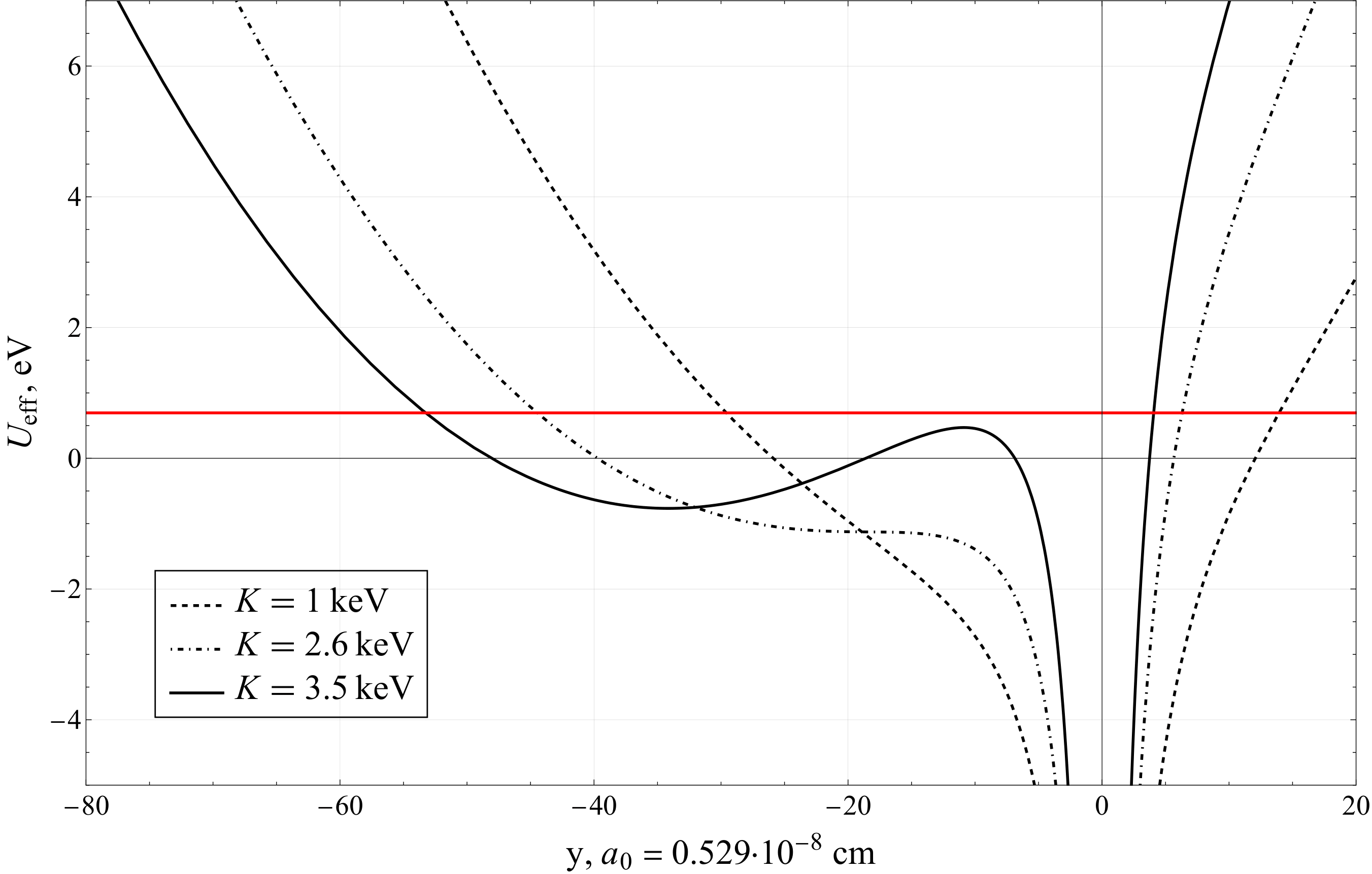
Figure 1: The effective potential (12) in eV as a function of y in $a_{0}=1/m_{e}e^{2}=0.529\cdot 10^{-8}$ cm for MF $\text{B}=6\cdot 10^{7}$ G, $\text{K}_{c}=2.61$ keV and three different values of K. The solid black horizontal line corresponds to $\text{E}=2m$, the red horizontal line to the ionization threshold $\text{I}=e\text{B}/m$.

IV The Energy Spectrum Equation

The spectral problem (II) for the Hamiltonian

$$\hat{\mathcal{H}}=\frac{\mathbf{K}^{2}}{4m}-\frac{1}{m}\Delta_{\bm{\eta}}-\frac{e}{2m}[\mathbf{K}\times\mathbf{B}]\cdot\bm{\eta}+\frac{e^{2}}{4m}[\mathbf{B}\times\bm{\eta}]^{2}-\frac{e^{2}}{|\bm{\eta}|}$$ (19)

does not admit an exact solution. For the exciton and the hydrogen atom moving in MF some analytical approximations has been developed [13, 16, 18, 19, 20]. Numerical calculations for Ps have been performed in [27, 28]. We wish to solve the problem relying on analytical methods as far as possible. Following [13, 20, 22] it is appropriate to use the «shifted» representation $\bm{\eta}^{\prime}=\bm{\eta}-\bm{\eta}_{c}$, where $\bm{\eta}_{c}$ is the difference between the coordinates of the gyro-motion guiding centers of $e^{+}$ and $e^{-}$

$$\bm{\eta}_{c} = \frac{\mathbf{K}_{1}\times\mathbf{B}}{e\text{B}^{2}}-\frac{\mathbf{K}_{2}\times\mathbf{B}}{-e\text{B}^{2}}=$$ (20)

$$=-\frac{[\mathbf{B}\times\mathbf{K}]}{e\text{B}^{2}}=-\frac{2m}{e\text{B}^{2}}[\mathbf{B}\times\mathbf{V}],$$

where $\mathbf{V}$ is given by (10). Note that with $\mathbf{B}$ directed along the $z$-axis $\eta_{cz}=0$. Henceforth we shall use the following notations: $\bm{\eta}^{\prime}=(\eta^{\prime}_{x},\eta^{\prime}_{y},z)\equiv(\bm{\rho}^{\prime},z)$, $\bm{\eta}_{c}=(\eta_{cx},\eta_{cy})\equiv\bm{\rho}_{0}$ and the coordinate $z$ is not affected by the shift. Inserting $\bm{\eta}^{\prime}=\bm{\eta}-\bm{\eta}_{c}$ into (19) one obtains the «shifted» Hamiltonian

$$\hat{\mathcal{H}}^{\prime} = \frac{\text{K}_{z}^{2}}{4m}-\frac{1}{m}\frac{\partial^{2}}{\partial z^{2}}-\frac{1}{m}\bigg{(}\frac{\partial^{2}}{\partial\eta_{x}^{\prime 2}}+\frac{\partial^{2}}{\partial\eta_{y}^{\prime 2}}\bigg{)}+$$ (21)

$$+\frac{e^{2}}{4m}\mathbf{B}^{2}\bm{\rho}^{\prime 2}-\frac{e^{2}}{\sqrt{(\bm{\rho}^{\prime}+\bm{\rho}_{0})^{2}+z^{2}}}.$$

The Stark term has been eliminated in this representation. The pseudomomentum $\mathbf{K}$ enters into (21) through $\bm{\rho}_{0}$ and only then via an explicit term $\text{K}^{2}_{z}/4m$. In strong MF when $\gamma=\text{B}/\text{B}_{a}\gg 1$, $a_{0}\gg\ell$ the Schrödinger equation with the Hamiltonian $\hat{\mathcal{H}}^{\prime}$ is best solved by the wave function expansion over the complete set of Landau orbitals [30] in the $\bm{\rho}^{\prime}$ plane. Retaining only lowest Landau level (LLL) we arrive at the adiabatic approximation [31, 32]

$$\varphi_{\mathbf{K}}(\bm{\rho}^{\prime},z)=R(\bm{\rho}^{\prime})f(z),$$ (22)

where $R(\bm{\rho}^{\prime})$ is the LLL wave function

$$R(\bm{\rho}^{\prime})=\frac{1}{\sqrt{2\pi}\ell}\exp\bigg{(}-\frac{\bm{\rho}^{\prime 2}}{4\ell^{2}}\bigg{)},$$ (23)

and $f(z)$ is a longitudinal part. Adiabatic approximation is increasingly accurate with $\gamma$ increasing. Substituting (22)–(23) into the Schrödinger equation $\hat{\mathcal{H}}^{\prime}\varphi_{\mathbf{K}}=\text{E}\varphi_{\mathbf{K}}$, acting by $\partial^{2}/\partial\bm{\rho}^{\prime 2}$ on $R(\bm{\rho}^{\prime})$, multiplying by $R(\bm{\rho}^{\prime})$ and integrating over $d\bm{\rho}^{\prime}$, we obtain

$$\frac{d^{2}f}{dz^{2}}+m\bigg{[}\text{E}-\frac{e\text{B}}{m}+\text{U}(z)\bigg{]}f(z)=0,$$ (24)

$$\text{U}(z)=\frac{e^{2}}{2\pi\ell^{2}}\iint\limits_{\mathbb{R}^{2}}d\bm{\rho}^{\prime}\frac{\exp(-\bm{\rho}^{\prime 2}/2\ell^{2})}{\sqrt{(\bm{\rho}^{\prime}+\bm{\rho}_{0})^{2}+z^{2}}}.$$ (25)

The term $\text{K}^{2}_{z}/4m$ in (21) does not influence the spectrum and is omitted.

Transition from the Schrödinger equation $\mathcal{H}^{\prime}\varphi_{\mathbf{K}}=\text{E}\varphi_{\mathbf{K}}$ with $\mathcal{H}^{\prime}$ given by (21) to (24) may be considered as averaging over the fast MF variables.

As already noted, $\text{I}=e\text{B}/m$ in (24) is zero-point energy of the LLL, or the ionization threshold. The energy E in (24) is given by

$$\text{E}=\text{I}+\text{E}_{\text{B}},$$ (26)

where $\text{E}_{\text{B}}$ is the binding energy. The sates with $(\text{E}-\text{I})<0$ are bound states corresponding to the closed channels. States with $(\text{E}-\text{I})>0$ lie above the ionization threshold and form a series of autoionizing resonances. With this definition (24) takes the form

$$\bigg{(}-\frac{1}{m}\frac{d^{2}}{dz^{2}}-\text{U}(z)\bigg{)}f(z)=\text{E}_{\text{B}}f(z).$$ (27)

V The Separated Potential Wells

According to (14) the outer potential well is formed when $\text{K}^{3}>\text{K}_{c}^{3}=(27/2)me^{3}\text{B}=(27/2)(1/a_{0}\ell^{2})$. Under this condition different configurations of the two potential wells and a barrier between them are possible. The shape of the resulting configuration dictates the most appropriate methods to solve eq.(24). The problem has three parameters with the dimension of length

$$a_{\text{B}}(\text{Ps})=2a_{0}=\frac{2}{me^{2}},\ell=\frac{1}{\sqrt{e\text{B}}},|\bm{\rho}_{0}|=|y_{0}|=\frac{\text{K}}{e\text{B}}.$$ (28)

Here $|y_{0}|$ is the absolute value of the projection of $\bm{\rho}_{0}=-[\mathbf{B}\times\mathbf{K}]/e\text{B}^{2}$ onto the $x=z=0$ plane and $\mathbf{K}=(\text{K},0,0)$ in this projection. Important to note that according to (18) $y_{0}=-\text{K}/e\text{B}$ coincides with the position of the MW minimum $y_{m}$ in the limit $\text{K}\gg\text{K}_{c}$. Therefore one can interpret $|y_{0}|$ as the distance from the bottom of the MW to the Coulomb center. The two wells, the Coulomb and the magnetic ones, are actually separated if $|y_{0}|\gg a_{\text{B}}(\text{Ps})$. The use of the adiabatic approximation (22) implies that $a_{\text{B}}(\text{Ps})\gg\ell$. We come to the conclusion that the conditions for the double-well regime in the adiabatic approximation are the following

$$\text{K}>\text{K}_{c},~{}~{}~{}~{}~{}|y_{0}|\gg a_{\text{B}}(\text{Ps})\gg\ell.$$ (29)

For the hydrogen atom the above situation was investigated in [18].

Next we return to eqs.(24)–(25). Inequalities (29) permit to take the square root out of the integral (25) at $\bm{\rho}=0$, i.e., at $y=0$ in the projection under consideration. Then (27) takes the form

$$\frac{d^{2}f}{dz^{2}}+m\bigg{(}\text{E}-\frac{e\text{B}}{m}+\frac{e^{2}}{\sqrt{y_{0}^{2}+z^{2}}}\bigg{)}f(z)=0.$$ (30)

The characteristic distance for the dynamics of $f(z)$ is $z\sim\ell$ while according to (29) $|y_{0}|\gg\ell$. Therefore the potential energy in (30) can be expanded in a series in powers of $z^{2}$. As a result (30) reduces to the linear oscillator equation, see Fig.2

$$\frac{d^{2}f}{dz^{2}}+m\bigg{(}\text{E}-\frac{e\text{B}}{m}+\frac{e^{2}}{|y_{0}|}-\frac{e^{2}}{|y_{0}|^{3}}\frac{z^{2}}{2}\bigg{)}f(z)=0.$$ (31)

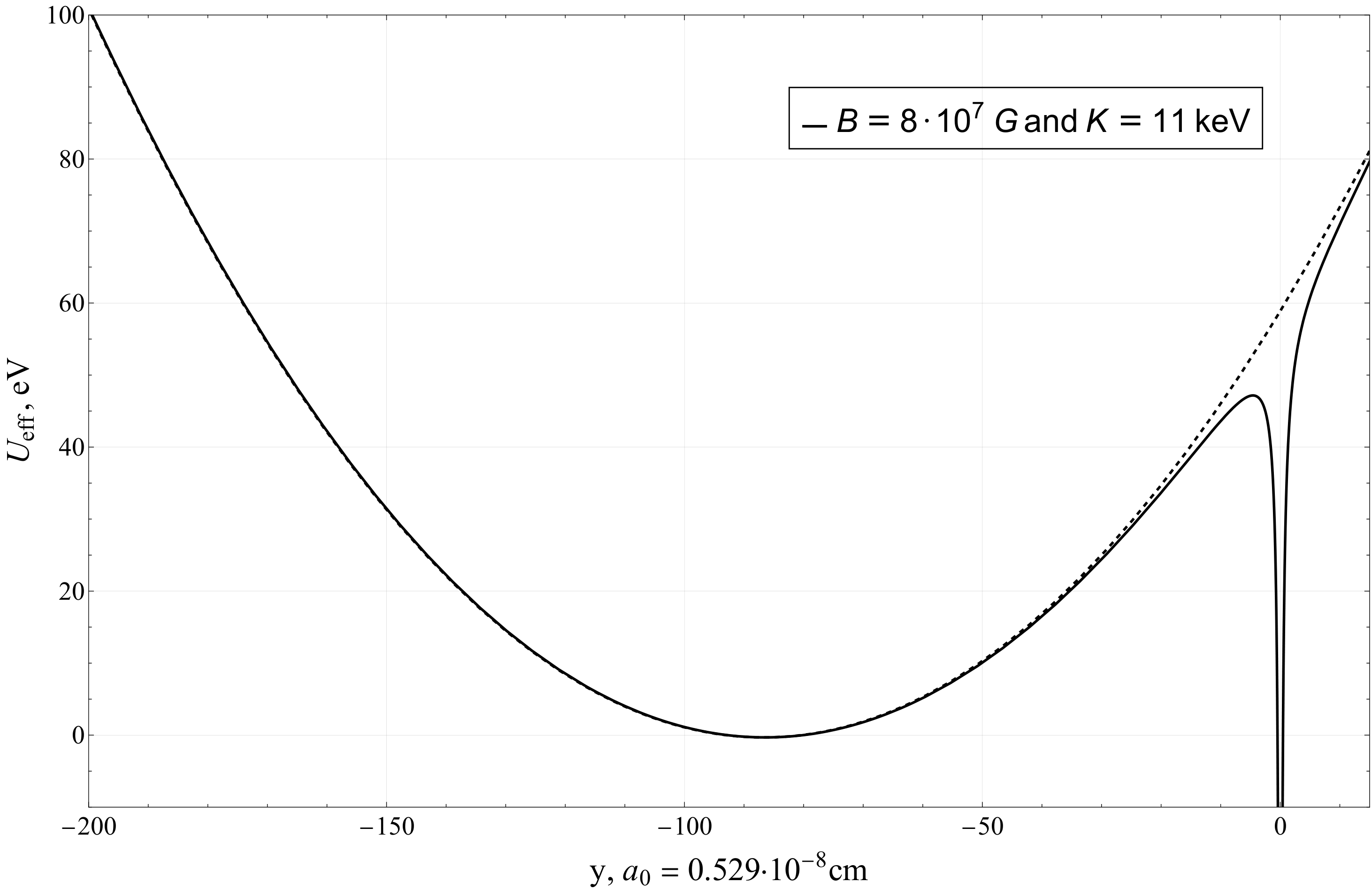
Figure 2: The illustrative plot of the oscillator approximation. The solid line is the projection of $\text{U}_{\text{eff}}$ on the $x=z=0$ plane. The dashed line is the parabolic approximation.

The energy levels are given by

$$\text{E}_{n}=\frac{e\text{B}}{m}-\frac{e^{2}}{|y_{0}|}+\bigg{(}n+\frac{1}{2}\bigg{)}\sqrt{\frac{2e^{2}}{m|y_{0}|^{3}}}.$$ (32)

It is instructive to express $\text{E}_{n}$ in atomic energy units $\text{a.u.}=2R_{\infty}=27.2\text{ eV}$. One has

$$\frac{\text{E}_{n}-e\text{B}/m}{\text{a.u.}} = -\frac{a_{\text{B}}(\text{Ps})}{2|y_{0}|}+$$ (33)

$$+\frac{1}{2}\bigg{(}\frac{a_{\text{B}}(\text{Ps})}{|y_{0}|}\bigg{)}^{3/2}\bigg{(}n+\frac{1}{2}\bigg{)}.$$

We remind that according to (29) $|y_{0}|\gg a_{\text{B}}(\text{Ps})$. Eq.(33) describes the spectrum in a wide, shallow parabolic potential. Imposing the condition $(\text{E}_{n}-e\text{B}/m)<0$ we conclude that (32)–(33) are valid up to

$$n\lesssim\sqrt{\frac{me^{2}\text{K}}{2(e\text{B})}}=\sqrt{\frac{|y_{0}|}{a_{\text{B}}(\text{Ps})}}.$$ (34)

Formally, beyond this restriction there is a condensation of infinite number of levels close to the ionization threshold. The transition from bound to autoionization states is far from being thoroughly studied [19, 33, 34].

The results of the ground states binding energies

$$\text{E}_{\text{B}}=\text{E}_{n=0}-\text{I}=-\frac{e^{2}}{|y_{0}|}\bigg{(}1-\frac{1}{2}\sqrt{\frac{a_{\text{B}}(\text{Ps})}{|y_{0}|}}\bigg{)}$$ (35)

are presented in Table 1. The characteristic bound states energies are of the order of a few eV.

Table 1: The energies of the lowest Landau states $\text{I}=e\text{B}/m$, $|y_{0}|=\text{K}/e\text{B}$ and the ground states binding energies $|\text{E}_{\text{B}}|$ for the MF in the range $(10^{10}-10^{14})$ G and $\text{K}>\text{K}_{c}$.

B, G	$10^{10}$	$10^{11}$	$10^{12}$	$10^{13}$	$10^{14}$
I, keV	0.12	1.16	11.6	115.8	1157.8
K, MeV	0.12	0.71	7.93	87.3	951.9
$|y_{0}|,a_{0}$	7.25	4.5	5.0	5.5	6.0
$|\text{E}_{\text{B}}|$, eV	2.77	4.03	3.72	3.45	3.22

VI The Overlapping Potential Wells

As already explained, the configuration of the potential depends upon the values of the four basic parameters: $\text{K},a_{\text{B}}(\text{Ps}),\ell,|\bm{\rho}_{0}|=|y_{0}|$ and on their dimensionless ratios. Under the condition (29) the outer well is formed, the adiabatic approximation is applicable and the two wells are isolated. Now we wish to consider the situation when the outer well is formed, the adiabatic approximation is valid but the two wells overlap. This corresponds to the following conditions

$$\text{K}>\text{K}_{c},~{}~{}~{}~{}~{}\ell\ll a_{\text{B}}(\text{Ps}),~{}~{}~{}~{}~{}|y_{0}|\ll a_{\text{B}}(\text{Ps}).$$ (36)

Note that we are not comparing $|y_{0}|$ and $\ell$ since their ratio depends on the value of K. In this section we partly rely on methods developed in [13, 35, 36, 37, 38, 39, 40].

Our task is to solve eq.(24) under the conditions (36). Firstly, we note that in the adiabatic approximation the size of Ps in the transverse plane is determined by the wave function (23) and is of the order of $\rho\sim\ell\ll a_{\text{B}}(\text{Ps})$. Therefore the density distribution of $|\varphi_{\mathbf{K}}(\bm{\rho},z)|^{2}$ takes the elongated shape in $z$-direction. This gives birth to the idea to replace the potential (25) by a MF independent one-dimensional potential. At $|z|\rightarrow\infty$ (25) has the following asymptotic form

$$\text{U}(z)\rightarrow\frac{e^{2}}{|z|}+\mathcal{O}\bigg{(}\frac{|y_{0}|^{2}}{|z|^{3}}\bigg{)}.$$ (37)

For (24) with the account of (26) this yields

$$\bigg{(}-\frac{1}{m}\frac{d^{2}}{dz^{2}}-\frac{e^{2}}{|z|}\bigg{)}f(z)=\text{E}_{\text{B}}f(z).$$ (38)

This is a one-dimensional Schrödinger equation with a Coulomb potential studied in [35, 36, 37, 38, 39, 40]. As a pure mathematical problem, eq. (38) does not have a complete set of solutions [38]. A way to overcome this problem is to remove the singularity at the origin by the use of a cut-off at $z=z_{0}$ [35, 36]. We follow an alternative approach of [37, 39]. Eq. (38) is solved inwards from $|z|=\infty$ and at $z=z_{0}$ the logarithmic derivative is matched with the same quantity of the approximate inner solution. This procedure lead to an equation for the energy spectrum.

It is convenient to change the variable $z$ to $\xi=2z/\nu a_{\text{B}}$ [35] with $\nu$ and $\xi$ being dimensionless. Whereupon (38) reduces to

$$\frac{d^{2}}{d\xi^{2}}f(\xi)+\bigg{[}\frac{1}{4}\bigg{(}m\nu^{2}a^{2}_{\text{B}}\bigg{)}\text{E}_{\text{B}}+\frac{\nu}{|\xi|}\bigg{]}f(\xi)=0,$$ (39)

or

$$\frac{d^{2}}{d\xi^{2}}f(\xi)+\bigg{(}-\frac{1}{4}+\frac{\nu}{|\xi|}\bigg{)}f(\xi)=0,$$ (40)

with $\nu$ related to the binding energy according to

$$\text{E}_{\text{B}}=-\frac{1}{ma_{\text{B}}^{2}\nu^{2}}.$$ (41)

Note that $\nu=1$ corresponds to $\text{E}_{\text{B}}=\text{E}_{0}\simeq-6.8$ eV the ground state energy of Ps. Eq. (40) is the Whittaker’s confluent hypergeometric equation [41]. The solution with positive $\nu$ that decreases exponentially at infinity is $f(\xi)=\text{const}\cdot W_{\nu,\nicefrac{{1}}{{2}}}(\xi)$. To match with the interior solution it suffices to keep the first order in $z$ terms. For $0<\nu\ll 1$ one can write [37]

$$W_{\nu,\nicefrac{{1}}{{2}}}\bigg{(}\frac{2z}{\nu a_{\text{B}}}\bigg{)}=-1+\frac{2z}{a_{\text{B}}}\bigg{(}\ln\frac{2z}{a_{\text{B}}}+\frac{1}{2\nu}+\mathcal{C}-1\bigg{)},$$ (42)

where $\mathcal{C}$ is the Euler constant ($\mathcal{C}=0.5772...$). The logarithmic derivative reads

$$\eta(\nu,z)_{\text{ext}} = \frac{\partial}{\partial z}\ln W_{\nu,\nicefrac{{1}}{{2}}}\bigg{(}\frac{2z}{\nu a_{\text{B}}}\bigg{)}=$$ (43)

$$=-\frac{1}{\nu a_{\text{B}}}-\frac{2}{a_{\text{B}}}\bigg{(}\ln\frac{2z}{\nu a_{\text{B}}}+\mathcal{C}\bigg{)}.$$

Next we consider the inner solution. The potential given by (25) is an even function of $z$ and hence the solutions may be either even or odd. We focus on even solutions leaving the odd ones for another publication. Following [37] we present the potential (25) in the following form

$$\text{U}(z)=\frac{e^{2}}{2\pi\ell^{2}}\iint d\bm{\rho}\frac{\exp(-\bm{\rho}^{2}/2\ell^{2})}{\sqrt{(\bm{\rho}+\bm{\rho}_{0})^{2}+z^{2}}}=$$

$$=\frac{e^{2}}{\ell}\vartheta\bigg{(}\frac{|z|}{\ell}\bigg{)},$$ (44)

where $\vartheta(\xi)$ is analytic for $|\xi|<\infty$. Introducing the variable $t=z/\ell$ we rewrite eq. (27) in the following form

$$\frac{d^{2}}{dt^{2}}f(t)+\bigg{(}\frac{2\ell}{a_{\text{B}}}\vartheta(t)-\frac{\ell^{2}}{a_{\text{B}}^{2}\nu^{2}}\bigg{)}f(t)=0,$$ (45)

where the expression (41) for $\text{E}_{\text{B}}$ has been used. Unlike the two and three dimensions for a one-dimensional Coulomb potential $\text{U}(|z|)=-e^{2}/|z|$ there is no continuity of the wave function and its derivative at $z=0$. Therefore in zero order we take $\ell=0$ (the infinite MF). In this case there are two solutions of (45)

$$f^{(0)}(t)=\text{const},~{}~{}~{}~{}~{}f^{(0)}(t)=\text{const}\cdot t.$$ (46)

The first one corresponds to even solution. To first order in $\ell$ we have the equation

$$\frac{d^{2}}{dt^{2}}f(t)+\frac{2\ell}{a_{\text{B}}}\vartheta(t)f^{(0)}(t)=0.$$ (47)

The solution reads

$$f(t)=\text{const}\bigg{(}1-\frac{2\ell}{a_{\text{B}}}\int\limits_{0}^{t}dt_{1}\int\limits_{0}^{t_{1}}dt_{2}\vartheta(t_{2})\bigg{)}.$$ (48)

For $f^{(0)}(t)=\text{const}$, i.e., for even states, the solution is finite and non-vanishing at $z=0$. Its logarithmic derivative is

$$\eta(z)_{\text{int}}=-\frac{2}{a_{\text{B}}}\int\limits_{0}^{z/\ell}\vartheta(t)dt,$$ (49)

where according to (44)

$$\vartheta(t)=\frac{1}{2\pi\ell}\iint d\bm{\rho}\frac{\exp(-\bm{\rho}^{2}/2\ell^{2})}{\sqrt{(\bm{\rho}+\bm{\rho}_{0})^{2}+z^{2}}}.$$ (50)

This is the point where the dependence on pseudomomentum K comes into play through $\bm{\rho}_{0}=-[\textbf{B}\times\textbf{K}]/e\text{B}^{2}$, or $y_{0}=-\text{K}/e\text{B}$, $\textbf{K}=(\text{K},0,0)$, see (28) above. Insertion of (50) into (49) yields

$$\eta(z)_{\text{int}}=-\frac{2}{a_{\text{B}}}\iint d\bm{\rho}\frac{\exp(-\bm{\rho}^{2}/2\ell^{2})}{2\pi\ell^{2}}\int\limits_{0}^{z/\ell}\frac{dt}{\sqrt{u^{2}+t^{2}}},$$ (51)

where $u^{2}=(\bm{\rho}+\bm{\rho}_{0})^{2}/\ell^{2}$. Integrating over $dt$ on obtains

$$\eta(z)_{\text{int}}=-\frac{2}{a_{\text{B}}}\iint d\bm{\rho}\frac{\exp(-\bm{\rho}^{2}/2\ell^{2})}{2\pi\ell^{2}}\bigg{[}\ln\bigg{(}1+$$

$$+\sqrt{1+\frac{(\bm{\rho}+\bm{\rho}_{0})^{2}}{z^{2}}}\bigg{)}+\ln\frac{z}{|\bm{\rho}+\bm{\rho}_{0}|}\bigg{]}=\mathcal{J}_{1}+\mathcal{J}_{2},$$ (52)

with $\mathcal{J}_{1}$ and $\mathcal{J}_{2}$ corresponding to the contribution of the first and second terms inside the square brackets. In the strong field limit $\ell\rightarrow 0$ and for $z/\ell\rightarrow\infty$ the integration of the first term is straightforward and gives $\mathcal{J}_{1}\simeq-(2/a_{\text{B}})\ln 2$. Evaluation of $\mathcal{J}_{2}$ is more complicated and is presented in the Appendix A. Summing the two contributions we obtain

$$\eta(z)_{\text{int}}=-\frac{2}{a_{\text{B}}}\bigg{(}\ln\frac{z}{\ell}+\frac{1}{2}\ln 2+\frac{1}{2}\ln\mathcal{C}+$$

$$+\frac{1}{2}\int\limits_{0}^{x}dt\exp(-t)\ln\frac{x}{t}\bigg{|}_{x=\frac{\ell^{2}\text{K}^{2}}{2}}\bigg{)}.$$ (53)

Equating the logarithmic derivatives (43) and (VI) we obtain the equation for $\nu$ of the Ps ground state

$$\frac{1}{\nu}+\ln\frac{1}{\nu^{2}} = \ln\frac{a_{\text{B}}^{2}}{2\ell^{2}}-\mathcal{C}-$$ (54)

$$-\int\limits_{0}^{x}dt\exp(-t)\ln\frac{x}{t}\bigg{|}_{x=\frac{\ell^{2}\text{K}^{2}}{2}}=$$

$$=\ln\gamma+\ln 2-\mathcal{C}-\Lambda\bigg{(}\frac{\ell^{2}\text{K}^{2}}{2}\bigg{)},$$

where $\gamma=\text{B}/\text{B}_{a}$, $\text{B}_{a}=m^{2}e^{3}=2.35\cdot 10^{9}\text{ G}$ is the atomic MF, $\Lambda(x)$ is the integral entering into (54). The derivation of (54) is based on the expansion (42) valid for $\nu\ll 1$ which corresponds to the ground state. The excited and odd states will be the subject of the forthcoming investigation. At $x\rightarrow 0$ the function $\Lambda(x)$ behaves as $\Lambda(x)\simeq x+\mathcal{O}(x^{2})$. For $\ell\text{K}\ll 1$ the term $\Lambda$ in (54) gives the following contribution to the ground state binding energy

$$\text{E}_{\text{B}}-\text{E}_{\text{B}0}=|\text{E}_{\text{B}0}|-|\text{E}_{\text{B}}|=\frac{1}{ma_{\text{B}}^{2}\nu_{0}}\bigg{(}\frac{\ell^{2}\text{K}^{2}}{2}\bigg{)},$$ (55)

where $\text{E}_{\text{B}0}$ and $\nu_{0}$ correspond to (54) with $\Lambda=0$. At $x\rightarrow\infty$ one has $\Lambda(x)\simeq\ln x+\mathcal{C}+\mathcal{O}(e^{-x})$. We remind that equation (54) for $\nu$ has been derived under the condition (36). Therefore the value of K can not be arbitrary large, namely $\text{K}\ell^{2}\ll a_{\text{B}}$, or $\text{K}\ll\gamma/a_{\text{B}}(\text{Ps}),\gamma=\text{B}/\text{B}_{a}$. For e.g. $\text{B}=10^{12}$ G the condition on K is $\text{K}\ll 3$ MeV.

For the neutral two-body system at rest in MF the eigenvalue equation (54) has been derived and treated by several authors most probably starting from [32]. In a refined form with a detailed discussion it was presented in [37] and later in [38]. The dependence on pseudomomentum in the form of the integral $\Lambda$ in (54) was given in [13] with a reference to [37]. It is interesting to see the relationship between (54) and the well-known result from Landau and Lifshitz [30] for the hydrogen ground state energy in MF. This estimate is logarithmically accurate and reads

$$\text{E}_{\text{B}}=-\frac{me^{4}}{2}\ln^{2}\frac{a_{\text{B}}^{2}(\text{H})}{\ell^{2}}.$$ (56)

To compare (56) with (54) we first recast (54) for the hydrogen. It amounts to the replacement of $a_{\text{B}}(\text{Ps})$ by $a_{\text{B}}(\text{H})$ and $m$ in (41) by $2m$ since the reduced mass of H is twice of Ps. Then we bring down (54) to the minimal form $1/\nu=\ln[a_{\text{B}}^{2}(\text{H})/2\ell^{2}]$ and obtain

$$\text{E}_{\text{B}}=-\frac{me^{4}}{2}\ln^{2}\frac{a_{\text{B}}^{2}(\text{H})}{2\ell^{2}},$$ (57)

which coincides with (56) with logarithmic accuracy. For Ps the same approximation yields for $\text{B}=10^{10}$ G

$$\text{E}_{\text{B}}=-\frac{me^{4}}{2}\ln^{2}\frac{a_{\text{B}}^{2}(\text{Ps})}{2\ell^{2}}\simeq-30\text{ eV}.$$ (58)

The numerical solution of (54) for this value of B and $\text{K}=0$ gives $\text{E}_{\text{B}}\simeq-9$ eV.

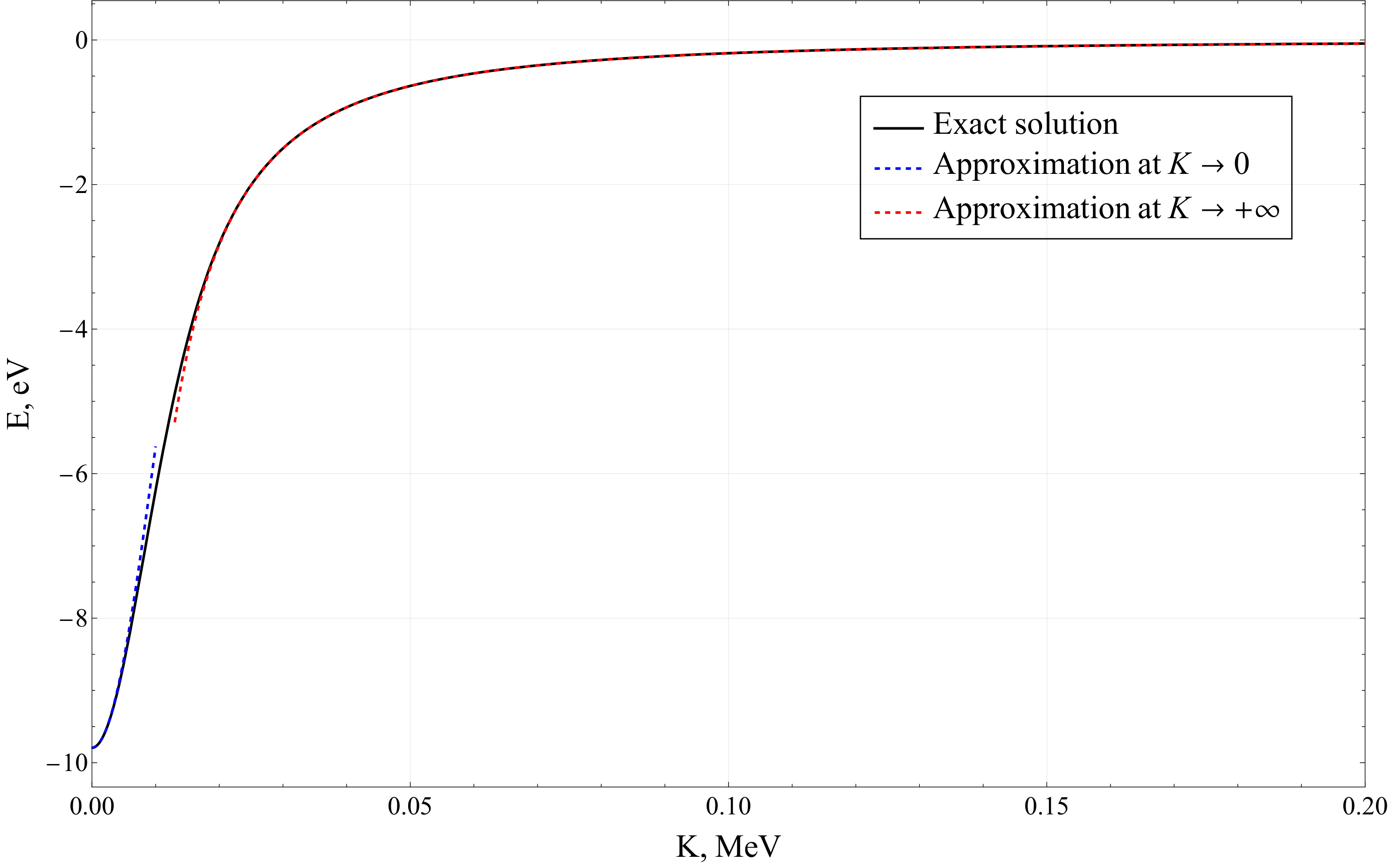
Figure 3: Dependence of the binding energy for the ground state (41) on the pseudo-momentum K. The blue dashed line corresponds to the limiting case of small K (75), the red line corresponds to the limiting case of large K (76). $\text{B}=10^{10}$ G.

The dependence of the Ps ground state binding energy on K is shown in Fig.3. The difference between the results of the Landau-type formula (58) and what gives the numerical solution of (54) is, as we see, considerable. The same is true for hydrogen where at $\text{B}=\text{B}_{\text{cr}}=m^{2}/e=4.414\cdot 10^{13}$ G (56) leads to $|\text{E}_{\text{B}0}|=1320$ eV while the exact calculation gives $|\text{E}_{\text{B}0}|=448$ eV [38].

As has been said in the Introduction, the main focus of our interest to the problem of Ps moving across a MF lies in the magnetospheres of NSs [8, 9, 10, 11]. Therefore it is necessary to present the result for the Ps moving in MF ground state energy obtained by solving the Bethe-Salpeter equation [10, 42]. Using the notation of the present work the result of [10, 42] reads

$$\text{E}_{\text{B}}=-\frac{me^{4}}{4}\ln^{2}\frac{a_{\text{B}}^{2}(\text{Ps})}{4\ell^{2}(1+\ell^{2}\text{P}_{x}^{2})}.$$ (59)

The gauge used by the authors is $A_{x}=-\text{B}y,A_{0}=A_{y}=A_{z}=0,\text{B}_{x}=\text{B}_{y}=0,\mathbf{B}=\mathbf{B}_{z}$. The gauge of the present work is $\mathbf{A}=1/2[\mathbf{B}\times\mathbf{r}]=1/2\cdot\text{B}(-y,x,0)$. The quantity $\text{P}_{x}$ is the transverse centre-of-mass momentum $\text{P}_{x}=p_{x}^{p}+p_{x}^{e}$ ($p_{x}^{p}$ refers to $e^{+}$ and $p_{x}^{e}$ to $e^{-}$) which is a constant of motion in the gauge of [10]. It is analogous to the pseudomomentum $\text{K}_{x}\equiv\text{K}$ of the present work through we are not immediately aware of the exact relation between the two. To find a bridge between (54) and (59) we take (54) in the following truncated form

$$\frac{1}{\nu}\simeq\ln\frac{a_{\text{B}}^{2}(\text{Ps})}{2\ell^{2}}-\Lambda\bigg{(}\frac{\ell^{2}\text{K}^{2}}{2}\bigg{)}.$$ (60)

At $\ell^{2}\text{K}^{2}/2\ll 1$ one has $\Lambda(x)\simeq x\simeq\ln(1+x)$ and (60) yields

$$\text{E}_{\text{B}}=-\frac{me^{4}}{4}\ln^{2}\frac{a_{\text{B}}^{2}(\text{Ps})}{2\ell^{2}(1+\ell^{2}\text{K}^{2}/2)},$$ (61)

which closely resembles (59). In the opposite limit of large $\ell^{2}\text{K}^{2}/2\gg 1$ one has $\Lambda(\ell^{2}\text{K}^{2}/2)\simeq\ln(\ell^{2}\text{K}^{2}/2)$. This leads to

$$\text{E}_{\text{B}}=-\frac{me^{4}}{4}\ln^{2}\frac{a_{\text{B}}^{2}(\text{Ps})}{\ell^{4}\text{K}^{2}}.$$ (62)

This corresponds to the limit $\ell^{2}\text{P}_{x}^{2}\gg 1$ in (59). We may draw a conclusion that our basic equation (54) and the result (59) from Bethe-Salpeter equation are neither identical nor contradictory to each other.

VII Implications

We have shown that the Ps wave function and the energy spectrum experience deep transformation as it moves through a MF. This carries far-reaching physical implications. Here we point out some new physical effects and postpone the detailed discussion for later. The first phenomenon to consider is the emergence of long-lived Ps [27, 28]. The Ps decay rate is proportional to the square of the wave function $|\psi(0)|^{2}$ evaluated at contact. For the MF strength $\text{B}\gg\Delta/4\mu_{0}=3.63$ T Ps has a maximum symmetry spin state with spin-down $e^{-}$ and spin-up $e^{+}$ [7, 30, 43, 44, 45]. Here $\Delta=8.4\cdot 10^{-4}$ eV is the hyperfine splitting, $\mu_{0}=5.79\cdot 10^{-5}\text{ eV}/\text{T}$ is the Bohr magneton. Therefore it is sufficient to consider only the coordinate part of the Ps wave function.

Accordingly to (22)–(23) the square of the Landau ground state wave function at $\bm{\eta}=\mathbf{r}_{1}-\mathbf{r}_{2}=0$, i.e., at $\bm{\rho}^{\prime}=-\bm{\rho}_{0},z=0$ reads

$$|\varphi_{\mathbf{K}}(0)|^{2} = \frac{1}{2\pi\ell^{2}}\exp\bigg{(}-\frac{\bm{\rho}_{0}^{2}}{2\ell^{2}}\bigg{)}f^{2}(0)=$$ (63)

$$=\frac{1}{2\pi\ell^{2}}\exp\bigg{(}-\frac{\text{K}^{2}\ell^{2}}{2}\bigg{)}f^{2}(0).$$

For the separated potential wells $f(z)$ satisfies the oscillator equation (31). The ground state solution is

$$f(z)=\bigg{(}\frac{m\omega}{\pi}\bigg{)}^{\nicefrac{{1}}{{4}}}\exp\bigg{(}-\frac{m\omega}{2}z\bigg{)},$$ (64)

where

$$\omega^{2}=\frac{2e^{2}}{m|y_{0}|^{3}}=\frac{2e^{2}}{m\text{K}^{3}\ell^{6}}.$$ (65)

Therefore

$$|\varphi_{\textbf{K}}(0)|^{2}=\frac{1}{2\pi\ell^{2}}\sqrt{\frac{m\omega}{\pi}}\exp\bigg{(}-\frac{\text{K}^{2}\ell^{2}}{2}\bigg{)}.$$ (66)

This has to be compared with $|\varphi(0)|^{2}=1/\pi a_{\text{B}}^{3}(\text{Ps})$ for Ps at rest without MF. From (66) it follows that the probability density at the origin exponentially drops for $\text{K}^{2}\ell^{2}/2\gg 1$. Recall that the outer potential well is formed when $\text{K}>\text{K}_{c}=(27/2a_{0}\ell^{2})^{\nicefrac{{1}}{{3}}}$. For $\text{B}=10^{12}$ G one has $\text{K}_{c}\simeq 70$ keV. When $\text{K}\gg\text{K}_{c}$ the square of the wave function at contact dramatically drops and Ps is actually stable against annihilation. As a side remark we mention that the parameter $\text{K}^{2}\ell^{2}/2$ in (66) enters also in the eigenvalue equation (54).

Another important property of the Ps decentered configuration is that it has a giant electric dipole moment [13, 27, 28, 42, 43]. From the physical considerations it is clear that the average distance between particles if given by the difference (20) between the coordinates of the gyro-motion guiding center of $e^{+}$ and $e^{-}$

$$\langle\bm{\eta}\rangle=\frac{\mathbf{K}_{1}\times\mathbf{B}}{e\mathbf{B}^{2}}-\frac{\mathbf{K}_{2}\times\mathbf{B}}{-e\mathbf{B}^{2}}=-\frac{\mathbf{B}\times\mathbf{K}}{e\mathbf{B}^{2}}.$$ (67)

Repeating the arguments that led to (12), consider the gauge $\text{K}_{y}=0,\mathbf{K}=(\text{K},0,0)$. Then $\langle\bm{\eta}\rangle_{y}=y_{0}=-\text{K}/e\text{B}$ and

$$d=ey_{0}=-\frac{\text{K}}{\text{B}}.$$ (68)

As noted before, and as it is clear from Fig.2, $y_{0}$ coincides with the position of the MW minimum at $\text{K}\gg\text{K}_{c}$. According to (29) in the configuration with the decentered MW $|y_{0}|\gg a_{\text{B}}(\text{Ps})$. It means that the dipole momentum can exceed by many orders of magnitude the value corresponding to the atomic unit of length. The Ps with a giant dipole moment plays an important role in the NS magnetosphere at the polar gap [42]. The electric field exerts a torque on the Ps dipole and causes it to rotate with angular velocity proportional to d. According to [42] this rotation prevents the increase of the distance between $e^{+}$ and $e^{-}$ and thereby prevents the ionization of Ps inside the polar gap.

Let us briefly touch upon a long standing contradictory problem of Ps one-photon annihilation in strong MF [44, 24, 25, 10, 45, 46]. The starting point of the discussion was Carr and Sutherland work [44]. The authors claimed that in MF the one-photon annihilation from the ground state of Ps is possible and calculated the corresponding rate. In [24] Wunner and Herold disputed this claim since in their view the state considered as a ground one in [44] was in fact an excited level. The analysis of [24] was based on the pseudomomentum formalism. The authors of [24] investigated the one-photon annihilation only from the $\mathbf{K}=0$ state. This state was self-evidently considered as a ground state of Ps. The conclusion of [24] was that one-photon annihilation from the Ps ground state is strictly forbidden.

We find it appropriate to shift the emphasis from the problem of one-photon annihilation from the $\mathbf{K}=0$ state to annihilation of Ps in the real physical conditions. We mean Ps moving across NS magnetosphere, or in AGN jets [43], or Ps in a strong laboratory MF. The relation between the centre-of-mass velocity $\mathbf{V}$, pseudomomentum $\mathbf{K}$, MF and the internal coordinate $\bm{\eta}$ is given by (10). This relation does not imply the physical reasons for the extra edge of the $\mathbf{K}=0$ state. As explained earlier, with the increase of K above the critical value, $\text{K}_{c}$ the Coulomb states are pushed above the ionization threshold and all of the bound states reside in the outer MW. The intersection of the photon dispersion line and the series of the Ps decentered states deserves a close attention.

VIII Summary and Future Prospects

We have investigated the transformation of the Ps wave function and energy spectrum taking place when Ps is moving through a MF. The main difference from the unmoving case is that the internal dynamics can not be separated from the centre-of-mass motion. The spectrum and the wave function parametrically depend on the generalized momentum operator $\mathbf{K}$ (4) also called pseudomomentum. When K exceeds the critical value (14) the outer «magnetic» potential well is formed in addition to the distorted Coulomb one. Two principal configurations are possible:

1. The separated Coulomb and outer potential wells with a potential barrier in between.

2. The overlapping wells with bilocalized wave function.

Both cases correspond to $\text{K}>\text{K}_{c}$ and to MF strong enough for adiabatic approximation to be legitimate

$$\gamma=\frac{\text{B}}{\text{B}_{a}}=\frac{\omega_{c}}{2R_{y}}\gg 1.$$ (69)

The first configuration corresponds to the relation (29) between the three main parameters $|y_{0}|$, $a_{\text{B}}(\text{Ps})$ and $\ell$. The second is realized under the condition (36). With K continuously increasing above $\text{K}_{c}$ the former Coulomb states are pushed above the ionization threshold and the spectrum resides in the decentered outer well. The character of this evolution depends on the value of MF. The states in the outer well have small annihilation rate and giant dipole moment.

Some interesting problems of Ps moving across MF remain for future studies. Among them is a bunch of questions relate to the possible transformation of photon into Ps in the pulsar magnetosphere [8, 9, 10, 11, 26, 43, 45]. As explained earlier it does not suffice to consider the one-photon annihilation from the $\mathbf{K}=0$ state. For this and for several other problems it is necessary to construct a kind of a wave packet made of different pseudomomentum values.

Another utmost interesting subject is magnetically stimulated Ps center-of-mass chaotic diffusion motion [47, 48, 49, 50]. Roughly speaking, the center-of-mass undergoes a transition from regular to Brownian motion if the internal motion changes from regular to chaotic. Worth mentioning that diffusion motion may be important for high precision experiments with antihydrogen atoms [49, 50].

IX Acknowledgments

The authors would like to thank M.A. Andreichikov for useful remarks and discussion.

Appendix A Calculation of the integral $\mathcal{J}_{2}$

Let’s transform the original expression for $\mathcal{J}_{2}$ to the following form

$$\mathcal{J}_{2} = \iint\limits_{\mathbb{R}^{2}}d^{2}\bm{\rho}\exp\bigg{(}-\frac{\bm{\rho}^{2}}{2\ell^{2}}\bigg{)}\ln\frac{z}{|\bm{\rho}+\bm{\rho}_{0}|}=$$ (70)

$$=2\pi\ell^{2}\ln\frac{z}{\ell}--\pi\ell^{2}\ln 2+\pi\ell^{2}C-$$

$$-\ell^{2}\int\limits_{0}^{\infty}\tau d\tau\exp(-\tau^{2})\mathcal{J}(\tau),$$

where $\mathcal{C}$ is Euler’s constant, numerically equal to $\mathcal{C}\simeq 0.57721$. By $\mathcal{J}(\tau)$ we mean the following integral

$$\mathcal{J}(\tau)=\int\limits_{0}^{2\pi}d\varphi\ln\bigg{(}1+\frac{2\rho_{0}}{\sqrt{2}\tau\ell}\cos\varphi+\frac{\rho_{0}^{2}}{2\tau^{2}\ell^{2}}\bigg{)},$$ (71)

which can be calculated by isolating the perfect square in the expression under the logarithm

$$\mathcal{J}(\tau) = \int\limits_{0}^{2\pi}d\varphi\ln\bigg{(}1+\frac{2\rho_{0}}{\sqrt{2}\tau\ell}\cos 2\varphi+\frac{\rho_{0}^{2}}{2\tau^{2}\ell^{2}}\bigg{)}=$$ (72)

$$=4\pi\ln\frac{|1-a|+1+a}{2}=$$

$$=\begin{cases}0,\text{ when }a<1\\ 4\pi\ln a,\text{ when }a\geq 1\end{cases},$$

where the notation $a=\rho_{0}/\sqrt{2}\tau\ell$ was introduced. Thus, integration over $\tau$ in $\mathcal{J}_{2}$ terminates at the value $\tau=\rho_{0}/\sqrt{2}\ell$, that is

$$\mathcal{J}_{2} = 2\pi\ell^{2}\ln\frac{z}{\ell}-\pi\ell^{2}\ln 2+\pi\ell^{2}\gamma-$$ (73)

$$-\ell^{2}\int\limits_{0}^{\rho_{0}^{2}/2\ell^{2}}dt\exp(-t)\ln\frac{\rho_{0}^{2}}{2t\ell^{2}}.$$

Appendix B Asymptotic behavior of function $\Lambda$

Function $\Lambda(x)$ has the form

$$\Lambda(x)=\int\limits_{0}^{x}dye^{-y}\ln\frac{x}{y}.$$ (74)

For small $x\rightarrow 0$ we have

$$\Lambda(x)=x+\mathcal{O}(x^{2}),~{}~{}~{}~{}~{}x\rightarrow 0,$$ (75)

where the fact was used that $df(x)/dx=(1/x)\int_{0}^{x}dye^{-y}\rightarrow 1$ for $x\rightarrow 0$. Taking the derivative in a similar way, in another limiting case $x\rightarrow+\infty$ we can obtain

$$\Lambda(x)=\ln x+\mathcal{C}+\mathcal{O}(e^{-x}),~{}~{}~{}~{}~{}x\rightarrow+\infty.$$ (76)

References

- Adkins et al. [2022] G. S. Adkins, D. B. Cassidy, and J. Perez-Rios, Phys. Rept. 975, 1 (2022).
- Karshenboim [2005] S. G. Karshenboim, Phys. Rept. 422, 1 (2005).
- Karshenboim [2004] S. G. Karshenboim, Int. J. Mod. Phys. A 19, 3979 (2004).
- Pokraka and Czarnecki [2017] A. Pokraka and A. Czarnecki, Phys. Rev. D 96, 9 (2017).
- Czarnecki [1999] A. Czarnecki, Acta Phys. Polon. B 30, 3837 (1999).
- Gninenko et al. [2006] S. N. Gninenko, N. V. Krasnikov, V. A. Matveev, and A. Rubbia, Phys. Part, Nucl 37, 321 (2006).
- Demidov et al. [2012] S. V. Demidov, D. S. Gorbunov, and A. A. Tokareva, Phys. Rev. D 85, 015022 (2012).
- Shabad and Usov [1982] A. E. Shabad and V. V. Usov, Nature 295, 215 (1982).
- Shabad and Usov [1985a] A. E. Shabad and V. V. Usov, JETP Letters 42, 19 (1985a).
- Shabad and Usov [1986] A. E. Shabad and V. V. Usov, Astrophys. Space Sci. 128, 377 (1986).
- Baring and Harding [2001] M. G. Baring and A. K. Harding, Ap. J. 547, 929 (2001).
- Lamb [Jr] W. E. Lamb(Jr), Phys. Rev. 85, 259 (1952).
- Gor’kov and Dzyaloshinskii [1968] L. P. Gor’kov and I. E. Dzyaloshinskii, Sov. Phys. JETP 26, 449 (1968).
- Grotch and Hegstrom [1971] H. Grotch and R. A. Hegstrom, Phys. Rev. A 4, 59 (1971).
- Avron et al. [1978] J. Avron, I. Herbst, and B. Simon, Annals of Physics 114, 431 (1978).
- Herold et al. [1981] H. Herold, H. Ruder, and G. Wunner, J.Phys. B: At. Mol. Phys. 14, 751 (1981).
- Andreichikov et al. [2019] M. A. Andreichikov, B. O. Kerbikov, and Y. A. Simonov, Physics-Uspekhi 62, 319 (2019).
- Burkova et al. [1976] L. A. Burkova, I. E. Dzyaloshinskii, G. E. Drukarev, and B. S. Monozon, Sov. Phys. JETP 44, 276 (1976).
- Dzyaloshinskii [1992] I. Dzyaloshinskii, Phys. Lett. A 165, 69 (1992).
- Baye et al. [1992] D. Baye, N. Clerbaux, and M. Vincke, Phys. Lett. A 166 (1992).
- Schmelcher and Cederbaum [1993] P. Schmelcher and L. S. Cederbaum, Chem. Phys. Lett. 208, 548 (1993).
- Potekhin [1998] A. Y. Potekhin, J. Phys. B: At. Mol. Opt. Phys. 31, 49 (1998).
- Lozovik and Volkov [2004] Y. E. Lozovik and S. Y. Volkov, Phys. Rev. A70 , 023410 (2004).
- Wunner and Herold [1979] G. Wunner and H. Herold, Astrophys. Space Sci. 63, 503 (1979).
- Wunner et al. [1981] G. Wunner, H. Ruder, and H. Herold, J. Phys. B: At. Mol. Phys. 14, 765 (1981).
- Herold et al. [1985] H. Herold, H. Ruder, and G. Wunner, Phys. Rev. Lett. 54, 1452 (1985).
- Ackermann et al. [1997] J. Ackermann, J. Shertzer, and P. Schmelcher, Phys. Rev. Lett. 78, 199 (1997).
- Shertzer et al. [1998] J. Shertzer, J. Ackermann, and P. Schmelcher, Phys. Rev. A58 , 1129 (1998).
- Alford and Strickland [2018] J. Alford and M. Strickland, Phys. Rev. D 88, 105017 (2018).
- Landau and Lifshitz [1978] L. D. Landau and E. M. Lifshitz, Quantum mechanics. Course of Theoretical Physics, vol. 3 (Pergamon Press, Oxford, 1978).
- Shiff and Snyder [1939] L. I. Shiff and H. Snyder, Phys. Rev. 55, 59 (1939).
- Elliot and Loudon [1960] R. J. Elliot and R. Loudon, J. Phys. Chem. Solids. 15, 196 (1960).
- Friedrich and Chu [1983] H. Friedrich and M. Chu, Phys. Rev. A 28, 1423 (1983).
- Friedrich and Wintgen [1989] H. Friedrich and D. Wintgen, Phys. Repf. 183, 37 (1989).
- Loudon [1959] R. Loudon, Amer. J. Phys. 27, 649 (1959).
- Loudon [2016] R. Loudon, Proc. R. Soc. A 472, 20150534 (2016).
- Hasegawa and Howard [1961] H. Hasegawa and R. E. Howard, J. Phys. Chem. Solids 21, 179 (1961).
- Popov and Karnakov [2014] V. S. Popov and B. M. Karnakov, Physics-Uspekhi 57, 257 (2014).
- Machet and Vysotsky [2011] B. Machet and M. I. Vysotsky, Phys. Rev. D 83, 025022 (2011).
- Godunov and Vysotsky [2013] S. I. Godunov and M. I. Vysotsky, Phys. Rev. D 87, 124035 (2013).
- Whittaker and Watson [1927] E. T. Whittaker and G. N. Watson, Modern Analysis. Cambridge, UK: Cambridge University Press (1927).
- Usov and Melrose [1996] V. V. Usov and D. B. Melrose, ApJ. 464, 306 (1996).
- Giblin and Shertzer [2012] J. T. Giblin and J. Shertzer, ISRN Astron. Astrophys. 2012 , 8484476 (2012).
- Carr and Sutherland [1978] S. Carr and P. Sutherland, Astrophys. Space Sci. 58, 83 (1978).
- Shabad and Usov [1985b] A. E. Shabad and V. V. Usov, Astrophys. Space Sci. 117, 309 (1985b).
- Leinson and Oraevskii [1985] L. B. Leinson and V. N. Oraevskii, SSor. J. Nucl. Phys. 42, 254 (1985).
- Schmelcher and Cederbaum [1992] P. Schmelcher and L. Cederbaum, Phys. Lett. A164, 305 (1992).
- Schmelcher [1992] P. Schmelcher, J. Phys. B: At Mol. Opt. Phys. 25, 2697 (1992).
- Dumin [2013] Y. V. Dumin, Phys. Rev. Lett. 110, 033004 (2013).
- Volponi [2023] M. Volponi, for AEgIS collaboration, Nuovo Cim. C46, 106 (2023).