Protecting Vehicle Location Privacy with Contextually-Driven Synthetic Location Generation
Abstract.
Geo-obfuscation is a Location Privacy Protection Mechanism used in location-based services that allows users to report obfuscated locations instead of exact ones. A formal privacy criterion, geo-indistinguishability (Geo-Ind), requires real locations to be hard to distinguish from nearby locations (by attackers) based on their obfuscated representations. However, Geo-Ind often fails to consider context, such as road networks and vehicle traffic conditions, making it less effective in protecting the location privacy of vehicles, of which the mobility are heavily influenced by these factors.
In this paper, we introduce VehiTrack, a new threat model to demonstrate the vulnerability of Geo-Ind in protecting vehicle location privacy from context-aware inference attacks. Our experiments demonstrate that VehiTrack can accurately determine exact vehicle locations from obfuscated data, reducing average inference errors by 61.20% with Laplacian noise and 47.35% with linear programming (LP) compared to traditional Bayesian attacks. By using contextual data like road networks and traffic flow, VehiTrack effectively eliminates a significant number of seemingly “impossible” locations during its search for the actual location of the vehicles. Based on these insights, we propose TransProtect, a new geo-obfuscation approach that limits obfuscation to realistic vehicle movement patterns, complicating attackers’ ability to differentiate obfuscated from actual locations. Our results show that TransProtect increases VehiTrack’s inference error by 57.75% with Laplacian noise and 27.21% with LP, significantly enhancing protection against these attacks.
1. Introduction
With the increasing availability of wireless connectivity and advances in positioning technologies, vehicles are heavily involved in various location-based services (LBS) such as navigation (Wang-WWW2017, ) and transportation systems (Qiu-TMC2020, ). These services often require vehicles to share their real-time locations with central servers, posing significant privacy risks, such as potential tracking and exposure of sensitive information like drivers’ home addresses (To-TMC2017, ). Consequently, ensuring the location privacy of vehicles in LBS applications is crucial.
The issue of location privacy in LBS has gained considerable attention over the past two decades. Many recent studies like (Yu-NDSS2017, ; Andres-CCS2013, ; Bordenabe-CCS2014, ) have focused on geo-obfuscation, a location privacy protection mechanism (LPPM) that allows users to report obfuscated locations instead of exact coordinates to servers. Notably, Andrés et al. (Andres-CCS2013, ) introduced a formal privacy criterion for geo-obfuscation, called geo-indistinguishability (Geo-Ind), which is extended from Differential Privacy (DP), requiring that nearby real locations remain indistinguishable based on their obfuscated representations.
Albeit effective in protecting sporadic location privacy, Geo-Ind is also known as a context-free privacy criterion (GAP2018, ), without considering the impact of contextual information on mobile users’ obfuscated locations. Such an assumption limits the applications of Geo-Ind in many practical scenarios, where mobile users’ mobility is highly impacted by the surrounding environments. Recent endeavors (LIAO2007311, ; Xu-WWW2017, ; Cao-ICDE2017, ; Emrich-ICDE2012, ; Li-Sigspatial2008, ; Arain-MTA2018, ; Cao-ICDE2019, ; Li-SigSpatial2017, ) have delved into exploring the vulnerabilities of Geo-Ind by taking into account the spatiotemporal correlation of users’ reported locations. As a countermeasure, some other data privacy works (Cao-ICDE2017, ; Cao-ICDE2019, ; Ghinita-Sigspatial2009, ; Xiao-SIGSAC2015, ) focus on devising new context-aware privacy criteria and solutions to protect users’ location data.
While elegant, those works mainly rely on explicit stochastic models such as Markov chains (Qiu-SIGSPATIAL2022, ), but they tend to overlook the implicit long-term correlation between locations that may be deeply embedded within the contextual data. In fact, the availability of vehicle traffic flow information is on the rise globally, especially within the urban and suburban contexts, sourced from road sensors and traffic cameras (Kashinath-IEEEAccess2021, ; Ide-TITS2017, ), mobile applications (Liu-JNCA2019, ), and official government or municipal websites (Qiu-SIGSPATIAL2022, ). This rich contextual data presents an opportunity for attackers to learn vehicles’ implicit mobility patterns over long-term periods. Leveraging this knowledge, attackers can potentially refine the accuracy of location inference attacks, even when the vehciles’ locations have been obfuscated.
Our Contributions. To fill the aforementioned research gap, in this paper, we aim to study new context-aware threat model to track vehicle locations and develop the countermeasure. Particularly, we focus on the scenario where the vehicle traffic flow information is available. By leveraging the recent fast advancement of deep neural networks, we aim to delve into the implicit relationships - both short-term and long-term - embedded in the vehicles’ location data using the traffic flow information, without depending on explicit stochastic models.
Contribution 1: New context-aware threat model “VehiTrack”
To demonstrate the vulnerability of Geo-Ind when protecting vehicles’ location privacy, we introduce a new threat model called VehiTrack. VehiTrack seeks to recover the actual locations of a vehicle from its obfuscated data during a journey. It operates in two phases: In Phase 1, VehiTrack applies Bayes’ formula, considering the vehicle’s mobility constraints over time on the road network, to estimate the real locations from obfuscated ones. In Phase 2, it uses Long Short-Term Memory (LSTM) neural networks, which are effective at recognizing both short-term and long-term correlation in sequence data, to refine these estimates using the vehicle traffic dataset. Our results show that VehiTrack significantly reduces the inference error by 61.51% and 48.15% compared to traditional Bayesian attacks when using Laplacian noise and linear programming (LP)-based geo-obfuscation methods, respectively.
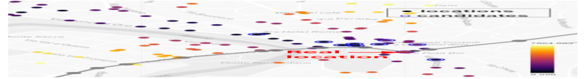
Our findings also reveal that the vulnerability of Geo-Ind to context-aware inference attacks largely stems from its failure to account for the constraints of road networks and traffic conditions on vehicle mobility. As depicted in Fig. 1(a), many locations within the obfuscation range, though compliant with Geo-Ind, are deemed “impossible” when contextual data is considered. This allows the VehiTrack model to significantly narrow its search for actual locations-on average, 81.69% of locations can be dismissed by incorporating road and traffic constraints. Motivated by this observation, we developed a new geo-obfuscation method called TransProtect. This approach ensures that the chosen obfuscated locations conform to realistic vehicle movement patterns, making it challenging for VehiTrack to effectively reduce the search range using contextual information.

Contribution 2: The countermeasure “TransProtect”
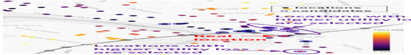
TransProtect is designed to create synthetic trajectories to closely emulate the vehicle’s actual mobility. As Fig. 1(b) shows, TransProtect can be integrated into the current geo-obfuscation framework to confine the obfuscation range to a set of locations within the generated synthetic trajectories, called “candidate locations”. Consequently, the obfuscated location chosen from candidate locations has to adhere to the realistic vehicles’ mobility patterns, which effectively prevents attackers from excluding any “impossible locations” using context-aware inference approaches like VehiTrack.
To create such synthetic trajectories, TransProtect leverages a transformer model, a deep neural network that learns context by handling long-range dependencies of the sequence data and has achieved great success in many artificial intelligence domains (lin2021survey, ; Chen-ICDE2023, ). To process the location sequence data of vehicles, we let TransProtect first conduct location embedding to map the node (location) set of the road network to a lower dimensional vector space, preserving spatial features of road network locations. To achieve this objective, TransProtect applies Node2Vec (grover2016node2vec, ) to maximize the log probability of observing a network neighborhood for each node conditioned on its feature representation. It also utilizes a Graph Convolutional Network (GCN) (kipf2017semisupervised, ) to integrate edge weights and neighborhood data into these embeddings.
TransProtect uses a Transformer encoder to evaluate each location’s likelihood of being the vehicle’s real position by capturing spatial patterns and adjusting scores based on data utility loss, then selects the top locations for obfuscation.
Contribution 3: Empirical validation based on real-world dataset
To evaluate the performance of both VehiTrack and
TransProtect, we conducted an extensive simulation using the Rome taxi trajectory datasets (roma-taxi-20140717, ), comparing both methods against state-of-the-art location inference and location privacy protection algorithms. The experimental results show that (1) When provided with vehicle locations obfuscated using Laplacian noise (Andres-CCS2013, ) and LP, VehiTrack demonstrates remarkable accuracy in tracking vehicle locations. On average, its expected inference error (EIE), which reflects the location privacy level, is 66.58% and 51.17% lower for Laplacian noise and LP (averaged on all epsilon values), respectively, compared to classic Bayesian inference attacks (Yu-NDSS2017, ). (2) Our proposed countermeasure, TransProtect, can effectively protect the location privacy of vehicles against VehiTrack. On average, the synthetic location set generated by TransProtect increases EIE by 40.26%
when using Laplacian noise and LP for obfuscation (Qiu-TMC2020, ; Shokri-CCS2012, ).
The rest of the paper is organized as follows: Section 2 gives the preliminaries of Geo-Ind. Section 3 introduces the new threat model VehiTrack and Section 4 describes the countermeasure TransProtect. Section 5 evaluates the performance of both VehiTrack and TransProtect. Section 6 presents the related work. Finally, Section 7 makes a conclusion.
2. Preliminary
In this Section, we introduce the preliminary knowledge of geo-obfuscation (Section 2.1), its privacy criterion Geo-Ind (Section 2.2), and the limitation of Geo-Ind (Section 2.3).
2.1. Geo-Obfuscation in LBS
To ensure the quality of LBS, the server needs to collect the participating vehicles’ location information in real-time. Like (Wang-WWW2017, ), we consider the scenario where the server is non-malicious but vulnerable to potential data breaches. In such scenarios, unauthorized parties might gain access to the reported vehicle locations stored on the server. Accordingly, the precise locations of the vehicles should be kept hidden from the server.
In geo-obfuscation (Andres-CCS2013, ; Bordenabe-CCS2014, ), privacy-conscious vehicles are allowed to use an obfuscation function to perturb their actual locations before reporting the locations to the server. The obfuscation function takes the vehicle’s precise location as the input and returns a probability distribution of the obfuscated location, based on which the vehicle can randomly select an obfuscated location to report. Beyond concealing the precise locations of vehicles, the obfuscated locations should be chosen in a manner that maintains the estimated travel cost to the destination reasonably close to the actual travel cost of the vehicle. Assessing the distortion of travel costs resulting from obfuscated locations requires access to global information about the target region, including its real-time vehicle traffic conditions and the distribution of spatial tasks. However, managing this data on an individual basis by vehicles poses significant challenges. As such, previous studies (Wang-WWW2017, ; Bordenabe-CCS2014, ; Qiu-TMC2020, ; Yu-NDSS2017, ) have mainly concentrated on the server-side computation of the obfuscation function.
For the sake of computational efficiency, many geo-obfuscation methods (Andres-CCS2013, ; Bordenabe-CCS2014, ) consider users’ mobility on a set of discrete locations. When considering vehicle LBS, the existing works (Qiu-TMC2020, ; Qiu-CIKM2020, ) discretize the road network into a set of road connections, denoted as . Those connections include road intersections, forks, junctions where roads intersect with others, and points where the road changes direction. All the other locations within the road network are approximated to their nearest connections in . By discretizing the location field into the finite location set , the obfuscation function can be described as an obfuscation matrix , where each denotes the probability of selecting as the obfuscated location given the actual location ().
2.2. Geo-Indistinguishability
Although the server takes charge of generating the obfuscation function, the vehicles’ exact locations are still hidden from the server since the obfuscated locations are selected in a probabilistic manner (Wang-WWW2017, ). Specifically, the obfuscation function is designed to satisfy Geo-Ind (Andres-CCS2013, ), which requires that even if an attacker has obtained a vehicle’s reported (obfuscated) location and the obfuscation function from the server, it is still hard for the attacker to distinguish the vehicle’s real location from any nearby location . Geo-Ind is formally defined in Definition 2.1:
Definition 2.0.
(Geo-Ind) An obfuscation matrix satisfies -Geo-Ind if, for each pair of neighboring locations with , the following constraints are satisfied
| (1) |
which means that the probability distributions of the obfuscated locations of and are sufficiently close. Here, denotes the Haversine distance (the angular distance on the surface of a sphere) between and , and is a predetermined distance threshold.
LP formulation. Many recent works (Wang-WWW2017, ; Qiu-TMC2020, ) address the quality issue caused by geo-obfuscation using linear programming (LP), of which the objective is to minimize the data quality loss while ensuring Geo-Ind is maintained. The LP is then formulated to optimize the values of , which comprises decision variables (entries). Besides satisfying Geo-Ind in Equ. (1), for each real location , the sum probability of the obfuscated locations should be 1 (probability unit measure), i.e.,
| (2) |
We let denote the utility loss caused by the obfuscation matrix , where is assumed to be a linear function of (Wang-WWW2017, ; Qiu-TMC2020, ). Finally, the LP is formulated to minimize while satisfying the constraints of the probability unit measure (Equ. (2)) and Geo-Ind (Equ. (1)):
| (3) |
2.3. Limitations of Geo-Ind
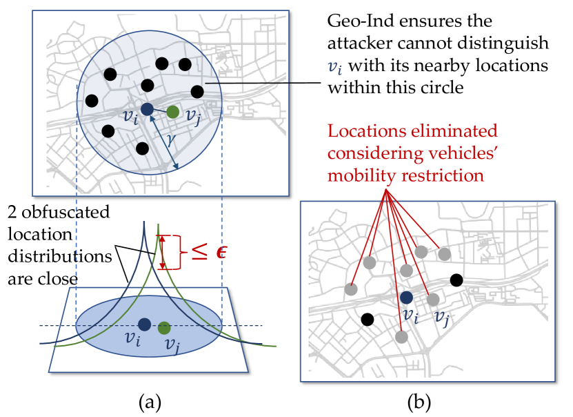
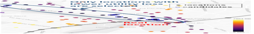
As Fig. LABEL:fig:GeoIndLimit(a) shows, Geo-Ind aims to guarantee that a vehicle’s location remains indistinguishable from any other location within the circle centered at with a radius of based on their obfuscated location distributions. However, Geo-Ind is a context-free privacy criterion without considering the context information that can be used in inference attacks. As Fig. LABEL:fig:GeoIndLimit(b) shows, an attacker can leverage context information, such as the vehicle’s historical locations, speed limits, and surrounding traffic conditions, to eliminate “impossible” locations of the vehicle within the circle. This, in turn, narrows down the search range for the vehicle’s actual location and increases the accuracy of its location tracking.
In the next section, we will introduce a new threat model to demonstrate the vulnerability of Geo-Ind when protecting vehicles’ location privacy.
3. VehiTrack: A Context-Aware Location Inference Algorithm
In this section, we introduce a new location inference algorithm, called VehiTrack, to accurately recover the real locations of a target vehicle from its obfuscated locations even though Geo-Ind has been satisfied.
We consider a scenario where a target vehicle reports its location multiple times at a sequence of time slots , where the actual locations and the obfuscated locations of the vehicle are denoted by and , respectively (, for each ). Given the observation of the vehicle’s obfuscated locations , VehiTrack aims to find the vehicle’s actual location sequence . To achieve this goal, VehiTrack consists of the following two main phases:
-
Ph1:
VehiTrack estimates the posterior of the vehicle’s location at each time slot , by considering the short-term correlation of the vehicle’s locations using a mobility
restriction-aware Bayesian inference model (Section 3.2). -
Ph2:
VehiTrack improves the accuracy of the posterior sequence , by considering the long-term correlation of the vehicle’s locations using Long Short-Term Memory (LSTM) neural networks (Section 3.1).
Before introducing the details of the above two phases, in Section 3.1, we first describe the mathematical models used in VehiTrack, including the main notations and assumptions.
3.1. Models
3.1.1. Threat model
To estimate the target vehicle’s true locations , we assume that the attacker has access to the following information at the time slots :
(1) the vehicle’s obfuscated locations ;
(2) the obfuscation matrices , where denotes the obfuscation matrix at time slot ;
(3) the background information including the vehicle’s mobility restrictions in the road networks (e.g., speed limits). We assume that the attacker has access to the public vehicle trajectory dataset (roma-taxi-20140717, ) to obtain historical traffic flow information.
For simplicity, we use to represent the prior probability that the vehicle is located at at time and use to represent the prior joint distribution of the vehicle being located at in the time slots .
3.1.2. Vehicle’s mobility model
We describe vehicles’ mobility in the road network as a directed graph , where and denote the node (location) set and the edge set, respectively. Each edge represents that is adjacent to in the road network, meaning that a vehicle can travel from to without visiting any other location in . Each edge is assigned a weight , representing vehicles’ minimum travel time through the edge . The shortest travel time from to (which are unnecessarily adjacent), denoted by , equals the length of the shortest path from to in . Here, the length of a path is defined as the sum weight of all the edges along the path.
Note that due to the change of traffic conditions (e.g., peak hours versus off-peak hours on weekdays), the edge weight can vary over time, rendering the mobility graph a time-varying graph. Given , we call a location is reachable by during a time interval if the shortest travel time from to during is no larger than , i.e., . We use to denote the set of locations reachable by (or called the reachable set of ) during .
3.2. Phase 1: Mobility Restriction-Aware Bayesian Inference
By leveraging the vehicles’ mobility restrictions and the obfuscation matrices, VehiTrack first estimates the posteriors of the target vehicle’s locations at the time slots via a Bayesian inference model. Note that deriving a posterior over the entire location set imposes a substantial computational burden. Indeed, due to the restrictions of the vehicle’s mobility and its limited obfuscation range, the possible true location of the vehicle can be confined to a smaller area. As a result, VehiTrack only needs to compute the posteriors of the locations within this reduced area and treat the posteriors of the locations outside this area as negligible.
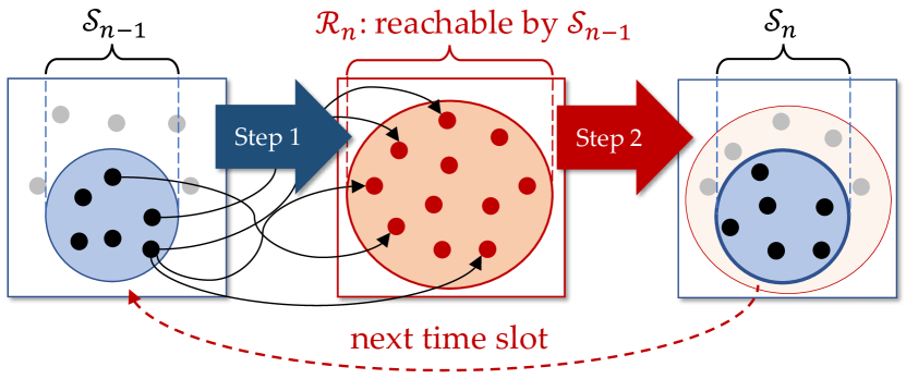
Step 1: Find the location set that are reachable by ;
Step 2: Derive the posterior of each location in and find the ones of which the posteriors are higher than the threshold .
We use to represent the set of the vehicle’s possible locations (identified by VehiTrack) at the time slot . Fig. LABEL:fig:BayesFramework shows the framework of how VehiTrack iteratively derives from , which is composed of the following two steps:
3.2.1. Step 1 - Identify the location set that is reachable by the locations in during the time interval
Here, is the union of the reachable sets of all the locations in , i.e., , i.e., each location in is reachable by at least one location in . To determine for each , VehiTrack builds a shortest path tree in the graph rooted at using the Dijkstra’s algorithm (Algorithm, ), of which the time complexity is . Here, represents the set of nodes included in the . For the sake of computation efficiency, VehiTrack limits to the location set of which the Haversine distance is no larger than , i.e., which are reachable by the vehicle with its maximum speed during without considering the mobility restriction imposed by the road network, i.e.,
| (4) |
VehiTrack first creates an induced subgraph of formed from the node set , where all of the edges (from ) connect pairs of vertices in . We then build on instead of the original graph .
Proposition 3.1.
is sufficient to identisfy .
Proof Sketch: We prove that for , if , then is included in , and also its distance to is equal to in . We prove it by contradiction, where the detailed proof can be found in Section A.1 in Appendix.
3.2.2. Step 2 - Determine the possible location set using the obfuscation matrices
Given the observed (obfuscated) location and the obfuscation matrix at each time slot , VehiTrack derives the posterior probabilities of all the locations using the Bayes’ formula:
| (5) |
Here, we consider as a “possible location” of the vehicle in only if its posterior value is higher than a pre-determined threshold . Therefore, is given by
| (6) |
3.3. Phase 2: Posterior Refinement using LSTM
Although VehiTrack considers the mobility restrictions of the target vehicle in adjacent time slots in Phase 1, it falls short of capturing the long-term correlation of the vehicle’s locations. In Phase 2, VehiTrack aims to further improve the accuracy of the posterior estimation by incorporating the LSTM networks, due to their strong capabilities of learning both short-term and long-term correlation in sequence data (Zhao-ITS2017, ). Specifically, VehiTrack takes the estimated posterior sequence obtained in Phase 1 as the inputs of the LSTM models and infers the real location sequence as the outputs. Achieving this goal entails training the LSTM model to establish the empirical relationship between the observed posteriors calculated by Phase 1 and the vehicle’s real locations.
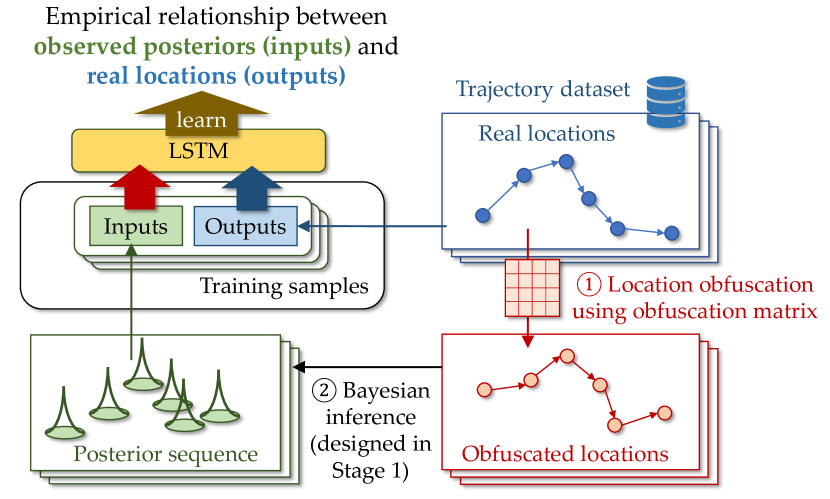
3.3.1. Training dataset generation
Following the threat model outlined in Section 1, we assume that the attacker has access to the historical vehicle mobility dataset in the region (Yan-Ubicomp2018, ). Moreover, we assume that the target vehicle follows similar mobility patterns with other vehicles in the dataset, despite potential individual variations. This allows VehiTrack to infer the target vehicle’s locations by LSTM trained by the historical vehicle mobility data.
VehiTrack generates training samples for an LSTM model by obfuscating real locations and using Bayesian inference to calculate location posteriors.
As Fig. LABEL:fig:Phase2trainingFramework shows, to obtain the training inputs (location posteriors), VehiTrack first obfuscates each real location in the trajectory using the obfuscation matrix (Step ①) and then derives the corresponding posteriors based on the obfuscated locations using the Bayesian inference model in Phase 1 (Step ②). The model is trained with one-hot encoded real locations as outputs, and multiple samples are created for each trajectory to reduce variance from the obfuscation process. To reduce the sample variance stemming from the stochastic obfuscated location selection process, we let VehiTrack generate multiple training samples (e.g., 20 samples in our experiments) for each trajectory.
3.3.2. LSTM network architecture
Fig. LABEL:fig:LSTMframework shows the framework of LSTM. The input posterior sequences undergo an initial processing step within the dimensionality management block. This block employs a padding method to enforce a standardized input format, specifically by aligning all trajectories with the longest one in the dataset. The padded posterior vectors are then passed to the neural network layer, a combination of 5 LSTM layers.
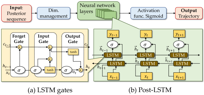
Fig. LABEL:fig:LSTMframework(a) and LABEL:fig:LSTMframework(b) illustrates our LSTM architecture, which, unlike conventional LSTM, processes entire posterior vectors instead of scalar values. This allows element-wise operations within the LSTM cells. We also use a BiLSTM model with two parallel layers (forward and backward) (huang2015bidirectional, ) to capture bidirectional patterns. The forget, input, and output gates dynamically manage the flow of information, deciding what to retain, add, or pass as the next hidden state.
To train Post-LSTM, we define the loss function as the cross entropy between predicted and actual vehicle location. The output of the neural network layer is directed to the sigmoid activation function block to constrain the output within the range . The result is then passed to the output block where an operation is performed upon the output to get the final estimation of the trajectory.
3.4. Performance of VehiTrack
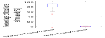
As demonstrated in our experiments detailed in Section 5.2, on average, using rome dataset (resp. using the San Francisco dataset), VehiTrack achieves a 65.54% and 45.93% (resp. 56.86% and 48.78%) reduction in inference errors corresponding to the Laplacian and Linear Programming methods respectively, compared to the classic Bayesian inference algorithm. Our findings also reveal that, by incorporating contextual information such as the road network and traffic flow, VehiTrack can eliminate a significant percentage of locations within the obfuscation range. For instance, in our experiment in Section 5, using rome dataset (resp. using the San Francisco dataset) on average, 81.99% (resp. 81.39) of locations within the obfuscation range are eliminated by considering vehicles’ mobility restrictions. This factor contributes significantly to the high inference accuracy performed by VehiTrack.
4. TransProtect: A Countermeasure of VehiTrack
As analyzed in Section 3, Geo-Ind proves susceptible to privacy breaches by VehiTrack when protecting the location privacy of vehicles. This vulnerability stems from the inclusion of “unrealistic” locations in its obfuscation range, which are prone to elimination by VehiTrack. Motivated by this insight, in this section, we introduce TransProtect, which aims to identify a set of “candidate obfuscated locations” that closely adhere to the realistic mobility patterns of vehicles, making them difficult for attackers to distinguish from actual locations.
4.1. The Framework of TransProtect
As illustrated by Fig. 6, TransProtect can be integrated into the current geo-obfuscation framework, such as LP-based geo-obfuscation (Qiu-TMC2020, ) or Laplacian noise (Andres-CCS2013, ). Using the context data including local historical traffic flow data and LBS target distributions, the server initially trains a “TransProtect” model (①). This model takes a vehicle’s trajectory as input and outputs a set of candidate obfuscated locations for the vehicle’s current location within the trajectory. Before reporting the location, each participating vehicle needs to download the trained “TransProtect” model to identify the candidate location set for obfuscation (②). Then, the vehicle can locally obfuscate its location within the candidate location set using Laplacian noise (③), which requires a low computational load that doesn’t necessitate global LBS service information. Alternatively, the vehicle can report the candidate location set, prompting the server to compute the obfuscation matrix using LP (②), which incurs a relatively higher computational load and relies on global target information. In both cases, The integration of TransProtect into the geo-obfuscation framework allows for the restriction of the obfuscation range to a specific set of locations, aligning with vehicles’ realistic mobility features while minimizing utility loss.
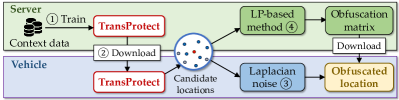
Fig. 7 shows the framework of TransProtect. TransProtect first takes the vehicle’s real location sequence (or the trajectory), , as the input. During each time slot , TransProtect assesses both the utility loss and the likelihood of each location being the actual location, based on the vehicle’s historical locations . After this assessment, TransProtect outputs a maximum of locations as the “candidate locations” for the obfuscated location, with representing the maximum allowable number of locations within the obfuscation range.
As shown by Fig. 7(a)(b)(c), TransProtect mainly comprises the following three components: (a) location embedding, (b) location assessment by transformer encoder, and (c) location ranking adjusted by utility loss. Next, we introduce the details of the three components in Section 4.2, Section 4.3, and Section 4.3, respectively.
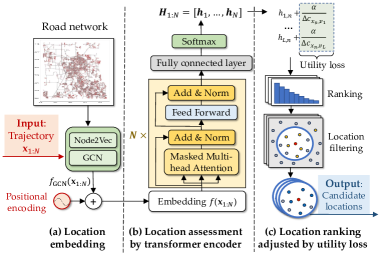
4.2. Location Embedding
The objective of location embedding is to map the nodes (locations) in the road network graph to a low dimensional feature space, where the neighborhood information of each node in can be well-preserved. Here, we let be the map from the locations to their feature representations, where denotes the dimension of the resulting embeddings.
Node2Vec. To achieve the above objective, as Fig. 7(a) shows, we first map locations to vectors using Node2Vec (grover2016node2vec, ), a semi-supervised algorithm designed for scalable feature learning in network structures. Node2Vec seeks to maximize the log-probability of observing a network neighborhood for each node conditioned on its feature representation , i.e.,
| (7) |
Directly minimizing the objective function in Equ. (7) results in significant computational overhead when the location set is large. Equ. (7) can be simplified to
| (8) |
by assuming the conditional independence of the likelihood of observing the neighbors in and the symmetry in feature space, where can be further approximated using negative sampling (NIPS2013_9aa42b31, ).
Graph Convolutional Network. Following the initial embedding of nodes via Node2Vec, we proceed to improve these embeddings using a Graph Convolutional Network (GCN) (kipf2017semisupervised, ). The primary goal of GCN is to incorporate both the edge weights and the neighborhood information into the node representations, thus achieving a more contextually comprehensive embedding.
Specifically, GCN processes the Node2Vec embeddings using a series of convolutional layers. Each layer in GCN updates the node embeddings by aggregating information from their respective neighborhoods, with an emphasis on the connectivity patterns as dictated by the graph structure. This process is formally expressed through the following convolution operation in each layer:
| (9) |
where denotes the symmetric normalized Laplacian matrix. Here, includes the addition of the identity matrix to incorporate self-connections , and is the diagonal node degree matrix of . The matrix represents the activations from the -th layer, is the layer’s trainable weight matrix, and is a non-linear activation function such as the sigmoid. The initial layer activations are set to the node embeddings .
By applying Node2Vec followed by GCN, we obtain the embedding of each trajectory , denoted as , which captures the spatial nuances of the trajectory within the embedding space.
Positional embedding. As Fig. 7(a) shows, after Node2Vec and GCN, each trajectory is initially transformed into a vector space representation . To incorporate the sequential order of the locations in the trajectory, positional encodings are added to the embedding vectors. These encodings provide a unique position signature that allows the model to consider the order of locations within each trajectory. The positional encodings are calculated as follows:
| (10) |
where and are the location’s position in the trajectory and the dimension index, respectively. These encodings are added to the embedding vectors to produce the final location embeddings .
4.3. Location Assessment by Transformer
As Fig. 7(b) shows, taking the location embeddings as the inputs, the transformer encoder in the second component outputs the score matrix , where each vector contains the predictive probability scores across all the locations in at each time slot . Here, is the number of locations in , and each probability score () reflects ’s likelihood of being the real location at given the observation of the vehicle’s historical locations .
Detailed steps of the Transformer encoder. As illustrated by Fig. 7(b), is first passed to a multi-head attention mechanism. In each attention head, the input sequence is linearly transformed into queries , keys , and values using respective weight matrices. The scaled dot-product attention for each head is computed as:
| (11) |
Each attention head processes the sequence independently using the following transformation:
| (12) |
The outputs from each head are then concatenated and linearly transformed to produce the final representation for each position in the sequence: .
Here, is the number of headers, and , , , and are the trainable parameters of the model. The dimensionality of each head’s output, , is set to to maintain a consistent dimensionality across different heads. After processing the sequence through the Transformer’s multi-head attention module, the derived representation is then delivered to a fully connected layer. This layer applies a learned linear transformation characterized by weight matrix and bias , producing a set of logits for each location in the sequence: , where represents the logits at time slot , and denotes the -th vector in the sequence after the attention mechanism. For each time step , the logits are then passed through a softmax function to yield a probability distribution over the set of all possible locations , i.e., . By stacking the vectors for all the time slots, we construct the probability score matrix . serves as the final output from the Transformer encoder, encapsulating the predictive distribution over the location set at each time step within the trajectory.
Loss and Training. During the training process, we aim to minimize the cross entropy loss between the predicted location probability distribution and the location ground truth (which is obtained from the real vehicle trajectory dataset (roma-taxi-20140717, )), i.e., .
Here, is a one-hot encoded matrix of the true locations with indicating the ground truth presence (or absence) of a location at time slot in the trajectory.
4.4. Location Ranking Adjusted by Utility Loss
As depicted in Fig. 7(c), after assessing the probability scores of the locations using the Transformer encoder, TransProtect adjusts the scores by the data utility associated with each location. Here, we use to denote the utility loss caused by the obfuscated location given the real location . Each location is assessed by the weighted sum of the probability score and the inverse of the utility loss: , where the weight is a predefined constant, reflecting the user’s emphasis on data utility during location obfuscation. TransProtect then ranks all the locations in based on their weighted scores and selects the top locations as the “candidate locations” for obfuscation.
Measurement of utility loss. The assessment of utility loss is contingent on the specific manner in which location data is used in downstream decision-making. As an example, in this paper, we consider the LBS applications where vehicles need to physically travel to designated locations to receive desired services such as navigation (To-TMC2017, ), or to fulfill tasks in spatial crowdsourcing (Qiu-TMC2020, ). In those applications, data utility loss can be quantified by the discrepancy between the estimated and actual travel costs to reach the designated locations. Note that our framework is also readily extended to other LBS applications with slight adjustments, provided that a clear relationship between data utility loss and obfuscated data can be established.
We let denote the prior probability that the target location is located at the location (). Given a real location , the utility loss caused by an obfuscated location is defined as the expected error of the traveling costs to the target location, calculated by
| (13) |
Location filtering. After calculating the weighted score of each location , TransProtect identifies the set of candidate locations using a min heap (Algorithm, ), mainly with the two features: (f1) the top element has the minimum score in the heap; (f2) the min heap has two types of operations: push to insert a new element, and pop to remove the top element from the heap. The min heap is initialized by empty. TransProtect then pushes each location in onto the heap. Once the heap reaches its capacity and determines whether to add a new location , TransProtect first checks whether the top location in the current heap has a higher score than . If NO, won’t be pushed onto the heap since it has a lower score than the locations in the current heap; If YES, the top location is popped off and is pushed onto the heap. Note that the popped location cannot have the highest score, since it has a lower score than the other locations in the current heap and the newly added location .
Time complexity. In min heap, both push and pop operations take time complexity and space complexity. Suppose that there are candidate locations to check by the transformer encoder. To find the locations with the highest scores, it takes up to push/pop operations, amounting to operations. As both and are not large in practice, e.g. they are set by up to 50 and 1739 respectively in our experiment (Section 5), such a computation load is acceptable to vehicle-equipped devices like smartphones.
5. Performance Evaluation
We carry out an extensive simulation to assess the performance of our location inference algorithm VehiTrack and our new LPPM TransProtect in Section 5.2 (Experiment I) and Section 5.3
(Experiment II), respectively, with the comparison of a list of state-of-the-art methods. In Section 5.1, we first introduce the settings of the experiment, including the real-world dataset used in the simulation, the benchmarks, and the performance metrics111The source code of both VehiTrack and TransProtect is available at: https://github.com/sourabhy1797/VehiTrack..
5.1. Experimental Settings
5.1.1. Vehicle location dataset
We adopt two vehicle trajectory datasets: (1) Rome taxicab dataset (roma-taxi-20140717, ), which includes 367,052 trajectories from approximately 320 taxis, covering 30+ days, and (2) San Francisco dataset (SanFranciscotaxi, ), including 34,564 trajectories from 536 taxis, covering 30 days. For both datasets, the road network information of the target region is extracted by OpenStreetMap (openstreetmap, ), which provides fine-grained location (node) and road (edge) information. To crop the road map data of Rome (resp. San Francisco), we compute the bounding area keeping a coordinate (latitude = 41.9028, longitude = 12.4964) (resp. (latitude = 37.7739, longitude = -122.4312)) as the center and computed all the nodes and edges within a 20-kilometer (resp. 10-kilometer) radius distance from the center.
5.1.2. TransProtect model training setting
The experiments are conducted on Ubuntu 22.04 with an NVIDIA GeForce 4090 GPU. We implement TransProtect using PyTorch 2.1 (PyTorch21, ). We set the embedding dimensionalities to 128 and batch size to 50. The initial learning rate is 0.001.
| Location privacy protection algorithms | ||||||||||||
| Location | Experiment I | Experiment II | ||||||||||
| inference | Laplace | Laplace+TransProtect | ||||||||||
| algorithms | Rome | San Francisco | Rome | San Francisco | ||||||||
| (km-1) | 5.0 | 7.5 | 10.0 | 5.0 | 7.5 | 10.0 | 5.0 | 7.5 | 10.0 | 5.0 | 7.5 | 10.0 |
| VehiTrack | 0.22 | 0.21 | 0.21 | 0.22 | 0.22 | 0.21 | 0.33(+53.4%) | 0.32(+49.2%) | 0.31(+46.6%) | 0.39(+74.5%) | 0.36(+64.22%) | 0.34(+58.6%) |
| VehiTrack-I | 0.63 | 0.62 | 0.62 | 0.31 | 0.31 | 0.30 | 0.66(+3.91%) | 0.65(+4.62%) | 0.65(+5.00%) | 0.53(+70.45%) | 0.53(+70.45%) | 0.52(+71.33%) |
| Bayes | 0.65 | 0.64 | 0.64 | 0.51 | 0.51 | 0.50 | 0.69(+5.80%) | 0.65(+1.92%) | 0.64(+0.49%) | 0.70(+36.79%) | 0.69(+35.54%) | 0.65(+29.42%) |
| HMM | 0.26 | 0.25 | 0.25 | 0.30 | 0.30 | 0.28 | 0.71(+175%) | 0.69(+179%) | 0.68(+176%) | 0.68(+124%) | 0.66(+121%) | 0.64(+130%) |
| Location privacy protection algorithms | ||||||||||||
| Location | Experiment I | Experiment II | ||||||||||
| inference | LP | LP+TransProtect | ||||||||||
| algorithms | Rome | San Francisco | Rome | San Francisco | ||||||||
| (km-1) | 5.0 | 7.5 | 10.0 | 5.0 | 7.5 | 10.0 | 5.0 | 7.5 | 10.0 | 5.0 | 7.5 | 10.0 |
| VehiTrack | 0.21 | 0.21 | 0.19 | 0.21 | 0.20 | 0.20 | 0.29(+34.9%) | 0.26(+24.9%) | 0.25(+32.7%) | 0.26(+22.43%) | 0.25(+23.73%) | 0.25(+24.58%) |
| VehiTrack-I | 0.30 | 0.26 | 0.25 | 0.32 | 0.31 | 0.32 | 0.39(+30.8%) | 0.35(+34.9%) | 0.33(+31.6%) | 0.44(+37.56%) | 0.42(+34.27%) | 0.40(+25.53%) |
| Bayes | 0.40 | 0.37 | 0.31 | 0.41 | 0.40 | 0.40 | 0.45(+14.2%) | 0.44(+19.5%) | 0.42(+32.7%) | 0.64(+53.96%) | 0.63(+54.70%) | 0.62(+56.64%) |
| HMM | 0.30 | 0.26 | 0.23 | 0.34 | 0.34 | 0.33 | 0.45(+50.3%) | 0.43(+65.6%) | 0.41(+78.1%) | 0.57(+67.51%) | 0.56(+64.26%) | 0.55(+66.01%) |
5.1.3. Benchmarks
In Experiment I, we test the performance of VehiTrack against the two conventional geo-obfuscation methods
(i) Planar Laplacian noise (labeled as “Laplace”) (Wang-WWW2017, ), which uses -Geo-Ind as the privacy criterion. Laplace assumes the obfuscation probabilities , where is the privacy budget, and is the maximum distance between any two locations in the target region.
(ii) LP-based geo-obfuscation (labeled as “LP”) (Qiu-TMC2020, ): LP (defined in Equ. (3)) aims to minimize the data utility loss of a single vehicle with the -GeoInd constraints being satisfied.
We compare the performance of VehiTrack with the following four classic location inference algorithms.
(i) Bayesian Inference attack (Yu-NDSS2017, ), labeled as “Bayes”: Given the vehicle’s obfuscated location, Bayes derives the posterior of the vehicle’s real location by the Bayes’ formula and estimates the vehicle’s real location as the location that maximizes the posterior.
(ii) Hidden Markov Model-based location inference (Qiu-SIGSPATIAL2022, ), labeled as “HMM”: HMM assumes the vehicle’s mobility follows a Markov process, of which the transition matrix can be learned explicitly using publicly accessible traffic flow data (Yan-IoTJ2022, ). In HMM, the vehicle’s real locations and obfuscated locations are considered hidden states and observable states, respectively. Under these assumptions, the vehicle’s real trajectory can be recovered from the obfuscated locations by the Viterbi algorithm (Viterbi-TIT1967, ).
(iii) VehiTrack in Phase 1, labeled as “VehiTrack-I”: To conduct an ablation study, we test VehiTrack-I, wherein the vehicles’ locations are inferred directly using the posterior sequence generated by Phase 1 of VehiTrack. A comparative analysis between VehiTrack and VehiTrack-I allows us to assess the extent of improvement attributed to the incorporation of LSTM in Phase 2.
In Experiment II, we integrate TransProtect into Laplace and LP, labeled as “Laplace+TransProtect” and “LP+TransProtect”, respectively. Specifically, we limit the obfuscation range of Laplace and LP to the candidate location set output by TransProtect. We test the four inference algorithms when vehicles’ locations are protected by “Laplace+TransProtect” and “LP+TransProtect”.
5.1.4. Metrics
In both Experiments I&II, we measure two metrics: (1) expected inference errors (EIE), which is defined as the expected error between the estimated locations (by attackers) and the vehicles’ actual locations, and (2) data utility loss, which is defined as the expected distortion of estimated traveling cost (in Equ. (13)).
5.2. Experiment I: Evaluation of VehiTrack
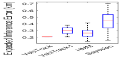
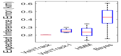
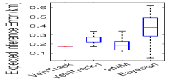
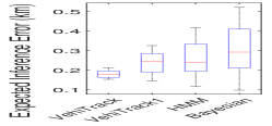
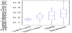
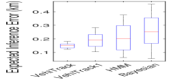
We randomly select 100 trajectories from the Rome and San Francisco Taxicab datasets to simulate the vehicles’ mobility. We use Laplace and LP to obfuscate all the locations within each trajectory, with locations recorded approximately every 20 seconds for both datasets. We then apply the four location inference algorithms, VehiTrack, VehiTrack-I, HMM, and Bayes to infer the vehicles’ real locations from the obfuscated locations, of which the expected inference errors are compared in “Experiment I” in Table 1 (Laplace) and Table 2 (LP). Based on the two tables, we have the following observations:
(1) Context-free location inference method Bayes has the highest inference error. On average, if we apply Laplacian noise as obfuscation methods, the inference error of Bayes is respectively 199.19%, 2.97%, and 156.33% (resp. 131.81%, 64.51%, and 70.00%) higher than that of VehiTrack, VehiTrack-I, and HMM using the Rome dataset (resp. using the San Francisco dataset). If we apply LP as obfuscation methods, the inference error of Bayes is 76.10%, 36.60%, and 36.65% (resp. 95.23%, 28.12%, and 36.66%) higher than that of VehiTrack, VehiTrack-I, and HMM using the Rome dataset (resp. using the San Francisco dataset). Unlike Bayes mainly focusing on single-location inference, the four context-aware inference methods achieve lower inference errors since they all account for the vehicles’ location correlation using either the road network mobility model (VehiTrack and VehiTrack-I) or Markov Model (HMM). In addition, Fig. 10 in Appendix shows that, on average, VehiTrack-I (and also VehiTrack) eliminates 81.69% (resp. 89.39%)of locations across 100 trajectories of Rome dataset (resp. San Francisco dataset) by considering vehicles’ mobility restrictions due to the road network. This substantial reduction aids attackers in narrowing down the search range for the vehicles’ actual locations.
(2) VehiTrack achieves an even lower expected inference error compared to the Markov-based method HMM. On average, using the Rome dataset (resp. the San Francisco dataset), the EIE of VehiTrack is 14.34% and 22.22% (resp. 26.66% and 38.23%) lower than that of HMM when Laplacian and LP are applied, respectively. HMM has higher inference error because assuming Markov property in HMM can only capture the correlation of vehicles’ locations in adjacent time slots (short-term), while LSTM in Phase 2 of VehiTrack can additionally capture the long-term correlations of vehicles’ locations, further improving the VehiTrack’s inference accuracy.
(3) VehiTrack outperforms VehiTrack-I in terms of inference accuracy (Ablation study). By comparing VehiTrack and VehiTrack-I, we find that LSTM in Phase 2 further reduces the average inference error by 65.58% and 24.12% for the Rome dataset and by 29.03% and 34.37% for the San Francisco dataset, considering both obfuscation methods (Laplacian noise and LP). Like HMM, VehiTrack-I achieves higher inference error, since it only captures short-term correlations within the location sequence by considering vehicles’ mobility restrictions due to the road network conditions, but without considering long-term correlation between locations.
To demonstrate that VehiTrack can better capture the long-term correlation of vehicles’ locations compared to the benchmarks, among the 100 trajectories, we pick up trajectories that have more than 40 locations. In Fig. 10(a)(b)(c) and Fig. 10(a)(b)(c) in Appendix, we exclusively evaluate the inference errors of the four algorithms for these selected “long” trajectories. The depicted results in the figure highlight that the accuracy advantage of VehiTrack is even more significant compared to the findings in Table 1 and Table 2, e.g., using the Rome dataset (resp. San Francisco dataset), VehiTrack’s inference error is 51.36%, 33.33%, and 48.56% (resp. 41.93%, 25%, and 29.16%) lower than that of Bayes, VehiTrack-I, and HMM, respectively (consider that for all the 100 trajectories of rome dataset, VehiTrack’s inference error is 49.77%, 41.41%, and 41.52% lower than that of Bayes, VehiTrack-I, and HMM, respectively).
| Location privacy protection algorithms | ||||||||
| Exp. I | Exp. II | |||||||
| (km-1) | Laplace | LP | Lap.+TransP. | LP+TransP. | ||||
| RM | SF | RM | SF | RM | SF | RM | SF | |
| 5.0 | 0.24 | 0.29 | 0.53 | 0.50 | 0.25 | 0.31 | 0.58 | 0.43 |
| 7.5 | 0.24 | 0.28 | 0.47 | 0.43 | 0.25 | 0.30 | 0.49 | 0.42 |
| 10.0 | 0.24 | 0.28 | 0.29 | 0.40 | 0.24 | 0.30 | 0.38 | 0.40 |
(4) As increases, the inference errors of all four inference algorithms increase. This is attributed to higher values of allowing for smaller deviations from obfuscated locations to actual locations. Consequently, this leads to a reduction in overall inference errors and also a lesser loss of data utility due to Laplacian noise and Linear Programming, as demonstrated in Table 3.
5.3. Experiment II: Evaluation of TransProtect
We apply TransProtect to refine the location set of geo-obfuscation and then assess the inference error of the four location inference algorithms, of which the results are shown in “Experiment II” in Table 1 (Laplace) and Table 2 (LP). By comparing the experimental results in Experiments I and II, we can check how much privacy improvement is contributed by TransProtect. In the tables, the subscript (+a%) means the inference error is increased by after integrating TransProtect. We have the following observations:
(1) Integrating TransProtect in Laplace and LP increases the expected inference error of the context-aware inference algorithms. On average, employing TransProtect increases the inference error of VehiTrack, VehiTrack-I, and HMM by 40.28%, 18.39%, and 119.41% (resp. 65.77%, 70.74%, and 125%) using Rome dataset (resp. San Francisco dataset). This is because the obfuscation range is restricted to the candidate locations (determined by TransProtect) that are difficult to distinguish from real locations using context-aware inference models. Particularly, Fig. 10(a)(b) in Appendix shows that with TransProtect integrated, on average using Rome dataset (resp. San Francisco), only 1.45% (resp. 1.59%) locations are eliminated in the obfuscation range by VehiTrack-I when vehicles’ mobility restrictions are considered, making it difficult for attackers to narrow down the search range for the target locations.
(2) The integration of TransProtect maintains the utility loss at an acceptable level. This is attributed to TransProtect’s inclination to choose locations with lower data utility loss, considering road network conditions. In contrast, the original obfuscation methods (i.e. Laplacian and LP) don’t consider measuring data utility loss in the road network when selecting obfuscated locations. Consequently, TransProtect allows the selection of locations further away from the real location, with the data utility loss guaranteed at an acceptable level (as shown in Table 3, i.e., on average, using Rome dataset (resp. San Francisco dataset), TransProtect increases the data utility loss by 1.04, 1.02, 1.30 times (resp. all 1.07) when 5.0km-1, 7.5km-1, and 10.0km-1.
6. Related Works
Geo-Ind. The discussion of location privacy criteria dates back nearly two decades to when Gruteser and Grunwald (Gruteser-MobiSys2003, ) introduced location -anonymity, based on Sweeney’s -anonymity (Sweeney2002, ). Recently, Andr’es et al. (Andres-CCS2013, ) extended Differential Privacy (DP) to ”Geo-Ind” for location privacy protection, spurring the development of new geo-obfuscation methods (Shokri-CCS2012, ; Andres-CCS2013, ; Wang-WWW2017, ; Yu-NDSS2017, ). For instance, Andr’es et al. (Andres-CCS2013, ) developed a geo-obfuscation method adding noise from a polar Laplacian distribution to actual locations to achieve Geo-Ind. Considering the diverse sensitivity of data utility loss to obfuscation in LBS, other works discretize the location domain and optimize the obfuscation distribution using LP (Bordenabe-CCS2014, ; Wang-WWW2017, ; Qiu-TMC2020, ; Qiu-CIKM2020, ; Qiu-ICDCS2019, ).
Context-aware threat models. Although effective in protecting sporadic locations, geo-obfuscation based on Geo-Ind is still vulnerable to context-aware inference attacks. Recent efforts have focused on attacking Geo-Ind using the spatiotemporal correlation of users’ reported locations, either from a single user over time (e.g., trajectory) (LIAO2007311, ; Xu-WWW2017, ; Cao-ICDE2017, ; Emrich-ICDE2012, ; Li-Sigspatial2008, ; Arain-MTA2018, ) or from multiple users (Cao-ICDE2019, ; Li-SigSpatial2017, ). Some works assume users’ mobility follows a Markov process (LIAO2007311, ; Emrich-ICDE2012, ), where current locations depend on previous ones, e.g., our prior work (Qiu-SIGSPATIAL2022, ) tracks vehicles’ locations using an HMM, where we learn the transition matrix of the Markov chain via publicly accessible traffic flow data.
Context-aware LPPM. Another approach to context-aware location privacy focuses on new privacy criteria and solutions to protect users’ location data (Cao-ICDE2017, ; Cao-ICDE2019, ; Ghinita-Sigspatial2009, ; Xiao-SIGSAC2015, ). For instance, assuming attackers use Markov models for users’ mobility, Cao et al. (Cao-ICDE2017, ) defined a criterion to quantify privacy levels of existing methods. Cao et al. (Cao-ICDE2019, ) extended DP to new criteria for spatiotemporal event privacy and created a framework to calculate privacy loss in location protection mechanisms. Considering temporal correlations, Xiao et al. (Xiao-SIGSAC2015, ) introduced -location set-based DP and a planar isotropic mechanism for geo-obfuscation. In (Qiu-SIGSPATIAL2022, ), we proposed generating synthetic trajectories using Markov chain, making it harder for attackers to distinguish real from obfuscated locations using traffic flow information. While elegant, context-aware threat models and LPPMs primarily rely on explicit stochastic models like Markov chains, overlooking long-term correlations between locations hidden in context data. In contrast, VehiTrack and TransProtect use DNNs to uncover implicit relationships in sequence data, outperforming existing methods in location inference and privacy protection.
Synthetic data-based privacy protection. It is worth mentioning that several recent works have used synthetic data to protect users’ privacy, especially in high-dimensional, sparse datasets prone to breaches (arnold2021really, ; choi2018generating, ; Drechsler-JASA2010, ; opendatainstitute, ; UKGovernment, ; xu2019modeling, ; Yale2019PrivacyPS, ). These studies focus on anonymization, preserving the statistical properties of original data while hiding users’ identities (choi2018generating, ) to protect personally identifiable information. In contrast, TransProtect uses synthetic data to increase indistinguishable pairs in the protected dataset, leading to different research challenges due to the divergent goals.
7. Discussions and Conclusions
In this work, we studied the context-aware location privacy protection for vehicles in LBS. We introduced a new threat model VehiTrack to show the vulnerability of Geo-Ind. As a countermeasure, we then developed TransProtect to create candidate locations for obfuscation that are hard to distinguish from real locations (by VehiTrack). The simulation results have demonstrated the vulnerability of Geo-Ind to VehiTrack and the effectiveness of TransProtect in protecting vehicles’ location privacy against VehiTrack.
We envision new promising research directions to explore further. In addition to LSTM, transformer models provide an alternative method for VehiTrack to track the locations of vehicles. Transformer has demonstrated its strong capability not only in synthetic data generation but also in a variety of inference models (CHITTYVENKATA2023102990, ). However, incorporating Transformer into VehiTrack introduces some additional challenges to address. First, we will study how to use Multimodal Transformers (xu2023multimodal, ) instead of Vanilla transformers, considering the different modalities in VehiTrack’s input (location posterior sequence) and output (location sequences). Before directing location posteriors into the Transformer model, we will apply approximation or discretization techniques to map posterior sequences to lower dimensional feature space considering their high dimensions.
8. Acknowledgements
The research was partially sponsored by the Army Research Laboratory and was accomplished under Cooperative Agreement Number W911NF-23-2-0014. The views and conclusions contained in this document are those of the authors and should not be interpreted as representing the official policies, either expressed or implied, of the Army Research Laboratory or the U.S. Government. The U.S. Government is authorized to reproduce and distribute reprints for Government purposes, not withstanding any copyright notation herein. This research was partially supported by U.S. NSF grants CNS-2136948 and CNS-2313866.
References
- [1] L. Wang, D. Yang, X. Han, T. Wang, D. Zhang, and X. Ma. Location privacy-preserving task allocation for mobile crowdsensing with differential geo-obfuscation. In Proc. of ACM WWW, pages 627–636, 2017.
- [2] C. Qiu, A. C. Squicciarini, C. Pang, N. Wang, and B. Wu. Location privacy protection in vehicle-based spatial crowdsourcing via geo-indistinguishability. IEEE Transactions on Mobile Computing, pages 1–1, 2020.
- [3] H. To, G. Ghinita, L. Fan, and C. Shahabi. Differentially private location protection for worker datasets in spatial crowdsourcing. IEEE Transactions on Mobile Computing, pages 934–949, 2017.
- [4] L. Yu, L. Liu, and C. Pu. Dynamic differential location privacy with personalized error bounds. In Proc. of IEEE NDSS, 2017.
- [5] M. E. Andrés, N. E. Bordenabe, K. Chatzikokolakis, and C. Palamidessi. Geo-indistinguishability: Differential privacy for location-based systems. In Proc. of ACM CCS, pages 901–914, 2013.
- [6] N. E. Bordenabe, K. Chatzikokolakis, and C. Palamidessi. Optimal geo-indistinguishable mechanisms for location privacy. In Proc. of ACM CCS, pages 251–262, 2014.
- [7] Chong Huang, Peter Kairouz, Xiao Chen, Lalitha Sankar, and Ram Rajagopal. Generative adversarial privacy, 2018.
- [8] L. Liao, D. J. Patterson, D. Fox, and H. Kautz. Learning and inferring transportation routines. Artificial Intelligence, 171(5):311 – 331, 2007.
- [9] F. Xu, Z. Tu, Y. Li, P. Zhang, X. Fu, and D. Jin. Trajectory recovery from ash: User privacy is not preserved in aggregated mobility data. In Proc. of ACM WWW, page 1241–1250, 2017.
- [10] Yang Cao, Masatoshi Yoshikawa, Yonghui Xiao, and Li Xiong. Quantifying differential privacy under temporal correlations. In Proc. of 2017 IEEE 33rd International Conference on Data Engineering (ICDE), pages 821–832, 2017.
- [11] T. Emrich, H. Kriegel, N. Mamoulis, M. Renz, and A. Zufle. Querying uncertain spatio-temporal data. In Proc. of IEEE ICDE, pages 354–365, 2012.
- [12] Q. Li, Y. Zheng, X. Xie, Y. Chen, W. Liu, and W. Ma. Mining user similarity based on location history. In Proc. of SIGSPATIAL, 2008.
- [13] Qasim Ali Arain, Imran Memon, Zhongliang Deng, Muhammad Hammad Memon, Farman Ali Mangi, and Asma Zubedi. Location monitoring approach: Multiple mix-zones with location privacy protection based on traffic flow over road networks. Multimedia Tools Appl., 77(5):5563–5607, mar 2018.
- [14] Y. Cao, Y. Xiao, L. Xiong, and L. Bai. Priste: From location privacy to spatiotemporal event privacy. In Proc. of IEEE ICDE, pages 1606–1609, 2019.
- [15] W. Li, H. Chen, W. Ku, and X. Qin. Scalable spatiotemporal crowdsourcing for smart cities based on particle filtering. In Proc. of ACM SIGSPATIAL, 2017.
- [16] G. Ghinita, M. L. Damiani, C. Silvestri, and E. Bertino. Preventing velocity-based linkage attacks in location-aware applications. In Proc. of ACM SIGSPATIAL, page 246–255, 2009.
- [17] Y. Xiao and L. Xiong. Protecting locations with differential privacy under temporal correlations. In Proc. of CCS, page 1298–1309, 2015.
- [18] C. Qiu, L. Yan, A. Squicciarini, J. Zhao, C. Xu, and P. Pappachan. Trafficadaptor: An adaptive obfuscation strategy for vehicle location privacy against vehicle traffic flow aware attacks. In Proc. of ACM SIGSPATIAL, 2022.
- [19] Shafiza Ariffin Kashinath, Salama A. Mostafa, Aida Mustapha, Hairulnizam Mahdin, David Lim, Moamin A. Mahmoud, Mazin Abed Mohammed, Bander Ali Saleh Al-Rimy, Mohd Farhan Md Fudzee, and Tan Jhon Yang. Review of data fusion methods for real-time and multi-sensor traffic flow analysis. IEEE Access, 9:51258–51276, 2021.
- [20] Tsuyoshi Idé, Takayuki Katsuki, Tetsuro Morimura, and Robert Morris. City-wide traffic flow estimation from a limited number of low-quality cameras. IEEE Transactions on Intelligent Transportation Systems, 18(4):950–959, 2017.
- [21] Zhen Liu, Ruoyu Wang, Nathalie Japkowicz, Yongming Cai, Deyu Tang, and Xianfa Cai. Mobile app traffic flow feature extraction and selection for improving classification robustness. Journal of Network and Computer Applications, 125:190–208, 2019.
- [22] Tianyang Lin, Yuxin Wang, Xiangyang Liu, and Xipeng Qiu. A survey of transformers, 2021.
- [23] Y. Chen, H. Zhang, W. Sun, and B. Zheng. Rntrajrec: Road network enhanced trajectory recovery with spatial-temporal transformer. In 2023 IEEE 39th International Conference on Data Engineering (ICDE), pages 829–842, Los Alamitos, CA, USA, apr 2023. IEEE Computer Society.
- [24] Aditya Grover and Jure Leskovec. node2vec: Scalable feature learning for networks. In Proceedings of the 22nd ACM SIGKDD international conference on Knowledge discovery and data mining, pages 855–864, 2016.
- [25] Thomas N. Kipf and Max Welling. Semi-supervised classification with graph convolutional networks. In International Conference on Learning Representations, 2017.
- [26] Lorenzo Bracciale, Marco Bonola, Pierpaolo Loreti, Giuseppe Bianchi, Raul Amici, and Antonello Rabuffi. CRAWDAD dataset roma/taxi (v. 2014-07-17). Downloaded from https://crawdad.org/roma/taxi/20140717, July 2014.
- [27] R. Shokri, G. Theodorakopoulos, C. Troncoso, J. Hubaux, and J. L. Boudec. Protecting location privacy: Optimal strategy against localization attacks. In Proc. of ACM CCS, pages 617–627, 2012.
- [28] C. Qiu, A. C. Squicciarini, Z. Li, C. Pang, and L. Yan. Time-efficient geo-obfuscation to protect worker location privacy over road networks in spatial crowdsourcing. In Proc. of ACM CIKM, 2020.
- [29] Harsh Bhasin. Algorithms: Design and Analysis. Oxford Univ Press, 2015.
- [30] Zheng Zhao, Weihai Chen, Xingming Wu, Peter C. Y. Chen, and Jingmeng Liu. Lstm network: a deep learning approach for short-term traffic forecast. IET Intelligent Transport Systems, 11(2):68–75, 2017.
- [31] Li Yan, Haiying Shen, Zhuozhao Li, Ankur Sarker, John A. Stankovic, Chenxi Qiu, Juanjuan Zhao, and Chengzhong Xu. Employing opportunistic charging for electric taxicabs to reduce idle time. ACM IMWUT, 2(1):47:1–47:25, March 2018.
- [32] Zhiheng Huang, Wei Xu, and Kai Yu. Bidirectional lstm-crf models for sequence tagging, 2015.
- [33] Tomas Mikolov, Ilya Sutskever, Kai Chen, Greg S Corrado, and Jeff Dean. Distributed representations of words and phrases and their compositionality. In C.J. Burges, L. Bottou, M. Welling, Z. Ghahramani, and K.Q. Weinberger, editors, Advances in Neural Information Processing Systems, volume 26. Curran Associates, Inc., 2013.
- [34] San Francisco taxi trajectories. https://ieee-dataport.org/open-access/crawdad-epflmobility, 2023. Accessed in July 2023.
- [35] openstreetmap. https://www.openstreetmap.org/, 2020. Accessed: 2020-04-07.
- [36] PyTorch 2.1: automatic dynamic shape compilation, distributed checkpointing . https://pytorch.org/blog/pytorch-2-1/, 2023. Accessed in November 2023.
- [37] Li Yan, Haiying Shen, Juanjuan Zhao, Chengzhong Xu, Feng Luo, Chenxi Qiu, Zhe Zhang, and Shohaib Mahmud. Catcharger: Deploying in-motion wireless chargers in a metropolitan road network via categorization and clustering of vehicle traffic. IEEE Internet of Things Journal, 9(12):9525–9541, 2022.
- [38] A. Viterbi. Error bounds for convolutional codes and an asymptotically optimum decoding algorithm. IEEE Transactions on Information Theory, 13(2):260–269, 1967.
- [39] M. Gruteser and D. Grunwald. Anonymous usage of location-based services through spatial and temporal cloaking. In Proc. of ACM MobiSys, 2003.
- [40] L. Sweeney. Achieving k-anonymity privacy protection using generalization and suppression. Int. J. Uncertain. Fuzziness Knowl.-Based Syst., 10(5):571–588, 2002.
- [41] C. Qiu and A. C. Squicciarini. Location privacy protection in vehicle-based spatial crowdsourcing via geo-indistinguishability. In Proc. of IEEE ICDCS, pages 1061–1071, 2019.
- [42] Christian Arnold and Marcel Neunhoeffer. Really useful synthetic data – a framework to evaluate the quality of differentially private synthetic data, 2021.
- [43] Edward Choi, Siddharth Biswal, Bradley Malin, Jon Duke, Walter F. Stewart, and Jimeng Sun. Generating multi-label discrete patient records using generative adversarial networks, 2018.
- [44] Jörg Drechsler and Jerome P. Reiter. Sampling with synthesis: A new approach for releasing public use census microdata. Journal of the American Statistical Association, 105(492):1347–1357, 2010.
- [45] The open data institute. Accessed in June 2022.
- [46] Uk government - defence science and technology laboratory. Accessed in October 2022.
- [47] Lei Xu, Maria Skoularidou, Alfredo Cuesta-Infante, and Kalyan Veeramachaneni. Modeling tabular data using conditional gan, 2019.
- [48] Andrew Yale, Saloni Dash, Ritik Dutta, Isabelle M Guyon, Adrien Pavao, and Kristin P. Bennett. Privacy preserving synthetic health data. F1000Research, 8, 2019.
- [49] Krishna Teja Chitty-Venkata, Sparsh Mittal, Murali Emani, Venkatram Vishwanath, and Arun K. Somani. A survey of techniques for optimizing transformer inference. Journal of Systems Architecture, 144:102990, 2023.
- [50] Peng Xu, Xiatian Zhu, and David A. Clifton. Multimodal learning with transformers: A survey, 2023.
Appendix A Appendix
A.1. Proof of Proposition 3.1
Proof.
For the sake of contradiction, we assume that there exists a location , i.e., , but not identified by . There are two cases:
Case 1: and . Due to the restriction of the road network, the travel cost from to , denoted by , should be no smaller than (Haversine distance). Let denote a vehicle’s average speed from to (note ), then we can obtain that , indicating that and by Equ. (4), which is a contradiction.
Case 2: and , but the travel cost from to in is larger than . In this case, there must exist at least one location that is in the shortest path from to . Then, the travel cost from to in is no larger than since , which is a contradiction that has been proved in Case 1 (by considering as ).
∎
A.2. Additional Experimental Results
| Expected data utility loss (km) | |||||
| Rome dataset | |||||
| Laplace+TransProtect | |||||
| 5.0km-1 | 0.2530 | 0.3120 | 0.3923 | 0.5207 | 0.6532 |
| 7.5km-1 | 0.2480 | 0.3055 | 0.3892 | 0.5132 | 0.6498 |
| 10.0km-1 | 0.2431 | 0.2991 | 0.3822 | 0.5089 | 0.6412 |
| LP+TransProtect | |||||
| 5.0km-1 | 0.4073 | 0.5835 | 0.7983 | 1.019 | 1.378 |
| 7.5km-1 | 0.3591 | 0.4921 | 0.6784 | 0.916 | 1.342 |
| 10.0km-1 | 0.2963 | 0.3837 | 0.5429 | 0.878 | 1.336 |
| San Francisco dataset | |||||
| Laplace+TransProtect | |||||
| 5.0km-1 | 0.2750 | 0.3065 | 0.3516 | 0.5002 | 0.6614 |
| 7.5km-1 | 0.2430 | 0.3042 | 0.3441 | 0.4962 | 0.6535 |
| 10.0km-1 | 0.2391 | 0.3013 | 0.3413 | 0.4909 | 0.6489 |
| LP+TransProtect | |||||
| 5.0km-1 | 0.4266 | 0.5028 | 0.5373 | 0.6743 | 0.7136 |
| 7.5km-1 | 0.4213 | 0.5008 | 0.5322 | 0.6721 | 0.7094 |
| 10.0km-1 | 0.4083 | 0.4992 | 0.5257 | 0.6648 | 0.7025 |
| Expected inference error (km) | |||||
| Rome dataset | |||||
| Laplace+TransProtect | |||||
| 5.0km-1 | 0.3324 | 0.3515 | 0.3846 | 0.4123 | 0.4532 |
| 7.5km-1 | 0.3148 | 0.3389 | 0.3698 | 0.4087 | 0.4435 |
| 10.0km-1 | 0.3043 | 0.3243 | 0.3602 | 0.3892 | 0.4369 |
| LP+TransProtect | |||||
| 5.0km-1 | 0.2829 | 0.2894 | 0.3129 | 0.3198 | 0.3301 |
| 7.5km-1 | 0.3301 | 0.2589 | 0.2983 | 0.3047 | 0.3193 |
| 10.0km-1 | 0.2339 | 0.2512 | 0.2743 | 0.2983 | 0.3101 |
| San Francisco dataset | |||||
| Laplace+TransProtect | |||||
| 5.0km-1 | 0.3543 | 0.3898 | 0.4164 | 0.4506 | 0.4914 |
| 7.5km-1 | 0.3212 | 0.3621 | 0.4013 | 0.4474 | 0.4885 |
| 10.0km-1 | 0.3053 | 0.3398 | 0.3972 | 0.4403 | 0.4834 |
| LP+TransProtect | |||||
| 5.0km-1 | 0.2436 | 0.2587 | 0.2853 | 0.3081 | 0.3284 |
| 7.5km-1 | 0.2418 | 0.2513 | 0.2811 | 0.3013 | 0.3197 |
| 10.0km-1 | 0.2394 | 0.2478 | 0.2785 | 0.2965 | 0.3137 |
Francisco
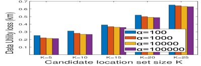
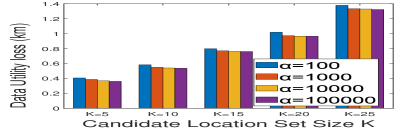
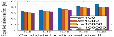
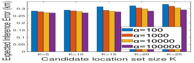
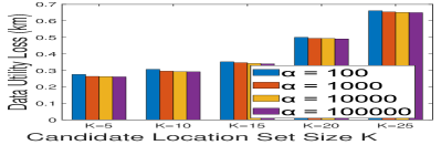
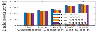
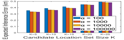
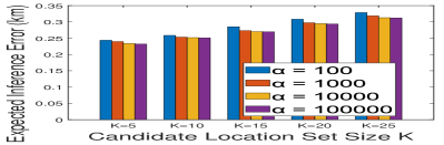
(1) The TransProtect parameters (candidate location set size) and (utility loss weight) impact the data utiltiy loss. We present the average data utility loss and the expected inference error of “Laplace+TransProtect” and “LP+TransProtect” given different and for the Rome and San Francisco datasets in Fig. 12(a)(b) and Fig. 12(a)(b), and Fig. 14(a)(b) and Fig. 14(a)(b), respectively. In addition, the expected utility loss and the expected inference error of the two methods with different values of and are shown in Table 4 and Table 5. The figures and tables show that the average data utility loss and expected inference error of “Laplace+TransProtect” and “LP+TransProtect” increases with an increase in . This is because a higher value of expands the candidate location set, providing a chance for locations with higher data utility loss to be selected.
In Fig. 12(a)(b), Fig. 12(a)(b), Fig. 14(a)(b) and Fig. 14(a)(b), we find that when increases, both data utility loss and expected inference error of “Laplace+ TransProtect” and “LP+TransProtect” decreases. This is because a higher value results in locations with lower data utility loss having a comparatively higher score than locations with higher probability scores (output by the Transformer encoder), making them more likely to be selected as candidate locations. Fig. 12(a)(b) and Fig. 14(a)(b) provides a visual example, illustrating that when , certain locations with higher data utility loss are included in the candidate location set. Conversely, when , almost all candidate locations can achieve low data utility loss. Fig. 12(a)(b) and Fig. 14(a)(b) also indicates that once , data utility loss plays a predominant role in candidate location selection in TransProtect, and further increases in do not significantly impact data utility loss (as observed when comparing data utility loss at and ).
In addition, Fig. 15(a)(b)(c) give illustrative examples to show how and impact the data utility loss. Fig. 15(a)(b) shows that when is increased from 10 to 15, more locations with higher data utility loss become part of the candidate location set. Fig. 15(a)(c) shows that when , some locations with higher utility loss are included in the candidate location set, while when , almost all the candidate locations can achieve low utility loss. The figure also indicates that when , utility loss already achieves the major role in candidate location selection in TransProtect, and further increasing won’t impact the utility loss significantly (by comparing the utility loss when ).
*(a)(b)(c) shows the heatmap of the data utility loss of the locations around a real location (marked by red).