Finite-momentum superconductivity in two-dimensional altermagnets
with a Rashba-type spin-orbit coupling

Abstract

We theoretically study the finite-momentum superconductivity in two-dimensional (2D) altermagnets with a Rashba-type spin-orbit coupling (RSOC). We show the phase diagrams obtained by solving the linearized gap equation. We consider two directions of the Néel vector of the 2D altermagnet: parallel to the $x$-$y$ plane (in-plane) and perpendicular to the $x$-$y$ plane (out-of-plane). For the in-plane Néel vector, we find two different finite-momentum $d_{x^{2}-y^{2}}$-wave superconducting states distinguished by a dominant pairing channel: the inter-band pairing or the intra-band pairing. Furthermore, it is shown that an asymmetric deformation of Fermi surfaces caused by spin-splitting effects due to the in-plane altermagnet and the RSOC stabilizes the finite-momentum superconductivity with a large band splitting. For the out-of-plane Néel vector, the finite-momentum superconductivity is found only in the inter-band pairing mechanism, which is in contrast to the in-plane case.

1 Introduction

The formation of Cooper pairs is a fundamental concept to understand distinctive properties of superconductors. In the conventional superconductors, the Cooper pair is formed by two electrons of the time reversal pair on the Fermi surface, and thus its center-of-mass momentum becomes zero. However, once a spin degeneracy of the energy dispersion is lifted by the breaking of the time reversal symmetry, finite-momentum superconductivity, that is, the Cooper pairs with a finite momentum $\bm{q}\neq\bm{0}$, can be stabilized. The finite-momentum superconductivity induced by a strong magnetic field or an intrinsic net magnetization is known as the Fulde–Ferrell–Larkin–Ovchinnikov (FFLO) state[1, 2, 3]. The LO state is characterized by two nonzero momenta $\pm\bm{q}$ and exhibits a amplitude modulation of the order parameter. On the other hand, the FF state chooses a single nonzero momentum $\bm{q}$ and exhibits a phase modulation of the order parameter.

In noncentrosymmetric systems, an asymmetric spin-orbit coupling such as a Rashba-type spin-orbit coupling (RSOC) can arise. There are a lot of studies on superconductors with a spin-orbit coupling [4, 5, 6, 7, 8, 9, 10, 11, 12, 13]. Especially, coupled with an in-plane magnetic field, the RSOC can make the FF state more stable than the LO state because the two momenta $\pm\bm{q}$ is no longer equivalent. In this context, the FF state is called the helical state [5, 6, 11, 12]. Because both of spatial inversion symmetry and time reversal symmetry are broken, nonreciprocal transports such as the superconducting diode effect (SDE) can be realized [14, 15, 16, 17, 18, 19, 20]. Since the helical superconducting state is believed to be a key to the SDE [17, 16, 15], a fundamental understanding of it is crucial for comprehending and controlling of nonreciprocal transport properties in superconductors.

Here, we focus on altermagnets as candidate materials for realization of the finite-momentum superconductivity. Altermagnetism is the newly discorvered magnetism which have a momentum-dependent spin-splitting of the energy band without net magnetization[21, 22, 23, 24, 25, 26, 27, 28, 29, 30]. As the influence of magnetism on superconductivity has been broadly studied in condensed matter physics [31, 32, 33], the interplay between the altermagnetic spin-splitting and the superconductivity has recently attractted much attention[34, 35, 36, 37, 38, 39, 40, 41, 42, 43, 44, 45, 46]. Especially, the finite-momentum superconductivity in altermagnets has been theoretically proposed and shows some intriguing features such as the field-induced superconductivity[37] and the zero-field FFLO state[37, 38, 40]. In addition, the SDE in altermagnets has been reported in several theoretical works[40, 47, 42]. However, the property of the finite-momentum superconductivity in the altermagnet with the RSOC has been limited [42]. It is necessary to understand the combined effect of the altermagnet and the RSOC when considering the application of altermagnets to the devices related to the SDE.

Motivated by these backgrounds, in this paper, we calculate the possibility of the $d$-wave finite-momentum superconductivity in a two-dimensional (2D) altermagnet, taking the effect of the RSOC into account. Two directions of the Néel vector, in-plane and out-of-plane, are considered. For the in-plane altermagnet, since the altermagnetic spin-splitting and the RSOC are coupled with each other, the Fermi surfaces are deformed into asymmetric shapes, and generate two different finite-momentum superconducting states characterized by a dominant pairing channel. Furthermore, we explain a stabilization mechanism of the finite-momentum superconductivity based on the shapes of the Fermi surfaces influenced by anisotropic spin-splitting. For the out-of-plane altermagnet, we find that the Bardeen–Cooper–Schrieffer (BCS) state is stable for the intra-band pairing and the finite-momentum superconductivity appears only for the inter-band pairing. The difference between the directions of the Néel vector originates from a qualitative change of the Fermi surfaces and spin textures.

2 Model and Method

We consider finite-momentum superconductivity possibly realized in metallic $d$-wave altermagnets with the RSOC. The normal-state Hamiltonian of this system is written as

$$\hat{H}_{0}= \sum_{\bm{k}}\sum_{\sigma\sigma^{\prime}}\hat{c}^{\dagger}_{\bm{k}\sigma}[H_{0}(\bm{k})]_{\sigma\sigma^{\prime}}\hat{c}_{\bm{k}\sigma^{\prime}},$$ (1)

where $c^{\dagger}_{\bm{k}\sigma}$ ($c_{\bm{k}\sigma}$) is the creation (annihilation) operator of an electron with spin $\sigma$ and momentum $\bm{k}$. The $2\times 2$ matrix $H_{0}(\bm{k})$ is given by

$$H_{0}(\bm{k})=\frac{k^{2}}{2m}-\mu+\bm{h}(\bm{k})\cdot\bm{\sigma},$$ (2)

where $m$ is the mass of an electron, $\mu$ is the chemical potential, and $\bm{\sigma}=(\sigma_{x},\sigma_{y},\sigma_{z})$ is the Pauli vector. In the last term, $\bm{h}(\bm{k})$ represents the momentum-dependent spin-splitting caused by the RSOC and the $d$-wave altermagnet, written as

$$\bm{h}(\bm{k})=\Delta_{\mathrm{so}}\hat{\bm{k}}\times\bm{e}_{z}+\Delta_{\mathrm{AM}}(\hat{k}_{x}^{2}-\hat{k}_{y}^{2})\bm{n},$$ (3)

where $\hat{\bm{k}}=\bm{k}/k_{\mathrm{F}}$ with $k_{\mathrm{F}}=\sqrt{2m\mu}$, $\Delta_{\mathrm{so}}$ and $\Delta_{\mathrm{AM}}$ are the strength of the RSOC and the $d$-wave altermagnetic spin-splitting, respectively. The Néel vector of the altermagnetism is denoted by $\bm{n}$, and in this paper, we consider both cases: $\bm{n}$ is parallel to the $x$-$y$ plane (the in-plane altermagnet), and $\bm{n}$ is along $z$-axis (the out-of-plane altermagnet). The eigenvalues of Eq. (2) can be written as

$$E_{\lambda}(\bm{k})=\xi_{k}+\lambda|\bm{h}(\bm{k})|,$$ (4)

where $\xi_{k}=k^{2}/2m-\mu$ and $\lambda=\pm$ denotes band indices.

Next, we introduce the following form of an attractive interaction for Cooper pair formations:

$$\hat{H}_{V}=\frac{1}{\Omega}\sum_{\bm{k}\bm{k}^{\prime}}\hat{c}^{\dagger}_{\bm{k}+\bm{q}/2\uparrow}\hat{c}^{\dagger}_{-\bm{k}+\bm{q}/2\downarrow}V(|\bm{k}-\bm{k}^{\prime}|)\hat{c}_{-\bm{k}^{\prime}+\bm{q}/2\downarrow}\hat{c}_{\bm{k}^{\prime}+\bm{q}/2\uparrow},$$ (5)

where $\bm{q}$ is the center-of-mass momentum of the Cooper pairs, $\Omega$ is the volume of the system and $V(|\bm{k}-\bm{k}^{\prime}|)$ is the Fourier component of the attractive interaction between two electrons.

We apply the mean-field approximation to Eq. (5) by defining the superconducting order parameter defined as

$$\Delta_{\sigma\sigma^{\prime}}(\bm{k},\bm{q})=-\frac{1}{\Omega}\sum_{\bm{k}^{\prime}}V(|\bm{k}-\bm{k}^{\prime}|)\expectationvalue{\hat{c}_{\bm{k}^{\prime}+\bm{q}/2\sigma}\hat{c}_{-\bm{k}^{\prime}+\bm{q}/2\sigma^{\prime}}}.$$ (6)

Then, the total Hamiltonian $\hat{H}_{0}+\hat{H}_{V}$ is reduced to

$$\hat{H}^{\mathrm{MF}} =\sum_{\bm{k}}\sum_{\sigma\sigma^{\prime}}\hat{c}^{\dagger}_{\bm{k}\sigma}[H_{0}(\bm{k})]_{\sigma\sigma^{\prime}}\hat{c}_{\bm{k}\sigma^{\prime}}$$ (7)

$$+\frac{1}{\Omega}\sum_{\bm{k}}\Delta_{\uparrow\downarrow}(\bm{k},\bm{q})\hat{c}^{\dagger}_{\bm{k}+\bm{q}/2\uparrow}\hat{c}^{\dagger}_{-\bm{k}+\bm{q}/2\downarrow}+\mathrm{H.c.}+\mathrm{const.}$$

We linearize the gap equation (6) by using the Gor’kov equation. The Green’s function and the anomalous Green’s function are defined as follows:

$$G_{\sigma\sigma^{\prime}}(\bm{k}_{+},\omega_{n}) \equiv-\int^{\beta}_{0}\mathrm{d}\tau\,e^{i\omega_{n}\tau}\expectationvalue{\hat{c}_{\bm{k}_{+}\sigma}(\tau)\hat{c}^{\dagger}_{\bm{k}_{+}\sigma^{\prime}}},$$ (8)

$$F_{\sigma\sigma^{\prime}}(\bm{k},\bm{q},\omega_{n}) \equiv-\int^{\beta}_{0}\mathrm{d}\tau\,e^{i\omega_{n}\tau}\expectationvalue{\hat{c}_{\bm{k}_{+}\sigma}(\tau)\hat{c}_{-\bm{k}_{-}\sigma^{\prime}}},$$ (9)

where $\bm{k}_{\pm}=\bm{k}\pm\bm{q}/2$, $\omega_{n}=\pi k_{\mathrm{B}}T(2n+1)$ is the Matsubara frequency, $\beta=1/k_{\mathrm{B}}T$ is the inverse temperature, and $\hat{c}_{\bm{k}\sigma}(\tau)=e^{\tau\hat{H}^{\mathrm{MF}}}\hat{c}_{\bm{k}\sigma}e^{-\tau\hat{H}^{\mathrm{MF}}}$. The Gor’kov equation can be derived as

$$[i\omega_{n}\check{I}-\check{H}_{\mathrm{BdG}}(\bm{k},\bm{q})]\check{G}(\bm{k},\bm{q};\omega_{n})=\check{I}$$ (10)

with

$$\check{H}_{\mathrm{BdG}}(\bm{k},\bm{q}) =\begin{pmatrix}H_{0}(\bm{k}_{+})&\Delta(\bm{k},\bm{q})\\ -\Delta^{*}(-\bm{k},\bm{q})&-H^{*}_{0}(-\bm{k}_{-})\end{pmatrix},$$ (11)

$$\check{G}(\bm{k},\bm{q};i\omega_{n}) =\begin{pmatrix}G(\bm{k}_{+},\omega_{n})&F(\bm{k},\bm{q},\omega_{n})\\ -F^{*}(-\bm{k},\bm{q},\omega_{n})&-G^{*}(-\bm{k}_{-},\omega_{n})\end{pmatrix},$$ (12)

where $\check{\cdot}$ describes a $4\times 4$ matrix, and $\check{I}$ denotes the $4\times 4$ unit matrix. The matrix elements of $2\times 2$ matrices $\Delta(\bm{k},\bm{q})$, $G(\bm{k}_{+},\omega_{n})$, and $F(\bm{k},\bm{q},\omega_{n})$ are given by Eq. (6), Eq. (8), and Eq. (9), respectively. Using the anomalous Green’s function, the gap equation is represented as

$$\Delta(\bm{k},\bm{q})=\frac{k_{\mathrm{B}}T}{\Omega}\sum_{\bm{k}^{\prime}}\sum_{n}V(|\bm{k}-\bm{k}^{\prime}|)F(\bm{k}^{\prime},\bm{q},\omega_{n}).$$ (13)

We consider the spin-singlet order parameter, and show the results for the $d$-wave superconducting order parameter in the main text. The phase diagram for the $s$-wave order parameter is shown in the Appendix. The spin-singlet order parameter $\Delta(\bm{k},\bm{q})$ and the attractive interaction $V(|\bm{k}-\bm{k}^{\prime}|)$ can be decomposed as

$$\Delta(\bm{k},\bm{q}) =\Delta(\bm{q})w_{\bm{k}}\,(i\sigma_{y}),$$ (14)

$$V(|\bm{k}-\bm{k}^{\prime}|) =-Vw_{\bm{k}}w_{\bm{k^{\prime}}},$$ (15)

where $V>0$ is a constant attractive strength. Here, $w_{\bm{k}}=~{}1$ for the $s$-wave order parameter, and $w_{\bm{k}}=\sqrt{2}\cos{2\phi}$ for the $d$-wave order parameter, where $\phi$ is an azimuthal angle in the $k_{x}$-$k_{y}$ plane. The node directions of the $w_{\bm{k}}$ is the same as those for the altermagnetic term in Eq. (3). From Eq. (10), $F(\bm{k},\bm{q},i\omega_{n})$ can be obtained perturbatively up to the first order of $\Delta(\bm{k},\bm{q})$. Substituting the perturbative solution of $F(\bm{k},\bm{q},i\omega_{n})$, Eqs. (14) and (15) into Eq. (13), we obtain the linearized gap equation

$$1=\frac{k_{\text{B}}TV}{2\Omega}\sum_{\bm{k}}\sum_{n}\Tr\sigma_{y}G_{0}(\bm{k}_{+},\omega_{n})\sigma_{y}G^{*}_{0}(-\bm{k}_{-},\omega_{n})w^{2}_{\bm{k}},$$ (16)

where $G_{0}(\bm{k})=(i\omega_{n}-H_{0}(\bm{k}))^{-1}$. By performing the summation over the Matsubara frequency, Eq. (16) can be rewritten as [11, 12]

$$1=\frac{V}{\Omega}\sum_{\bm{k}}\sum_{\lambda,p}\frac{|u_{p}|^{2}}{4E^{(s)}_{\lambda,p}}\frac{\sinh{\beta E^{(s)}_{\lambda,p}}}{\cosh{\beta E^{(s)}_{\lambda,p}}+\cosh{\beta E^{(a)}_{\lambda,p}}}w^{2}_{\bm{k}},$$ (17)

where $\lambda=\pm$, and $p=\mathrm{inter}$ or $\mathrm{intra}$. Here, we have defined $E^{(s)}_{\lambda,p}$ and $E^{(a)}_{\lambda,p}$ as

$$E^{(s)/(a)}_{\lambda,\mathrm{inter}} =\frac{E_{\lambda}(\bm{k}_{+})\pm E_{-\lambda}(-\bm{k}_{-})}{2}$$ (18)

$$E^{(s)/(a)}_{\lambda,\mathrm{intra}} =\frac{E_{\lambda}(\bm{k}_{+})\pm E_{\lambda}(-\bm{k}_{-})}{2},$$ (19)

and $|u_{\mathrm{inter/intra}}|^{2}$ as

$$|u_{\mathrm{inter/intra}}|^{2}=\frac{1\pm\cos{\theta}(\bm{k},\bm{q})}{2},$$ (20)

where $\theta(\bm{k},\bm{q})$ is the angle between $\bm{h}(\bm{k}_{+})$ and $\bm{h}(-\bm{k}_{-})$, that is,

$$\cos{\theta}(\bm{k},\bm{q})=\frac{\bm{h}(\bm{k}_{+})\cdot\bm{h}(-\bm{k}_{-})}{|\bm{h}(\bm{k}_{+})||\bm{h}(-\bm{k}_{-})|}.$$ (21)

Note that $|u_{\mathrm{inter}}|^{2}=1$ and $|u_{\mathrm{intra}}|^{2}=0$ ($|u_{\mathrm{inter}}|^{2}=0$ and $|u_{\mathrm{intra}}|^{2}=1$) for $\theta=0$ ($\theta=\pi$). The direction of $h(\bm{k})$ is the same as (opposite to) that of the electron spin on $\lambda=+$ ($-$) band at $\bm{k}$. Thus, the spin of the electron with $\bm{k}_{+}$ on one band is anti-parallel to that of the electron with $-\bm{k}_{-}$ on the other band for $\theta=0$ while on the same band for $\theta=\pi$.

Instead of directly solving the linerized gap equation (17), we introduce

$$K(\bm{q})=\frac{V}{\Omega}\sum_{\bm{k}}\sum_{\lambda,p}\frac{|u_{p}|^{2}}{4E^{(s)}_{\lambda,p}}\frac{\sinh{\beta E^{(s)}_{\lambda,p}}}{\cosh{\beta E^{(s)}_{\lambda,p}}+\cosh{\beta E^{(a)}_{\lambda,p}}}w^{2}_{\bm{k}}-1,$$ (22)

and investigate $K_{\max}=\max_{\bm{q}}K(\bm{q})=K(\bm{q}_{\max})$. Although we explicitly show only $\bm{q}$ as the argument of $K$, $K_{\max}$ as well as $K(\bm{q})$ depends on $\Delta_{\mathrm{so}}$, $\Delta_{\mathrm{AM}}$, and $T$. The other parameters such as $\mu$ are fixed as specified below. The center-of-mass momentum which maximizes $K(\bm{q})$, $\bm{q}_{\max}$, is the momentum which is most promising to be realized. However, far from the phase boundary, the optimal momentum should be determined by solving the gap equation self-consistently. The linearized gap equation can be represented as $K_{\max}=0$ for the above-mentioned parameters. Particularly, we define $\Delta_{\mathrm{AM,c}}$ such that $K_{\max}=0$ for given $\Delta_{\mathrm{so}}$ and $T$. We also define $\bm{q}_{\max,\mathrm{c}}$ which maximizes $K(\bm{q})$ for $\Delta_{\mathrm{AM,c}}$. As seen from the summation over $p$ in Eq. (22), there are two contributions: one from the inter-band pairing and the other from the intra-band pairing. Therefore, the dominant pairing channel can be estimated by comparing the weights of these two contributions.

3 Results

3.1 In-plane altermanget

We first show the phase diagram for the in-plane altermagnet in the $\Delta_{\mathrm{so}}$-$\Delta_{\mathrm{AM}}$ plane at a fixed temperature $T=0.01T_{\mathrm{c}}$ in Fig. 1(a). We set $\bm{n}=\hat{\bm{y}}$ in Eq. (3) for simplicity. As units of the temperature, the energies, and the momentum of Cooper pairs, we introduce the following quantities for $\Delta_{\mathrm{so}}=\Delta_{\mathrm{AM}}=0$, respectively: $T_{\mathrm{c}}$, $\Delta_{0}$, and $q_{0}$, where $T_{\mathrm{c}}$ is the critical temperature, $\Delta_{0}=(\pi/e^{\gamma})k_{\mathrm{B}}T_{\mathrm{c}}$ is the $s$-wave superconducting gap at $T=0$, and $q_{0}=\Delta_{0}/\varv_{\mathrm{\mathrm{F}}}$ with the Fermi velocity $\varv_{\mathrm{F}}=\sqrt{2\mu/m}$ corresponds to the inverse coherence-length. We set $\mu=50\Delta_{0}$ unless mentioned otherwise. The blue line in Fig. 1(a), along which $K_{\max}=0$, accounts for the second-order transition between the superconducting state and the normal state. Below (Above) this line, $K_{\max}>0$ ($K_{\max}<0$), and thus the superconducting (normal) state is expected. The phase diagram consists of two superconducting states, both of which are the finite-momentum superconductivity. They are separated by the red line in Fig. 1(a), across which $\bm{q}_{\max}$ changes discontinuously. Thus, a first-order transition is expected, although this is based on the linearized analysis and requires the self-consistent calculation for further studies. The first-order transition line starts from the tricritical point $\mathsf{T}$ at $(\Delta_{\mathrm{so}}^{*}/\Delta_{0},\Delta_{\mathrm{AM}}^{*}/\Delta_{0})\approx(1.38,1.51)$, which is on the second-order phase transition line between the two superconducting states and the normal state. One can see that the first-order transition takes place when $\Delta_{\mathrm{so}}$ and $\Delta_{\mathrm{AM}}$ are comparable. Along the green arrow ($\Delta_{\mathrm{AM}}=1.15\Delta_{0}$) indicated in Fig. 1(a), we show the changes in the Cooper pair momentum $\bm{q}_{\max}$ and the pairing structure in Figs. 2(a) and 2(b), respectively. As seen from Fig. 2(a), the $y$-component of $\bm{q}_{\max}$ is zero in this range of $\Delta_{\mathrm{so}}$, and the $x$-component changes its sign and magnitude when across the red line at $\Delta_{\mathrm{so}}/\Delta_{0}\sim 1.05$. Note that, when $\Delta_{\mathrm{so}}$ is nonzero, $K(\bm{q})$ is not symmetric under the sign reversal of $q_{x}$ for $\bm{n}=\hat{\bm{y}}$ as shown in the inset of Fig. 2(a). In Fig. 2(b), the contribution to $K(\bm{q})$ from each pairing channel is shown. Corresponding to the discontinuous change in $\bm{q}_{\max}$, one can see that the dominant pairing of the Cooper pairs also switches from the inter-band pairing to the intra-band pairing with increasing $\Delta_{\mathrm{so}}$. These details indicate that two different superconducting states correspond to the different pairing channels, accompanied by the discontinuous change of the optimal momentum of the Cooper pairs [11, 12].

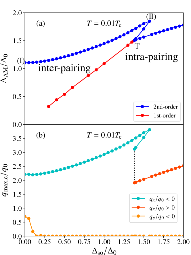
Figure 1: (a) Phase diagram for the in-plane altermagnet in the $\Delta_{\mathrm{so}}$-$\Delta_{\mathrm{AM}}$ plane at $T=0.01T_{\mathrm{c}}$. “Inter-pairing” (“intra-pairing”) denotes the superconducting states mainly from the inter-band pairing (the intra-band pairing). The blue line corresponds to $\Delta_{\mathrm{AM,c}}$ for each $\Delta_{\mathrm{so}}$, which accounts for the phase boundary between the superconducting state and the normal state. The red line denotes the first-order transition line between the inter-band pairing and the intra-band pairing. (b) $\bm{q}_{\mathrm{max,c}}$ along the blue line in (a). The cyan (red) line shows negative (positive) $q_{x}$, $x$-component of $\bm{q}_{\mathrm{max,c}}$, and the orange line shows $q_{y}$. The dotted line represents a discontinuous change of $\bm{q}_{\mathrm{max,c}}$ at the tricritical point $\mathsf{T}$ in (a).

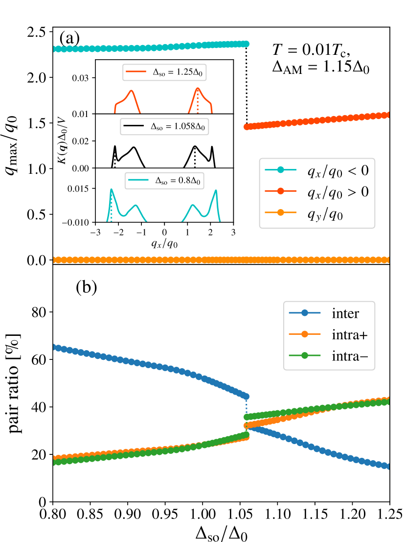
Figure 2: (a) $\bm{q}_{\mathrm{max}}$ and (b) the contributions to $K(\bm{q})$ from each pairing channel along the green arrow drawn in Fig. 1(a). $\Delta_{\mathrm{AM}}$ is fixed to $1.15\Delta_{0}$, and $\Delta_{\mathrm{so}}$ changes from $0.8\Delta_{0}$ to $1.25\Delta_{0}$. The inset in (a) shows the $q_{x}$ dependence of $K(\bm{q})$ for three $\Delta_{\mathrm{so}}$’s with $q_{y}=0$. The dotted lines in each panel in the inset denote corresponding $\bm{q}_{\mathrm{max}}$. “Intra$+$” (“intra$-$”) in (b) represents the contributions from the intra-band pairing which consists of two electrons on the $\lambda=+$ ($-$) band.

For the in-plane altermagnet, the energy dispersion $E^{\mathrm{in}}_{\lambda}(\bm{k})$ is given as

$$E^{\mathrm{in}}_{\lambda}(\bm{k})=\xi_{k}+\lambda\sqrt{\quantity[-\Delta_{\mathrm{so}}\hat{k}_{x}+\Delta_{\mathrm{AM}}\quantity(\hat{k}^{2}_{x}-\hat{k}^{2}_{y})]^{2}+\Delta_{\mathrm{so}}^{2}\hat{k}_{y}^{2}},$$ (23)

and the expectation value of the spin direction at momentum $\bm{k}$ on band $\lambda$ is

$$\expectationvalue{\bm{\sigma}^{\mathrm{in}}_{\lambda}}=\frac{\lambda}{|\bm{h}(\bm{k})|}\quantity(\Delta_{\mathrm{so}}\hat{k}_{y},-\Delta_{\mathrm{so}}\hat{k}_{x}+\Delta_{\mathrm{AM}}(\hat{k}^{2}_{x}-\hat{k}^{2}_{y}),0)$$ (24)

The Fermi surfaces of the normal states calculated from $E^{\mathrm{in}}_{\lambda}(\bm{k})=0$ for some parameter sets are shown in Fig. 3. The orange (green) arrows show the in-plane spin polarization on a $\lambda=+(-)$ band. For $\Delta_{\mathrm{so}}=0$ [Fig. 3(a)], there is ambiguity in the definition of the bands because the two bands are degenerated at the $\bm{k}$ points along $k_{x}=\pm k_{y}$, where the altermagnetic splitting is absent. In our definition, the direction of the electron spin on each band is not constant but alternates every $90^{\circ}$ rotation for continuity to the case with nonzero $\Delta_{\mathrm{so}}$. For $s$-wave superconductors, the conventional BCS-pairing can be formed by using electrons at degenerate points. However, such pairings are prohibited in the $d_{x^{2}-y^{2}}$-wave superconductors because the $d_{x^{2}-y^{2}}$-wave superconducting order parameter have the same node-directions as those for the altermagnetic spin-splitting. Other than the node directions, an up-spin electron at $(k_{x},k_{y})$ on one band cannot find a down-spin electron at $(-k_{x},-k_{y})$ on the same band, but can find it at $(-k_{x}+q_{x},-k_{y}+q_{y})$ on the other band. This mechanism makes the finite-momentum inter-band pairing stable [37, 38, 40]. For $\Delta_{\mathrm{so}}\neq 0$, the degeneracies are lifted and the two Fermi surfaces are shifted in the opposite $k_{x}$-directions. In addition, since $\expectationvalue{\sigma_{x}}$ in Eq. (24) becomes finite, the spin texture in momentum space appears. For $\Delta_{\mathrm{so}}<\Delta_{\mathrm{AM}}$ [Fig. 3(b)], the altermagnetic spin configuration is dominant, and therefore, the inter-band pairing scenario is still applicable. In the case of $\Delta_{\mathrm{so}}>\Delta_{\mathrm{AM}}$ [Fig. 3(c)], the spin directions are dominated by the RSOC, and thus the intra-band pairing becomes more stable than the inter-band pairing.

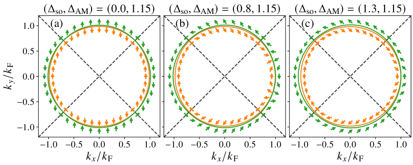
Figure 3: The Fermi surfaces ($E^{\mathrm{in}}_{\lambda}(\bm{k})=0$) and the spin texture for (a) $\Delta_{\mathrm{so}}=0$, (b) $\Delta_{\mathrm{AM}}>\Delta_{\mathrm{so}}$ and (c)$\Delta_{\mathrm{AM}}<\Delta_{\mathrm{so}}$. Two bands are distinguished by using different colors. In each panel, the orange (green) represents $\lambda=+(-)$ band. Arrows indicate the direction of the in-plane spin polarization. The dotted lines correspond to the directions along which altermagnetic spin-splitting is absent.

We make a remark on the $d$-wave superconductors in the altermagnet without the RSOC which is studied for $T=0$ in the previous work[37]. We show the $T$-$\Delta_{\mathrm{AM}}$ phase diagram for finite temperatures in Fig. 4 and discuss the temperature dependence of $\bm{q}_{\max,\mathrm{c}}$. In Fig.4, the blue solid circles ($T\lesssim 0.55T_{\mathrm{c}}$) account for the finite-momentum superconductivity (FF-state), while the open circles do the conventional BCS pairing, along the phase boundary. Focusing on the variation of $\bm{q}_{\mathrm{max,c}}$, one can see that the orientation of $\bm{q}_{\mathrm{max,c}}$ depends on the temperatures, and it gradually changes from $45^{\circ}$ to small angles with temperature decreasing. To investigate details, we show phase diagrams for different orientations of the momentum in Fig. 5. For temperatures above $T^{*}\approx 0.1T_{\mathrm{c}}$, the finite momentum-superconductivity whose $\bm{q}_{\mathrm{max,c}}$ is along $45^{\circ}$ has the largest $\Delta_{\mathrm{AM}}$. As temperature decreases, the most stable orientation continuously changes from $45^{\circ}$ to smaller angles. These results at low temperatures are consistent with the previous work[37]. We additionally note that the similar temperature dependence of $\bm{q}_{\mathrm{max,c}}$ is reported in a 2D $d$-wave superconductor with a uniform magnetic field[48].

Figure 1(a) shows that only $q_{x}$ remains finite while $q_{y}$ is zero when both effects of the RSOC and the altermagnetic spin-splitting is finite. The phase diagrams with $\Delta_{\mathrm{so}}=\Delta_{0}$ for several different orientations of $\bm{q}_{\mathrm{max,c}}$ are shown in Fig. 6(a), where the state with the momentum along the $x$-direction is confirmed to be the most stable particular in the low temperature region. One can see from Fig. 6(b) that $\bm{q}_{\mathrm{max,c}}$ for $\alpha=45^{\circ}$, $90^{\circ}$, and $135^{\circ}$ becomes zero or much smaller than those for $\alpha=0^{\circ}$ and $180^{\circ}$, which means that the pairing states are similar to the BCS state. Hence, the upturn behavior in the low temperature region cannot be observed for those angles [Fig. 6(a)]. The slight difference of $\Delta_{\mathrm{AM,c}}$ and $q_{\mathrm{max,c}}$ between $\alpha=0^{\circ}$ and $180^{\circ}$ represent that $\bm{q}$ and $-\bm{q}$ are no longer equivalent, as mentioned above. The previous studies have shown that in a system with the RSOC and the in-plane magnetic field, the finite-momentum superconductivity whose momentum is perpendicular to the magnetic field gets stable[5, 6]. Therefore, our result is consistent with the situation of the helical state.

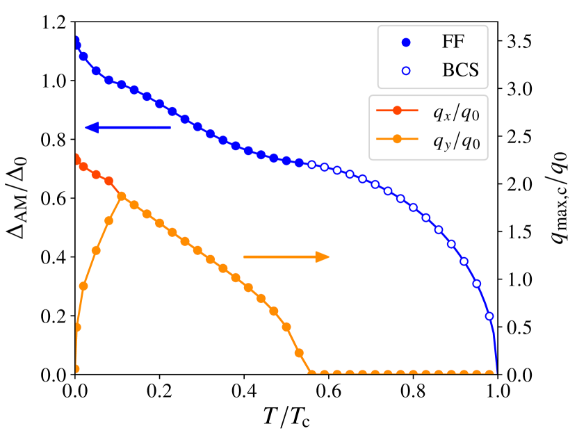
Figure 4: The phase diagram in the $T$-$\Delta_{\mathrm{AM}}$ plane and the temperature dependence of $\bm{q}_{\mathrm{max,c}}$ without the RSOC. The blue solid (open) circles account for the superconducting state whose momentum is finite (zero).

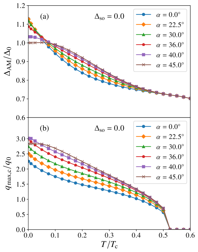
Figure 5: (a) The phase diagram in the $T$-$\Delta_{\mathrm{AM}}$ plane and (b) $\bm{q}_{\mathrm{max,c}}$ for several fixed orientations with $\Delta_{\mathrm{so}}=0$. The orientation of $\bm{q}_{\mathrm{max,c}}$ is denoted by $\alpha=\tan^{-1}(q_{y}/q_{x})$.

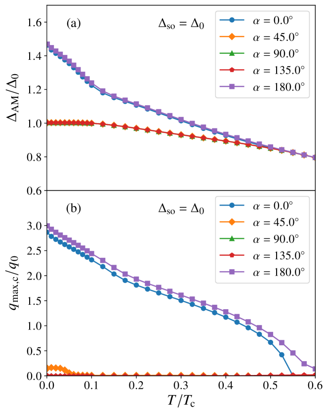
Figure 6: (a) The phase diagrams in the $T$-$\Delta_{\mathrm{AM}}$ plane and (b) $\bm{q}_{\mathrm{max,c}}$ for several fixed orientations ($\Delta_{\mathrm{so}}=\Delta_{0}$). The definition of $\alpha$ is the same as that in Fig. 5.

The upturn of the second-order transition line in the inter-band pairing region and the emergence of the reentrant region implies the finite-momentum superconductivity is stabilized at the larger $\Delta_{\mathrm{so}}$ and $\Delta_{\mathrm{AM}}$. The mechanism of the stabilization can be interpreted from the nesting condition for the FFLO state[49]. It has been reported that the enhancement of the critical field can be occurred when the two Fermi surfaces (FSs) $E_{\uparrow}(\bm{k}+\nobreak\bm{q}/2)=0$ and $E_{\downarrow}(-\bm{k}+\bm{q}/2)=0$ have a good fit. To check the nesting structure for the present system, Figs. 7(a) and 7(b) exhibit the two FSs. The green (orange) solid line represents $k^{\lambda=-}_{0}(\phi)$ [$k^{\lambda=+}_{0}(\phi+\pi)$,], where $k^{\lambda}_{0}(\phi)$ is the radial length of the FS as a function of an azimuthal angle $\phi$ and defined as

$$E^{\mathrm{in}}_{\lambda}\quantity(k^{\lambda}_{0}(\phi)\cos{\phi}+q_{x}/2,\,k^{\lambda}_{0}(\phi)\sin{\phi}+q_{y}/2)=0.$$ (25)

The intensity of the integrand of $K(\bm{q})$ at given parameters is also shown with color map. We choose two sets of parameters, (I) $(\Delta_{\mathrm{so}},\Delta_{\mathrm{AM}},q_{x},q_{y})\approx(0.0,1.10,-2.22,-0.711)$ for panel (a), and (II) $(\Delta_{\mathrm{so}},\Delta_{\mathrm{AM}},q_{x},q_{y})\approx(1.57,1.85,-3.81,0.0)$ for panel (b), which are also indicated in Figs. 1(a) and 1(b) by (I) and (II), respectively. As can be seen from the color map, the intensity of the integrand is enhanced when the two FSs cross or touch with each other in the area other than the nodes of the $d$-wave superconducting order parameter. By comparing Figs. 7(a) and 7(b), one can see the two FSs in Fig. 7(b) have a better fit around $\phi=\pi$. To evaluate how the two FSs touch with each other, we introduce $\Delta k_{0}(\phi)$, the difference of two radii involved in the formation of Cooper pairs, as $\Delta k_{0}(\phi)=k^{-}_{0}(\phi)-k^{+}_{0}(\phi+\pi)$. Figure 7(c) shows the values of the first derivative $\Delta k^{\prime}_{0}(\phi^{*})$, and the second derivative $\Delta k^{\prime\prime}_{0}(\phi^{*})$ at the intersection point $\phi^{*}$ of the two FSs, $\Delta k_{0}(\phi^{*})=0$, around $\phi=\pi$, for the parameter sets along the phase boundary of the inter-band pairing shown in Fig. 1(a). Note that nonzero $\Delta k^{\prime}_{0}(\phi^{*})$ accounts for the crossing of $k_{0}^{-}(\phi)$ and $k_{0}^{+}(\phi+\pi)$ at $\phi=\phi^{*}$. One can see that as $\Delta_{\mathrm{so}}$ increases, $|\Delta k^{\prime}_{0}(\phi^{*})|$ goes to zero and the two FSs touch at $\phi=\phi^{*}$. At the same time, $|\Delta k^{\prime\prime}_{0}(\phi^{*})|$ also goes to zero. By focusing on each second derivative $k_{0}^{\lambda\prime\prime}$ shown in the inset of Fig. 7(c), one can see that ${k^{+}_{0}}^{\prime\prime}(\phi+\pi)$ exhibits the sign change at $\Delta_{\mathrm{so}}\sim\Delta_{0}$, and the two FSs have the same curvature, that is, the better fit of the FSs is realized, as shown in Fig. 7(b). Therefore, when the altermagnetic spin-splitting is comparable with that of the RSOC, the finite-momentum superconductivity is stabilized via the deformation of the FSs.

Figure 7: (a) (b) Two FSs $k^{-}_{0}(\phi)$ (green solid line) and $k^{+}_{0}(\phi+\pi)$ (orange solid line). The intensity of the integrand of $K(\bm{q})$ is also shown with color map. The parameter sets for each figure are explained in the main text. The arrows represent orientations of electron spins in the $k_{x}$-$k_{y}$ plane. (c) The values of the first derivative $\Delta k^{\prime}_{0}(\phi^{*})$, and the second derivative $\Delta k^{\prime\prime}_{0}(\phi^{*})$ at the intersection point $\phi^{*}$ around $\pi$. The inset shows the second derivatives ${k^{-}_{0}}^{\prime\prime}(\phi^{*})$ and ${k^{+}_{0}}^{\prime\prime}(\phi^{*}+\pi)$. (d) The schematic illustration showing the definition of $k^{\lambda}_{0}(\phi)$ and $\phi$. The orange circle is the FS calculated from $E_{\lambda}(\bm{k}+\bm{q}/2)=0$.

3.2 Out-of-plane altermagnet

Figure 8 shows the $\Delta_{\mathrm{so}}$-$\Delta_{\mathrm{AM}}$ phase diagram at $T=0.01T_{\mathrm{c}}$ for the out-of-plane altermagnet which is described by $\bm{n}=\hat{\bm{z}}$ in Eq. (3). Note that $K(\bm{q})$ is symmetric under the sign reversal of $\bm{q}$ in the out-of-plane case, but we consider the single-$\bm{q}$ finite-momentum superconductivity, which corresponds to the FF state. The phase diagram also consists of the inter-band pairing superconductivity (the left side of the red line) and the intra-band pairing superconductivity (the right side of the red line). The Cooper-pair momentum is finite only for the inter-band pairing, and the BCS-pairing is stable for the intra-band pairing, in contrast to the case of the in-plane Néel vector. Moreover, the tricritical point $\mathsf{T}$ in the out-of-plane case is $(\Delta_{\mathrm{so}}^{*}/\Delta_{0},\Delta_{\mathrm{AM}}^{*}/\Delta_{0})\approx(0.32,1.08)$, and it is shifted to the lower $\Delta_{\mathrm{so}}$ side compared with the one in the in-plane case as discussed later. Consequently, compared to the in-plane altermagnet, the finite-momentum superconductivity is realized in a narrow region of the phase diagram.

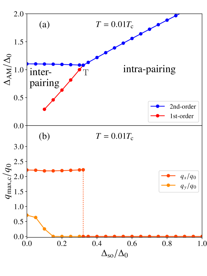
Figure 8: (a) The phase diagram of the out-of-plane altermagnet in the $\Delta_{\mathrm{so}}-\Delta_{\mathrm{AM}}$ plane. (b) $\bm{q}_{\mathrm{max,c}}$ along the second-order transition line in (a). Dotted line represents an abrupt change of $\bm{q}_{\mathrm{max,c}}$ at the tricritical point. Definitions of the lines are the same as those in Fig. 1.

The energy dispersion in the out-of-plane altermagnet can be obtained from Eq. (4) as

$$E^{\mathrm{out}}_{\lambda}(\bm{k})=\xi_{k}+\lambda\sqrt{\Delta_{\mathrm{so}}^{2}\hat{k}^{2}+\Delta_{\mathrm{AM}}^{2}(\hat{k}_{x}^{2}-\hat{k}_{y}^{2})^{2}}.$$ (26)

The expectation value of the electron spin at momentum $\bm{k}$ on band $\lambda$ is given by

$$\expectationvalue{\bm{\sigma}^{\mathrm{out}}_{\lambda}}=\frac{\lambda}{|\bm{h}(\bm{k})|}\quantity(\Delta_{\mathrm{so}}\hat{k}_{y},-\Delta_{\mathrm{so}}\hat{k}_{x},\Delta_{\mathrm{AM}}(\hat{k}^{2}_{x}-\hat{k}^{2}_{y})).$$ (27)

The Fermi surfaces calculated from $E^{\mathrm{out}}_{\lambda}(\bm{k})=0$ and the corresponding spin textures are shown in Fig. 9. In the in-plane altermagnet, the RSOC and the in-plane altermagnetic spin-splitting are coupled with each other. On the other hand, the RSOC and the altermagnetic spin-splitting are independent in the out-of-plane altermagnet in the following senses: as for the shape of the FS, the distortion and the shift of the FSs found in the in-plane altermagnet are absent in the out-of-plane altermagnet. As for the spin texture, while the RSOC affects the in-plane spin polarization, the altermagnetic effect affects the out-of-plane spin polarization. When the RSOC is zero, the spins have no in-plane components [Fig. 9(a)] and the finite-momentum inter-band pairing caused by the altermagnetic spin-splitting is realized. This scenario is the same as that of the in-plane altermagnet without the RSOC. However, when the RSOC is nonzero, the in-plane components of electron spins become finite. The in-plane component of the spin at $\bm{k}$ on one band is always antiparallel to that at $-\bm{k}$ on the same band, as seen from Eq. (27). In this intra-band pairing mechanism, the finite-momentum Cooper pairing is not favorable because there is no asymmetric distorsion or shift of the FSs. As a result, for larger values of $\Delta_{\mathrm{so}}$, the BCS pairing is stable by the intra-band pairing, the switching value of $\Delta_{\mathrm{so}}$ between the inter- and intra-band mechanisms is small compared with the in-plane altermagnetic case. This is because almost all the region of the FSs other than the nodal directions of the $d$-wave superconducting order parameter can contribute to the BCS superconductivity, in contrast to the case of the finite-momentum superconductivity as demonstrated in the left panels of Fig. 7. In other words, the finite-momentum superconductivity by the inter-band pairing can survive as long as $\Delta_{\mathrm{so}}$ is small, but once $\Delta_{\mathrm{so}}$ becomes large, the intra-band pairing with zero momentum can overcome the inter-band pairing. This is the main physical reason why the shrink of the inter-band pairing reaion and the intra-band pairing induces the BCS-pairing.

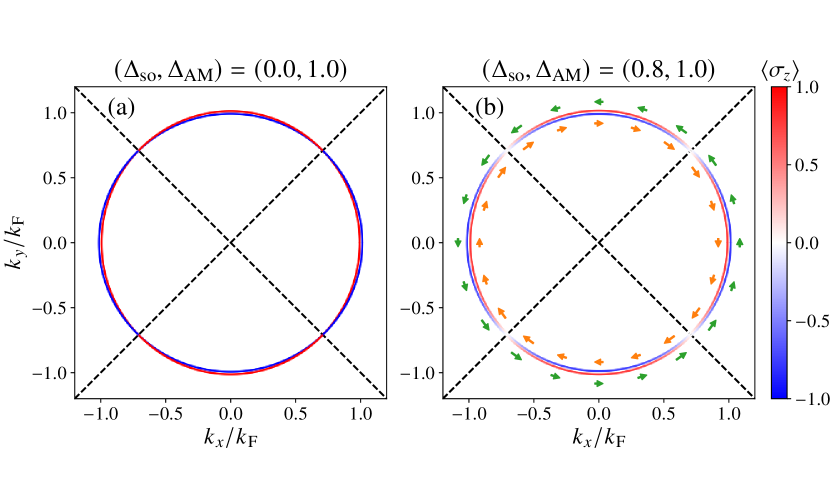
Figure 9: The Fermi surfaces and the spin texture for (a) $\Delta_{\mathrm{so}}=0$ case and (b) $\Delta_{\mathrm{so}}\neq 0$ case. The color of Fermi surfaces indicates the magnitude of $\expectationvalue{\sigma_{z}}$, the out-of-plane spin polarization. Color arrows indicate the direction of the in-plane spin polarization. Along the dotted lines, the altermagnetic spin-splitting is zero.

4 Conclusion

In this paper, we have investigated the possibility of the finite-momentum superconductivity in the two dimensional $d$-wave altermagnet with the RSOC, solving the linearized gap equation, and revealed two superconducting states in terms of whether the dominant pairing mechanism is the inter-band or inra-band pairing, dependeing on the strength of the altermagnetic spin-splitting $\Delta_{\mathrm{AM}}$ and the RSOC $\Delta_{\mathrm{so}}$. When the Néel vector of the altermagnetism is in the in-plane, both of the superconductivity favor the finite-momentum states, while the finite-momentum state is possible only for the inter-band pairing superconductivity in the case of the out-of-plane Néel vector. The origin of the difference between the in-plane and the out-of-plane altermagnet is explained by the appearance/absence of the asymmetric distorsion and the shift in the Fermi surface. In the case of the in-plane altermagnet, we have also clarified the expansion of the superconducting region in the phase diagram for $\Delta_{\mathrm{so}}\sim\Delta_{\mathrm{AM}}$, because of the nesting structure of the two Fermi surfaces contributing the inter-band superconductivity. The transition between these two superconducting states inside the ordered phase is expected to be discontinuous, but the self-consistent calculation is necessary for further studies.

Although we have only dealt with the spin-singlet superconducting order parameter, in general the spin-singlet and the spin-triplet superconductivity can be mixed in noncentrosymmetric systems. Therefore, it would be worthwhile to study parity-mixed finite-momentum superconducting states in altermagnets in the context of the topological superconductivity[34, 45, 46, 41]. In addition, the efficiency and the sign of the SDE are also important issues for applications of altermagnets. The sign change of the SDE has been reported when a phase transition of the superconductivity takes place [17, 18, 47]. Therefore, the influence on the SDE at the first-order transition discussed in the main text is one of the problems to be addressed in the future.

This work was supported by JSPS KAKENHI Grant Nos. JP24K17000 and JP23K22492.

Appendix A Phase diagram for $s$-wave order parameter

In this Appendix, we show the results for $s$-wave superconducting order parameter, as a comparison with the $d$-wave one discussed in the main text. Figure 10 shows the phase diagram in the case of the in-plane altermagnet. In Fig. 10, the first-order transition cannot be found in the $\Delta_{\mathrm{so}}$-$\Delta_{\mathrm{AM}}$ plane. In addition, the magnitude of $\bm{q}_{\mathrm{max,c}}$ in a weak $\Delta_{\mathrm{so}}$ region is smaller than that of $d$-wave superconductivity in the main text. When the RSOC is absent, the Fermi surfaces have the degenerate points along $k_{x}=\pm k_{y}$ as shown in Fig. 3(a). Even in the case of the in-place altermagnet, the BCS pairing at the degenerate points can be realized because the $s$-wave superconducting order parameter has the uniform amplitude along the Fermi surface, in contrast to the case of the $d$-wave superconductors. (The $d$-wave superconductors do not have the condensation energy without the Cooper pair momentum because of their node structure at the degenerate points[37].) As the strength of the RSOC gets larger, the $\Delta_{\mathrm{AM,c}}$ and the magnitude of $\bm{q}_{\mathrm{max,c}}$ also gets larger. It seems that finite-momentum superconductivity is realized in a wide range of parameters. However, this finite-momentum state is competed by the BCS pairing state even in the nonzero $\Delta_{\mathrm{so}}$, because the BCS pairing in the intra-bands can be formed along $k_{x}=\pm k_{y}$ lines though the degeneracy is lifted by the RSOC. Thus, the superconducting state far from the second-order transition line should be carefully studied by the self-consisitent calculation.

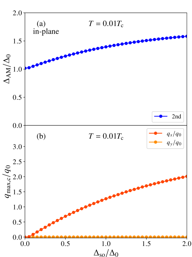
Figure 10: (a) The phase diagram in the $T$-$\Delta_{\mathrm{AM}}$ plane for $s$-wave superconductors in the in-plane altermagnet. (b) $\bm{q}_{\mathrm{max,c}}$ along the phase boundary in (a). Definitions of the lines are the same as those in Fig. 1.

References

- [1] P. Fulde and R. A. Ferrell: Phys. Rev. 135 (1964) A550.
- [2] A. I. Larkin and Y. N. Ovchinnikov: Zh. Eksperim. i Teor. Fiz. 47 (1964).
- [3] Y. Matsuda and H. Shimahara: J. Phys. Soc. Jpn. 76 (2007) 051005.
- [4] V. Barzykin and L. P. Gor’kov: Phys. Rev. Lett. 89 (2002) 227002.
- [5] R. P. Kaur, D. F. Agterberg, and M. Sigrist: Phys. Rev. Lett. 94 (2005) 137002.
- [6] D. F. Agterberg and R. P. Kaur: Phys. Rev. B 75 (2007) 064511.
- [7] O. Dimitrova and M. V. Feigel’man: Phys. Rev. B 76 (2007) 014522.
- [8] Y. Yanase and M. Sigrist: J. Phys. Soc. Jpn. 77 (2008) 342–344.
- [9] K. V. Samokhin: Phys. Rev. B 78 (2008) 224520.
- [10] K. Michaeli, A. C. Potter, and P. A. Lee: Phys. Rev. Lett. 108 (2012) 117003.
- [11] G. Zwicknagl, S. Jahns, and P. Fulde: J. Phys. Soc. Jpn. 86 (2017) 083701.
- [12] N. F. Q. Yuan and L. Fu: Proc. Natl. Acad. Sci. 118 (2021) e2019063118.
- [13] K. Aoyama: Phys. Rev. B 109 (2024) 024516.
- [14] N. Nagaosa and Y. Yanase: Annu. Rev. Condens. Matter Phys. 15 (2024) 63–83.
- [15] N. F. Q. Yuan and L. Fu: Proc. Natl. Acad. Sci. 119 (2022) e2119548119.
- [16] J. J. He, Y. Tanaka, and N. Nagaosa: New J. Phys. 24 (2022) 053014.
- [17] A. Daido, Y. Ikeda, and Y. Yanase: Phys. Rev. Lett. 128 (2022) 037001.
- [18] A. Daido and Y. Yanase: Phys. Rev. B 106 (2022) 205206.
- [19] S. Banerjee and M. S. Scheurer: Phys. Rev. Lett. 132 (2024) 046003.
- [20] J. Hasan, D. Shaffer, M. Khodas, and A. Levchenko: Phys. Rev. B 110 (2024) 024508.
- [21] K.-H. Ahn, A. Hariki, K.-W. Lee, and J. Kuneš: Phys. Rev. B 99 (2019) 184432.
- [22] S. Hayami, Y. Yanagi, and H. Kusunose: J. Phys. Soc. Jpn. 88 (2019) 123702.
- [23] L. Šmejkal, R. González-Hernández, T. Jungwirth, and J. Sinova: Sci. Adv. 6 (2020) eaaz8809.
- [24] L.-D. Yuan, Z. Wang, J.-W. Luo, E. I. Rashba, and A. Zunger: Phys. Rev. B 102 (2020) 014422.
- [25] M. Naka, S. Hayami, H. Kusunose, Y. Yanagi, Y. Motome, and H. Seo: Phys. Rev. B 102 (2020) 075112.
- [26] S. Hayami, Y. Yanagi, and H. Kusunose: Phys. Rev. B 102 (2020) 144441.
- [27] L. Šmejkal, J. Sinova, and T. Jungwirth: Phys. Rev. X 12 (2022) 031042.
- [28] L. Šmejkal, J. Sinova, and T. Jungwirth: Phys. Rev. X 12 (2022) 040501.
- [29] P. A. McClarty and J. G. Rau: Phys. Rev. Lett. 132 (2024) 176702.
- [30] M. Naka, S. Hayami, H. Kusunose, Y. Yanagi, Y. Motome, and H. Seo: Nat. Commun. 10 (2019) 4305.
- [31] D. J. Scalapino: Rev. Mod. Phys. 84 (2012) 1383.
- [32] E. Fradkin, S. A. Kivelson, and J. M. Tranquada: Rev. Mod. Phys. 87 (2015) 457–482.
- [33] D. Aoki, K. Ishida, and J. Flouquet: J. Phys. Soc. Jpn. 88 (2019) 022001.
- [34] D. Zhu, Z.-Y. Zhuang, Z. Wu, and Z. Yan: Phys. Rev. B 108 (2023) 184505.
- [35] B. Brekke, A. Brataas, and A. Sudbø: Phys. Rev. B 108 (2023) 224421.
- [36] A. A. Zyuzin: Phys. Rev. B 109 (2024) L220505.
- [37] D. Chakraborty and A. M. Black-Schaffer: Phys. Rev. B 110 (2024) L060508.
- [38] S. Sumita, M. Naka, and H. Seo: Phys. Rev. Res. 5 (2023) 043171.
- [39] S.-B. Zhang, L.-H. Hu, and T. Neupert: Nat. Commun. 15 (2024) 1801.
- [40] G. Sim and J. Knolle: arXiv:2407.01513 (2024).
- [41] S. Hong, M. J. Park, and K.-M. Kim: arXiv:2407.02059 (2024).
- [42] S. Banerjee and M. S. Scheurer: Phys. Rev. B 110 (2024) 024503.
- [43] A. Bose, S. Vadnais, and A. Paramekanti: arXiv:2403.17050 (2024).
- [44] H. G. Giil and J. Linder: Phys. Rev. B 109 (2024) 134511.
- [45] S. H. Lee, Y. Qian, and B.-J. Yang: Phys. Rev. Lett. 132 (2024) 196602.
- [46] Y.-X. Li: Phys. Rev. B 109 (2024) 224502.
- [47] D. Chakraborty and A. M. Black-Schaffer: arXiv:2408.07747 (2024).
- [48] A. B. Vorontsov, J. A. Sauls, and M. J. Graf: Phys. Rev. B 72 (2005) 184501.
- [49] H. Shimahara: J. Phys. Soc. Jpn. 68 (1999) 3069.