Abstract

We constrain dark energy and modified gravity within the effective field theory of dark energy framework using the full-shape BOSS galaxy power spectrum, combined with Planck cosmic microwave background (CMB) data and recent baryon acoustic oscillations (BAO) measurements from DESI. Specifically, we focus on a varying braiding parameter $\alpha_{\rm B}$, a running of the “effective” Planck mass $\alpha_{\rm M}$, and a constant dark energy equation of state $w$. The analysis is performed with two of these parameters at a time, including all the other standard cosmological parameters and marginalizing over bias and nuisance parameters. The full-shape galaxy power spectrum is modeled using the effective field theory of large-scale structure up to 1-loop order in perturbation theory. We find that the CMB data is most sensitive to $\alpha_{\rm B}$, and that adding large-scale structure information only slightly changes the parameter constraints. However, the large-scale structure data significantly improve the bounds on $\alpha_{\rm M}$ and $w$ by a factor of two. This improvement is driven by background information contained in the BAO, which breaks the degeneracy with $H_{0}$ in the CMB. We confirm this by comparing the BOSS full-shape information with BOSS BAO, finding no significant differences. This is likely to change with future high-precision full-shape data from Euclid and DESI however, to which the pipeline developed here is immediately applicable.

1 Introduction

Testing General Relativity (GR) on cosmic scales and unveiling the nature of Dark Energy (DE) are undoubtedly among the most ambitious goals in cosmology. Specifically, one would like to understand if there are new degrees of freedom beyond those posited in the $\Lambda$CDM model, where gravity is mediated by a spin-2 massless field and DE is a cosmological constant. Building on the legacy of SDSS [1], ongoing redshift surveys such as DESI [2] and Euclid [3, 4] are measuring the large-scale structure of the universe (LSS) over unprecedentedly large volumes. These data will enable percent-level determinations of the $\Lambda$CDM parameters [5], therefore, substantial constraints on a large number of beyond-$\Lambda$CDM scenarios can be expected [6].

From a theoretical perspective, there is no compelling argument favoring a specific beyond-$\Lambda$CDM scenario over others. Therefore, model-independent frameworks are essential in order to perform analyses as free from unmotivated theoretical priors as possible. Different model-independent parameterizations of general cosmologies have been proposed (see, for instance [7, 8, 9, 10, 11, 12, 13, 14, 15, 16, 17, 18]). In particular, the Effective Field Theory of Dark Energy (EFTofDE) [10, 16] provides a universal description of DE and modified gravity that covers all possible models in which the $\Lambda$CDM degrees of freedom are augmented by a single scalar field. In this symmetry-based approach, it is assumed that the time-diffeomorphism invariance of the gravitational sector is broken due to the presence of the DE field, and the action is expressed in terms of the geometrical quantities that remain invariant under the preserved spatial diffeomorphisms, multiplied by time-dependent free coefficients. These coefficients encapsulate the complete model-dependence. By appropriately fixing them, any single-field DE model can be matched, as shown explicitly in [10] in the cases of Quintessence [19], DGP [20], $k$-essence [21], $f(R)$ gravity [22] and Horndeski theories [23, 24], among others.

Cosmological observables are natural candidates to look for modified gravity on large-scales. In the context of the EFTofDE, observational forecasts and bounds have been obtained using the CMB, BAO, $f\sigma_{8}$, ISW-LSS cross correlation and weak lensing data, see e.g. [25, 26, 27, 28, 29, 30, 31, 32, 33, 34] and [35] for a review. In this paper, we advance these efforts to constrain the landscape of DE models by leveraging the full-shape galaxy power spectrum information measured by BOSS [36], combined with BAO’s measured by DESI [37] and CMB (from Planck [38]). We implement state-of-the art computational schemes for all the relevant observables; in particular, our computations of the CMB anisotropies and of the full-shape galaxy power spectrum are based on a consistent treatment of the perturbation equations and of galaxy bias, both at the linear and at the mildly non-linear level, within the EFTofDE parameterization. To achieve this, we use the hi_class code [39, 40], modified to account for the specific models we consider, as detailed below. Furthermore, we model the full-shape galaxy power spectrum using the EFTofLSS [41, 42, 43, 44] (see reviews in e.g. [45, 46]), which has become a standard framework for LSS analyses in recent years [47, 48, 49, 50]. We use PyBird, a fast Python code which computes the 1-loop power spectrum  [51], and modify it to capture the altered clustering dynamics in the EFTofDE [52, 53, 54]. The rigorous treatment of modified gravity at the non-linear level to analyze the full-shape BOSS power spectrum represents the main novelty of this work. Our pipeline is furthermore fully prepared to analyze LSS data from e.g. the ongoing Euclid [6] high-precision galaxy survey in the future [55, 56, 57, 58].

We consider two main scenarios: the first (Model I) involves mixing between scalar and tensor kinetic terms (referred to as braiding and generally labeled $\alpha_{\rm B}$) alongside a running “effective” Planck mass rate $\alpha_{\rm M}$, with DE equation-of-state $w=-1$. The second scenario (Model II) features non-zero braiding with a fixed Planck mass and a arbitrary constant equation of state. We examine two distinct choices for the time-dependence of the EFTofDE parameters, comparing their implications. In the case of a running Planck mass, we adopt a parameterization which can account for the impact of the running on the background dynamics. This approach differs from another commonly adopted parameterization in the literature, in which the background is chosen to be unaffected by $\alpha_{\rm M}$, as e.g. adopted by hi_class. For the LSS analysis, we assume that the dynamics is quasi-static, i.e. that observed LSS scales are much smaller than the DE sound horizon. We ensure that this is always the case by tuning the EFTofDE kineticity parameter $\alpha_{\rm K}$ such that the DE sound speed is equal to the speed of light at all times. Lastly, we discuss the tensor speed excess parameter $\alpha_{\rm T}$. We find that large-scale structures are only modestly affected by it, and set it to zero in the analysis.

As we will see below, we find that the braiding is mostly constrained by Planck CMB data, and adding LSS full-shape or BAO information only slightly shifts the marginalized posterior probability. The effective Planck mass running and the DE equation-of-state however, which impact the background at late times, are less strongly constrained by the CMB, due to a degeneracy with $H_{0}$. We find that adding LSS information improves the bounds on these parameters: e.g. for $\alpha_{\rm M}\propto a^{3}$ we obtain for its value today, $\gamma_{\rm M}\equiv\alpha_{\rm M}(a=a_{0})$, that $\gamma_{\rm M}<1.83$ with Planck alone, which is tightened to $\gamma_{\rm M}<0.964$ by adding the BOSS full-shape power spectrum. To examine where the enhanced constraining power is coming from, we compare the inference from the full-shape spectrum with that of BAO measurements from BOSS. We find insignificant differences, indicating that nonlinearities have small impact on the constraints. This is likely to change when more precise full-shape data from e.g. Euclid or DESI will become available.

The paper is structured as follows. In Sec. 2, we review the EFTofDE, define the dimensionless $\alpha$-parameters [59] and discuss specific limits in which this approach reproduces well-know dark energy models. In Sec. 3 we discuss how we parameterize the background evolution taking into account a running Planck mass and we outline our choice for the functional time-dependence of the $\alpha$-parameters. Section 4 describes the impact on CMB and galaxy clustering observables of this parameterization. Next, in Sec. 5, we describe the observational datasets we use and perform the statistical inference on the EFTofDE. We conclude in Sec. 6. Appendix A discusses the impact on tensor speed excess, illustrating why we expect minimal sensitivity in LSS observables. Finally, we display full posterior triangle plots and inferences on cosmological parameters in Appendix B.

2 Effective field theory of dark energy

In the EFTofDE framework, it is assumed that the time-diffeomorphism invariance of the gravitational sector is broken due to the presence of the dark energy field. This assumption allows us to adopt a specific gauge, known as the unitary gauge, where the time aligns with uniform field hypersurfaces. In this gauge, the action can be formulated in terms of geometrical quantities that remain invariant under the preserved time-dependent spatial diffeomorphisms. These include the metric with upper zero indices, $g^{00}$, the extrinsic curvature of the time hypersurfaces and its trace, respectively $K_{\mu}^{\nu}$ and $K$, the 3-dimensional Ricci tensor and scalar of these hypersurfaces, respectively ${}^{(3)}\!R_{\mu}^{\nu}$ and ${}^{(3)}\!R$, and quantities that are fully diffeomorphism invariant such as the 4-dimensional Ricci scalar ${}^{(4)}\!R$.

Expanding around a flat Friedman-Lemaître-Robertson-Walker (FLRW) background with metric $ds^{2}=-dt^{2}+a^{2}(t)d\vec{x}^{2}$, the unitary gauge action takes form [13]

$$\begin{split}S=\int&\ d^{4}x\,\sqrt{-g}\bigg{[}\frac{M_{\star}^{2}f(t)}{2}\,^{(4)}\!R-\Lambda(t)-c(t)g^{00}+\frac{m_{2}^{4}(t)}{2}\left(\delta g^{00}\right)^{2}\\ &-\frac{m_{3}^{3}(t)}{2}\delta K\delta g^{00}-m_{4}^{2}(t)\left(\delta K^{2}-\delta K^{\nu}_{\mu}\delta K^{\mu}_{\nu}-\frac{1}{2}\delta g^{00}{}^{(3)}\!R\right)\bigg{]}\;,\end{split}$$ (2.1)

where $\delta g^{00}\equiv g^{00}+1$, $\delta K\equiv K-3H$ and $\delta K_{\mu}^{\nu}\equiv K_{\mu}^{\nu}-H\delta_{\mu}^{\nu}$, with $H\equiv\dot{a}/a$ being the Hubble rate. To write this action we have restricted to operators appearing in Horndeski theories [23, 24]. Moreover, we have focused solely on operators that begin at quadratic order, as these directly impact linear perturbations. Indeed, higher-order operators affect only the one-loop or higher-loops contributions [52, 53] and would remain largely unconstrained by the current data.

While $M_{\star}$ is a constant, the other parameters exhibit time dependence. Specifically, the parameters $\Lambda$ and $c$ are involved in the background equations and can be expressed in terms of background quantities such as $H$, $f$, their time derivatives, as well as the homogeneous matter energy density $\bar{\rho}_{\rm m}$ and pressure $\bar{p}_{\rm m}$. However, the explicit expressions of these parameters will not be necessary for our current discussion.

To simplify the perturbation equations, it is advantageous to introduce certain combinations of the other parameters. First, we define the time-dependent effective Planck mass,

$$M^{2}\equiv M^{2}_{\star}f+2m_{4}^{2}\,,$$ (2.5)

which sets the normalization of the tensor perturbations of the metric and has to be strictly positive. Additionally, we introduce dimensionless time-dependent parameters [59, 16],

$$\alpha_{\rm K}\equiv\frac{2c+4m_{2}^{4}}{M^{2}H^{2}}\;,\quad\alpha_{\rm B}\equiv\frac{M_{\star}^{2}\dot{f}-m_{3}^{3}}{2M^{2}H}\,,\quad\alpha_{\rm M}\equiv\frac{2\dot{M}}{MH}\,,\quad\alpha_{\rm T}\equiv-\frac{2m_{4}^{2}}{M^{2}}\;.$$ (2.6)

For the explicit relations connecting these quantities to the functions that appear in the covariant action of Horndeski theories, we refer the reader to App. A of [53].

When expanded at quadratic order in the metric perturbations, eq. (2.1) governs the linear dynamics of scalar and tensor fluctuations (see e.g. [13, 16]). The dispersion relations for these propagating modes are given by $\omega^{2}=c_{s}^{2}k^{2}$ for scalar modes and $\omega^{2}=c_{\rm T}^{2}k^{2}$ for tensor modes. The speed of scalar fluctuations is

$$c_{s}^{2}=\frac{2\nu}{\alpha}\;,$$ (2.7)

where

$$\alpha \equiv\alpha_{\rm K}+6\alpha_{\rm B}^{2}\;,$$ (2.8)

$$\nu \equiv-(1+\alpha_{\rm B})\bigg{(}\frac{\dot{H}}{H^{2}}+\xi\bigg{)}-\frac{\dot{\alpha}_{\rm B}}{H}-\frac{\bar{\rho}_{\rm m}+\bar{p}_{\rm m}}{2M^{2}H^{2}}\;,$$ (2.9)

with

$$\xi\equiv\alpha_{\rm B}+\alpha_{\rm T}+\alpha_{\rm B}\alpha_{\rm T}-\alpha_{\rm M}\;.$$ (2.10)

For tensor modes, $c_{\rm T}^{2}=1+\alpha_{\rm T}$.

To ensure the absence of gradient instabilities, it is necessary for the speeds of propagation to always be positive. Additionally, the kinetic energy of the scalar mode is proportional to the parameter $\alpha$ defined above, which must be positive to avoid ghost instabilities [13]. In summary, the following four stability conditions are required for these parameters:

$$M\geq 0\;,\qquad\alpha_{\rm T}\geq-1\;,\qquad\alpha\geq 0\;,\qquad c_{s}^{2}\geq 0\;.$$ (2.11)

Before delving into the observational implications of these theories, let us consider some limiting values of the parameters defined above, in order to better grasp their physical meaning. First of all, the $\Lambda$CDM limit corresponds to setting

$$\nu=0\;,\qquad\alpha_{\rm B}=\alpha_{\rm M}=\alpha_{\rm T}=0\;,\qquad\text{($\Lambda$CDM)}\;.$$ (2.12)

One can check that in this limit the scalar field perturbations decouple from the metric perturbations and one recovers the perturbation equations of general relativity, independently on the value of $\alpha_{\rm K}$.

With the choice

$$\nu=-\frac{\dot{H}}{H^{2}}-\frac{\bar{\rho}_{\rm m}+\bar{p}_{\rm m}}{2M^{2}H^{2}}\neq 0\,,\qquad\alpha_{\rm B}=\alpha_{\rm M}=\alpha_{\rm T}=0\;,\qquad\text{($k$-essence)}\;,$$ (2.13)

with $\alpha=\alpha_{\rm K}\neq 0$ (see Eq. 2.8), the EFTofDE covers the class of theories known as $k$-essence [21], parameterized by $\alpha$ and $\nu$. In $k$-essence, DE behaves as an independent component that is gravitationally coupled to the other species, but no genuine modified gravity effects are present. Note that since $\nu$ in the above equation does not vanish, in $k$-essence the evolution of the background does not follow the one of the $\Lambda$CDM. By appropriately choosing $\alpha=2\nu$ we recover the Quintessence scenario [19], with $c_{s}^{2}=1$ (see eq. (2.7)). Another sub-case of $k$-essence is clustering DE, characterized by $c_{s}^{2}\to 0$, which arises for $\alpha\gg\nu\neq 0$.

The time-dependence of the effective Planck mass is controlled by $\alpha_{\rm M}$, which can also be written as

$$\alpha_{\rm M}=\frac{d\log M^{2}}{d\log a}\,,$$ (2.14)

and, as we will see in the following, is the parameter on which we can extract more information by combining CMB and LSS data. Furthermore, $\alpha_{\rm B}$ parameterizes the mixing between the scalar and tensor kinetic terms [7] or braiding [65], which represents a genuine modification of gravity. Notably, it appears in theories such as Brans-Dicke [66] and $f(R)$ [22], in which case we have $\alpha_{\rm M}=2\alpha_{\rm B}$, and in the cubic Galileon [67]. Finally, as explained below Eq. 2.10, $\alpha_{\rm T}$ measures deviations of the speed of tensor modes from the speed of light. The observation of the gravitational wave event GW170817 and its electromagnetic counterpart [68] set a stringent bound on such a deviation, of the order of $10^{-15}$ [69, 70, 71], assuming the regime of validity of the EFTofDE extends to the scales probed by the LIGO/Virgo interferometers [72]. It is possible to include this parameter in the analysis to obtain an independent constraint using cosmological data. However, as we discuss in App. A, large-scale structures are only minimally affected by variations in this parameter. Therefore, in what follows we will fix $\alpha_{\rm T}=0$.

3 Parameterization

In this section, we introduce the parameterization adopted for the background quantities and the $\alpha_{i}$ parameters.

3.1 Background

Let us start discussing how we parameterise the background evolution, in particular the equation of state $w$, which is a crucial parameter for observations. For a specific scalar-tensor theory possessing a Lagrangian, the background evolution is determined by varying the action with respect to the homogeneous metric and scalar field. In the EFTofDE framework, where the scalar field has been gauged away, the energy density and pressure of dark energy, respectively $\bar{\rho}_{\rm DE}$ and $\bar{p}_{\rm DE}$, are not explicitly specified [10]. This can lead to ambiguities in defining the dark energy background quantities. A natural approach is to use the Friedmann equations, which provides a clear definition in theories where the Planck mass is time-independent, such as Quintessence and $k$-essence. However, in models where the effective Planck mass $M$, whose time-dependence is controlled by the parameter $\alpha_{\rm M}$ (see Eq. 2.6), varies in time, the standard Friedmann equations no longer apply, because dark energy and curvature are mutually coupled. To avoid ambiguities, in this section we will provide a detailed explanation of how we define the energy density and equation of state for the dark energy component.

Following [16], we will assume that the modified Friedmann equations feature a time-dependent effective Planck mass $M$,

$$H^{2} =\frac{1}{3M^{2}}(\bar{\rho}_{\rm m}+\bar{\rho}_{\rm DE})\;,$$ (3.1)

$$\dot{H} =-\frac{1}{2M^{2}}\left(\bar{\rho}_{\rm m}+\bar{\rho}_{\rm DE}+\bar{p}_{\rm DE}\right)\;,$$ (3.2)

where $\bar{\rho}_{\rm m}$ is the matter energy density and the matter pressure is set to zero, $\bar{p}_{\rm m}=0$. These equations define $\bar{\rho}_{\rm DE}(t)$ and $\bar{p}_{\rm DE}(t)$. From Eq. (3.1), the energy density fractions of the two components for a critical background are given by

$$\Omega_{\rm m}(t)\equiv\frac{\bar{\rho}_{\rm m}}{3M^{2}H^{2}}\;,\qquad\Omega_{\rm DE}(t)\equiv\frac{\bar{\rho}_{\rm DE}}{3M^{2}H^{2}}\;,$$ (3.3)

which satisfy $\Omega_{\rm m}(t)+\Omega_{\rm DE}(t)=1$. Finally, using these equations we can express the equation of state $w\equiv\bar{p}_{\rm DE}/\bar{\rho}_{\rm DE}$ in terms of $H^{2}$, $\dot{H}$ and $\Omega_{\rm m}$,

$$w=-\bigg{(}1+\frac{2}{3}\frac{\dot{H}}{H^{2}}\bigg{)}(1-\Omega_{\rm m})^{-1}\;,$$ (3.4)

which we can take as our definition of $w$.

Let us now turn to the evolution of the background matter energy density. Our analysis is carried out in the Jordan frame, where matter is minimally coupled to the gravitational metric. In this frame, the matter stress-energy tensor $T^{(\rm m)}_{\mu\nu}$ is covariantly conserved,

$$\nabla^{\mu}T^{(\rm m)}_{\mu\nu}=0\;,$$ (3.5)

which implies that $\rho_{\rm m}$ follows the usual conservation equation, i.e.,

$$\dot{\bar{\rho}}_{\rm m}+3H\bar{\rho}_{\rm m}=0\;.$$ (3.6)

Consequently, using the above equations and the definition of $\alpha_{\rm M}$, the time evolution of $\Omega_{\rm m}$ follows from

$$\dot{\Omega}_{\rm m}=-H\bigg{(}3+2\frac{\dot{H}}{H^{2}}+\alpha_{\rm M}\bigg{)}\Omega_{\rm m}=H\left[3w(1-\Omega_{\rm m})-\alpha_{\rm M}\right]\Omega_{\rm m}\;,$$ (3.7)

where the second equality results from Eq. (3.4).

We can now derive the evolution equation of the dark energy component. By taking the time derivative of Eq. (3.1) and comparing it with Eq. (3.2), while using Eq. (3.6), we obtain

$$\dot{\bar{\rho}}_{\rm DE}+3(1+w)H{\bar{\rho}}_{\rm DE}=3\alpha_{\rm M}M^{2}H^{3}\;,$$ (3.8)

which can be integrated once the functional form of $w=w(t)$ is specified. In particular, when $\alpha_{\rm M}\leavevmode\nobreak\ \neq\leavevmode\nobreak\ 0$ the energy density of dark energy is not constant even for $w=-1$, meaning that the background evolution deviates from that of $\Lambda$CDM. The appearance of the right-hand side of Eq. (3.8) should not be surprising. In models with a running Planck mass, the dark energy background is non-minimally coupled to gravity, which manifests as a source term in the conservation equation.

3.2 Perturbations

The evolution of perturbations is fully determined by the time-dependent parameters $f(t)$ and $m_{i}(t)$ in the action (2.1) or, equivalently, by the dimensionless parameters $\alpha_{i}(t)$. The time evolution of these parameters depends on the specific model. In covariant models, these parameters can be linked to the functions in the Lagrangian, with their time evolution dictated by the scalar field evolution. Here, we adopt a phenomenological approach, fixing the time evolution of the $\alpha_{i}$ in a convenient way, with the expectation that the approach presented here can be easily extended to other parameterizations.

Given our focus on analyzing genuine modifications of gravity, we consistently include the braiding parameter $\alpha_{\rm B}$ in our posterior distributions. Additionally, since the available data cannot robustly constrain more than two dark energy parameters simultaneously, we consider combining $\alpha_{\rm B}$ in pairs with either $w$ or $\alpha_{\rm M}$. We only consider a constant $w$ and parameterize the time-dependence of $\alpha_{\rm B}$ and $\alpha_{\rm M}$ as a function of the scale factor $a$, as

$$\alpha_{\rm B}(a)=\gamma_{\rm B}\,\left(\frac{a}{a_{0}}\right)^{p}\,,\qquad\alpha_{\rm M}(a)=\gamma_{\rm M}\,\left(\frac{a}{a_{0}}\right)^{p}\;,$$ (3.13)

where $\gamma_{i}=\alpha_{i}(a=a_{0})$ are constants and we focus on two specific values of $p$: $p=3/2$ and $p=3$. Notably, the choice $p=3$ approximates another common parameterization studied in the literature, where $\alpha_{i}\propto\Omega_{\rm DE}$ [59]. See also [74, 75, 76, 77, 78, 79] for further discussions on EFTofDE parameterizations.

As discussed in Sec. 2, we will set $\alpha_{\rm T}=0$. Applying furthermore eqs. (3.4) and (3.13) to the definition of $\nu$, Eq. (2.9), we can provide a simplified expression for this parameter, useful for our discussion:

$$\nu=(1+\alpha_{\rm B})\left[\frac{3}{2}(1+w)(1-\Omega_{\rm m})-\alpha_{\rm B}+\alpha_{\rm M}\right]+\left(\frac{3}{2}\Omega_{\rm m}-p\right)\alpha_{\rm B}\;.$$ (3.14)

Stability (i.e. no ghost instabilities, $\alpha>0$ in eq. (2.11)) requires that this quantity is positive.

The remaining parameter is $\alpha_{\rm K}$. As explained above, the framework developed in Sec. 4.1 requires to work on spatial scales that are smaller than the sound horizon of dark energy, or equivalently for wavenumbers $k\gg aH/c_{s}$. These are the scales where the quasi-static approximation holds. As shown in [80], this approximation should be reliable for current surveys as long as the sound speed exceeds 10% of the speed of light, i.e. $c_{s}\gtrsim 0.1$. To ensure that this approximation is always satisfied during the whole cosmic history and, in particular, to prevent entry into a regime of clustering dark energy at late times, we will consider models with a speed of scalar fluctuations equal to the speed of light, i.e., $c_{s}^{2}=1$. By using equation (2.7), this corresponds to choosing the parameter $\alpha_{\rm K}$ to satisfy the relation

$$\alpha_{\rm K}=2\nu-6\alpha_{\rm B}^{2}\,,$$ (3.15)

at any time. We expect that constraints derived in this manner from large-scale structure data are also applicable to other values of $c_{s}^{2}$ (and therefore of $\alpha_{\rm K}$), as long as $c_{s}\gtrsim 0.1$.

Tachyon instabilities ensue when the mass squared of the perturbations become negative. As tachyon instabilities may lead to DE isocurvature modes which dominate over the adiabatic one in the early Universe, we opt to exclude those instabilities, adopting the default settings of hi_class [40].

In summary, in the following we will focus on two specific models: Model I, where the parameters varied in the analysis are $\gamma_{\rm B}$ and $\gamma_{\rm M}$, while $w=-1$ and $\alpha_{\rm T}=0$; Model II, where the parameters varied in the analysis are $\gamma_{\rm B}$ and $w$, while $\alpha_{\rm M}=\alpha_{\rm T}=0$.

4 Link with the observables

Here we discuss how the parameterization discussed above enters the relevant perturbation equations and examine its impact on the observables.

4.1 Dark matter perturbations

We use a modified version of PyBird [51] to compute the impact of dark energy and modified gravity on the galaxy power spectrum in redshift space. Here, we review how the $\alpha_{i}$ parameters are incorporated into the perturbation equations that describe the long-wavelength evolution of dark matter. For a detailed description of how these parameters propagate to the redshift space power spectrum and their implementation in PyBird, we refer the reader to [81].

To study the impact of dark energy and modified gravity described above on perturbations, we concentrate on scales much shorter than the Hubble radius, where relativistic effects due to the expansion of the universe can be neglected. Moreover, we consider non-relativistic gravitational fields and velocities. For gravitational and field fluctuations below the scalar field sound horizon, we can assume the quasi-static approximation and time derivatives can be taken to be much smaller than spatial derivatives. For concreteness, we focus on scalar perturbations in Newtonian gauge, for which the metric can be written as

$$ds^{2}=-(1+2\Phi)dt^{2}+a^{2}(t)(1-2\Psi)d{\bf x}^{2}\;.$$ (4.1)

Let us start by discussing the impact of dark matter clustering. In the Jordan frame, dark matter particles follow geodesics and the behavior of the dark matter fluid is described by the standard continuity and Euler equations. We define $\delta\equiv\rho_{\rm m}/\bar{\rho}_{\rm m}-1$ as the dark matter density contrast, where $\rho_{\rm m}$ represents the inhomogeneous dark matter energy density. Additionally, $v^{i}$ denotes the velocity of dark matter. The continuity and Euler equation read

$$\dot{\delta}+a^{-1}\partial_{i}\left((1+\delta)v^{i}\right) =0\;,$$ (4.2)

$$\dot{v}^{i}+Hv^{i}+\frac{1}{a}v^{j}\partial_{j}v^{i}+\frac{1}{a}\partial_{i}\Phi =-\frac{1}{a\rho_{\rm m}}\partial_{j}\tau^{ij}\;,$$ (4.3)

where a dot denotes a time derivative. We have employed the smoothed continuity and Euler equations, following the EFT approach proposed in [41, 82, 42]. The right-hand side of Eq. (4.3) represents the effective stress-energy tensor, which accounts for the influence of short modes on the dynamics of long modes resulting from the smoothing procedure. For a treatment of this smoothing procedure and the stress-energy tensor in the context of modified gravity models, we refer to [52].

In order to close these equations, it is necessary to establish a relationship between the gravitational potential $\Phi$ and the dark matter density contrast $\delta$. In general relativity, this is accomplished through the Poisson equation. However, in Horndeski theories, the dynamics of the scalar field must also be taken into account alongside gravitational dynamics. We make the assumption that the mass of the scalar field responsible for modifying gravity is much smaller than the fundamental frequency of the survey and can be neglected. Furthermore, we adopt the quasi-static approximation, neglecting time derivatives. By employing the complete field equations involving both $\Phi$ and $\Psi$, as well as the scalar field equation, it becomes possible to solve for the Laplacian of $\Phi$ in terms of the density contrast and its spatial derivatives. This procedure is explained in [53, 52]. The resulting expression encompasses a term linear in $\delta$, similar to the Poisson equation, but also includes higher-order terms in general. Since our aim is to compute the 1-loop power spectrum, we will only consider terms up to third order in $\delta$. In this case, we obtain

$$\frac{\partial^{2}\Phi}{H^{2}a^{2}}= \ \frac{3\,\Omega_{{\rm m}}}{2}\,\mu_{\Phi}(t)\,\delta+\left(\frac{3\,\Omega_{{\rm m}}}{2}\right)^{2}\mu_{\Phi,2}(t)\left[\delta^{2}-\left(\frac{\partial_{i}\partial_{j}\delta}{\partial^{2}}\right)^{2}\right]$$

$$+\left(\frac{3\,\Omega_{{\rm m}}}{2}\right)^{3}\mu_{\Phi,22}(t)\left[\delta-\frac{\partial_{i}\partial_{j}\delta}{\partial^{2}}\frac{\partial_{i}\partial_{j}}{\partial^{2}}\right]\left[\delta^{2}-\left(\frac{\partial_{k}\partial_{l}\delta}{\partial^{2}}\right)^{2}\right]$$

$$+\left(\frac{3\,\Omega_{{\rm m}}}{2}\right)^{3}\mu_{\Phi,3}(t)\left[\delta^{3}-3\delta\left(\frac{\partial_{i}\partial_{j}\delta}{\partial^{2}}\right)^{2}+2\frac{\partial_{i}\partial_{j}\delta}{\partial^{2}}\frac{\partial_{k}\partial_{j}\delta}{\partial^{2}}\frac{\partial_{i}\partial_{k}\delta}{\partial^{2}}\right]+{\cal O}(\delta^{4})\,.$$ (4.4)

The other time-dependent quantities are defined in terms of the $\alpha_{i}$ parameters as

$$\mu_{\Phi} =1+\frac{(\alpha_{\rm B}-\alpha_{\rm M})^{2}}{\nu}\;,$$ (4.5)

$$\mu_{\Phi,2} =-2\frac{(\alpha_{\rm B}-\alpha_{\rm M})^{3}}{4\nu^{3}}(2\alpha_{\rm B}-\alpha_{\rm M})\,,$$ (4.6)

$$\mu_{\Phi,22} =\frac{(\alpha_{\rm B}-\alpha_{\rm M})^{4}}{2\nu^{5}}(2\alpha_{\rm B}-\alpha_{\rm M})^{2}\,,$$ (4.7)

$$\mu_{\Phi,3} =0\,,$$ (4.8)

where we remind the reader that we have set $\alpha_{\rm T}=0$. It can be readily verified that when $\alpha_{\rm B}=\alpha_{\rm M}=0$, corresponding to the $k$-essence scenario, $\mu_{\Phi}=1$ and $\mu_{\Phi,2}=\mu_{3}=\mu_{22}=0$ and the standard Poisson equation is recovered. Note also that in Brans-Dicke and $f(R)$ gravity, for which $\alpha_{\rm M}-2\alpha_{\rm B}=m_{3}^{3}/(M_{\star}^{2}H)=0$, we have $\mu_{\Phi,2}=0=\mu_{\Phi,22}$.

4.2 Cosmic microwave background

To study the impact of dark energy and modified gravity on CMB anisotropies, a relativistic Einstein-Boltzmann solver that includes these effects within the EFTofDE framework is required. In this work, we use a modified version of hi_class [40]. Other Einstein-Boltzmann codes incorporating modifications of gravity in the EFTofDE approach exist; see e.g. [84, 25, 85] and [86] for a code comparison.

While the $\alpha_{i}$ parameters enter the relativistic perturbation equations in a complex way, we can estimate some of their main effects on the CMB anisotropies, in particular on the Integrated Sachs-Wolfe (ISW) effect and the CMB lensing, using simplified formulas derived in the quasi-static approximation. Specifically, the impact of dark energy and modified gravity on photon geodesics is mediated through the scalar Weyl potential $\Phi+\Psi$. In the quasi-static regime, the relation between this potential and the dark matter density perturbations is given by [26, 87]

$$\partial^{2}(\Phi+\Psi)=\ \frac{3\,\Omega_{{\rm m},t}}{2}H^{2}a^{2}\mu_{\rm WL}(t)\,\delta\;,$$ (4.9)

with

$$\mu_{\rm WL}=2+\frac{(\alpha_{\rm B}-\alpha_{\rm M})(2\alpha_{\text{B}}-\alpha_{\rm M})}{\nu}\;.$$ (4.10)

The CMB lensing potential is determined by integrating the Weyl potential along the line of sight, weighted by a window function:

$$\phi(\hat{n})=\int^{z_{*}}_{0}\frac{dz}{H(z)}\frac{\chi(z_{*})-\chi(z)}{\chi(z)\chi(z_{*})}\left[\Phi(\chi\hat{n},z)+\Psi(\chi\hat{n},z)\right]\;,$$ (4.11)

where $\chi\equiv\int_{0}^{z}dz/H(z)$ is the conformal distance and $z_{*}$ denotes the redshift of the last scattering.

On the other hand, the ISW effect depends on the variation of the Weyl potential along the line of sight, i.e.,

$$\frac{\Delta T}{T}(\hat{n})=-\int^{z_{*}}_{0}dz\,\left[\partial_{z}\Phi(\chi\hat{n},z)+\partial_{z}\Psi(\chi\hat{n},z)\right]\;.$$ (4.12)

To estimate the effects of modified gravity on the ISW, we can take the derivative with respect to the redshift of Eq. (4.9). This yields the following expression, which only holds in the quasi-static limit,

$$\partial_{z}\Phi(\chi\hat{n},z)+\partial_{z}\Psi(\chi\hat{n},z)=\frac{1}{1+z}\left(1-f_{\rm QS}-\frac{d\ln\mu_{\rm WL}}{d\ln a}\right)\left[\Phi(\chi\hat{n},z)+\Psi(\chi\hat{n},z)\right]\;,$$ (4.13)

where

$$f_{\rm QS}\equiv\left.\frac{d\ln\delta}{d\ln a}\right|_{\rm QS}\;$$ (4.14)

is the growth rate computed using the quasi-static approximation.

4.3 Observable impact

Finally, we end this section by a summery of the general impact of modified gravity on cosmological observables within the EFTofDE framework, discussing first the CMB anisotropies, then the BAO and finally the full-shape galaxy power spectrum.

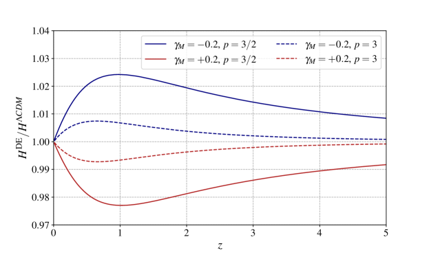
Figure 1: Hubble rate as a function of redshift in models with running Planck mass with $p=3/2$ (solid) and $p=3$ (dashed).

At the perturbative level, the CMB is sensitive to $\alpha_{\rm B}$ as well as $\alpha_{\rm M}$ mainly through the late-ISW effect. The impact on the ISW is given by Eq. (4.13), from which it follows that a positive $\alpha_{\rm M}$ slightly enhances the low-$\ell$ spectrum while a non-zero $\alpha_{\rm B}$ lowers the low-$\ell$’s until around $\alpha_{\rm B}\lesssim-0.1$, where its impact on the ISW becomes large and negative, leading to an overall increase. In addition, $\alpha_{\mathrm{M}}$ impacts the background by sourcing the dark energy density, see Sec. 3.1. A demonstration of this effect is displayed in Fig. 1, where we show the late-time Hubble rate as a function of redshift in two models with running Planck mass, relative to the $\Lambda$CDM one. For $p=3$ (dashed line) we see less than a percent difference for $\gamma_{\rm M}=\pm 0.2$, while for $p=3/2$ (solid line), in which the modifications to gravity are important at even earlier times, the difference exceeds 2%. Therefore, in addition to the late-ISW impact, $\alpha_{\rm M}$ also affects the location of the acoustic peaks through the angular diameter distance. This effect can be compensated for by a change of the Hubble rate today, and thus we expect a strong $\gamma_{\rm M}$–$H_{0}$ degeneracy.

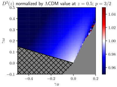
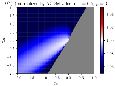
Figure 2: Growth factor $D^{2}$ at $z=0.5$ normalized to the $\Lambda$CDM value in the different models. The gray shaded regions indicate ghost instabilities, while the lighter gray hashed region show tachyonic instabilities. Upper left: Model I with $p=3/2$. Upper right: Model I with $p=3$. Lower: Model II with $p=3$.

In this work we include BAO measurements from both the SDSS and DESI surveys. BAO alone cannot constrain the braiding $\alpha_{\rm B}$, which only affects perturbations, but it can test background dynamics sourced by the running Planck mass (Model I) or a dark energy equation of state $w\neq-1$ (Model II).

Finally, the focus on this work is to test modified gravity with full-shape information from the BOSS redshift survey. In modified gravity, galaxy formation follows the modified Poisson equation (4.1). At the linear level, the growth factor $D(z)$ is altered by $\mu_{\Phi}(t)$. In Fig. 2, we display it as a function of the EFTofDE parameters in the different models at $z=0$. For non-zero braiding and running of the effective Planck mass (Model I), there is a clear degeneracy in the $\gamma_{\rm B}\simeq\gamma_{\rm M}$ direction, which was anticipated in the discussion below Eq. 4.8. Similarly, we see a degeneracy direction in the $\gamma_{\rm B}$–$w$ plane. Beyond the linear level, the $\mu_{\Phi,2}$- and $\mu_{\Phi,22}$-functions leave imprints on the power spectrum 1-loop correction. Lastly, galaxy clustering data is also sensitive to modification of the background via the Alcock-Paczynski effect.

For the galaxy power spectrum in real space, a modification of the growth factor at a specific redshift can be compensated for by a change of the initial amplitude of fluctuations as well as by the linear bias. On the other hand, redshift space distortions are impacted by the modified growth and furthermore observations at multiple redshift can aid in breaking degeneracies. All in all, we expect that BOSS power spectrum alone cannot sufficiently test a two-parameter extension within the EFTofDE, due to strong correlations with other cosmological parameters, in particular $A_{s}$ and $n_{s}$. This is in line with previous studies on modified gravity with the BOSS full-shape [81, 88]. Therefore it is useful to combine the BOSS full-shape with probes that well constrain $A_{s}$ and $n_{s}$, such as CMB measurements, as we will do below.

5 Results

In this section we list the datasets we use and perform the statistical inference on the EFTofDE models using cosmological data.

5.1 Datasets

In our analysis we combine a number of early and late time probes:

• Our CMB dataset comprises Planck TT,TE,EE high-$\ell$ data as well as low-$\ell$ TT and EE data [38]. We use the official PR3 likelihood for the statistical analysis [89]. This dataset is referred to as P18.

• We include the analysis of the full-shape power spectrum of luminous red galaxies (LRG) from the twelfth data release of the BOSS survey [36]. We analyze the monopole and quadrupole of the redshift-space power spectrum for both North and South Galactic Caps for each redshift bin, $z=0.32,0.57$. Following [81], we include modes up to $k_{\rm max}=0.20\,h$/Mpc for the lower redshift bin and $k_{\rm max}=0.23\,h$/Mpc for the higher one. This dataset is referred to as FS.

• To compare the constraining power of the full-shape power spectrum with BAO measurements in the BOSS dataset, we use the BOSS DR7 MGS (Main Galaxy Sample) [90] of galaxies in $z\in[0.07,0.2]$ as well as the BOSS DR12 [91] samples of galaxies in $z\in[0.2,0.5]$ and $z\in[0.4,0.6]$. We will refer to this dataset as BOSS BAO. We combine these with the recently released DESI DR1 BAO data, after excluding the two redshift bins that overlap with the BOSS ones. They consist of the LRG2 sample in $0.6<z<0.8$, the combined LRG3+ELG1 sample in $0.8<z<1.1$, the ELG2 sample in $1.1<z<1.6$, the quasar sample in $0.8<z<2.1$ and the Lyman-$\alpha$ Forest sample in $1.77<z<4.16$. We will refer to this dataset as DESI^∗.

When analyzing the data we always include the effects of neutrinos in the linear evolution, adopting the Planck prescription of one massive neutrino species with $m_{\nu}=0.06$ eV and two massless ones, with $N_{\rm eff}=2.0328$ [38]. The theory models are evaluated using a modified version of hi_class which accounts for our parameterization and modified background dynamics as described in Secs. 3.1 and 3.2.

For the full-shape power spectrum computation we use PyBird [48, 51], accordingly modified to include the linear and mildly non-linear effects of the EFTofDE model [53, 52]. The modifications are analogous to those of [81] and we refer the reader to this reference for details on the implementation. Specifically, following [48], we use the following set of nuisance parameters:

$$\{b_{1},c_{2},b_{3},c_{ct},c_{r,1},c_{\epsilon,0},c_{\epsilon,1},c_{\epsilon,2}\}\,,$$ (5.1)

where $b_{1}$ is the linear bias, $c_{2}$ is a combination of bias parameters appearing at second order, and $b_{3}$ is a bias parameter entering the third-order bias expansion. Additionally, $c_{ct}$ and $c_{r,1}$ are counterterms in redshift space, while $c_{\epsilon,0}$, $c_{\epsilon,1}$ and $c_{\epsilon,2}$ are stochastic terms. Since we are not sensitive to it, we set to zero the remaining combination of bias parameters appearing at second-order. We analytically marginalize on the third order bias $b_{3}$ and on all the counterterms and shot noise ones, following [51], using the same priors presented in [81].

We run MCMCs using the public code MontePython 3 [92, 93], varying the cosmological parameters

$$\{\omega_{b},\omega_{cdm},H_{0},A_{s},n_{s},\tau_{\mathrm{reio}}\}\,,$$ (5.2)

in combination with $\{\gamma_{\rm B},\gamma_{\rm M}\}$ for Model I and $\{\gamma_{\rm B},w\}$ for Model II, all with flat priors. We state convergence of the chains when the Gelman-Rubin $R-1$ value [94] is lower than $0.02$.

5.2 Parameter constraints

In this section, we present the results of the statistical inference on the EFTofDE. We will address the two models defined in Sec. 3.2. As for the time dependence, for Model II we analyze only the case $p=3$, as $p=3/2$ leads to tachyonic instabilities across the entire parameter space, except the $\Lambda$CDM limit.

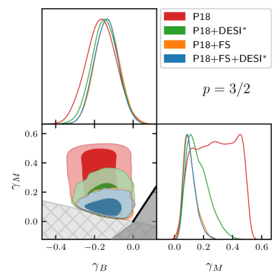
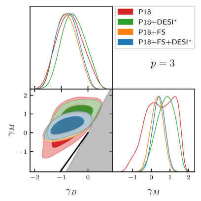
Figure 3: Posterior probabilities for Model I ($\gamma_{\rm B}$ and $\gamma_{\rm M}$ non-zero) with $p=3/2$ (left) and $p=3$ (right). The different dataset combination are defined in Sec. 5.1; note that DESI^∗ refers to a subset of the DESI BAO measurements in which the lowest redshift bins are removed, see that section for details. Regions of parameter space which lead to ghost or tachyonic instabilities are indicated by darker gray and lighter gray hashed shading, respectively. The region of parameter space which corresponds to Brans-Dicke gravity is indicated by the black line.

Figure 3 shows marginalized posterior distributions on the EFTofDE parameters in Model I, with $p=3/2$ (left panel) and $p=3$ (right panel). We find no significant evidence for modified gravity in any of the parameterizations. Additionally, there are no strong correlations between the EFTofDE parameters and the standard cosmological parameters, except for between $\alpha_{\rm M}$ and $H_{0}$ (the full triangle plot, including the standard cosmological parameters, is included in Appendix B). Using Planck alone, these parameters are almost perfectly degenerate because $\gamma_{\rm M}>0$ leads to a larger $H(z)$ at late times and vice versa. Adding late-time information on $H(z)$ from full-shape BOSS and/or DESI BAO data breaks this degeneracy, thus tightening constrains on $\gamma_{\rm M}$. For $p=3/2$, $\gamma_{\rm M}<0$ leads to tachyonic instabilities when $\gamma_{\rm B}<0$ and ghost instabilities when $\gamma_{\rm B}>0$, excluding these regions from our analysis. We find that $\gamma_{\rm M}<0.508$ at 2$\sigma$ for $p=3/2$ with Planck alone, improved to $\gamma_{\rm M}<0.203$ after adding the full-shape power spectrum, showing that adding LSS data shrinks the errorbars on this parameter by a factor of 2. Similarly, for $p=3$ we can constrain $\gamma_{\rm M}<1.83$ at 2$\sigma$ with Planck alone, updated to $\gamma_{\rm M}<0.964$ after adding the full-shape. We report the measured mean and 1$\sigma$ uncertainty from the statistical inference on the EFTofDE parameters and the Hubble constant in Table 1.

Next, we examine constraints on the braiding coefficient $\gamma_{\rm B}$. In all models there is a slight preference for a non-zero $\gamma_{\rm B}$ (e.g. for Planck+FS+DESI^∗ we obtain $\gamma_{\rm B}<-0.015$ and $\gamma_{\rm B}<-0.026$ at 2$\sigma$ for $p=3/2$ and $p=3$, respectively), primarily driven by low-$\ell$ CMB data. This preference has also been reported by other studies using CMB data, e.g. [28, 73, 34]. For $p=3$ the $\gamma_{\rm B}$–$\gamma_{\rm M}$ degeneracy-direction for the Planck-alone analysis is evident, as shown at the level of the growth factor in Fig. 2. The degeneracy is broken by late-time background impact of $\gamma_{\rm M}$ with full-shape (orange) or full-shape and DESI (blue) in the right panel of Fig. 3. For $p=3/2$, the degeneracy is less visible due to the longer integrated background effect of $\gamma_{\rm M}$. We find that adding full-shape information somewhat improves the $2\sigma$ bound on the braiding coefficient over Planck alone, from $\gamma_{\rm B}>-0.33$ to $\gamma_{\rm B}>-0.26$ in the $p=3/2$ case and from $\gamma_{\rm B}>-1.62$ to $\gamma_{\rm B}>-1.53$ in the $p=3$ case.

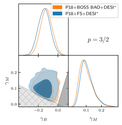
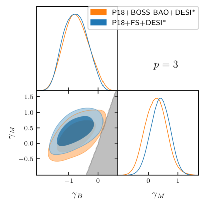
Figure 4: Same as Fig. 3. We compare the posterior probabilities when exchanging BOSS full-shape information with BOSS BAO data.

In Fig. 4 we compare the constraining power of using the full-shape power spectrum versus BAO measurements (see Sec. 5.1 for a description of the BAO measurements included) of BOSS in the modified gravity model with non-zero braiding and evolving Planck mass. We perform the comparison including Planck and DESI observations, and find no significant improvement of using the full-shape versus BAO only within these dataset combinations. This result emphasizes that Planck CMB measurements best constrain the braiding coefficient, while the background impact dominate the constraints on the evolution of the Planck mass.

Next, we discuss the results of the statistical inference of Model II, which considers a non-zero braiding on top of a $w$CDM background. As mentioned above, we take $p=3$ only, as $p=3/2$ leads to tachyonic instabilities for $\gamma_{\rm B}\neq 0$. The posterior probabilities on $\gamma_{\rm B}$ and $w$ are shown in the left panel of Fig. 5. We observe no significant evidence for braiding effects; utilizing Planck, full-shape and DESI BAO data we obtain a lower 2$\sigma$ bound $\gamma_{\rm B}>-1.46$. As for Model I, the BOSS full-shape power spectrum information does not add significant additional information that can further constrain $\gamma_{\rm B}$ over Planck CMB data.

As is well known, Planck alone allows for a wide range of the dark energy equation of state $w$ [38]. The red contour in Fig. 5 reproduces this conclusion, and the full posterior in App. B shows a strong degeneracy between $w$ and $H_{0}$ due to the insensitivity of CMB alone on late-time modifications. Adding late-time information from DESI BAO aids in breaking the degeneracy, allowing us to measure $w=-1.12\pm 0.17$ at 2$\sigma$. With the full-shape power spectrum, we can tighten the constraint on the equation of state parameter to $w=-1.07\pm 0.10$ at 2$\sigma$ using Planck + FS + DESI^∗ (blue contour), showing a $40\%$ improvement. The joint posterior probability for $\gamma_{\rm B}$ and $w$ in analyses including full-shape information (orange and blue) displays the same degeneracy direction as shown for the growth factor in Fig. 2. This degeneracy direction is constrained by Planck’s sensitivity to braiding at $\gamma_{\rm B}=-0.80^{+0.41}_{-0.32}$.

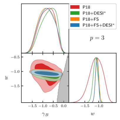
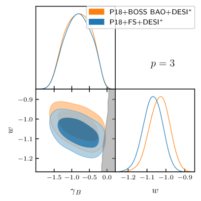
Figure 5: Posterior probabilities for Model II ($\gamma_{\rm B}$ and $\gamma_{\rm M}$ non-zero) for $p=3$. See Sec. 5.1 for definitions of dataset combinations. Ghost instabilities are indicated by the shaded area. Left: Comparison of statistical inference with BOSS full-shape information and BOSS BAO measurements.

Lastly, we compare the full-shape constraints of Model II with an analysis using SDSS BAO measurements. Specifically, we compare Planck + FS + DESI^∗ to Planck + SDSS BAO + DESI^∗. The result is shown in the right panel of Fig. 5. As with Model I, we see similar constraining power in both cases, with a slight shift of the posterior for $w$. Thus, we conclude that within this combination of experiments, Planck is most sensitive to the braiding parameter, while the background impact of $w$ dominates such that BOSS full-shape information is not significantly more sensitive to it than BAO alone.

In summary, we find in both models that Planck CMB measurements are mostly sensitive to the braiding parameter $\gamma_{\rm B}$. On the other hand, the $w$ and $\alpha_{\rm M}$ parameters are poorly constrained by CMB alone, mainly because of the degeneracy with $H_{0}$, see Figs. 7 – 9. LSS improves the bounds on these two parameters. Present DESI data do not add much information over that extracted by BOSS data. The comparison between FS and BAO gives similar results, meaning that the main role of LSS is to remove the $\alpha_{\rm M}$-$H_{0}$ or $w$-$H_{0}$ degeneracies via the late-time geometrical information encoded in the BAO’s. Nonlinearities, in particular the extra dependence on $\alpha_{\rm M}$ of the non-linear effects shown in Eq. (4.8) seem to play a marginal role. However, this will likely change once new FS data from DESI and Euclid, will be available.

Table 1: Measured mean values and 1-$\sigma$ uncertainty on the EFTofDE parameters as well as the Hubble constant.

		P18	P18 + DESI∗	P18 + FS	P18 + FS + DESI∗
Model I	$\gamma_{\rm B}$	$-0.166_{-0.083}^{+0.082}$	$-0.146_{-0.07}^{+0.068}$	$-0.135_{-0.065}^{+0.062}$	$-0.140_{-0.062}^{+0.062}$
$p=3/2$	$\gamma_{\rm M}$	$0.29_{-0.12}^{+0.18}$	$0.163_{-0.097}^{+0.052}$	$0.106_{-0.054}^{+0.029}$	$0.106_{-0.05}^{+0.028}$
	$H_{0}$	$73.12_{-2.2}^{+3.1}$	$70.82_{-1.5}^{+1.0}$	$69.77_{-0.86}^{+0.76}$	$69.82_{-0.8}^{+0.65}$
Model I	$\gamma_{\rm B}$	$-0.68_{-0.56}^{+0.48}$	$-0.54_{-0.48}^{+0.44}$	$-0.80_{-0.44}^{+0.39}$	$-0.77_{-0.47}^{+0.37}$
$p=3$	$\gamma_{\rm M}$	$0.47_{-0.71}^{+0.94}$	$0.77_{-0.48}^{+0.55}$	$0.31_{-0.34}^{+0.34}$	$0.41_{-0.31}^{+0.35}$
	$H_{0}$	$69.85_{-2.6}^{+4.4}$	$71.16_{-1.5}^{+2.3}$	$69.39_{-1.3}^{+1.4}$	$69.87_{-1.1}^{+1.2}$
Model II	$\gamma_{\rm B}$	$-0.80_{-0.32}^{+0.41}$	$-0.73_{-0.27}^{+0.47}$	$-0.82_{-0.40}^{+0.40}$	$-0.82_{-0.38}^{+0.42}$
$p=3$	$w$	$-1.10_{-0.22}^{+0.27}$	$-1.116_{-0.083}^{+0.088}$	$-1.055_{-0.057}^{+0.058}$	$-1.069_{-0.05}^{+0.054}$
	$H_{0}$	$71.49_{-9.7}^{+6.9}$	$71.71_{-2.8}^{+2.4}$	$69.7_{-1.6}^{+1.6}$	$70.2_{-1.5}^{+1.3}$

The 1$\sigma$ measurements on the EFTofDE parameters are given in Table 1, while the full list of all cosmological parameters is given in Table 2.

6 Conclusion

We have performed a combined analysis of CMB and LSS data, including the recent BAO measurement from the DESI collaboration, constraining modified gravity and dark energy properties using the EFTofDE framework. The main new features of our pipeline are a consistent treatment of the linear background equations, as discussed in Sec. 3.1, and a consistent treatment of dark matter nonlinearities, see Sec. 4.1.

We have shown that the combination with LSS data can improve the constraints on the EFTofDE parameter space compared to CMB alone analyses. This is true for the modified gravity parameter $\gamma_{\rm M}$, which quantifies the running of the Planck mass, and the equation of state of dark energy $w$. The main information provided by current LSS observations is contained in BAO’s, which allow to break the geometrical degeneracy between the Hubble rate and parameters that affect the background evolution, either the dark energy equation of state or the running of the Planck mass. One goal of this work was to assess at which level the remaining information encoded in the power spectrum shape is accessible, in particular from nonlinear scales. For the BOSS data and covariances we do not detect a significant improvement in the constraints on the EFTofDE parameters. This becomes clear when looking to the constraints on the braiding parameter $\gamma_{\rm B}$, which affects the perturbations without altering the background evolution: this parameter is mostly constrained by CMB. Adding LSS information, either BAO alone or full-shape power spectrum, has a negligible impact. However, future full shape data from Euclid and DESI will likely change the situation, given their large observed volumes and number densities, thus requiring consistent nonlinear pipelines for their analyses based on the EFTofLSS, as the one developed in this work. Moreover, the wide range of redshifts that will be observed will definitely improve our understanding of background evolution, shedding light on dark energy dynamics.

Including higher-order correlation functions such as the bispectrum is not expected to significantly ameliorate the current situation, given its low signal-to-noise ratio. It has been shown that the main contribution from the bispectrum is an improved estimate for the non-linear bias parameters and a $\sim 5-15\%$ improvement on cosmological parameters assuming $\Lambda$CDM [95, 96, 97]. Even for beyond-$\Lambda$CDM models, such as including new dark matter species or non-standard dark energy dynamics, adding the LSS bispectrum does not significantly improve the constraints [98, 99].

Moreover, in the EFTofDE, parameters appear at the level of the action, that is, of the equations of motion. In order to solve the equations of motion and derive the observables, a time-dependence of these functions needs to be assumed. In this paper we tested two different power laws, see Eq. (3.13). The corresponding constraints are shown for instance in Fig. 3, which shows that these two choices correspond to two very different models. Therefore, the question arises of how to treat the model dependence hidden in the time-dependence. A possible, agnostic, alternative would be to parameterize directly the observables, in place of the equations of motion, exploiting symmetries, as in the bootstrap approach of Refs. [100, 101]. This would require introducing new coefficients parameterizing the ISW and lensing effects and a set of new parameters for any redshift bin of LSS data. The design of strategies to optimize the trade-off between model-independence and parameter proliferation is therefore a crucial issue in the exploration of physics beyond $\Lambda$CDM. Most of the information loss in LSS arises due to the ignorance about the non-linear mapping from dark matter to galaxies parameterized by the galaxy biases. One possible way to tackle this is putting physically motivated priors on them, using e.g. analytical recipes [102, 103, 104, 105, 106, 107, 108], or numerical simulations [109].

We leave all these possible extensions of our work to future studies.

Acknowledgments: We are grateful to Emilio Bellini, Guido D’Amico, Lorenzo Piga and Anton Chudaykin for useful discussions related to this work. MM and MP acknowledge support by the MIUR Progetti di Ricerca di Rilevante Interesse Nazionale (PRIN) Bando 2022 - grant 20228RMX4A. PT and FV acknowledge support by the ANR Project COLSS (ANR-21-CE31-0029). This work was granted access to the CCRT High-Performance Computing (HPC) facility under the Grant CCRT2024-taulepet awarded by the Fundamental Research Division (DRF) of CEA. The package GetDist [110] was used to create the plots and compute the summary statistics.

Appendix A Tensor speed excess

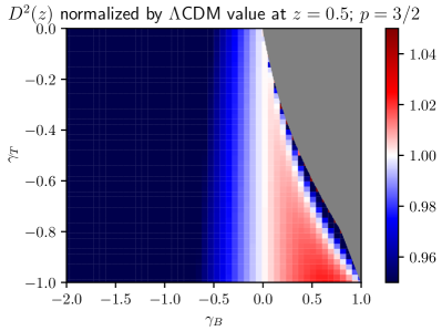
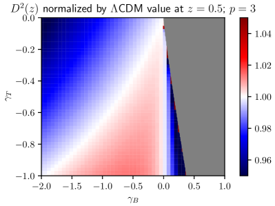
Figure 6: Growth factor $D^{2}$ at $z=0.5$ normalized to the $\Lambda$CDM value in models with non-zero braiding and tensor speed excess ($\Lambda$CDM background). The gray shaded regions indicate ghost instabilities. Left: $p=3/2$ and right: $p=3$.

In this appendix we consider the impact of tensor speed excess $\alpha_{\rm T}$ on LSS. We set $\alpha_{\rm M}=0$ and $w=-1$ for simplicity and choose $\alpha_{\rm T}=\gamma_{\rm T}(a/a_{0})^{p}$. Then the function $\nu$ (see Eq. (2.9)) is given by

$$\nu=-(1+\alpha_{\rm B})\left[\alpha_{\rm B}+\alpha_{\rm T}(1+\alpha_{\rm B})\right]+\left(\frac{3}{2}\Omega_{\rm m}-p\right)\alpha_{\rm B}\,,$$ (A.1)

and moreover we obtain

$$\mu_{\Phi}=1+\alpha_{\rm T}+\frac{\left[\alpha_{\rm T}+\alpha_{\rm B}(1+\alpha_{\rm T})\right]^{2}}{\nu}\,.$$ (A.2)

When $p=3/2$, the last parenthesis of Eq. (A.1) is close to zero until very late times, resulting in a cancellation of $\alpha_{\rm T}$ at leading order in $\mu_{\Phi}$. Thus, at leading order the Poisson equation is unaltered by the tensor speed excess, as can be seen in the left panel of Fig. 6, which displays the growth factor $D^{2}(z)$ at $z=0.5$ in this model. For $p=3$, we can instead identify a degeneracy direction in which $\mu_{\Phi}=1$:

$$\alpha_{\rm T}=-\frac{2\alpha_{\rm B}}{-4+2\alpha_{\rm B}+3\Omega_{\rm m}}\,.$$ (A.3)

This leads to a region of parameter space which is unaffected by the modified gravity parameters, as exemplified by the right panel of Fig. 6. (Note that due to the growth factor being an integrated quantity of $\mu_{\Phi}$ and the $\alpha$s and $\Omega_{\rm m}$ having different time-dependencies, the degeneracy in $D$ does not simply have the functional form of Eq. (A.3).)

In conclusion, for the parameterizations considered here, the tensor speed excess impact on the Poisson equation is too small for LSS data to be sensitive to it.

Appendix B Full parameter constraints

We display triangle plots of the standard cosmological parameters and the EFTofDE parameters in Fig. 7 (Model I with $p=3/2$), Fig. 8 (Model I with $p=3$) and Fig. 9 (Model II with $p=3$). The measured mean and 1$\sigma$ on the parameters are reported in Table 2.

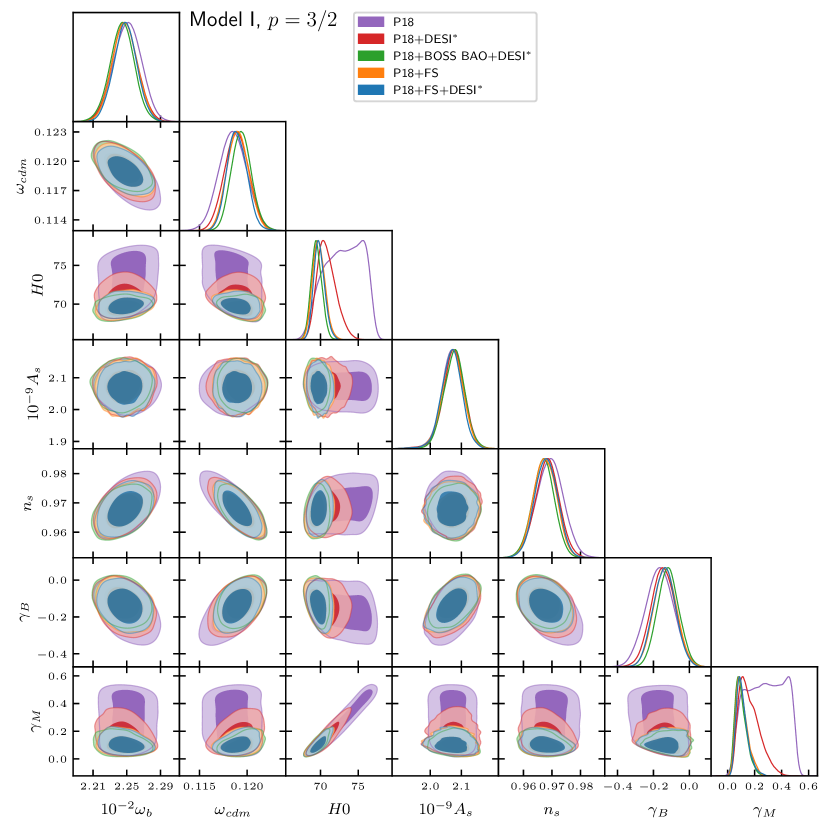
Figure 7: Full posterior probability triangle plot for Model I with $p=3/2$.

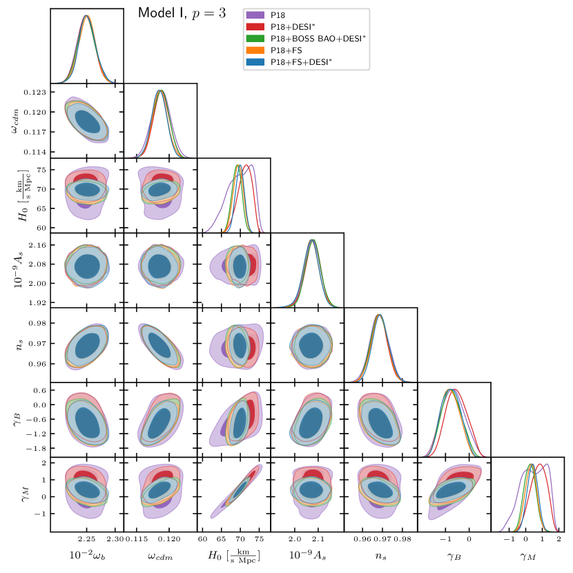
Figure 8: Full posterior probability triangle plot for Model I with $p=3$.

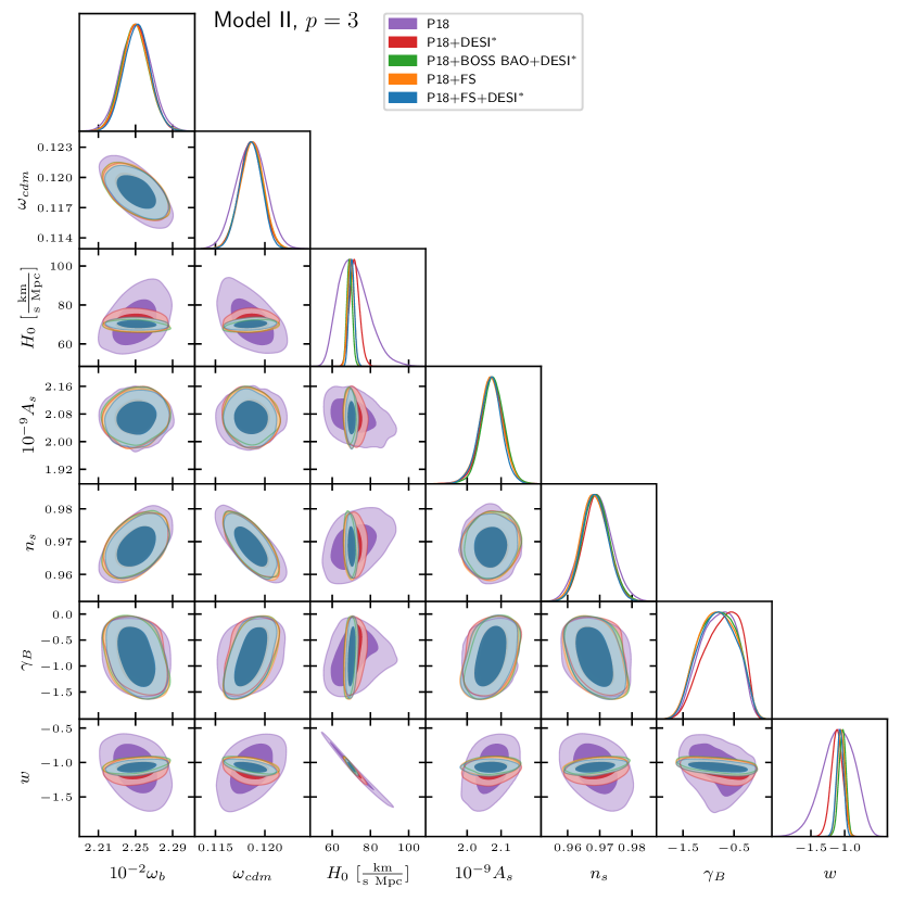
Figure 9: Full posterior probability triangle plot for Model II with $p=3$.

Table 2: The inferred mean and 1$\sigma$ uncertainty on all cosmological parameters. We quote also the maximum likelihood.

		P18	P18 + DESI∗	P18 + FS	P18 + FS + DESI∗
Model I	$100\omega_{b}$	$2.251_{-0.017}^{+0.018}$	$2.247_{-0.016}^{+0.015}$	$2.248_{-0.015}^{+0.014}$	$2.248_{-0.013}^{+0.014}$
$p=3/2$	$\omega_{cdm}$	$0.1185_{-0.0016}^{+0.0016}$	$0.1189_{-0.0013}^{+0.0013}$	$0.119_{-0.0012}^{+0.0011}$	$0.1189_{-0.0011}^{+0.001}$
	$H_{0}$	$73.12_{-2.2}^{+3.1}$	$70.82_{-1.5}^{+1}$	$69.77_{-0.86}^{+0.76}$	$69.82_{-0.8}^{+0.65}$
	$10^{+9}A_{s}$	$2.072_{-0.038}^{+0.039}$	$2.075_{-0.011}^{+0.13}$	$2.071_{-0.062}^{+0.049}$	$2.068_{-0.08}^{+0.069}$
	$n_{s}$	$0.9693_{-0.0051}^{+0.005}$	$0.9684_{-0.0042}^{+0.0044}$	$0.9676_{-0.0042}^{+0.0042}$	$0.968_{-0.0042}^{+0.004}$
	$\tau_{\mathrm{reio}}$	$0.0498_{-0.0086}^{+0.0093}$	$0.04983_{-0.0077}^{+0.0089}$	$0.04875_{-0.0078}^{+0.0084}$	$0.04827_{-0.0073}^{+0.0085}$
	$\gamma_{\rm B}$	$-0.1655_{-0.083}^{+0.082}$	$-0.1464_{-0.07}^{+0.068}$	$-0.1351_{-0.065}^{+0.062}$	$-0.1399_{-0.062}^{+0.062}$
	$\gamma_{\rm M}$	$0.2865_{-0.12}^{+0.18}$	$0.1629_{-0.097}^{+0.052}$	$0.1061_{-0.054}^{+0.029}$	$0.1061_{-0.05}^{+0.028}$
	$-\ln{\cal L}_{\mathrm{min}}$	$1388.58$	$1391.69$	$1460.97$	$1464.45$
Model I	$100\omega_{b}$	$2.249_{-0.02}^{+0.017}$	$2.249_{-0.015}^{+0.015}$	$2.251_{-0.014}^{+0.015}$	$2.251_{-0.016}^{+0.014}$
$p=3$	$\omega_{cdm}$	$0.1187_{-0.0016}^{+0.0016}$	$0.1188_{-0.0012}^{+0.0013}$	$0.1186_{-0.0012}^{+0.0012}$	$0.1185_{-0.0012}^{+0.0011}$
	$H_{0}$	$69.85_{-2.6}^{+4.4}$	$71.16_{-1.5}^{+2.3}$	$69.39_{-1.3}^{+1.4}$	$69.87_{-1.1}^{+1.2}$
	$10^{+9}A_{s}$	$2.075_{-0.039}^{+0.14}$	$2.077_{-0.075}^{+0.039}$	$2.07_{-0.076}^{+0.039}$	$2.069_{-0.033}^{+0.034}$
	$n_{s}$	$0.9684_{-0.0052}^{+0.0053}$	$0.9683_{-0.004}^{+0.0042}$	$0.9685_{-0.0041}^{+0.0043}$	$0.969_{-0.0044}^{+0.0039}$
	$\tau_{\mathrm{reio}}$	$0.05016_{-0.0089}^{+0.0094}$	$0.05062_{-0.0073}^{+0.0083}$	$0.04934_{-0.0075}^{+0.0081}$	$0.04913_{-0.0074}^{+0.0084}$
	$\gamma_{\rm B}$	$-0.6751_{-0.56}^{+0.48}$	$-0.5371_{-0.48}^{+0.44}$	$-0.8006_{-0.44}^{+0.39}$	$-0.7725_{-0.47}^{+0.37}$
	$\gamma_{\rm M}$	$0.4727_{-0.71}^{+0.94}$	$0.7675_{-0.48}^{+0.55}$	$0.3096_{-0.34}^{+0.34}$	$0.4096_{-0.31}^{+0.35}$
	$-\ln{\cal L}_{\mathrm{min}}$	$1388.28$	$1390.91$	$1460.87$	$1463.92$
Model II	$100\omega_{b}$	$2.251_{-0.017}^{+0.015}$	$2.251_{-0.015}^{+0.014}$	$2.25_{-0.014}^{+0.015}$	$2.252_{-0.015}^{+0.014}$
$p=3$	$\omega_{cdm}$	$0.1186_{-0.0015}^{+0.0016}$	$0.1186_{-0.0011}^{+0.0012}$	$0.1187_{-0.0011}^{+0.0012}$	$0.1186_{-0.0011}^{+0.0012}$
	$H_{0}$	$71.49_{-9.7}^{+6.9}$	$71.71_{-2.8}^{+2.4}$	$69.7_{-1.6}^{+1.6}$	$70.2_{-1.5}^{+1.3}$
	$10^{+9}A_{s}$	$2.071_{-0.078}^{+0.041}$	$2.072_{-0.033}^{+0.035}$	$2.069_{-0.033}^{+0.035}$	$2.067_{-0.033}^{+0.033}$
	$n_{s}$	$0.9689_{-0.0048}^{+0.0048}$	$0.969_{-0.0041}^{+0.0042}$	$0.9683_{-0.0043}^{+0.0042}$	$0.9685_{-0.0042}^{+0.0039}$
	$\tau_{\mathrm{reio}}$	$0.04946_{-0.0076}^{+0.0086}$	$0.04986_{-0.0079}^{+0.0084}$	$0.04901_{-0.0076}^{+0.0083}$	$0.04886_{-0.0073}^{+0.0081}$
	$\gamma_{\rm B}$	$-0.7992_{-0.32}^{+0.41}$	$-0.7273_{-0.27}^{+0.47}$	$-0.8228_{-0.4}^{+0.4}$	$-0.8176_{-0.38}^{+0.42}$
	$w$	$-1.098_{-0.22}^{+0.27}$	$-1.116_{-0.083}^{+0.088}$	$-1.055_{-0.057}^{+0.058}$	$-1.069_{-0.05}^{+0.054}$
	$-\ln{\cal L}_{\mathrm{min}}$	$1387.84$	$1390.3$	$1460.62$	$1463.72$

References

- [1] eBOSS Collaboration, S. Alam et. al., “Completed SDSS-IV extended Baryon Oscillation Spectroscopic Survey: Cosmological implications from two decades of spectroscopic surveys at the Apache Point Observatory,” Phys. Rev. D 103 (2021), no. 8 083533, 2007.08991.
- [2] DESI Collaboration, A. Aghamousa et. al., “The DESI Experiment Part I: Science,Targeting, and Survey Design,” 1611.00036.
- [3] Euclid Collaboration, Y. Mellier et. al., “Euclid. I. Overview of the Euclid mission,” 2405.13491.
- [4] A. Cimatti, R. Laureijs, B. Leibundgut, S. Lilly, R. Nichol, A. Refregier, P. Rosati, M. Steinmetz, N. Thatte, and E. Valentijn, “Euclid Assessment Study Report for the ESA Cosmic Visions,” 0912.0914.
- [5] Euclid Collaboration, A. Blanchard et. al., “Euclid preparation. VII. Forecast validation for Euclid cosmological probes,” Astron. Astrophys. 642 (2020) A191, 1910.09273.
- [6] L. Amendola et. al., “Cosmology and fundamental physics with the Euclid satellite,” Living Rev. Rel. 21 (2018), no. 1 2, 1606.00180.
- [7] P. Creminelli, G. D’Amico, J. Norena, and F. Vernizzi, “The Effective Theory of Quintessence: the w-1 Side Unveiled,” JCAP 02 (2009) 018, 0811.0827.
- [8] T. Baker, P. G. Ferreira, C. Skordis, and J. Zuntz, “Towards a fully consistent parameterization of modified gravity,” Phys. Rev. D 84 (2011) 124018, 1107.0491.
- [9] R. A. Battye and J. A. Pearson, “Effective action approach to cosmological perturbations in dark energy and modified gravity,” JCAP 07 (2012) 019, 1203.0398.
- [10] G. Gubitosi, F. Piazza, and F. Vernizzi, “The Effective Field Theory of Dark Energy,” JCAP 1302 (2013) 032, 1210.0201. [JCAP1302,032(2013)].
- [11] T. Baker, P. G. Ferreira, and C. Skordis, “The Parameterized Post-Friedmann framework for theories of modified gravity: concepts, formalism and examples,” Phys. Rev. D 87 (2013), no. 2 024015, 1209.2117.
- [12] J. K. Bloomfield, E. E. Flanagan, M. Park, and S. Watson, “Dark energy or modified gravity? An effective field theory approach,” JCAP 08 (2013) 010, 1211.7054.
- [13] J. Gleyzes, D. Langlois, F. Piazza, and F. Vernizzi, “Essential Building Blocks of Dark Energy,” JCAP 08 (2013) 025, 1304.4840.
- [14] J. Bloomfield, “A Simplified Approach to General Scalar-Tensor Theories,” JCAP 12 (2013) 044, 1304.6712.
- [15] R. A. Battye and J. A. Pearson, “Computing model independent perturbations in dark energy and modified gravity,” JCAP 03 (2014) 051, 1311.6737.
- [16] J. Gleyzes, D. Langlois, and F. Vernizzi, “A unifying description of dark energy,” Int. J. Mod. Phys. D23 (2014) 1443010, 1411.3712.
- [17] C. Skordis, A. Pourtsidou, and E. J. Copeland, “Parametrized post-Friedmannian framework for interacting dark energy theories,” Phys. Rev. D 91 (2015), no. 8 083537, 1502.07297.
- [18] M. Lagos, T. Baker, P. G. Ferreira, and J. Noller, “A general theory of linear cosmological perturbations: scalar-tensor and vector-tensor theories,” JCAP 08 (2016) 007, 1604.01396.
- [19] I. Zlatev, L.-M. Wang, and P. J. Steinhardt, “Quintessence, cosmic coincidence, and the cosmological constant,” Phys. Rev. Lett. 82 (1999) 896–899, astro-ph/9807002.
- [20] G. R. Dvali, G. Gabadadze, and M. Porrati, “4-D gravity on a brane in 5-D Minkowski space,” Phys. Lett. B 485 (2000) 208–214, hep-th/0005016.
- [21] C. Armendariz-Picon, V. F. Mukhanov, and P. J. Steinhardt, “A Dynamical solution to the problem of a small cosmological constant and late time cosmic acceleration,” Phys. Rev. Lett. 85 (2000) 4438–4441, astro-ph/0004134.
- [22] S. M. Carroll, A. De Felice, V. Duvvuri, D. A. Easson, M. Trodden, and M. S. Turner, “The Cosmology of generalized modified gravity models,” Phys. Rev. D 71 (2005) 063513, astro-ph/0410031.
- [23] G. W. Horndeski, “Second-order scalar-tensor field equations in a four-dimensional space,” Int. J. Theor. Phys. 10 (1974) 363–384.
- [24] C. Deffayet, X. Gao, D. A. Steer, and G. Zahariade, “From k-essence to generalised Galileons,” Phys. Rev. D 84 (2011) 064039, 1103.3260.
- [25] M. Raveri, B. Hu, N. Frusciante, and A. Silvestri, “Effective Field Theory of Cosmic Acceleration: constraining dark energy with CMB data,” Phys. Rev. D 90 (2014), no. 4 043513, 1405.1022.
- [26] J. Gleyzes, D. Langlois, M. Mancarella, and F. Vernizzi, “Effective Theory of Dark Energy at Redshift Survey Scales,” JCAP 02 (2016) 056, 1509.02191.
- [27] E. Bellini, A. J. Cuesta, R. Jimenez, and L. Verde, “Constraints on deviations from CDM within Horndeski gravity,” JCAP 02 (2016) 053, 1509.07816. [Erratum: JCAP 06, E01 (2016)].
- [28] J. Noller and A. Nicola, “Cosmological parameter constraints for Horndeski scalar-tensor gravity,” Phys. Rev. D 99 (2019), no. 10 103502, 1811.12928.
- [29] A. Spurio Mancini, R. Reischke, V. Pettorino, B. M. Schäfer, and M. Zumalacárregui, “Testing (modified) gravity with 3D and tomographic cosmic shear,” Mon. Not. Roy. Astron. Soc. 480 (2018), no. 3 3725–3738, 1801.04251.
- [30] A. Spurio Mancini, F. Köhlinger, B. Joachimi, V. Pettorino, B. M. Schäfer, R. Reischke, E. van Uitert, S. Brieden, M. Archidiacono, and J. Lesgourgues, “KiDS + GAMA: constraints on horndeski gravity from combined large-scale structure probes,” Mon. Not. Roy. Astron. Soc. 490 (2019), no. 2 2155–2177, 1901.03686.
- [31] L. Perenon, J. Bel, R. Maartens, and A. de la Cruz-Dombriz, “Optimising growth of structure constraints on modified gravity,” JCAP 06 (2019) 020, 1901.11063.
- [32] J. Noller, “Cosmological constraints on dark energy in light of gravitational wave bounds,” Phys. Rev. D 101 (2020), no. 6 063524, 2001.05469.
- [33] G. Brando, F. T. Falciano, E. V. Linder, and H. E. S. Velten, “Modified gravity away from a CDM background,” JCAP 11 (2019) 018, 1904.12903.
- [34] A. Chudaykin and M. Kunz, “Modified gravity interpretation of the evolving dark energy in light of DESI data,” 2407.02558.
- [35] N. Frusciante and L. Perenon, “Effective field theory of dark energy: A review,” Phys. Rept. 857 (2020) 1–63, 1907.03150.
- [36] BOSS Collaboration, H. Gil-Marín et. al., “The clustering of galaxies in the SDSS-III Baryon Oscillation Spectroscopic Survey: RSD measurement from the LOS-dependent power spectrum of DR12 BOSS galaxies,” Mon. Not. Roy. Astron. Soc. 460 (2016), no. 4 4188–4209, 1509.06386.
- [37] DESI Collaboration, A. G. Adame et. al., “DESI 2024 VI: Cosmological Constraints from the Measurements of Baryon Acoustic Oscillations,” 2404.03002.
- [38] Planck Collaboration, N. Aghanim et. al., “Planck 2018 results. VI. Cosmological parameters,” Astron. Astrophys. 641 (2020) A6, 1807.06209. [Erratum: Astron.Astrophys. 652, C4 (2021)].
- [39] M. Zumalacárregui, E. Bellini, I. Sawicki, J. Lesgourgues, and P. G. Ferreira, “hi_class: Horndeski in the Cosmic Linear Anisotropy Solving System,” JCAP 08 (2017) 019, 1605.06102.
- [40] E. Bellini, I. Sawicki, and M. Zumalacárregui, “hi_class: Background Evolution, Initial Conditions and Approximation Schemes,” JCAP 02 (2020) 008, 1909.01828.
- [41] D. Baumann, A. Nicolis, L. Senatore, and M. Zaldarriaga, “Cosmological Non-Linearities as an Effective Fluid,” JCAP 07 (2012) 051, 1004.2488.
- [42] J. J. M. Carrasco, M. P. Hertzberg, and L. Senatore, “The Effective Field Theory of Cosmological Large Scale Structures,” JHEP 09 (2012) 082, 1206.2926.
- [43] L. Senatore, “Bias in the Effective Field Theory of Large Scale Structures,” JCAP 11 (2015) 007, 1406.7843.
- [44] A. Perko, L. Senatore, E. Jennings, and R. H. Wechsler, “Biased Tracers in Redshift Space in the EFT of Large-Scale Structure,” 1610.09321.
- [45] M. M. Ivanov, Effective Field Theory for Large-Scale Structure. 2023. 2212.08488.
- [46] G. Cabass, M. M. Ivanov, M. Lewandowski, M. Mirbabayi, and M. Simonović, “Snowmass white paper: Effective field theories in cosmology,” Phys. Dark Univ. 40 (2023) 101193, 2203.08232.
- [47] M. M. Ivanov, M. Simonović, and M. Zaldarriaga, “Cosmological Parameters from the BOSS Galaxy Power Spectrum,” JCAP 05 (2020) 042, 1909.05277.
- [48] G. D’Amico, J. Gleyzes, N. Kokron, K. Markovic, L. Senatore, P. Zhang, F. Beutler, and H. Gil-Marín, “The Cosmological Analysis of the SDSS/BOSS data from the Effective Field Theory of Large-Scale Structure,” JCAP 05 (2020) 005, 1909.05271.
- [49] G. D’Amico, M. Lewandowski, L. Senatore, and P. Zhang, “Limits on primordial non-Gaussianities from BOSS galaxy-clustering data,” 2201.11518.
- [50] G. Cabass, M. M. Ivanov, O. H. E. Philcox, M. Simonović, and M. Zaldarriaga, “Constraints on Single-Field Inflation from the BOSS Galaxy Survey,” Phys. Rev. Lett. 129 (2022), no. 2 021301, 2201.07238.
- [51] G. D’Amico, L. Senatore, and P. Zhang, “Limits on CDM from the EFTofLSS with the PyBird code,” JCAP 01 (2021) 006, 2003.07956.
- [52] G. Cusin, M. Lewandowski, and F. Vernizzi, “Dark Energy and Modified Gravity in the Effective Field Theory of Large-Scale Structure,” JCAP 04 (2018) 005, 1712.02783.
- [53] G. Cusin, M. Lewandowski, and F. Vernizzi, “Nonlinear Effective Theory of Dark Energy,” JCAP 04 (2018) 061, 1712.02782.
- [54] B. Bose, K. Koyama, M. Lewandowski, F. Vernizzi, and H. A. Winther, “Towards Precision Constraints on Gravity with the Effective Field Theory of Large-Scale Structure,” JCAP 04 (2018) 063, 1802.01566.
- [55] Euclid Collaboration, N. Frusciante et. al., “Euclid: Constraining linearly scale-independent modifications of gravity with the spectroscopic and photometric primary probes,” 2306.12368.
- [56] Euclid Collaboration, S. Casas et. al., “Euclid: Constraints on f(R) cosmologies from the spectroscopic and photometric primary probes,” 2306.11053.
- [57] Euclid Collaboration, B. Bose et. al., “Euclid preparation. XLIV. Modelling spectroscopic clustering on mildly nonlinear scales in beyond-CDM models,” 2311.13529.
- [58] Euclid Collaboration, K. Koyama et. al., “Euclid preparation. Simulations and nonlinearities beyond CDM. 4. Constraints on models from the photometric primary probes,” 2409.03524.
- [59] E. Bellini and I. Sawicki, “Maximal freedom at minimum cost: linear large-scale structure in general modifications of gravity,” JCAP 1407 (2014) 050, 1404.3713.
- [60] J. Gleyzes, D. Langlois, F. Piazza, and F. Vernizzi, “Healthy theories beyond Horndeski,” Phys. Rev. Lett. 114 (2015), no. 21 211101, 1404.6495.
- [61] M. Zumalacárregui and J. García-Bellido, “Transforming gravity: from derivative couplings to matter to second-order scalar-tensor theories beyond the Horndeski Lagrangian,” Phys.Rev. D89 (2014), no. 6 064046, 1308.4685.
- [62] D. Langlois and K. Noui, “Degenerate higher derivative theories beyond Horndeski: evading the Ostrogradski instability,” JCAP 1602 (2016) 034, 1510.06930.
- [63] J. Gleyzes, D. Langlois, F. Piazza, and F. Vernizzi, “Exploring gravitational theories beyond Horndeski,” JCAP 02 (2015) 018, 1408.1952.
- [64] D. Langlois, M. Mancarella, K. Noui, and F. Vernizzi, “Effective Description of Higher-Order Scalar-Tensor Theories,” JCAP 1705 (2017) 033, 1703.03797.
- [65] C. Deffayet, O. Pujolas, I. Sawicki, and A. Vikman, “Imperfect Dark Energy from Kinetic Gravity Braiding,” JCAP 10 (2010) 026, 1008.0048.
- [66] C. Brans and R. H. Dicke, “Mach’s principle and a relativistic theory of gravitation,” Phys. Rev. 124 (1961) 925–935.
- [67] A. Nicolis, R. Rattazzi, and E. Trincherini, “The Galileon as a local modification of gravity,” Phys. Rev. D 79 (2009) 064036, 0811.2197.
- [68] LIGO Scientific, Virgo Collaboration, B. P. Abbott et. al., “GW170817: Observation of Gravitational Waves from a Binary Neutron Star Inspiral,” Phys. Rev. Lett. 119 (2017), no. 16 161101, 1710.05832.
- [69] P. Creminelli and F. Vernizzi, “Dark Energy after GW170817 and GRB170817A,” Phys. Rev. Lett. 119 (2017), no. 25 251302, 1710.05877.
- [70] J. M. Ezquiaga and M. Zumalacárregui, “Dark Energy After GW170817: Dead Ends and the Road Ahead,” Phys. Rev. Lett. 119 (2017) 251304, 1710.05901.
- [71] T. Baker, E. Bellini, P. G. Ferreira, M. Lagos, J. Noller, and I. Sawicki, “Strong constraints on cosmological gravity from GW170817 and GRB 170817A,” Phys. Rev. Lett. 119 (2017) 251301, 1710.06394.
- [72] C. de Rham and S. Melville, “Gravitational Rainbows: LIGO and Dark Energy at its Cutoff,” Phys. Rev. Lett. 121 (2018), no. 22 221101, 1806.09417.
- [73] E. Seraille, J. Noller, and B. D. Sherwin, “Constraining dark energy with the integrated Sachs-Wolfe effect,” 2401.06221.
- [74] E. V. Linder, G. Sengör, and S. Watson, “Is the Effective Field Theory of Dark Energy Effective?,” JCAP 05 (2016) 053, 1512.06180.
- [75] E. V. Linder, “Challenges in connecting modified gravity theory and observations,” Phys. Rev. D 95 (2017), no. 2 023518, 1607.03113.
- [76] J. Gleyzes, “Parametrizing modified gravity for cosmological surveys,” Phys. Rev. D 96 (2017), no. 6 063516, 1705.04714.
- [77] M. Denissenya and E. V. Linder, “Gravity’s Islands: Parametrizing Horndeski Stability,” JCAP 11 (2018) 010, 1808.00013.
- [78] L. Lombriser, C. Dalang, J. Kennedy, and A. Taylor, “Inherently stable effective field theory for dark energy and modified gravity,” JCAP 01 (2019) 041, 1810.05225.
- [79] D. Traykova, E. Bellini, P. G. Ferreira, C. García-García, J. Noller, and M. Zumalacárregui, “Theoretical priors in scalar-tensor cosmologies: Shift-symmetric Horndeski models,” Phys. Rev. D 104 (2021), no. 8 083502, 2103.11195.
- [80] I. Sawicki and E. Bellini, “Limits of quasistatic approximation in modified-gravity cosmologies,” Phys. Rev. D 92 (2015), no. 8 084061, 1503.06831.
- [81] L. Piga, M. Marinucci, G. D’Amico, M. Pietroni, F. Vernizzi, and B. S. Wright, “Constraints on modified gravity from the BOSS galaxy survey,” JCAP 04 (2023) 038, 2211.12523.
- [82] M. Pietroni, G. Mangano, N. Saviano, and M. Viel, “Coarse-Grained Cosmological Perturbation Theory,” JCAP 01 (2012) 019, 1108.5203.
- [83] A. Taruya, T. Nishimichi, F. Bernardeau, T. Hiramatsu, and K. Koyama, “Regularized cosmological power spectrum and correlation function in modified gravity models,” Phys. Rev. D 90 (2014), no. 12 123515, 1408.4232.
- [84] B. Hu, M. Raveri, N. Frusciante, and A. Silvestri, “Effective Field Theory of Cosmic Acceleration: an implementation in CAMB,” Phys. Rev. D 89 (2014), no. 10 103530, 1312.5742.
- [85] Z. Huang, “A Cosmology Forecast Toolkit – CosmoLib,” JCAP 06 (2012) 012, 1201.5961.
- [86] E. Bellini et. al., “Comparison of Einstein-Boltzmann solvers for testing general relativity,” Phys. Rev. D 97 (2018), no. 2 023520, 1709.09135.
- [87] G. D’Amico, Z. Huang, M. Mancarella, and F. Vernizzi, “Weakening Gravity on Redshift-Survey Scales with Kinetic Matter Mixing,” JCAP 02 (2017) 014, 1609.01272.
- [88] C. Moretti, M. Tsedrik, P. Carrilho, and A. Pourtsidou, “Modified gravity and massive neutrinos: constraints from the full shape analysis of BOSS galaxies and forecasts for Stage IV surveys,” JCAP 12 (2023) 025, 2306.09275.
- [89] Planck Collaboration, N. Aghanim et. al., “Planck 2018 results. V. CMB power spectra and likelihoods,” Astron. Astrophys. 641 (2020) A5, 1907.12875.
- [90] A. J. Ross, L. Samushia, C. Howlett, W. J. Percival, A. Burden, and M. Manera, “The clustering of the SDSS DR7 main Galaxy sample – I. A 4 per cent distance measure at ,” Mon. Not. Roy. Astron. Soc. 449 (2015), no. 1 835–847, 1409.3242.
- [91] BOSS Collaboration, S. Alam et. al., “The clustering of galaxies in the completed SDSS-III Baryon Oscillation Spectroscopic Survey: cosmological analysis of the DR12 galaxy sample,” Mon. Not. Roy. Astron. Soc. 470 (2017), no. 3 2617–2652, 1607.03155.
- [92] B. Audren, J. Lesgourgues, K. Benabed, and S. Prunet, “Conservative Constraints on Early Cosmology: an illustration of the Monte Python cosmological parameter inference code,” JCAP 1302 (2013) 001, 1210.7183.
- [93] T. Brinckmann and J. Lesgourgues, “MontePython 3: boosted MCMC sampler and other features,” Phys. Dark Univ. 24 (2019) 100260, 1804.07261.
- [94] A. Gelman and D. B. Rubin, “Inference from Iterative Simulation Using Multiple Sequences,” Statist. Sci. 7 (1992) 457–472.
- [95] M. M. Ivanov, O. H. E. Philcox, T. Nishimichi, M. Simonović, M. Takada, and M. Zaldarriaga, “Precision analysis of the redshift-space galaxy bispectrum,” Phys. Rev. D 105 (2022), no. 6 063512, 2110.10161.
- [96] G. D’Amico, Y. Donath, M. Lewandowski, L. Senatore, and P. Zhang, “The BOSS bispectrum analysis at one loop from the Effective Field Theory of Large-Scale Structure,” 2206.08327.
- [97] G. D’Amico, Y. Donath, M. Lewandowski, L. Senatore, and P. Zhang, “The one-loop bispectrum of galaxies in redshift space from the Effective Field Theory of Large-Scale Structure,” JCAP 07 (2024) 041, 2211.17130.
- [98] M. Tsedrik, C. Moretti, P. Carrilho, F. Rizzo, and A. Pourtsidou, “Interacting dark energy from the joint analysis of the power spectrum and bispectrum multipoles with the EFTofLSS,” 2207.13011.
- [99] K. K. Rogers, R. Hložek, A. Laguë, M. M. Ivanov, O. H. E. Philcox, G. Cabass, K. Akitsu, and D. J. E. Marsh, “Ultra-light axions and the S 8 tension: joint constraints from the cosmic microwave background and galaxy clustering,” JCAP 06 (2023) 023, 2301.08361.
- [100] G. D’Amico, M. Marinucci, M. Pietroni, and F. Vernizzi, “The large scale structure bootstrap: perturbation theory and bias expansion from symmetries,” JCAP 10 (2021) 069, 2109.09573.
- [101] M. Marinucci, K. Pardede, and M. Pietroni, “Bootstrapping Lagrangian Perturbation Theory for the Large Scale Structure,” 2405.08413.
- [102] N. Kaiser, “On the Spatial correlations of Abell clusters,” Astrophys. J. Lett. 284 (1984) L9–L12.
- [103] J. M. Bardeen, J. R. Bond, N. Kaiser, and A. S. Szalay, “The Statistics of Peaks of Gaussian Random Fields,” Astrophys. J. 304 (1986) 15–61.
- [104] V. Desjacques, M. Crocce, R. Scoccimarro, and R. K. Sheth, “Modeling scale-dependent bias on the baryonic acoustic scale with the statistics of peaks of Gaussian random fields,” Phys. Rev. D 82 (2010) 103529, 1009.3449.
- [105] M. Musso and R. K. Sheth, “One step beyond: The excursion set approach with correlated steps,” Mon. Not. Roy. Astron. Soc. 423 (2012) L102–L106, 1201.3876.
- [106] V. Desjacques, D. Jeong, and F. Schmidt, “Large-Scale Galaxy Bias,” Phys. Rept. 733 (2018) 1–193, 1611.09787.
- [107] M. Marinucci, T. Nishimichi, and M. Pietroni, “Measuring Bias via the Consistency Relations of the Large Scale Structure,” Phys. Rev. D 100 (2019), no. 12 123537, 1907.09866.
- [108] M. Marinucci, T. Nishimichi, and M. Pietroni, “Model independent measurement of the growth rate from the consistency relations of the LSS,” JCAP 07 (2020) 054, 2005.09574.
- [109] M. M. Ivanov, C. Cuesta-Lazaro, S. Mishra-Sharma, A. Obuljen, and M. W. Toomey, “Full-shape analysis with simulation-based priors: constraints on single field inflation from BOSS,” 2402.13310.
- [110] A. Lewis, “GetDist: a Python package for analysing Monte Carlo samples,” 1910.13970.