RF Challenge: The Data-Driven Radio Frequency Signal Separation Challenge

Abstract

This paper addresses the critical problem of interference rejection in radio-frequency (RF) signals using a novel, data-driven approach that leverages state-of-the-art AI models. Traditionally, interference rejection algorithms are manually tailored to specific types of interference. This work introduces a more scalable data-driven solution and contains the following contributions. First, we present an insightful signal model that serves as a foundation for developing and analyzing interference rejection algorithms. Second, we introduce the RF Challenge, a publicly available dataset featuring diverse RF signals along with code templates, which facilitates data-driven analysis of RF signal problems. Third, we propose novel AI-based rejection algorithms, specifically architectures like UNet and WaveNet, and evaluate their performance across eight different signal mixture types. These models demonstrate superior performance—exceeding traditional methods like matched filtering and linear minimum mean square error estimation by up to two orders of magnitude in bit-error rate. Fourth, we summarize the results from an open competition hosted at 2024 IEEE International Conference on Acoustics, Speech, and Signal Processing (ICASSP 2024) based on the RF Challenge, highlighting the significant potential for continued advancements in this area. Our findings underscore the promise of deep learning algorithms in mitigating interference, offering a strong foundation for future research.

Interference rejection, deep learning, source separation, wireless communication.

1 INTRODUCTION

The proliferation of wireless technologies is leading to an increasingly crowded radio spectrum. For example, services and applications such as virtual reality and augmented reality require large bandwidths to function properly [1]. These services will have to coexist with others, such as those belonging to the so-called ultra-reliable low-latency communications (URLLC), which demand stringent latency and reliability constraints, and massive machine-type communication (mMTC), which requires significant interference management capabilities. It seems unavoidable, therefore, that different wireless technologies will have to share the spectrum to satisfy their demands, necessitating improved interference management solutions [2, 3].

Hence, if different wireless communication systems coexist in the same frequency bands, thus generating unintentional interference among them, the separation of overlapping signals will become an essential component in communication systems to maintain desired reliabilities.

Standard solutions for this ubiquitous problem involve filtering out interference by masking irrelevant parts of the time-spectrum grid or using multi-antenna capabilities to focus on specific spatial directions. In this paper, however, we focus on the case where the interference overlaps both in time and frequency with the signal of interest (SOI), and there is no spatial diversity to be exploited. Such a challenging case can occur, for example, in single-antenna devices or multi-antenna devices with insufficient spatial resolution to satisfactorily spatially filter the interference. In such situations, any (nondegenerate) solution would have to—either explicitly or implicitly—exploit the underlying statistical structure of the interference, potentially via learning techniques.

Throughout this paper, we will also adopt the common terminology of co-channel interference to refer to other waveforms that operate at the same time and the same frequency band frequnecy as the SOI [4]. Such co-channel interference can be reduced by the use of interference mitigation techniques, often via signal separation methods. In this context, the goal is to extract the SOI with the highest possible fidelity, thereby enhancing downstream task performance (e.g., detection, demodulation, and decoding).

1.A PREVIOUS WORK

The simplest (and perhaps naïve) solution for interference rejection in communication systems is to filter the received signal using a matched filter that is matched to the one used to generate the baseband signal waveform at the transmitter [5], thereby implicitly (and most likely wrongfully) treating the interference as additive white Gaussian noise (AWGN). Perhaps surprisingly, this is often the only interference mitigation method employed in existing wireless communication systems. However, it is well-known that the matched filter solution, while guaranteed to be optimal (in the signal-to-noise ratio (SNR) sense) for an AWGN channel [5], is certainly not necessarily optimal in other settings. For example, when the interference is a communication signal generated from another communication system, overlapping with the SOI in time and frequency, the received (potentially noisy) signal will be contaminated with non-Gaussian interference as well. In this scenario, matched filtering is likely to be suboptimal, thus creating the possibility for other source separation techniques to provide performance gains.

There are, indeed, various source separation methods in the literature that were proposed and specifically designed for digital communication signals. One noteworthy approach is maximum likelihood sequence estimation of the target signal, for which algorithms such as particle filtering [6] and per-survivor processing algorithms [7] can be used. However, methods such as maximum likelihood, often referred to as “model-based” methods, require prior knowledge of the statistical models of the relevant signals, which in practice may not be known or available. As a result, these methods are often suboptimal, and in some cases perform poorly.

In such cases, a more realistic (though challenging) paradigm is to assume that only a dataset of the underlying communication signals is available. This can be obtained, for example, through direct/background recordings or using high-fidelity simulators (e.g., [8]), allowing for a data-driven approach to source separation. In this setup, deep neural networks (DNNs) arise as a natural choice. This data-driven version of the source separation problem has been recently promoted by the “RF Challenge” [9], where the separation of signals with little to no prior information is pursued.

While machine learning (ML) techniques have shown promise in source separation within the vision and audio domains [10, 11], the radio-frequency (RF) domain presents unique challenges. Typically, these methods exploit domain-specific knowledge relating to the signals’ characteristic structures. For example, color features and local dependencies are useful for separating natural images [12], whereas time-frequency spectrogram masking methods are commonly adopted for separating audio signals [13]. In contrast to natural signals, such as images or audio recordings, most RF signals are different in nature: i) they are synthetically generated via digital signal processing circuits; ii) they originate from discrete random variables; iii) they typically present an intricate combination of short and long temporal dependencies; and iv) the mixture signals may overlap in time and frequency. All this together implies that classical solutions—while successful in other domains—may fail in the RF signal domain. Moreover, ML-based solutions require large datasets, and while these are abundantly available and easily accessible in the vision and audio domains, they are still scarce in the RF domain.

1.B THE NEED FOR RF SIGNAL DATASETS

As mentioned above, datasets are imperative for the development of data-driven solutions. However, despite the significant role of digital RF communication signals in our everyday lives, there are still only a few notable RF signal datasets that are publicly available (see, e.g., [14, Ch. 2.4] and references therein). These datasets contain signal recordings that can potentially be used for the source separation task we are interested in for this work. One example is the dataset shared by DeepSig, a company that made available several synthetically generated signals from GNU Radio for modulation detection and recognition [15]. Another example is the datasets available at IQEngine, a web-based software defined radio (SDR) toolkit for analyzing, processing, and sharing RF recordings [16].

A relatively new dataset in this landscape is provided in the “RF Challenge” [9]—a collaboration between MIT and the US Department of the Air Force under the Artificial Intelligence Accelerator Program. This dataset includes several raw RF signals with minimal to no information about their generation processes. Within the RF Challenge, the single-channel signal separation challenge focuses on two goals:

1. Separate a SOI from the interference;

2. Demodulate the (digital) SOI component in such a mixture.

The lack of prior knowledge of the interference structure, combined with the possible complete overlap in time and frequency between the constituent signals, renders conventional separation via classical (certainly linear) filtering techniques ineffective. Addressing this challenge calls for new learning methods and architectures [17, 18] that must go beyond the state of the art. In particular, they need to implicitly identify less obvious features that are not readily discernible through conservative time and/or frequency domain analysis.

This paper focuses on the signal datasets provided by the RF Challenge. The data associated with the RF Challenge are publicly available at https://rfchallenge.mit.edu/datasets/ and contain several datasets of RF signals recorded over the air or generated in lab environments. Specifically, the data were recorded in the industrial, scientific, and medical (ISM) radio bands with the ultimate goal of improving coexistence among WiFi, Bluetooth, ZigBee, and other ISM band users.

We believe that one of the most important developments still needed in the RF domain, to make artificial intelligence (AI) relevant in next-generation wireless communication systems, is the availability of sufficiently large datasets of signal recordings from which ML solutions can be developed. Indeed, one of the driving forces in the rapidly evolving research areas of ML and AI are challenges such as MNIST, ImageNet, VAST, and HPC Challenge, which catalyzed research considerably in their respective areas by creating standard benchmarks and high-quality data.

However, in the area of RF signals, such challenges are still comparatively rare. As a result, progress in problems such as detection, identification, and geolocation is currently not seen to the same extent. Our main goal with the RF Challenge is to promote the development of solutions to important problems particular to the RF domain, similarly to how challenges in computer vision have accelerated the development of ML ideas. As part of our commitment in this direction, we recently hosted the “Data-Driven Radio Frequency Signal Separation Challenge” as one of the ICASSP’24 Signal Processing (SP) Grand Challenges [19].

1.C CONTRIBUTIONS

The advancement of data-driven solutions in the domain of RF communications critically depends on the availability of up-to-date, high-quality RF signal datasets. Only with such datasets, provided with standard benchmarks, it will be possible to successfully promote the development of novel ML-aided solution approaches, particularly in scenarios where conventional techniques fall short. To this end, our main contribution in this paper is the comprehensive presentation of the RF Challenge and its promising yields thus far.

Our focus lies on the source separation problem stated in the challenge, which requires developing—using ML tools—a module for signal separation of RF waveforms. Rather than considering the classical formulation of source separation, we tackle this problem from a fresh, data-driven perspective. Specifically, we introduce a novel ML-aided approach to signal processing in communication systems, leveraging data-driven solutions empowered by recent advancements in deep learning techniques. These solutions are made feasible by progress in computational resources and the publicly available signal datasets we created and organized. We highlight that the methods developed within this research domain not only enable RF-aware ML devices and technology, but also hold the potential to enhance bandwidth utilization efficiency, facilitate spectrum sharing, improve communication system performance in high-interference environments, and boost system robustness against adversarial attacks.

Through an extensive presentation of results stemming from our efforts in recent years, we show the potential of data-driven, deep learning-based solutions to significantly enhance interference rejection, and achieve improvements by orders of magnitude in both mean-squared error (MSE) and bit error rate (BER) compared to traditional signal processing methods. To support this claim, we introduce two deep learning architectures that we have established as benchmarks for interference mitigation, along with the performance results of the top teams from the SP Grand Challenge competition, which we organized at the 2024 IEEE International Conference on Acoustics, Speech, and Signal Processing (ICASSP 2024).

Finally, we conclude the paper by outlining a series of open research challenges and future directions focused on mitigating non-Gaussian interference in wireless communication systems. We expect this research direction, reinforced by competitions such as the recent SP Grand Challenge at ICASSP 2024, to gain increasing relevance in the near future, so we invite researchers worldwide to actively contribute to advancing this field.

1.D Notations

We use lowercase letters with standard font and sans-serif font, e.g., $x$ and $\mathsf{x}$, to denote deterministic and random scalars, respectively. Similarly, we use $\mathbf{x}$ and $\bm{\mathsf{x}}$ for deterministic and random vectors, respectively; and $\mathbf{X}$ and $\bm{\mathsf{X}}$ for deterministic and random matrices, respectively. We further use $\mathsf{x}[n]$ to represent the $n$-th sample of the signal $\bm{\mathsf{x}}$.

The uniform distribution over a set $\mathcal{S}$ is denoted as ${\rm Unif}(\mathcal{S})$, and for $K\in\mathbb{N}$, we denote $\mathcal{S}_{1:K}\triangleq\{1,\ldots,K\}$. For brevity, we refer to the complex normal distribution as Gaussian. We denote $\mathbf{C}_{\mathsf{z}\mathsf{w}}\triangleq\operatorname{\mathbb{E}}\left[\bm{\mathsf{z}}\bm{\mathsf{w}}^{\mathsf{H}}\right]\in\use@mathgroup\M@U\symAMSb{C}^{N_{z}\times N_{w}}$ as the covariance matrix of $\bm{\mathsf{z}}\in\use@mathgroup\M@U\symAMSb{C}^{N_{z}\times 1}$ and $\bm{\mathsf{w}}\in\use@mathgroup\M@U\symAMSb{C}^{N_{w}\times 1}$ (specializing to $\mathbf{C}_{\mathsf{z}\mathsf{z}}$ for $\bm{\mathsf{z}}=\bm{\mathsf{w}}$). The indicator function $\mathbbm{1}_{\mathcal{E}}$ return $1$ when the event $\mathcal{E}$ occurs, and $0$ otherwise.

2 PROBLEM STATEMENT

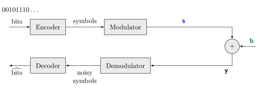
(a) Traditional communication scheme with no specific block for interference mitigation.

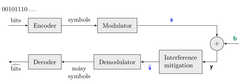
(b) Communication scheme with a dedicated building block for interference mitigation.

Figure 1: Communication schemes considered in this work.

We consider the point-to-point, single-channel, baseband signal model depicted in Fig. 1, where a transmitter aims to communicate a signal that carries a stream of encoded and modulated bits, referred to as the SOI and denoted as $\bm{\mathsf{s}}$. The signal is measured at the intended receiver in the presence of an unknown interference signal, denoted as $\bm{\mathsf{b}}$. The ultimate goal of the receiver is to successfully detect (or recover) the transmitted bits (or message) with the highest possible reliability, measured by the BER.

The input-output relation for a received, sampled, discrete-time baseband signal of length $N$ samples is given by

$$\bm{\mathsf{y}}=\bm{\mathsf{s}}+\bm{\mathsf{b}}\;\in\mathbb{C}^{N\times 1}.$$ (1)

This simplified model allows us to focus solely on the problem of interference rejection and the potential contributions of ML in this context. One can consider this model as the resulting input-output relation after successfully completing crucial processing stages in a communication system, such as time synchronization, channel estimation, and equalization. Although these aspects are deferred for future research, we acknowledge their importance in ensuring the correct operation of any practical communication system. Nonetheless, as we shall demonstrate throughout this paper, studying this building block in isolation enables us to understand the potential impact and challenges of integrating AI capabilities into RF communication receivers.

Furthermore, we consider the case where the generation process of the interference signal $\bm{\mathsf{b}}$ is unknown. Specifically, we assume that the interference consists of an unknown RF signal originating from another system operating in the same time-frequency band, possibly contaminated by AWGN.

Recall that we focus on digital communication signals as SOI in this work. In digital communication systems, the ultimate goal is to reliably recover the transmitted bits (or messages). Therefore, we consider the BER as a central measure of performance in this paper.

Note that we consider a scenario with non-Gaussian interference of unknown generation process, for which the optimal solution to minimize the BER is generally unknown. Under this setting, various receiver architectural designs can be devised based on different principles, aiming to achieve the best possible BER performance. In this work, we propose a hybrid, ”smart” receiver that first performs interference mitigation in a data-driven manner using a DNN. This approach aims to learn the relevant features of the unknown interference signal in order to mitigate it, and then, by treating the residual interference as Gaussian, apply standard matched filtering prior to decoding, so as to increase the postprocessing SNR. Consequently, we introduce a second measure of performance, namely the MSE between the estimated SOI $\hat{\mathbf{s}}$ and the true transmitted SOI $\bm{\mathsf{s}}$, to assess the signal quality after interference rejection and before decoding.

2.A SIGNAL MODELS

In this section, we categorize the various types of signals considered in this work based on our knowledge of their generation process.

When the signal’s generation process is known, we have detailed information about the generated signal. Specifically, we can generate a synthetic dataset of signals for the sake of learning a data-driven source separation module. This approach is valuable when model-based solutions are infeasible, either because the model of the interference is unknown (but the SOI’s model is known) or because the signal models are analytically intractable or computationally impractical. We will further categorize signals with a known generation process into single-carrier and multi-carrier signals.

When the signal generation process is unknown, we assume that we have datasets available, obtained through recordings or high-fidelity simulations. Thus, any knowledge relevant to performing source separation on these types of signals must be learned from the data.

2.A.1 SIGNALS WITH A KNOWN GENERATION PROCESS

We consider single-carrier and multi-carrier signals generated by linearly modulating symbols from constellations in the complex plane. Signals generated in this manner correspond to a prevalent class of digital communication signals observed in typical RF frequency bands.

Single-Carrier Signals

We consider single-carrier signals bearing $M$-bit long messages, which are mapped to $L$ symbols from a given complex constellation (e.g., quadrature phase shift keying (QPSK)) using Gray coding. The bits are randomly generated via a fair coin toss and are all independent and identically distributed (i.i.d.). The $n$-th sample of $\bm{\mathsf{s}}\in\mathbb{C}^{N\times 1}$ is expressed as

$$\mathsf{s}[n]=\sum_{\ell=0}^{L-1}\mathsf{a}_{\ell}\cdot g[n-\ell F-\tau_{0}],$$ (2)

where $\mathsf{a}_{\ell}\in\mathcal{A}$ denotes a complex discrete symbol to be transmitted, with $\mathcal{A}$ being the constellation (alphabet) of (possibly complex-valued) symbols, $F\in\use@mathgroup\M@U\symAMSb{Z}$ is the symbol interval (in discrete-time), $\tau_{0}\in\mathcal{S}_{0:F-1}$ is the offset for the first symbol, and $g[n]$ is the discrete-time impulse response of the transmitter filter (pulse shaping function). Fig. 2 shows a simplified diagram for the generation process of the considered single-carrier signal type.

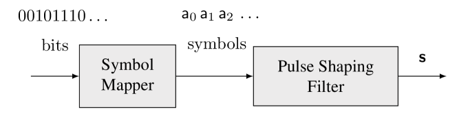
Figure 2: Block diagram for the generation process of the single-carrier signal, which modulates bits that are mapped into symbols from a complex-valued constellation before being filtered using a given pulse shaping filter.

Multi-Carrier Signals

For multi-carrier signals, we focus on orthogonal frequency-division multiplexing (OFDM) signals, one of the most common types used in key wireless communication technologies such as 5G and WiFi. An OFDM signal consists of $K$ orthogonal subcarriers, each carrying a symbol from a given complex constellation [20].

In this case as well, the bits are randomly generated using a fair coin toss in an i.i.d. manner and then mapped to symbols from the given constellation using Gray coding. The $n$-th sample of the SOI $\bm{\mathsf{s}}\in\mathbb{C}^{N\times 1}$ is given by

$$\mathsf{s}[n]=\sum_{p=0}^{P-1}\sum_{k=0}^{K-1}\mathsf{a}_{k,p}\,r[n-p\cdot(K+T_{\rm{cp}})-T_{\rm{cp}},\,k],$$ (3)

where

$$r[n,\,k]\triangleq\exp\left({j2\pi kn/K}\right)\cdot\mathbbm{1}_{\left\{-T_{\rm{cp}}\leq n<K\right\}}.$$ (4)

Here, $K$ represents the total number of orthogonal complex sinusoid terms (subcarriers), where not all of them are necessarily active. The value of $K$ corresponds to the fast Fourier transform (FFT) size of the inverse discrete Fourier transform (IDFT) involved in generating an OFDM signal. The coefficients $\mathsf{a}_{k,p}\in\mathcal{A}$ are the information modulating symbols, where $\mathcal{A}$ represents the alphabet (constellation). A cyclic prefix (CP) is typically added before an OFDM symbol. Thus, each OFDM symbol is described within the interval $[-T_{\rm{cp}},K]$, where $T_{\rm{cp}}$ is the CP length. The signals then span $P=N/(\bar{K}+T_{\rm{cp}})\in\use@mathgroup\M@U\symAMSb{Z}$ OFDM symbols, and their individual finite support is reflected by the finitely-supported function $r[n,k]$ in (4). Fig. 3 illustrates the block diagram of the OFDM symbol generation process.

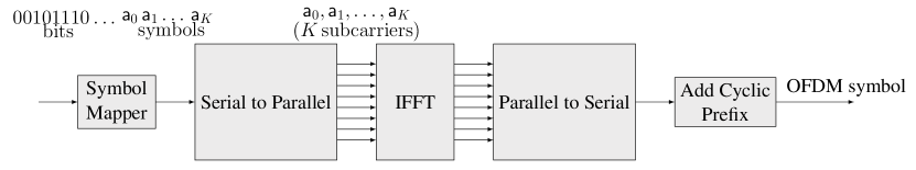
Figure 3: Block diagram for the generation process of an OFDM symbol carrying symbols in each active subcarrier.

2.A.2 SIGNALS WITH UNKNOWN GENERATION PROCESS

When dealing with unknown interference (e.g., from a different technology), accessing the signal generation process, which could potentially allow for the design of specific interference rejectors, is often rare. However, one can rely on recorded interference signals to learn how to design the interference rejector from the data. Another scenario where we may lack access to the generation process but still need to separate signals is the classical blind source separation problem. In this case, we may not know any of the signal models involved in the communication process, and our goal is simply to separate the superimposed signals into their constituent components. Finally, we could also consider the case where the generation process of the signals is known but too is complicated for deriving analytical solutions.

In any of these cases, the availability of signal datasets enables the design of data-driven source separators, thus providing an alternative to these classical approaches. We note that within the RF Challenge, there is a dataset of interference signals whose generative models are unknown, which can be used to develop learned, data-driven solutions.

The collection of datasets of relevant RF communication signals is therefore an essential component in the development of data-driven algorithmic solutions in the context of wireless communications. Although this work focuses on interference rejection problems, these signal datasets could be utilized for other purposes, importantly, for advancing solutions to various other issues associated with communication systems. We will further discuss this in Section 5.

3 METHODS

In this section, we review the methods used to perform interference mitigation over the various combinations of SOIs and interference signals considered in this work. Recall that in this work, the signal models are not necessarily known. Therefore, it is impossible to derive theoretical bounds on the performance metric of interest. For this reason, it is crucial that the set of numerically evaluated methods includes—alongside the novel, data-driven ones—traditional methods that are commonly used both in the literature and in practical communication systems, which are suitable and widely acceptable for benchmarking purposes.

3.A TRADITIONAL METHODS

We now present two prevalent methods whose appeal comes from the balance between their theoretical justification—and, in fact, optimality for common criteria under certain conditions—and their simplicity, an important virtue in practical systems.

3.A.1 LINEAR MMSE ESTIMATION

A computationally attractive approach that exploits the joint second-order statistics of the mixture (1) and the SOI is optimal minimum mean-square error (MMSE) linear estimation. Assuming $\det(\mathbf{C}_{\mathsf{y}\mathsf{y}})\neq 0$, the so-called linear minimum mean-square error (LMMSE) estimator [21], given by

$$\widehat{\bm{\mathsf{s}}}_{\text{\tiny LMMSE}}\triangleq\mathbf{C}_{\mathsf{s}\mathsf{y}}\mathbf{C}_{\mathsf{y}\mathsf{y}}^{-1}\bm{\mathsf{y}}=\mathbf{C}_{\mathsf{s}\mathsf{s}}\left(\mathbf{C}_{\mathsf{s}\mathsf{s}}+\mathbf{C}_{\mathsf{b}\mathsf{b}}\right)^{-1}\bm{\mathsf{y}}\in\use@mathgroup\M@U\symAMSb{C}^{N\times 1},$$ (5)

is constructed using the second-order statistics of the mixture that inherently take into account the potentially nontrivial temporal structure of the interference expressed through $\mathbf{C}_{\mathsf{b}\mathsf{b}}$. In other words, if $\mathbf{C}_{\mathsf{b}\mathsf{b}}$ somehow deviates from a scaled identity matrix, temporal cross-correlations exist.

While (5) coincides with the MMSE estimator when $\bm{\mathsf{y}}$ and $\bm{\mathsf{b}}$ are jointly Gaussian, it is generally suboptimal due to the linearity constraint. In our case, the signal $\mathsf{s}[n]$ is a digital communication signal and is certainly not Gaussian. As for $\mathsf{b}[n]$, its statistical model is assumed to be unknown throughout the design process of the interference mitigation module. Still, it would also typically be non-Gaussian, even if it contains AWGN, which is highly plausible.

Despite (5) not being the MMSE estimator in our scenarios of interest, it is still an important benchmark since it constitutes an attractive method for two main reasons. First, it is linear, and therefore fast and easy to implement for moderate values of $N$. Second, it only requires knowledge of second-order statistics, which are relatively easy to accurately estimate from data, even in real-time systems. We therefore use it as one of our benchmarks whenever it is computationally feasible.

3.A.2 MATCHED FILTERING

Matched filtering (MF), perhaps one of the most commonly used techniques in the signal processing chain of communication systems, exploits prior knowledge about the signal waveform (only) for enhanced detection of the transmitted symbols. When the residual (additive) component is Gaussian, it is optimal in the sense that it maximizes the SNR, and it is therefore also optimal in terms of minimum BER.

If the transmitted signal is represented by $\mathsf{s}[n]=\mathsf{a}_{0}\cdot g[n]$, where $g[n]$ is the pulse shaping filter, then the matched filter would be $h_{\text{\tiny MF}}[n]=g^{*}[-n]$. In practical scenarios, the pulse $g[n]$ has finite duration. After performing the complex conjugation and time-reversal to obtain $g^{*}[-n]$, the resulting signal is shifted appropriately to ensure causality. This shift corresponds to aligning the start of the pulse with the beginning of the observation window.

This method is also an important benchmark as it is probably still the most commonly used method for symbol detection, which is the natural choice when the residual component, be it noise or interference, is treated as AWGN.

To conclude this section, we note in passing that the (theoretically naïve) option of not applying an interference mitigation method will also be considered in our simulation as a benchmark. Indeed, with the complete absence of prior knowledge of the statistical model of the interference, this plain option of simply ignoring the interference may, after all, be chosen for practical considerations. While we do not advocate for such a solution approach, we acknowledge it as a realistic (even if not a leading) benchmark.

3.B DATA-DRIVEN METHODS

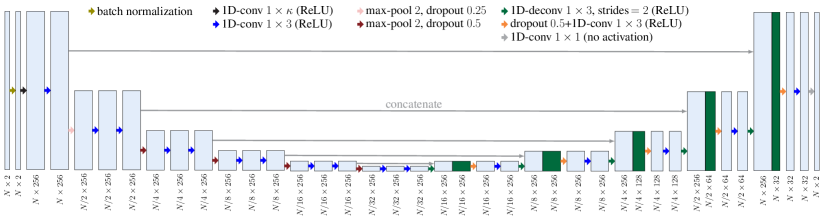
Figure 4: Architecture of the UNet DNN proposed to perform single-channel source separation of the communication signals. The parameter $\kappa$ denotes the kernel size of the first layer.

This section presents the two most powerful architectures we found for performing data-driven source separation of RF signals: the UNet and the WaveNet. We henceforth assume we have a dataset of $D$ i.i.d. copies of $\{(\bm{\mathsf{y}}^{(i)},\bm{\mathsf{s}}^{(i)})\}_{i=1}^{D}$.

3.B.1 UNET

The UNet, as depicted in Fig. 4, is a type of DNN originally proposed for biomedical image segmentation [22]. Its versatility has led to its adoption in various other applications, including spectrogram-based RF interference cancellation [23] and audio source separation [10, 24]. These applications typically correspond to a multivariate regression setup with identical dimensions for both input and output data.

Similarly to these aforementioned works, our approach employs 1D-convolutional layers to better capture the temporal features of time-series data. To effectively handle (baseband) complex-valued signals, inspired by widely linear estimation techniques [25], we represent the real and imaginary parts as separate input channels. The UNet architecture comprises downsampling blocks, which operate on progressively coarser timescales, and incorporates skip connections to combine features from different timescales with the upsampling blocks.

It is well known that a careful design of the neural network architecture, motivated by the specific application at hand, can significantly impact performance, as demonstrated in our experiments and architectural choices. Specifically, unlike standard CNN-based architectures tailored for image processing, which typically employ short kernels of size $\sim 3$ in all layers, our UNet architecture features a first convolutional layer with a nonstandard, comparatively long kernel (indicated by $\kappa$ in Fig. 4), which can be of size $\sim 100$—a difference of two orders of magnitude. We observed that proper adjustment of this parameter to capture the effective correlation length of both the SOI and interference facilitates (and perhaps enables, as some of our findings indicates) the extraction of additional long-scale temporal structures of both signals, leading to performance gains of an order of magnitude compared to the originally proposed UNet [22].

3.B.2 WaveNet

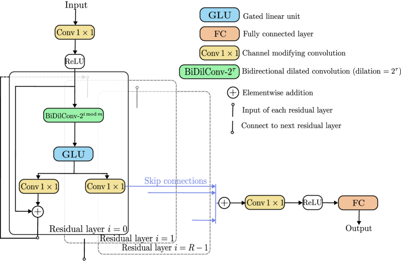
Figure 5: Architecture of the WaveNet DNN proposed to perform single-channel source separation of the communication signals.

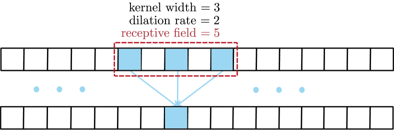
Figure 6: A dilated convolution operation with a kernel width of $3$ and a dilation rate of $2$, which results in a receptive field of $5$.

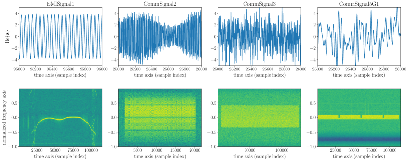
Figure 7: Representative frames of the four interference signal types in the dataset: EMISignal1, CommSignal2, CommSignal3, and CommSignal5G1. Top: Real part of the waveforms, $\mathrm{Re}\{\mathbf{s}\}$; Bottom: Spectrogram of the respective signal frames.

The WaveNet architecture [26] was initially introduced as a generative neural network for synthesizing raw audio waveforms. At its core, the architecture uses stacked layers of convolutions with gated activation units. Unlike the downsampling and upsampling networks used in UNets, WaveNet preserves the temporal resolution at each hidden layer by leveraging dilated convolutions. As shown in Fig. 6, the dilated convolution can be interpreted as a “virtual” kernel with spacing between elements, enlarging the effective receptive field of the convolution. For example, a dilated convolution with a kernel width of 3 and a dilation of 2 has an effective receptive field of 5.

As illustrated in Fig. 5, the WaveNet employs $R$ residual blocks with dilated convolutions, where the output of block $i-1$ serves as the input to block $i$, for $i\in\{0,\dots,R-1\}$. The dilated convolutions assist in learning long-range temporal and periodic structures. The dilations start small and successively increase, such that the dilation at block $i$ is given by $2^{i\,\textrm{mod}\,m}$, where $m$ is the dilation cycle length. For example, if the dilation periodicity is $m=10$, then in block $i=9$ the dilation is 512, and in block $10$ the dilation is reset to 1. This allows the network to efficiently trade off between learning local and global temporal structures. All residual blocks use the same number of channels, $C$. Our WaveNet specifically uses $R=30$ residual blocks, with a dilation cycle $m=10$, and a number of channels per residual block of $C=128$.

Several modifications were made to facilitate training with RF signals compared to the original WaveNet [26]. First, since we are dealing with complex-valued continuous waveforms, we train on two-channel signals where the real and imaginary components of the RF signals are concatenated in the channel dimension. Second, we train with an MSE (squared $\ell_{2}$) loss, as we did with the UNet. We monitor the validation MSE loss, and once the loss stops decreasing substantially, we stop training early. Lastly, we increased the channel dimension up to $C=128$ to learn complex RF signals such as OFDM signals. Additionally, during data loading, we perform random time shifts and phase rotations on the SOIs to gain diversity and simulate typical transmission impairments in RF systems.

4 RF CHALLENGE RESULTS

We now present a diverse set of results for RF signal separation. We consider different types of mixtures, involving various combinations of signal types, which result in different underlying joint statistical characteristics. This leads to varying levels of difficulty in learning optimal separation operators, or even finding “good” separators that outperform the best computationally feasible methods available today. We compare the performance of several approaches, including data-driven, neural network-based separators, as well as more traditional, commonly used methods. Beyond showcasing our contributions in developing ML-enhanced RF signal separation architectures, it is crucial to establish standardized benchmarks that will serve as baselines for future research in this emerging field.

To analyze decoding capabilities (in terms of BER) alongside interference rejection capabilities (in terms of the MSE of the “denoised” SOI), we consider SOIs with known generative processes in this work. Specifically, we consider two different SOIs and four types of interference, resulting in eight different combinations of mixture types, each of length $N=40,960$ samples.

For the SOIs, we have:

1. QPSK: A single-carrier QPSK signal with an oversampling factor of $F=16$, modulated by a root-raised cosine pulse shaping function with a roll-off factor of $0.5$ that spans $128$ samples ($8$ QPSK symbols due to the employed oversampling factor). We further apply an offset for the first symbol of $\tau_{0}=8$ samples. See Fig. 2 for a simplified diagram of the generation process of this SOI. We refer to this signal simply as “QPSK”.

2. OFDM-QPSK: An OFDM signal where each subcarrier bears a QPSK symbol. We refer to this signal as “OFDM-QPSK”. We set $T_{\rm{cp}}=16$, $K=64$ subcarriers, and $\bar{K}=56$ active subcarriers (i.e., the $8$ inactive subcarriers “carry” the zero symbol), referring to the quantities in (3). A simplified diagram of the generation process of this SOI is shown in Fig. 3.

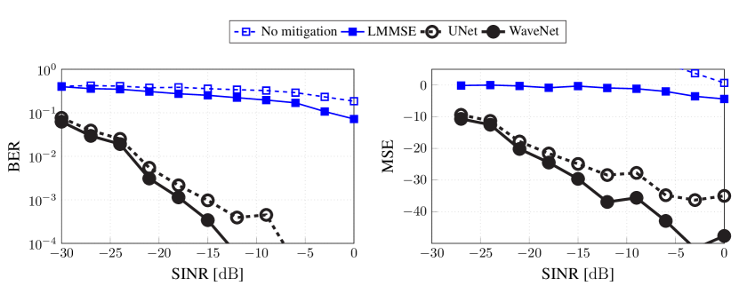
(a) EMISignal1 interference.

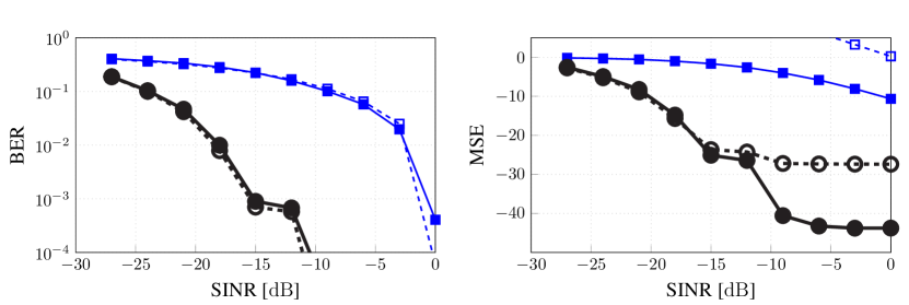
(b) Commsignal2 interference.

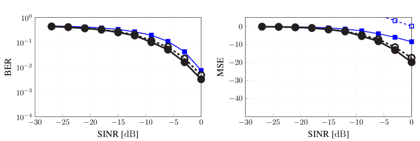
(c) Commsignal3 interference.

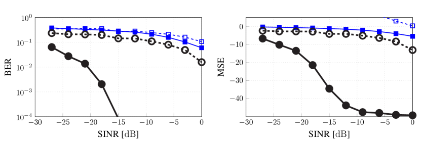
(d) Commsignal5G1 interference.

Figure 8: BER and MSE as a function of the target SINR for all combinations of QPSK SOI and the different interference types considered in this work.

The four types of interference signals are only available through provided recordings, hence their generation process is unknown:

1. EMISignal1: Electromagnetic interference from unintentional radiation from a man-made source.

2. CommSignal2: A digital communication signal from a commercially available wireless device.

3. CommSignal3: Another digital communication signal from a commercially available wireless device.

4. CommSignal5G1: A 5G-compliant waveform.

We emphasize that the generative processes of the signals above are not only considered unknown in the simulations, but are in fact truely unknown to the authors. The dataset examples for the first three types (EMISignal1, CommSignal2, and CommSignal3) were recorded over-the-air, while the last one (CommSignal5G1) was generated and recorded within a controlled wired laboratory environment, with wireless impairments introduced via simulators.

To create interference signal examples, a frame of the respective interference type was selected at random (uniformly) from the dataset, and a random window of $N=40,960$ samples was extracted. Each interference component was scaled to achieve a target (empirical) signal-to-interference-and-noise ratio (SINR). Since all signal datasets are normalized to have unit power, for a target SINR level $\kappa^{2}=10^{(\textrm{\lx@glossaries@gls@link{main}{sinr}{\leavevmode{\color[rgb]{0,0,0}SINR}} in dB})/10}$, the interference signal is scaled by $1/\kappa$. Each interference frame $\bm{\mathsf{b}}^{(i)}$ also undergoes a random phase rotation before being added to the SOI $\bm{\mathsf{s}}^{(i)}$ to create a mixture example $\bm{\mathsf{y}}^{(i)}$ (see (1)).

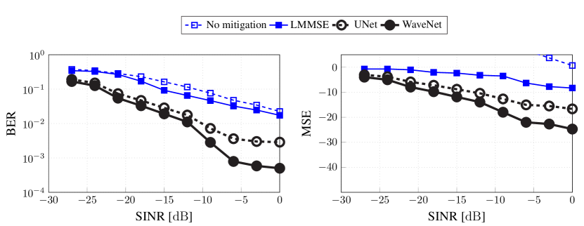
(a) EMISignal1 interference.

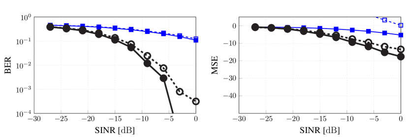
(b) Commsignal2 interference.

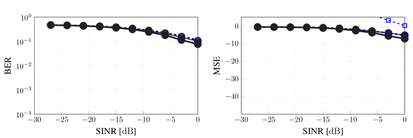
(c) Commsignal3 interference.

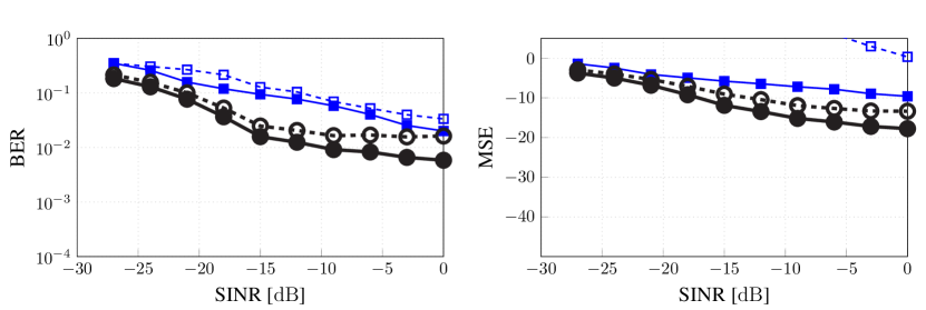
(d) Commsignal5G1 interference.

Figure 9: BER and MSE as a function of the target SINR for all combinations of OFDM-QPSK SOI and the different interference types considered in this work.

For the recorded interferences, while the length of each frame is consistent within a given signal type, it varies across types: $230,000$ samples for EMISignal1, $43,560$ for CommSignal2, $260,000$ for CommSignal3, and $230,000$ for CommSignal5G1. For consistency, we set the length of all input mixtures to $40,960$ samples. Signals EMISignal1 and CommSignal5G1 were shifted in frequency to have their spectral energy content lie in baseband frequencies, simulating co-channel interference that overlaps both in time and frequency. Fig. 7 shows the time- and frequency-domain representations of the recorded signal datasets used as interferences. More details and code examples can be found at https://rfchallenge.mit.edu/icassp24-single-channel/.

4.A OUR RESULTS

Figures 8 and 9 show the performance of the two traditional interference rejection algorithms, introduced in Section 3.A, and our proposed deep learning-based interference rejection algorithms, introduced in Section 3.B, over the eight possible SOI-interference combinations. The performance is measured in terms of BER or MSE as a function of the target SINR. All plots include the following curves:

• LMMSE: the SOI is estimated via MSE-optimal linear estimation, the best-performing traditional method described in Section 3.A.

• UNet and WaveNet: the architectures we developed, presented in Section 3.B.

Both learning-based solutions described in Section 3.B outperform the best traditional method based on LMMSE estimation, achieving up to two orders of magnitude performance improvements at considerably low SINR values. For instance, in Fig. 8(d), at an SINR value of $-18\,\mathrm{dB}$, the WaveNet model achieves a BER of approximately $10^{-3}$ and an MSE below $-20\,\mathrm{dB}$. In contrast, the solutions based on LMMSE and no mitigation only reach a BER slightly above $10^{-1}$ and an MSE around $0~{}\mathrm{dB}$.

4.B COMPETITION RESULTS

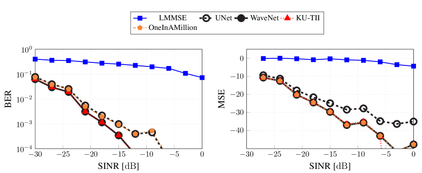
(a) EMISignal1 interference.

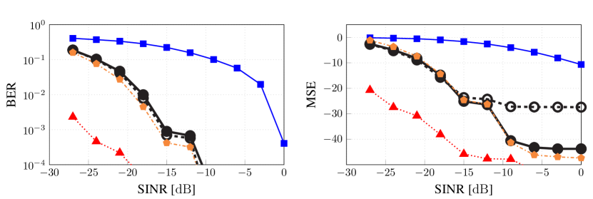
(b) Commsignal2 interference.

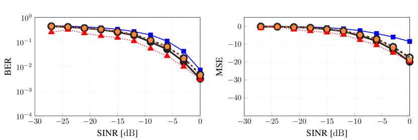
(c) Commsignal3 interference.

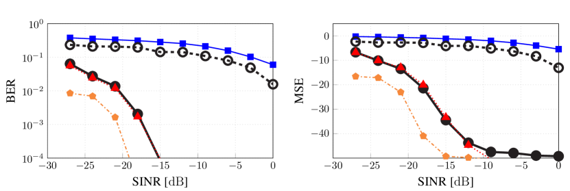
(d) Commsignal5G1 interference.

Figure 10: BER and MSE as a function of the target SINR for all combinations of QPSK SOI and the different interference types considered in this work.

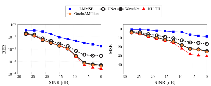
(a) EMISignal1 interference.

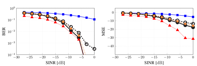
(b) Commsignal2 interference.

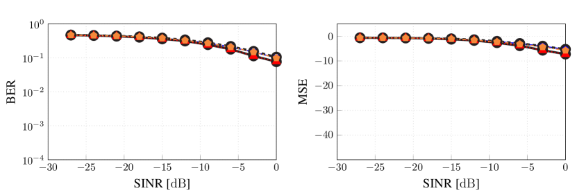
(c) Commsignal3 interference.

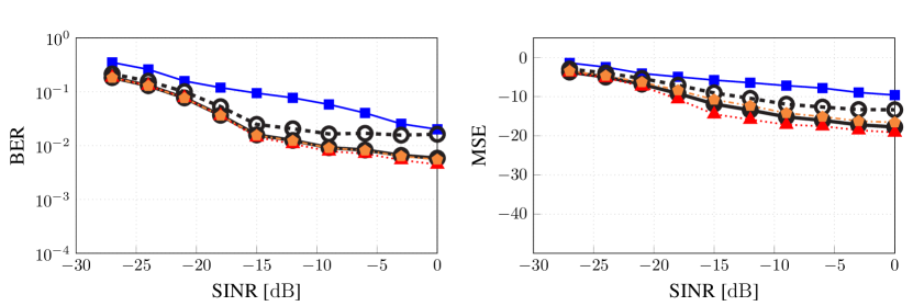
(d) Commsignal5G1 interference.

Figure 11: BER and MSE as a function of the target SINR for all combinations of OFDM-QPSK SOI and the different interference types considered in this work.

We recently hosted the “Data-Driven Radio Frequency Signal Separation Challenge” as one of the ICASSP’24 signal processing grand challenges [19]. Among the received submissions, only a few outperform the learning-based methods described in Section 3.B [27, 28]. Similar to the previous section, Figures 10 and 11 show the performance of the traditional interference rejection algorithm based on LMMSE estimation, our proposed deep learning-based interference rejection algorithms introduced in Section 3.B, and the two top-performing teams that participated in the challenge. We only include these two teams as they were the only ones that could improve significantly upon our reference methods at least at one signal mixture case out of the eight possible SOI-interference combinations. Complete results including all participant submissions can be found at https://rfchallenge.mit.edu/icassp24-single-channel/.

As we can see, these two teams improved upon the baselines in some cases involving EMISignal1, CommSignal2, and CommSignal5G1 (see Figs. 10(b), 10(d), 11(a), and 11(b)). For example, “KU-TII” [27] especially shines in those mixture involving CommSignal2 interference, where they gain more than an order of magnitude in BER at SINR values below $-20\,{\rm dB}$ compare to our baseline architectures, and “OneInAMillion” [28] performs especially well in the QPSK + CommSignal5G mixture, where they almost achieved an order of magnitude gain in BER at SINR values below $-20\,{\rm dB}$. Conversely, mixtures with CommSignal3 consistently challenge all methods. While we believe it is a multicarrier signal with a high data rate, the specific reasons for the difficutly to separate CommSignal3 from the SOI remain unclear, warranting further investigation.

These results show the potential of data-driven, deep-learning-based solutions to provide significant improvements in interference rejection tasks when the interference presents unknown structures that can be learned. They also demonstrate that the baseline solutions we developed (presented in Section 3.B) are robust and not easily outperformed, suggesting that innovative solutions are needed to achieve further performance gains, especially for challenging signals such as CommSignal3.

5 FUTURE DIRECTIONS AND CONCLUDING REMARKS

In this section, we explore potential future research directions that can further advance the field of data-driven source separation of RF signals using deep learning techniques. We also provide concluding remarks to encapsulate the key findings of this paper.

5.A FUTURE RESEARCH DIRECTIONS

This work demonstrates that data-driven deep learning algorithms for RF source separation can yield significant performance gains. However, in order to make these techniques practically relevant, further in-depth research of different aspect of the problem is necessary, giving rise to several promising avenues for future research. We believe these directions can facilitate the integration of such techniques into next-generation RF systems. Below, we outline some important areas for further development to achieve this goal.

SOIs with Unknown Generation Process

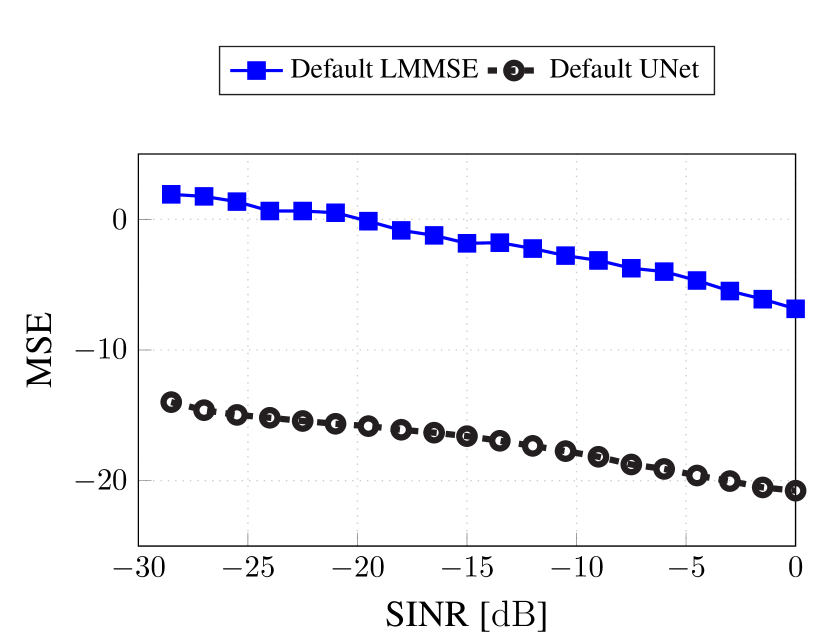
(a) EMISignal1 interference.

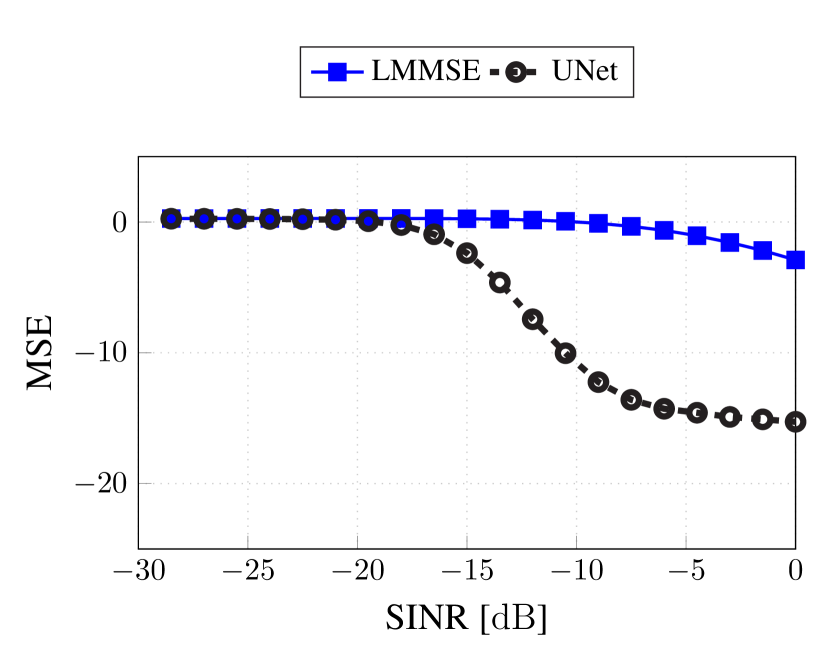
(b) Commsignal3 interference.

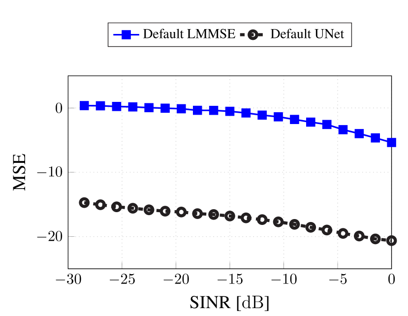
(c) Commsignal5G1 interference.

Figure 12: MSE as a function of the target SINR for all combinations of CommSignal2 SOI and the rest of interference types considered in this work.

A direct extension of this work is to investigate scenarios where the generation process of the SOI is unknown. Such cases are more challenging, as there is no additional information to exploit when designing the source separation algorithm. For example, in the results presented in Section 4, we leveraged knowledge of the modulation scheme of the SOI to improve performance, which we measured in terms of BER. However, when the signal generation process is unknown, this approach is not applicable.

We have conducted preliminary studies using CommSignal2 as the SOI, evaluating the MSE of the SOI reconstruction post-separation using the UNet architecture (Section 3.B.1) and traditional LMMSE estimation (Section 3.A). We used the remaining signals in the dataset as interference signals. The results, presented in Fig. 12, demonstrate that the UNet architecture outperforms LMMSE, except at low SINR levels when CommSignal3 acts as interference. This again highlights the need for further research into handling such intricate signal types that constitute bothersome interference.

Extension of Modulation Schemes

Expanding this work to include other types of modulation schemes with higher-order modulations (e.g., 16-QAM, 64-QAM) and other waveform designs can provide valuable insights. Higher-order modulations are commonly used in modern communication systems, such as Wi-Fi and 5G, to achieve higher data rates. Investigating the performance of source separation algorithms under these conditions will help in understanding their robustness and adaptability to various signal characteristics.

Additionally, exploring different modulation formats such as phase shift keying (QPSK) and frequency shift keying (FSK), as well as combinations of these, could uncover potential limitations or strengths of the current deep learning architectures. These modulation schemes are prevalent in various wireless technologies, including Bluetooth and Zigbee, which are integral to many consumer and industrial applications.

Examining modulation schemes and waveform designs specific to IoT technologies can be particularly insightful. For instance, LoRa employs chirp spread spectrum (CSS) [29], Sigfox uses Ultra Narrowband [30], and NB-IoT utilizes single-tone and multi-tone FSK [31]. These technologies have unique modulation requirements due to their focus on low power consumption and extended range. Understanding how source separation algorithms perform with these schemes can help in optimizing IoT communication systems and enhancing their reliability and efficiency.

MIMO Systems

Multiple-input multiple-output (MIMO) systems leverage spatial diversity by using multiple antennas at both the transmitter and receiver ends, significantly enhancing communication performance. Exploring how to exploit spatial structures in tandem with the signals’ unique (and learnable) statistical characteristics presents another promising avenue for future research.

Incorporating MIMO capabilities in source separation algorithms can lead to substantial performance improvements, particularly in terms of signal robustness and data throughput. MIMO systems are a cornerstone of modern wireless communication standards such as 5G and Wi-Fi, where they are utilized to increase capacity and spectral efficiency. In addition to traditional applications, MIMO systems are also finding use in emerging technologies such as vehicle-to-everything communications and industrial IoT. These applications often require robust and reliable communication in dynamic and interference-prone environments. Although the multi-channel source separation literature is significantly richer than the single-channel one(e.g., [32, 33, 34, 35]), understanding how modern data-driven deep-learning algorithms for source separation can be adapted to take advantage also of the spatial resolution in MIMO systems is crucial for their potential integration into these future technologies.

Synchronization and CSI Acquisition

The signal model addressed in the present work is a fairly accurate representation under the assumption of successful completion of key stages such as time synchronization, channel estimation, and equalization. However, these assumptions may not always hold, particularly in scenarios with persistent (i.e., not bursty) interference. To enhance the model’s applicability, a more generalized approach is needed.

A comprehensive, baseband, discrete-time system model should also incorporate effects such as arbitrary time shifts and fading effects. More generally, the input-output relationship of such an extended model can be expressed as:

$$\mathsf{y}[n]=\mathcal{H}\left\{\mathsf{s}[n]\right\}+\mathsf{b}[n-\mathsf{k}_{b}],\,\,n\in\use@mathgroup\M@U\symAMSb{Z},$$ (6)

where $\mathsf{s}[n]$ and $\mathsf{b}[n]$ are the SOI and interference, respectively, and $\mathcal{H}\{\cdot\}$ denotes the channel response. For example, the channel could be $\mathcal{H}\left\{\mathsf{s}[n]\right\}=\alpha\cdot\mathsf{s}[n-\mathsf{k}_{s}]$ for some fading coefficient $\alpha\in\use@mathgroup\M@U\symAMSb{C}$ and an unknow delay $\mathsf{k}_{s}\in\mathbb{N}$. Note that $\mathcal{H}\{\cdot\}$ is not necessarily linear, not time-invariant. The advantage (and beauty) of the data-driven approach is that it can potentially learn to compensate for nonlinear, time-varying effects, provided they are well captured in the available signal datasets for training.

The parameters $\mathsf{k}_{s}$ and $\mathsf{k}_{b}$, both integers in the example above of the generalized discrete-time model, represent arbitrary time-shifts relative to a reference point within the signal. Communication signals often exhibit cyclostationary characteristics, implying that $\mathsf{s}[n]$ and $\mathsf{b}[n]$ can be viewed as cyclostationary processes with known fundamental cyclic periods $K_{s}$ and $K_{b}$, respectively. If we model the signals as cyclostationary, one could consider the parameters $\mathsf{k}_{s}$ and $\mathsf{k}_{b}$ as discrete time-shifts concerning the start of the cyclic period of each signal, typically chosen arbitrarily as $n=0$ for convenience. Consequently, one might assume distributions such as $\mathsf{k}_{s}\sim{\rm Unif}\left(\mathcal{S}_{K_{s}}\right)$ and $\mathsf{k}_{b}\sim{\rm Unif}\left(\mathcal{S}_{K_{b}}\right)$ to represent the variability of these parameters [36].

It is also worth noting that wireless fading channels can be statistically modeled as well, which usually allow for tractable mathematical analyses. For instance, the quasi-static fading channel maintains a constant fading coefficient throughout the transmission, whereas the block-fading channel preserves this constancy within a coherence interval before changing independently and identically across successive intervals. The choice of a specific model depends on the application’s requirements [37, Ch. 5]. Efficient channel state information (CSI) acquisition, with the ultimate goal of performing interference rejection, presents an interesting research topic.

An RF Signal Separation “Foundation-like” Model

The data-driven solutions presented in this work are all ones that were specifically tailored for a given type of mixture, namely a mixture of a specific SOI type and a specific interference type. While this is clearly statistically preferable (i.e., a model trained for each mixture type), it generally implies a high demand of resources from a system perspective (e.g., memory—a NN for every possible received mixture). In this respect, it would be attractive to obtain a single model that can mitigate several types of interference. Such a model can be viewed as a (“micro”) instance of an RF foundation model [38, 39], where the different signal types (i.e., codes, modulations, pulse shaping functions, etc.) are viewed as the different “modalities”. One of the first steps towards such a powerful architecture is to show (both theoretically and empirically) that it is indeed possible to have a single model that can cope with a few types of intereference signals, while attaining the same performance (in terms of inference time and signal reconstruction accuracy) as the individually trained ones.

Real-Time Operation and Computational Efficiency

One of the main challenges in integrating deep learning techniques into RF systems is ensuring real-time operation while maintaining computational efficiency. The computational complexity and energy consumption of deep learning models pose significant hurdles for practical implementation in communication standards (e.g., [40]). Therefore, developing efficient algorithms with a clear understanding of their computational costs is crucial.

Efforts in this direction include the design of low-complexity schemes capable of competing with architectures optimized for performance. Additionally, examining the computational complexity and resource requirements of algorithms when dealing with higher-order and more complex modulation schemes is essential. This assessment is particularly vital for practical implementations, especially in resource-constrained environments like IoT devices and mobile communications.

Ensuring that the proposed methods are not only effective but also efficient will be key to their adoption in next-generation RF systems.

5.B CONCLUDING REMARKS

This paper, using the RF Challenge developments, illustrates the promising potential of deep learning-based algorithms for source separation of RF signals. Specifically, we show that mitigating strong unintentional interference from other systems utilizing the same time-frequency resources with data-driven methods leads to considerable gains relative to conservative methods. Through extensive simulations encompassing eight different signal mixtures, we have demonstrated the superior performance of deep learning architectures such as UNet and WaveNet over traditional signal processing methods like matched filtering and LMMSE estimation across various scenarios. However, results from different leading research teams that participated in the RF Challenge show that this is not a straightforward problem and that surpassing the established deep-learning benchmarks is not an easy task, especially in mixtures involving multi-carrier signals.

Ultimately, the results described herein represent merely an initial phase of a more extensive journey towards integrating AI capabilities into receivers for enhanced interference rejection. The path forward will involve addressing intermediate challenges and presenting viable solutions to demonstrate the tangible benefits of these approaches. Indeed, the results motivate further research and development for this dynamic domain within the broader community, with the ultimate goal of significantly improving future generations of RF systems spanning diverse applications.

References

- [1] Qualcomm Technologies Inc., “VR and AR pushing connectivity limits,” https://www.qualcomm.com/content/dam/qcomm-martech/dm-assets/documents/presentation_-_vr_and_ar_are_pushing_connectivity_limits_-web_0.pdf, Accessed: 2024-02-26.
- [2] Mohammed Hirzallah, Wessam Afifi, and Marwan Krunz, “Full-duplex-based rate/mode adaptation strategies for Wi-Fi/LTE-U coexistence: A POMDP approach,” IEEE J. Sel. Areas Commun., vol. 35, no. 1, pp. 20–29, Nov. 2017.
- [3] Gaurang Naik, Jung-Min Park, Jonathan Ashdown, and William Lehr, “Next generation Wi-Fi and 5G NR-U in the 6 GHz bands: Opportunities and challenges,” IEEE Access, vol. 8, pp. 153027–153056, Aug. 2020.
- [4] T. Oyedare, V. K. Shah, D. J. Jakubisin, and J. H. Reed, “Interference suppression using deep learning: Current approaches and open challenges,” IEEE Access, 2022.
- [5] Harry L. Van Trees, Detection, Estimation, and Modulation Theory, Part I:, Wiley, New York, NY, USA, 2001.
- [6] Tu Shilong, Chen Shaohe, Zheng Hui, and Wan Jian, “Particle filtering based single-channel blind separation of co-frequency MPSK signals,” in IEEE Int. Symp. Intell. Signal Process. and Commun. Syst., Feb. 2007, pp. 582–585.
- [7] Tu Shilong, Zheng Hui, and Gu Na, “Single-channel blind separation of two QPSK signals using per-survivor processing,” in IEEE Asia Pac. Conf. Circuits Syst. (APCCAS), Dec. 2008, pp. 473–476.
- [8] Timothy J. O’shea and Nathan West, “Radio machine learning dataset generation with GNU radio,” in Proc. GNU Radio Conf., 2016, vol. 1.
- [9] MIT RLE, “RF Challenge - AI Accelerator,” Accessed 2024-02-26.
- [10] D. Stoller, S. Ewert, and S. Dixon, “Wave-U-Net: A multi-scale neural network for end-to-end audio source separation,” in Intl. Soc. for Music Inf. Retrieval Conf., May 2018, pp. 334–340.
- [11] Aditya Arie Nugraha, Antoine Liutkus, and Emmanuel Vincent, “Multichannel audio source separation with deep neural networks,” IEEE/ACM Trans. Audio, Speech, Lang. Process., vol. 24, no. 9, pp. 1652–1664, June 2016.
- [12] Yosef Gandelsman, Assaf Shocher, and Michal Irani, ““Double-DIP”: Unsupervised image decomposition via coupled deep-image-priors,” in Proc. of IEEE/CVF Conf. Comput. Vis. Pattern Recognit. (CVPR), June 2019, pp. 11026–11035.
- [13] Po-Sen Huang, Minje Kim, Mark Hasegawa-Johnson, and Paris Smaragdis, “Joint optimization of masks and deep recurrent neural networks for monaural source separation,” IEEE/ACM Trans. Audio, Speech, Lang. Process., vol. 23, no. 12, pp. 2136–2147, Dec. 2015.
- [14] Taiwo Remilekun Oyedare, “A comprehensive analysis of deep learning for interference suppression, sample and model complexity in wireless systems,” 2024.
- [15] DeepSig Inc., “RF Datasets For Machine Learning,” Accessed 2024-02-20.
- [16] IQ Engine, “A web-based SDR toolkit for analyzing, processing, and sharing RF recordings,” Accessed 2024-02-26.
- [17] G. C. F. Lee, A. Weiss, A. Lancho, J. Tang, Y. Bu, Y. Polyanskiy, and G. W. Wornell, “Exploiting temporal structures of cyclostationary signals for data-driven single-channel source separation,” in IEEE Int. Workshop Mach. Learn. Signal Process., Aug. 2022.
- [18] T. Jayashankar, G. C. F. Lee, A. Lancho, A. Weiss, Y. Polyanskiy, and G. W. Wornell, “Score-based source separation with applications to digital communication signals,” in Advances Neural Inform. Proc. Syst. (NeurIPS), New Orleans, LA, 2023.
- [19] Tejas Jayashankar, Benoy Kurien, Alejandro Lancho, Gary C.F. Lee, Yury Polyanskiy, Amir Weiss, and Gregory Wornell, “The data-driven radio frequency signal separation challenge,” in To appear in Proc. IEEE Int. Conf. Acoust., Speech, Signal Process. (ICASSP), April 2024.
- [20] Taewon Hwang, Chenyang Yang, Gang Wu, Shaoqian Li, and Geoffrey Ye Li, “OFDM and its wireless applications: A survey,” IEEE Trans. Veh. Technol., vol. 58, no. 4, pp. 1673–1694, 2008.
- [21] Harry L. Van Trees, Detection, Estimation, and Modulation Theory, Part I: Detection, Estimation, and Linear Modulation Theory, John Wiley & Sons, 2004.
- [22] O. Ronneberger, P. Fischer, and T. Brox, “U-Net: Convolutional networks for biomedical image segmentation,” in Med. Image Comput. Comput. Assist. Interv. 2015, pp. 234–241, Springer.
- [23] Joel Akeret, Chihway Chang, Aurelien Lucchi, and Alexandre Refregier, “Radio frequency interference mitigation using deep convolutional neural networks,” arXiv:1609.09077, 2017.
- [24] Efthymios Tzinis, Zhepei Wang, and Paris Smaragdis, “Sudo RM-RF: Efficient networks for universal audio source separation,” in Proc. of MLSP, 2020, pp. 1–6.
- [25] Bernard Picinbono and Pascal Chevalier, “Widely linear estimation with complex data,” IEEE Trans. Signal Process., vol. 43, no. 8, pp. 2030–2033, 1995.
- [26] Aäron van den Oord, Sander Dieleman, Heiga Zen, Karen Simonyan, Oriol Vinyals, Alex Graves, Nal Kalchbrenner, Andrew W. Senior, and Koray Kavukcuoglu, “Wavenet: A generative model for raw audio,” CoRR, vol. abs/1609.03499, 2016.
- [27] Yu Tian, Ahmed Alhammadi, Abdullah Quran, and Abubakar Sani Ali, “A novel approach to wavenet architecture for rf signal separation with learnable dilation and data augmentation,” in 2024 IEEE International Conference on Acoustics, Speech, and Signal Processing Workshops (ICASSPW), Apr. 2024, pp. 79–80.
- [28] Fadli Damara, Zoran Utkovski, and Slawomir Stanczak, “Signal separation in radio spectrum using self-attention mechanism,” in 2024 IEEE International Conference on Acoustics, Speech, and Signal Processing Workshops (ICASSPW), Apr. 2024, pp. 99–100.
- [29] Jothi Prasanna Shanmuga Sundaram, Wan Du, and Zhiwei Zhao, “A survey on LoRa networking: Research problems, current solutions, and open issues,” IEEE Commun. Surveys Tuts., vol. 22, no. 1, pp. 371–388, 2019.
- [30] Alexandru Lavric, Adrian I Petrariu, and Valentin Popa, “Sigfox communication protocol: The new era of iot?,” in n Proc. Int. Conf. Sens. Instrum. IoT Era (ISSI), 2019, pp. 1–4.
- [31] Matthieu Kanj, Vincent Savaux, and Mathieu Le Guen, “A tutorial on nb-iot physical layer design,” IEEE Commun. Surveys Tuts., vol. 22, no. 4, pp. 2408–2446, 2020.
- [32] Aapo Hyvarinen, “Fast and robust fixed-point algorithms for independent component analysis,” IEEE Trans. Neural Netw., vol. 10, no. 3, pp. 626–634, 1999.
- [33] Adel Belouchrani, Karim Abed-Meraim, J-F Cardoso, and Eric Moulines, “A blind source separation technique using second-order statistics,” IEEE Trans. Signal Process., vol. 45, no. 2, pp. 434–444, 1997.
- [34] Arie Yeredor, “Non-orthogonal joint diagonalization in the least-squares sense with application in blind source separation,” IEEE Trans. Signal Process., vol. 50, no. 7, pp. 1545–1553, 2002.
- [35] Amir Weiss and Arie Yeredor, “A maximum likelihood-based minimum mean square error separation and estimation of stationary Gaussian sources from noisy mixtures,” IEEE Trans. Signal Process., vol. 67, no. 19, pp. 5032–5045, July 2019.
- [36] A. Lancho, A. Weiss, G. C. F. Lee, J. Tang, Y. Bu, Y. Polyanskiy, and G. W. Wornell, “Data-driven blind synchronization and interference rejection for digital communication signals,” in IEEE Glob. Commun. Conf. (GLOBECOM), Dec. 2022, pp. 2296–2302.
- [37] Andreas F. Molisch, Wireless Communications, Wiley Publishing, 2nd edition, 2011.
- [38] Rishi Bommasani, Drew A Hudson, Ehsan Adeli, Russ Altman, Simran Arora, Sydney von Arx, Michael S Bernstein, Jeannette Bohg, Antoine Bosselut, Emma Brunskill, et al., “On the opportunities and risks of foundation models,” arXiv:2108.07258, 2021.
- [39] Jaron Fontaine, Adnan Shahid, and Eli De Poorter, “Towards a wireless physical-layer foundation model: Challenges and strategies,” arXiv:2403.12065, Feb. 2024.
- [40] Tejas Jayashankar, Gary CF Lee, Alejandro Lancho, Amir Weiss, Yury Polyanskiy, and Gregory Wornell, “Score-based source separation with applications to digital communication signals,” Advances in Neural Information Processing Systems, vol. 36, 2024.