Angular Co-variance using intrinsic geometry of torus:
Non-parametric change points detection in meteorological data

Abstract.

In many temporal datasets, the parameters of the underlying distribution may change abruptly at unknown times. Detecting these changepoints is crucial for numerous applications. While this problem has been extensively studied for linear data, there has been remarkably less research on bivariate angular data. For the first time, we address the changepoint problem for the mean direction of toroidal and spherical data, which are types of bivariate angular data. By leveraging the intrinsic geometry of a curved torus, we introduce the concept of the “square” of an angle. This leads us to define the “curved dispersion matrix” for bivariate angular random variables, analogous to the dispersion matrix for bivariate linear random variables. Using this analogous measure of the “Mahalanobis distance,” we develop two new non-parametric tests to identify changes in the mean direction parameters for toroidal and spherical distributions. We derive the limiting distributions of the test statistics and evaluate their power surface and contours through extensive simulations. We also apply the proposed methods to detect changes in mean direction for hourly wind-wave direction measurements and the path of the cyclonic storm “Biporjoy,” which occurred between 6th and 19th June 2023 over the Arabian Sea, western coast of India.

1. Introduction

The presence of bivariate angular or directional data is very common in different disciplines of sciences, for example dihedral (torsion) angles in protein structures (bioinformatics), wind directions & sea wave directions (meteorology), the path of a cyclone (climatology), daily occurrence time of maximum and minimum share price of a stock (finance), etc. Such data refers to measurements that exhibit a circular or periodic nature. After a suitably chosen location of the origin, the data can be represented on a torus ($\mathbb{S}_{1}\times\mathbb{S}_{1}$) or the sphere $\mathbb{S}_{2}$ depending on the range of the data. For a comprehensive exploration of bivariate circular data, refer to Mardia et al. (2000) and Ley and Verdebout (2017).

Change point analysis is a key statistical technique used to detect unexpected shifts or changes in a data sequence over time. These changes can occur due to variations in the parameters within the same distribution family or a complete switch to a different distribution family. The presence of change points can significantly disrupt standard statistical analyses. Therefore, the main goal of change point analysis is to conduct a statistical test to determine if a change point exists in the dataset. A substantial amount of research in change point analysis has been carried out for real-valued random variables (see Horváth et al., 1999; Antoch et al., 1997; Cobb, 1978; Davis et al., 1995), vector-valued random variable (see Kirch et al., 2015; Kokoszka and Leipus, 2000; Shao and Zhang, 2010; Anastasiou and Papanastasiou, 2023), and functional valued random variable (see Horváth and Kokoszka, 2012; Banerjee and Mazumder, 2018; Hörmann and Kokoszka, 2010; Banerjee et al., 2020). In the context of angular data, there has been limited exploration of the change point problem. The change point in angular data may occur in the mean direction, concentration, or both. For the first time, Lombard (1986) introduced a pioneering rank-based test to detect change points in the change in location, and change in concentration parameter for angular data. Following this work, Grabovsky and Horváth (2001) put forth a modified CUSUM procedure for testing the change in concentration parameter of the angular distribution. Ghosh et al. (1999), proposed a likelihood-based approach for addressing change-point detection in the mean direction for the von Mises distribution only. Additionally, SenGupta and Laha (2008) introduced a novel likelihood-based method, referred to as the likelihood integrated method. Recently, Biswas et al. (2024) has introduced a new method driven by the intrinsic geometry of curved torus for changepoint detection in angular data. They have implemented the method to medical science, engineering, and meteorological dataset.

Cyclone data:

During a cyclone, the relationship between wave direction and wind direction is highly dependent and complex. Initially, waves align with the prevailing wind direction as intense winds transfer energy to the ocean surface. However, as the cyclone progresses, the rotating wind patterns—counterclockwise in the Northern Hemisphere and clockwise in the Southern Hemisphere—cause continuous changes in wind direction around the storm’s eye. This leads to the development of waves that initially travel in the wind’s direction but can propagate independently as swells once they move away from the storm’s center. While the general correlation between wind direction and wave direction is evident during a cyclone, the complex interaction of various factors influences the behavior of waves. The cyclone’s forward motion, its size, and the coastal topography all play crucial roles in shaping the characteristics of the waves generated by the storm. Additionally, as the waves travel away from the cyclone’s center, they encounter other environmental factors such as ocean currents and atmospheric conditions, which further influence their direction and behavior.

The path of the cyclones in the Northern Hemisphere generally move westward and then curves poleward, influenced by surrounding high and low-pressure systems and the Earth’s rotation. As a cyclone moves, it can change direction multiple times, depending on atmospheric conditions. Upon approaching land, the cyclone’s path can result in significant impacts, including heavy rains, strong winds, and storm surges, causing widespread damage. Eventually, as it moves over land or cooler waters, the cyclone loses its energy and dissipates. Each cyclone’s path is unique, shaped by the complex interplay of meteorological forces at play during its lifespan. The wind and wave direction of a cyclone can be conceptualized as toroidal data, whereas the coordinates (latitude/longitude) of the path of a cyclone can be portrayed as a spherical data. For example, we have considered “BIPORJOY”, a super-cyclone that hit the western parts of India.

(a)

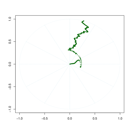
(b)

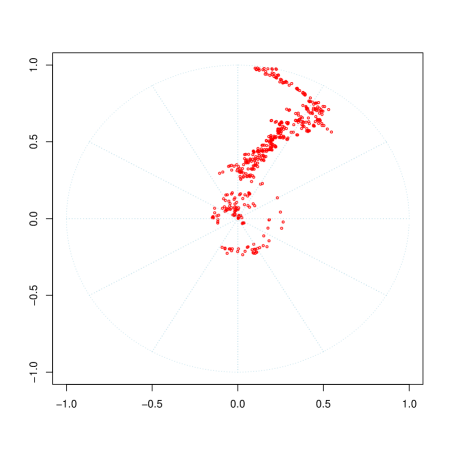
(c)

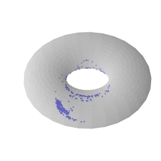
(d)

Figure 1. (A) scatter plot of the wind-wave directions on the flat torus. (B) circular temporal plot of the direction of the wave. (C) circular temporal plot of the wind direction, and (D) scatter plot of the wind-wave directions on the curved torus.

(a)

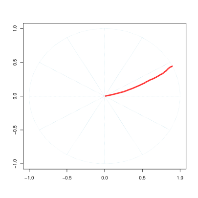
(b)

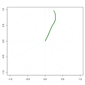
(c)

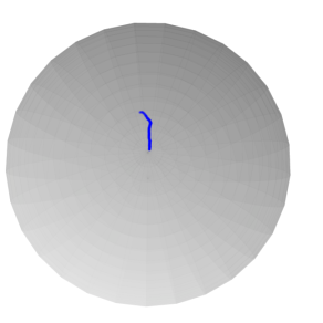
(d)

Figure 2. (A) scatter plot of the latitude-longitude directions on the flat sphere. (B) circular temporal plot of the latitude. (C) circular temporal plot of the longitude, and (D) scatter plot of the latitude-longitude directions on the sphere.

2. Intrinsic Geometry of smooth surfaces

Before getting into the proposed method, we briefly discuss some basic tools from Riemannian geometry. Here, we introduce a few definitions of tangent space, the first fundamental form, and the area element. The reader may see Gallier and Quaintance (2020) for details.

Definition 1.

Let $\mathcal{M}$ be a Riemannian surface. Then the set of all tangent vectors $v$ at $x\in\mathcal{M}$ is called the tangent space to the point $x$ and it is denoted by $T_{x}\mathcal{M}.$

Let $\mathcal{M}\subset\mathbb{R}^{3}$ be a Riemannian surface defined by $X:\mathbb{R}^{2}\rightarrow\mathcal{M}.$ Then a curve $\gamma(t)$ on $\mathcal{M}$ parametrized by $t\in[a,b]$ can be defined as $\gamma(t)=X(u(t),v(t)).$ Therefore, the velocity vector can be obtained as

$$\gamma^{\prime}(t)=\dfrac{\partial X}{\partial u}\dfrac{du}{dt}+\dfrac{\partial X}{\partial v}\dfrac{dv}{dt}=[X_{u},X_{v}][u^{\prime},v^{\prime}]^{T}$$

Thus, we can represent the velocity vector as the linear combination of the basis vectors $X_{u}=\dfrac{\partial X}{\partial u}$ and $X_{v}=\dfrac{\partial X}{\partial v}$, with coefficients $u^{\prime}=\dfrac{du}{dt}$ and $v^{\prime}=\dfrac{dv}{dt}.$ Let $s(t)$ be the arc length along $\gamma$ with $s(a)=0$ then $s(t)=\int_{a}^{t}||\gamma^{\prime}(r)||\,dr,$ so, we have $\dfrac{ds}{dt}=||\gamma^{\prime}(t)||.$ Now, the first fundamental form or metric form of the surface $\mathcal{M}$ can be obtained as

$$\left(\dfrac{ds}{dt}\right)^{2} = \langle\gamma^{\prime}(t),\gamma^{\prime}(t)\rangle$$

$$= \langle(u^{\prime}X_{u}+v^{\prime}X_{v}),(u^{\prime}X_{u}+v^{\prime}X_{v})\rangle$$

$$= (u^{\prime})^{2}\langle X_{u},X_{u}\rangle+2u^{\prime}v^{\prime}\langle X_{u},X_{v}\rangle+(v^{\prime})^{2}\langle X_{v},X_{v}\rangle$$

$$\equiv (u^{\prime})^{2}~{}E+2u^{\prime}v^{\prime}~{}F+(v^{\prime})^{2}~{}G$$

$$= \begin{bmatrix}u^{\prime}\\ v^{\prime}\end{bmatrix}^{T}\begin{bmatrix}E&F\\ F&G\end{bmatrix}\begin{bmatrix}u^{\prime}\\ v^{\prime}\end{bmatrix}$$

where $E=\langle X_{u},X_{u}\rangle,$ $F=\langle X_{u},X_{v}\rangle$, and $G=\langle X_{v},X_{v}\rangle,$ with usual inner-product $\langle\cdot,\cdot\rangle$.

Definition 2.

The area element, $dA$ of the surface $\mathcal{M}$ determined by $X(u,v)$ is defined by

$$dA=|X_{u}\times X_{v}|~{}dudv=\sqrt{EG-F^{2}}~{}dudv.$$

Hence, the total surface area of the surface $\mathcal{M}$ is

$$A=\int\int dA~{}dudv=\int\int\sqrt{EG-F^{2}}~{}dudv.$$

2.1. Intrinsic geometry of torus

The rest of our work will be based on the curved torus defined by the parametric equation

$$X(\phi,\theta)=\{(R+r\cos{\theta})\cos{\phi},(R+r\cos{\theta})\sin{\phi},r\sin{\theta}\}\subset\mathbb{R}^{3},$$ (1)

with the parameter space $\{(\phi,\theta):0<\phi,\theta<2\pi\}=\mathbb{S}_{1}\times\mathbb{S}_{1},$ known as 2-torus. Now, the partial derivatives of $X$ with respect to $\phi$, and $\theta$ are

$$X_{\phi}=\{-(R+r\cos{\theta})\sin{\phi},(R+r\cos{\theta})\cos{\phi},0\}$$

and

$$X_{\theta}=\{-r\sin{\theta}\cos{\phi},-r\sin{\theta}\sin{\phi},r\cos{\theta}\}$$

respectively. Hence, the coefficients of the first fundamental form are

$$E=\langle X_{\phi},X_{\phi}\rangle =(R+r\cos{\theta})^{2}$$ (2)

$$F=\langle X_{\phi},X_{\theta}\rangle =0$$

$$G=\langle X_{\theta},X_{\theta}\rangle =r^{2}$$

leading to the area element of the curved torus (Equation-1)

$$dA^{(\mathcal{T})}=r(R+r\cos{\theta})~{}d\theta~{}d\phi$$ (3)

from the Definition-2. We will use this idea to introduce the notion of variance for angular random variables.

2.1.1. Area Decomposition of Curved Torus

Let $\phi,\theta\in[0,2\pi)$ denote a torus’s horizontal and vertical angles, respectively. We begin by defining the area between two points on the surface of the torus. Let $(\phi_{1},\theta_{1})$ and $(\phi_{2},\theta_{2})$ be two points on the flat torus $[0,2\pi)\times[0,2\pi)$, then the proportionate area included between these two diagonally opposite points when mapped on the surface of the torus with horizontal and vertical radius $R$ and $r$, respectively can be computed by the following method using Equation-3 considering $0<\phi_{1}<\phi_{2}<2\pi$ and $0<\theta_{1}<\theta_{2}<2\pi.$ Note that for two such diagonally opposite points $(\phi_{1},\theta_{1})$ and $(\phi_{2},\theta_{2})$ on flat torus, the surface on the torus get partitioned into four mutually exclusive and exhaustive subsets as images (using Equation-1) of the following sets $\mathbb{T}_{1}:=[\phi_{1},\phi_{2}]\times[\theta_{1},\theta_{2}]$, $\mathbb{T}_{2}:=([\phi_{2},2\pi]\cup[0,\phi_{1}])\times[\theta_{1},\theta_{2}]$, $\mathbb{T}_{3}:=[\phi_{1},\phi_{2}]\times([\theta_{2},2\pi]\cup[0,\theta_{1}])$ and $\mathbb{T}_{4}:=([\phi_{2},2\pi]\cup[0,\phi_{1}])\times([\theta_{2},2\pi]\cup[0,\theta_{1}]).$ Let us call these regions $\mathbb{R}_{1}$, $\mathbb{R}_{2}$, $\mathbb{R}_{3}$ and $\mathbb{R}_{4}$ with the corresponding areas $A^{\mathcal{T}}_{1}$, $A^{\mathcal{T}}_{2}$, $A^{\mathcal{T}}_{3}$ and $A^{\mathcal{T}}_{4}$ respectively. A diagrammatic representation of this decomposition is given in Figure-3. We now provide details of the computation of the areas $A^{\mathcal{T}}_{1}$, $A^{\mathcal{T}}_{2}$, $A^{\mathcal{T}}_{3}$ and $A^{\mathcal{T}}_{4}$.

• Case-1: Using Equation-3 on ${\mathbb{T}_{1}}$ we get

  $$A^{\mathcal{T}}_{1} =\displaystyle\iint_{\mathbb{T}_{1}}dA^{(\mathcal{T})}=\int_{\phi_{1}}^{\phi_{2}}\int_{\theta_{1}}^{\theta_{2}}dA^{(\mathcal{T})}=rR\int_{\phi_{1}}^{\phi_{2}}d\phi~{}\int_{\theta_{1}}^{\theta_{2}}(1+\frac{r}{R}\cos{\theta})~{}d\theta.$$

  $$=rR(\phi_{2}-\phi_{1})\left[(\theta_{2}-\theta_{1})+\frac{r}{R}\left(\sin{\theta_{2}}-\sin{\theta_{1}}\right)\right].$$ (4)

• Case-2: Using Equation-3 on ${\mathbb{T}_{2}}$ we get

  $$A^{\mathcal{T}}_{2} =\displaystyle\iint_{\mathbb{T}_{2}}dA^{(\mathcal{T})}=\int_{\phi_{2}}^{2\pi}\int_{\theta_{1}}^{\theta_{2}}dA^{(\mathcal{T})}+\int_{0}^{\phi_{1}}\int_{\theta_{1}}^{\theta_{2}}dA^{(\mathcal{T})}$$

  $$=rR[2\pi-(\phi_{2}-\phi_{1})]\left[(\theta_{2}-\theta_{1})+\frac{r}{R}\left(\sin{\theta_{2}}-\sin{\theta_{1}}\right)\right]$$ (5)

• Case-3: Using Equation-3 on ${\mathbb{T}_{3}}$ we get

  $$A^{\mathcal{T}}_{3} =\displaystyle\iint_{\mathbb{T}_{3}}dA^{(\mathcal{T})}=\int_{\phi_{1}}^{\phi_{2}}\int_{\theta_{2}}^{2\pi}dA^{(\mathcal{T})}+\int_{\phi_{1}}^{\phi_{2}}\int_{0}^{\theta_{1}}dA^{(\mathcal{T})}$$

  $$=rR(\phi_{2}-\phi_{1})\left[(2\pi-(\theta_{1}-\theta_{2})+\frac{r}{R}(\sin{\theta_{1}}-\sin{\theta_{2}})\right]$$ (6)

• Case-4: Using Equation-3 on ${\mathbb{T}_{4}}$ we get

  $$A^{\mathcal{T}}_{4} =\displaystyle\iint_{\mathbb{T}_{4}}dA^{(\mathcal{T})}=\int_{\phi_{2}}^{2\pi}\int_{\theta_{2}}^{2\pi}dA^{(\mathcal{T})}+\int_{\phi_{2}}^{2\pi}\int_{0}^{\theta_{1}}dA^{(\mathcal{T})}+\int_{0}^{\phi_{1}}\int_{\theta_{2}}^{2\pi}dA^{(\mathcal{T})}+\int_{0}^{\phi_{1}}\int_{0}^{\theta_{1}}dA^{(\mathcal{T})}$$

  $$=rR\left[2\pi-(\phi_{2}-\phi_{1})\right]\left[(2\pi-(\theta_{1}-\theta_{2})+\frac{r}{R}(\sin{\theta_{1}}-\sin{\theta_{2}})\right].$$ (7)

Analogous to the notion of circular distance - which is the length of the smaller arc between two angles, and the notion of geodesic distance on a surface - which is the length of the shortest path joining two points on the surface, we define the proportionate area included between these two diagonally opposite points $(\phi_{1},\theta_{1})$, $(\phi_{2},\theta_{2})$ as given below. It may be noted that, since $r$ and $R$ are arbitrary and $\min\{A^{\mathcal{T}}_{1},A^{\mathcal{T}}_{2},A^{\mathcal{T}}_{3},A^{\mathcal{T}}_{4}\}$ is dependent on $rR$, we divide it by $4\pi^{2}rR$ which is the total area of the torus to remove this dependency.

Definition 3.

The proportionate area included between these two diagonally opposite points $(\phi_{1},\theta_{1})$, $(\phi_{2},\theta_{2})$ is defined as

$$A_{T}\left[(\phi_{1},\theta_{1}),(\phi_{2},\theta_{2})\right]=\frac{\min\{A^{\mathcal{T}}_{1},A^{\mathcal{T}}_{2},A^{\mathcal{T}}_{3},A^{\mathcal{T}}_{4}\}}{4\pi^{2}rR}.$$

2.2. Intrinsic geometry of sphere

The rest of our work will be based on the sphere defined by the parametric equation

$$X(\phi,\theta)=\{r\sin{\theta}\cos{\phi},r\sin{\theta}\sin{\phi},r\cos{\theta}\}\subset\mathbb{R}^{3},$$ (8)

with the parameter space $\{(\phi,\theta):0\leq\phi<2\pi,~{}~{}0\leq\theta<\pi\}$. Now, the partial derivatives of $X$ with respect to $\phi$, and $\theta$ are

$$X_{\phi}=\{-r\sin{\theta}\sin{\phi},r\sin{\theta}\cos{\phi},0\}$$

and

$$X_{\theta}=\{r\cos{\theta}\cos{\phi},r\cos{\theta}\sin{\phi},-r\sin{\theta}\}$$

respectively. Hence, the coefficients of the first fundamental form are

$$E=\langle X_{\phi},X_{\phi}\rangle =r^{2}\sin^{2}{\theta}$$ (9)

$$F=\langle X_{\phi},X_{\theta}\rangle =0$$

$$G=\langle X_{\theta},X_{\theta}\rangle =r^{2}$$

leading to the area element of the curved torus (Equation-8)

$$dA^{(\mathcal{S})}=r^{2}\sin{\theta}~{}d\theta~{}d\phi$$ (10)

from the Definition-2. We will use this idea to introduce the notion of variance for angular random variables.

2.2.1. Area Decomposition of Sphere

Let $\phi\in[0,2\pi)$, $\theta\in[0,\pi)$ denote the horizontal and vertical angles of a sphere, respectively. We begin by defining the area between two points on the surface of the sphere. Let $(\phi_{1},\theta_{1})$ and $(\phi_{2},\theta_{2})$ be two points on the sphere $[0,2\pi)\times[0,\pi)$, then the proportionate area included between these two diagonally opposite points when mapped on the surface of the sphere with radius $r$ can be computed by the following method using Equation-10 considering $0<\phi_{1}<\phi_{2}<2\pi$ and $0<\theta_{1}<\theta_{2}<\pi.$ Note that for two such diagonally opposite points $(\phi_{1},\theta_{1})$ and $(\phi_{2},\theta_{2})$ on flat sphere, the surface on the sphere get partitioned into four mutually exclusive and exhaustive subsets as images (using Equation-8) of the following sets $\mathbb{S}_{1}:=[\phi_{1},\phi_{2}]\times[\theta_{1},\theta_{2}]$, $\mathbb{S}_{2}:=([\phi_{2},2\pi]\cup[0,\phi_{1}])\times[\theta_{1},\theta_{2}]$, $\mathbb{S}_{3}:=[\phi_{1},\phi_{2}]\times([\theta_{2},\pi]\cup[0,\theta_{1}])$ and $\mathbb{S}_{4}:=([\phi_{2},2\pi]\cup[0,\phi_{1}])\times([\theta_{2},\pi]\cup[0,\theta_{1}]).$ Let us call these areas $A^{\mathcal{S}}_{1}$, $A^{\mathcal{S}}_{2}$, $A^{\mathcal{S}}_{3}$ and $A^{\mathcal{S}}_{4}$ respectively. A diagrammatic representation of this decomposition is given in Figure-3. We now provide details of the computation of the areas $A^{\mathcal{S}}_{1}$, $A^{\mathcal{S}}_{2}$, $A^{\mathcal{S}}_{3}$ and $A^{\mathcal{S}}_{4}$.

• Case-1: Using Equation-3 on ${\mathbb{S}_{1}}$ we get

  $$A^{\mathcal{S}}_{1} =\displaystyle\iint_{\mathbb{S}_{1}}dA^{(\mathcal{S})}=\int_{\phi_{1}}^{\phi_{2}}\int_{\theta_{1}}^{\theta_{2}}dA^{(\mathcal{S})}=r\int_{\phi_{1}}^{\phi_{2}}d\phi~{}\int_{\theta_{1}}^{\theta_{2}}\sin{\theta}~{}d\theta.$$

  $$=r^{2}(\phi_{2}-\phi_{1})\left(\cos{\theta_{1}}-\cos{\theta_{2}}\right).$$ (11)

• Case-2: Using Equation-3 on ${\mathbb{S}_{2}}$ we get

  $$A^{\mathcal{S}}_{2} =\displaystyle\iint_{\mathbb{S}_{2}}dA^{(\mathcal{S})}=\int_{\phi_{2}}^{2\pi}\int_{\theta_{1}}^{\theta_{2}}dA^{(\mathcal{S})}+\int_{0}^{\phi_{1}}\int_{\theta_{1}}^{\theta_{2}}dA^{(\mathcal{S})}$$

  $$=r^{2}[2\pi-(\phi_{2}-\phi_{1})]\left(\cos{\theta_{1}}-\cos{\theta_{2}}\right)$$ (12)

• Case-3: Using Equation-3 on ${\mathbb{S}_{3}}$ we get

  $$A^{\mathcal{S}}_{3} =\displaystyle\iint_{\mathbb{S}_{3}}dA^{(\mathcal{S})}=\int_{\phi_{1}}^{\phi_{2}}\int_{\theta_{2}}^{\pi}dA^{(\mathcal{S})}+\int_{\phi_{1}}^{\phi_{2}}\int_{0}^{\theta_{1}}dA^{(\mathcal{S})}$$

  $$=r^{2}(\phi_{2}-\phi_{1})\left[2+(\cos{\theta_{2}}-\cos{\theta_{1}})\right]$$ (13)

• Case-4: Using Equation-3 on ${\mathbb{S}_{4}}$ we get

  $$A^{\mathcal{S}}_{4} =\displaystyle\iint_{\mathbb{S}_{4}}dA^{(\mathcal{S})}=\int_{\phi_{2}}^{2\pi}\int_{\theta_{2}}^{\pi}dA^{(\mathcal{S})}+\int_{\phi_{2}}^{2\pi}\int_{0}^{\theta_{1}}dA^{(\mathcal{S})}+\int_{0}^{\phi_{1}}\int_{\theta_{2}}^{\pi}dA^{(\mathcal{S})}+\int_{0}^{\phi_{1}}\int_{0}^{\theta_{1}}dA^{(\mathcal{S})}$$

  $$=r^{2}\left[2\pi-(\phi_{2}-\phi_{1})\right]\left[2+(\cos{\theta_{2}}-\cos{\theta_{1}})\right].$$ (14)

Now, below, we define the proportionate area included between these two diagonally opposite points $(\phi_{1},\theta_{1})$, $(\phi_{2},\theta_{2})$ as given below. It may be noted that, since $r$ is arbitrary and $\min\{A^{\mathcal{S}}_{1},A^{\mathcal{S}}_{2},A^{\mathcal{S}}_{3},A^{\mathcal{S}}_{4}\}$ is dependent on $r$, we divide it by total surface area of the sphere, $4\pi r^{2}$ which is the total area of the torus to remove this dependency.

Definition 4.

The proportionate area included between these two diagonally opposite points $(\phi_{1},\theta_{1})$, $(\phi_{2},\theta_{2})$ is defined as

$$A_{S}\left[(\phi_{1},\theta_{1}),(\phi_{2},\theta_{2})\right]=\frac{\min\{A^{\mathcal{S}}_{1},A^{\mathcal{S}}_{2},A^{\mathcal{S}}_{3},A^{\mathcal{S}}_{4}\}}{4\pi r^{2}}.$$

3. Curved dispersion matrix

In this section, we define “curved variance” and “curved co-variance” for the toroidal and spherical data as follows. Following the Definition-3 and 4, we obtain the proportionate area between $(0,0)$ to any arbitrary point $(\phi,\theta)$ on the curved torus or sphere, respectively, as:

$$A^{(0)}(\phi,\theta)=\displaystyle\begin{cases}A_{T}\left[(0,0),(\phi,\theta)\right]&\text{for the curved torus.}\\ A_{S}\left[(0,0),(\phi,\theta)\right]&\text{for the sphere.}\end{cases}$$ (15)

Now, we apply this notion to angular data for defining the square of an angle as well as the variance of an angular random variable as follows.

Definition 5.

The square of an angle $\theta$ is defined as

$$A_{C}^{(0)}(\theta)=A^{(0)}(\theta,\theta)=\displaystyle\begin{cases}A_{T}\left[(0,0),(\theta,\theta)\right]&\text{for the curved torus}\mbox{~{}with~{}}\frac{r}{R}=1.\\ A_{S}\left[(0,0),(\theta,\theta)\right]&\text{for the sphere.}\end{cases}$$ (16)

Definition 6.

Let $\Theta$ be a zero-centered circular random variable with probability density function $f(\theta)$ on the unit circle $\mathbb{S}_{1}$. Then, the curved-variance of the random variable $\Theta$ is

$$CVar(\Theta)=E_{f}\left[A_{C}^{(0)}(\Theta)\right].$$

If the circular mean of $\Theta\mbox{~{}is~{}}\mu\neq 0$ then $\Theta$ can be replaced by $\Theta^{\prime}=\left[(\Theta-\mu)\mod k\pi\right]$, where $k=2$ when $\Theta\in[0,2\pi)$, and $k=1$ when $\Theta\in[0,\pi).$

If a random sample $\theta_{1},\ldots,\theta_{n}$ is given then using weak law of large number (WLLN), $CVar(\Theta)$ can be consistently estimated as $\widehat{CVar(\Theta)}=\displaystyle\frac{1}{n}\sum_{i=1}^{n}A_{C}^{(0)}\left[(\theta_{i}-{\mu})\mod k\pi\right],$ when $\mu$ is known. When $\mu$ is unknown we can use the plug-in estimator

$$\widetilde{CVar(\Theta)}=\displaystyle\frac{1}{n}\sum_{i=1}^{n}A_{C}^{(0)}\left[(\theta_{i}-\hat{\mu})\mod k\pi\right],$$

where $\hat{\mu}$ is the estimated circular mean of the data. Continuing the analogy we define the curved co-variance in the following section.

3.1. Curved co-variance

In this section, we will define a measure similar to covariance in linear data for angular random variables, termed “area covariance” (ACov), using Equation 15.

Definition 7.

Let $\Theta$, $\Phi$ be two zero-centered circular random variables with the joint probability density function $f(\phi,\theta)$. Then, using Equation-15, the “area covariance” is defined as:

$$ACov(\Phi,\Theta)=\displaystyle E_{f(\phi,\theta)}\left[\sqrt{A^{(0)}_{C}(\phi)\cdot A^{(0)}_{C}(\theta)}\right].$$

If a random sample $\{(\phi_{1},\theta_{1}),\ldots,(\phi_{n},\theta_{n})\}$ is given then using WLLN, $ACov(\Phi,\Theta)$ can be consistently estimated as

$$\widehat{ACov(\Phi,\Theta)}=\displaystyle\frac{1}{n}\sum_{i=1}^{n}\sqrt{\left[A^{(0)}_{C}\left((\phi_{i}-{\mu_{\phi}})\mod 2\pi\right)\right]\left[A^{(0)}_{C}\left((\theta_{i}-{\mu_{\theta}})\mod k\pi\right)\right]},$$

when $\mu_{\phi},\mu_{\theta}$ are known mean directions. When $\mu_{\phi},\mu_{\theta}$ are unknown, we can use the plug-in estimator

$$\widetilde{ACov(\Phi,\Theta)}=\displaystyle\frac{1}{n}\sum_{i=1}^{n}\sqrt{\left[A^{(0)}_{C}\left((\phi_{i}-{\hat{\mu}_{\phi}})\mod 2\pi\right)\right]\left[A^{(0)}_{C}\left((\theta_{i}-{\hat{\mu}_{\theta}})\mod k\pi\right)\right]},$$

where $\hat{\mu}_{\phi},\hat{\mu}_{\theta}$ are the estimated circular mean directions of the data. $k$ can be suitably chosen based on the range of the angular data as introduced in Definition-6. Without loss of generality assuming a marginal probability density function be denoted as $f(\cdot)$, we obtain from Definition-7 and Equation-16

$$ACov(\cdot,\cdot)=\displaystyle E_{f(\cdot)}\left[A^{(0)}(\cdot,\cdot)\right]=E_{f(\cdot)}\left[A_{C}^{(0)}(\cdot)\right]=CVar(\cdot).$$ (17)

for any of the angular random variables $\Phi$ and $\Theta.$ Here, we can find $f(\theta)$ from the joint probability distribution function $f(\phi,\theta)$ as $f(\theta)=\displaystyle\int_{\phi=0}^{2\pi}f(\phi,\theta)~{}d\phi$. Using the expression of $f(\theta)$ in the Equation-17 we have

$$CVar(\Theta)=E_{f(\phi,\theta)}\left[A^{(0)}(\theta,\theta)\right].$$ (18)

Similarly, we can say that

$$CVar(\Phi)=E_{f(\phi,\theta)}\left[A^{(0)}(\phi,\phi)\right].$$ (19)

Lemma 1.

Let, $a_{11}=CVar(\Phi),a_{22}=CVar(\Theta)$, and $a_{12}=a_{21}=ACov(\Phi,\Theta)$, then the curve dispersion (CD) matrix $\Sigma_{A}$ defined by

$$\Sigma_{A}=\begin{pmatrix}a_{11}&a_{12}\\ a_{21}&a_{22}\end{pmatrix}$$

is a symmetric and positive semi-definite matrix.

Proof.

By construction, the matrix, $\Sigma_{A}$ is symmetric. Now consider

$$a_{11}\cdot a_{22} =E_{f(\phi,\theta)}\left[A^{(0)}(\phi,\phi)\right]\cdot E_{f(\phi,\theta)}\left[A^{(0)}(\theta,\theta)\right]$$

$$=E_{f(\phi,\theta)}\left[\left(\sqrt{A^{(0)}(\phi,\phi)}\right)^{2}\right]\cdot E_{f(\phi,\theta)}\left[\left(\sqrt{A^{(0)}(\theta,\theta)}\right)^{2}\right]$$

$$\geq\left(E_{f(\phi,\theta)}\left[\sqrt{A^{(0)}(\phi,\phi)\cdot A^{(0)}(\theta,\theta)}\right]\right)^{2}$$

$$a_{11}\cdot a_{22} \geq a_{12}^{2}\mbox{ by Cauchy\textendash Schwarz inequality}$$ (20)

This implies that $|\Sigma_{A}|\geq 0$ and $trace(\Sigma_{A})>0$. Hence, the eigenvalues of $\Sigma_{A}$ are non-negative. As a consequence $\Sigma_{A}$ is positive semi-definite. ∎

Remark 1.

The proportionate area $A_{T}\left[(\phi_{1},\theta_{1})(\phi_{2},\theta_{2})\right]\in[0,\frac{1}{4}]$. It may be noted that $A_{T}\left[(\phi_{1},\theta_{1})(\phi_{2},\theta_{2})\right]$ only depends only on $\frac{r}{R}$ where, $0<\frac{r}{R}\leq 1$.

Remark 2.

$CVar$ does not depend on the (known) mean direction.

Remark 3.

As a natural choice, put $(\phi,\theta)=(0,0)$ in Equation-1, the zero-point on the curved torus is assumed to be $(R+r,0,0)$, and counter-clock-wise rotation is considered to be conventional.

Remark 4.

For univariate linear random variable $X$ with expectation $\eta$ it is well-known that

$$Var(X)=E(X-\eta)^{2}=EX^{2}-\eta^{2}.$$

Though Definition-6 is a generalization of the definition $Var(X)=E(X-\eta)^{2}$, but the simplification $Var(X)=EX^{2}-\eta^{2}$ is not generalizable to the case of angular data. i.e. $E_{f}(A_{C}^{(0)}([(\Theta-\mu)\mod 2\pi]))\neq E_{f}(A_{C}^{(0)}(\Theta))-A_{C}^{(0)}(\mu)$ in general, where $\Theta$ is a circular random variable with circular mean $\mu$. Consider a circular random variable $\Theta$ with probability density function $f(\theta)$ and mean direction at $\pi$ as a counter-example. Note that

$$A_{C}^{(0)}(\theta)-A_{C}^{(0)}(\pi)=A_{C}^{(0)}(\theta)-\frac{1}{4}\leq 0\mbox{~{}~{}for all }\theta\in[0,2\pi).$$

As a consequence $\displaystyle E_{f}\left[A_{C}^{(0)}(\Theta)\right]-\frac{1}{4}\leq 0$. Hence, $\displaystyle E_{f}\left[A_{C}^{(0)}(\Theta)\right]-\frac{1}{4}<0$ unless $\Theta$ is degenerate at $\pi$. Thus we see that $CVar(\Theta)=E_{f}(A_{C}^{(0)}([(\Theta-\pi)\mod 2\pi]))\neq E_{f}(A_{C}^{(0)}(\Theta))-A_{C}^{(0)}(\pi)$ when $\Theta$ is not degenerate at $\pi$. The definition of ${CVar}$ considers the non-constant curvature through the area element of the surface of the torus. A similar approach, when applied to linear univariate data, would yield the usual definition of variance of linear univariate data since the curvature is constant.

Remark 5.

When we consider the curved torus with the radii $r,$ and $R$ for vertical and horizontal circles, respectively, the distribution $f(\phi,\theta)$ is a toroidal distribution, and hence the curved variance (using $r=R=1$) and curved co-variance will be calculated using specifications of the radius of the curved torus.

Remark 6.

When we consider the sphere with the radius, $r$, the distribution $f(\phi,\theta)$ is a spherical distribution, and hence the curved variance and curved co-variance will be calculated using the formulas defined for the sphere.

4. Detection of mean change in the trorodal data

Let $\Psi_{i}=(\phi_{i},\theta_{i})\in[0,2\pi)\times[0,2\pi),\mbox{~{}~{}for~{}~{}}i=1,\ldots,n$ be independent angular random vectors. We are interested in addressing the following testing problem :

$$H_{0t} : \Psi_{i}\overset{\mathrm{i.i.d.}}{\scalebox{1.5}{$\sim$}}F(\psi;\bm{\xi}_{1},\bm{\eta})\mbox{~{}~{}for all~{}~{}}i=1,2,\ldots n,$$

$$H_{1t} : \begin{cases}\Psi_{i}\overset{\mathrm{i.i.d.}}{\scalebox{1.5}{$\sim$}}F(\psi;\bm{\xi}_{1},\bm{\eta})&\text{, }1\leq i\leq k^{*}\\ \Psi_{i}\overset{\mathrm{i.i.d.}}{\scalebox{1.5}{$\sim$}}F(\theta;\bm{\xi}_{2},\bm{\eta})&\text{, }(k^{*}+1)\leq i\leq n,\end{cases}$$ (21)

where $\bm{\xi}_{1},\bm{\xi}_{2}$ are suitable vector-valued parameters representing the location (mean directions) of the distributions and $\bm{\xi}_{1}\neq\bm{\xi}_{2},$ under the alternative hypothesis $H_{1t}$. In both hypotheses, it is assumed that the concentration-parameter vector $\bm{\eta}$ remains unchanged for the entire sequence. Here we assume that $\bm{\eta}$ is unrelated to $\bm{\xi}_{1}$ and $\bm{\xi}_{2}$. We consider the corresponding mean shifted angles for

$$\phi_{i}^{c}=[(\phi_{i}-\hat{\mu}_{\phi})\mod 2\pi]\mbox{~{}and~{}}\theta_{i}^{c}=[(\theta_{i}-\hat{\mu}_{\theta})\mod 2\pi],$$

where $\hat{\mu}_{\phi}$, $\hat{\mu}_{\theta}$ are the estimated circular mean direction of $\phi_{i},\theta_{i},$ respectively, $\text{~{}for~{}}i=1,\cdots,n$, on the surface of a curved torus. Now onwards $\hat{\mu}_{\phi}$, $\hat{\mu}_{\theta}$ are treated to be constants. This is reasonable particularly when the sample size is large. Without loss of generality, the sign of the circular random variables, $\phi,\theta\in[0,2\pi)$ can be defined as

$$sgn(\phi) = 2\left(\delta_{(\phi<\pi)}-0.5\right)\in\{-1,1\}.$$ (22)

Similarly, it will hold for $\theta$ as well.

Using the Equation-16 (for torus), we get the corresponding square areas as

$$\hat{a}_{i}=sgn^{2}(\phi_{i}^{c})A_{C}^{(0)}(\phi_{i}^{c})\mbox{~{}~{}and~{}~{}}\hat{b}_{i}=sgn^{2}(\theta_{i}^{c})A_{C}^{(0)}(\theta_{i}^{c}),$$

respectively, together with $\widehat{(ab)}_{i}=sgn(\phi_{i}^{c})~{}~{}sgn(\theta_{i}^{c})\sqrt{A_{C}^{(0)}(\phi_{i}^{c})\cdot A_{C}^{(0)}(\theta_{i}^{c})}$. Hence, calculate the curved variance and curved co-variance as

$$cv_{\phi} = \frac{1}{n}\sum_{i=1}^{n}~{}\hat{a}_{i},\hskip 11.38092ptcv_{\theta}=\frac{1}{n}\sum_{i=1}^{n}~{}\hat{b}_{i},~{}\mbox{and~{}}ccv_{\phi\theta}=\frac{1}{n}\sum_{i=1}^{n}~{}\widehat{(ab)}_{i}.$$ (23)

Now, we obtain the curved dispersion matrix and its inverse as

$$\Sigma_{(t)}=\begin{bmatrix}cv_{\phi}&ccv_{\phi\theta}\\ ccv_{\phi\theta}&cv_{\theta}\end{bmatrix}$$ (24)

$$\Sigma_{(t)}^{-1}=\frac{1}{cv_{\phi}\cdot cv_{\theta}-ccv_{\phi\theta}^{2}}\begin{bmatrix}cv_{\theta}&-ccv_{\phi\theta}\\ -ccv_{\phi\theta}&cv_{\phi}\end{bmatrix}\equiv\begin{bmatrix}\iota cv_{\phi}&\iota ccv_{\phi\theta}\\ \iota ccv_{\phi\theta}&\iota cv_{\theta}\end{bmatrix}.$$ (25)

We consider the corresponding mean $(\mu_{\phi},\mu_{\theta})$ of the initial $\lambda$% data under the assumption that the changepoint may occur in the rest $(100-\lambda)\%$ of the data. Hence we obtain

$$\phi_{i}^{m}=[(\phi_{i}-\mu_{\phi})\mod 2\pi]\mbox{~{}and~{}}\theta_{i}^{m}=[(\theta_{i}-\mu_{\theta})\mod 2\pi],$$

where $\mu_{\phi}$, $\mu_{\theta}$ are the circular mean direction before changepoint of $\phi_{i},\theta_{i},$ respectively, $\text{~{}for~{}}i=1,\cdots,n$, on the surface of a curved torus.

Consider $\tilde{a}_{i}=sgn^{2}(\phi^{m}_{i})A_{C}^{(0)}(\phi^{m}_{i})$, and $\tilde{b}_{i}=sgn^{2}(\theta^{m}_{i})A_{C}^{(0)}(\theta^{m}_{i})$, respectively, together with $\widetilde{(ab)}_{i}=sgn(\phi^{m}_{i})~{}~{}sgn(\theta^{m}_{i})\sqrt{A_{C}^{(0)}(\phi^{m}_{i})\cdot A_{C}^{(0)}(\theta^{m}_{i})}$. We calculate an expression analogous to the quadratic form associated with the Mahalanobis distance using the matrix $\Sigma_{(t)}^{-1}$ and the vector $\left(sgn(\phi^{m}_{i})\sqrt{A_{C}^{(0)}(\phi^{m}_{i})},sgn(\theta^{m}_{i})\sqrt{A_{C}^{(0)}(\theta^{m}_{i})}\right)^{T}$ to obtain

$$Q_{i} = \iota cv_{\phi}\cdot\tilde{a}_{i}+\iota cv_{\theta}\cdot\tilde{b}_{i}+2\cdot\iota ccv_{\phi\theta}\cdot\widetilde{(ab)}_{i}$$ (26)

$\mbox{~{}for~{}}i=1,2,\ldots n$. Now, consider the estimated variance of the sequence, $\{Q\}$ as

$$S_{Q}^{2}{=}\frac{1}{n-1}\sum_{i=1}^{n}\left(Q_{i}-\bar{Q}\right)^{2},$$

where $n~{}\bar{Q}=\displaystyle\sum_{i=1}^{n}Q_{i},$ and we define a CUSUM process

$$U(k)=\frac{1}{\sqrt{n~{}S_{Q}^{2}}}\left[\sum_{i=1}^{k}Q_{i}-k\bar{Q}\right]\mbox{~{}~{}for all~{}~{}}k=1,\ldots,n$$ (27)

to obtain the test statistic

$$\mathcal{M}_{n}=\displaystyle\max_{1\leq k<n}|U(k)|.$$ (28)

Hence, we reject the null hypothesis, $H_{0t}$, if $\mathcal{M}_{n}>k_{\alpha}$, where, $k_{\alpha}$ is the upper $\alpha$ point of the exact (or asymptotic) distribution of $\mathcal{M}_{n}$ under the null hypothesis. The closed-form distribution of $\mathcal{M}_{n}$ is not available; hence, we need to take recourse to simulation to obtain the cut-off value $k_{\alpha}$. When $n$ is large, the limiting distribution of $\mathcal{M}_{n}$ can be derived as follows. Let us consider $u\in(0,1)$, and denote $k=\lfloor{nu}\rfloor$. Hence, from Equation-27 we can write

$$T_{n}(u)=T(\lfloor{nu}\rfloor)=\left|\frac{1}{\sqrt{n~{}S_{Q}^{2}}}\left[\sum_{i=1}^{\lfloor{nu}\rfloor}Q_{i}-u\sum_{i=1}^{n}Q_{i}\right]\right|.$$ (29)

Then, with the proper embedding of Skorohod topology in $D[0,1]$ (see Billingsley, 2013, Ch. 3), under the null hypothesis, $H_{0t}$, and as $n\uparrow\infty$, the process $T_{n}(u)$ converges weakly to $|B_{0}(u)|,$ where $B_{0}(u)$ is the standard Brownian bridge on $[0,1].$ As a consequence

$$\mathcal{M}_{n}\overset{d}{\to}\displaystyle\sup_{0<u<1}|B_{0}(u)|=K_{\infty},\mbox{~{}~{}say}.$$ (30)

Now, we can compute the upper-$\alpha$ value, $k_{\alpha},$ from the above limiting random variable $K_{\infty}$ which follows the Kolmogorov distribution of the test statistic (Equation-30) with large sample approximation discussed in Section 6.

5. Detection of mean change in spherical data

Let $\Psi_{i}=(\phi_{i},\theta_{i})\in[0,2\pi)\times[0,\pi),\mbox{~{}~{}for~{}~{}}i=1,\ldots,n$ be independent angular random vectors. We are interested in addressing the following testing problem :

$$H_{0s} : \Psi_{i}\overset{\mathrm{i.i.d.}}{\scalebox{1.5}{$\sim$}}F(\psi;\bm{\xi}_{1},\bm{\eta})\mbox{~{}~{}for all~{}~{}}i=1,2,\ldots n,$$

$$H_{1s} : \begin{cases}\Psi_{i}\overset{\mathrm{i.i.d.}}{\scalebox{1.5}{$\sim$}}F(\psi;\bm{\xi}_{1},\bm{\eta})&\text{, }1\leq i\leq k^{*}\\ \Psi_{i}\overset{\mathrm{i.i.d.}}{\scalebox{1.5}{$\sim$}}F(\theta;\bm{\xi}_{2},\bm{\eta})&\text{, }(k^{*}+1)\leq i\leq n,\end{cases}$$ (31)

where $\bm{\xi}_{1},\bm{\xi}_{2}$ are suitable vector-valued parameters representing the location (mean directions) of the distributions and $\bm{\xi}_{1}\neq\bm{\xi}_{2},$ under the alternative hypothesis $H_{1s}$. In both hypotheses, it is assumed that the concentration-parameter vector $\bm{\eta}$ remains unchanged for the entire sequence.

We consider the corresponding mean shifted angles for

$$\phi_{i}^{c}=[(\phi_{i}-\hat{\mu}_{\phi})\mod 2\pi]\mbox{~{}and~{}}\theta_{i}^{c}=[(\theta_{i}-\hat{\mu}_{\theta})\mod\pi],$$

where $\hat{\mu}_{\phi}$, $\hat{\mu}_{\theta}$ are the estimated circular mean direction of $\phi_{i},\theta_{i},$ respectively, $\text{~{}for~{}}i=1,\cdots,n$, on the surface of a sphere. Without loss of generality, the sign of the circular random variables, $\phi\in[0,2\pi)$ can be defined as

$$sgn(\phi) = 2\left(\delta_{(\phi<\pi)}-0.5\right)\in\{-1,1\}.$$ (32)

Using the Equation-16 (sphere case), we get the corresponding square areas as

$$\hat{c}_{i}=sgn^{2}(\phi_{i}^{c})A_{C}^{(0)}(\phi_{i}^{c})\mbox{~{}~{}~{}and~{}~{}}\hat{d}_{i}=A_{C}^{(0)}(\theta_{i}^{c}),$$

respectively, together with $\widehat{(cd)}_{i}=sgn(\phi_{i}^{c})\sqrt{A_{C}^{(0)}(\phi_{i}^{c})\cdot A_{C}^{(0)}(\theta_{i}^{c})}$. Hence, calculate the curved variance and curved co-variance as

$$cv_{\phi}^{(s)}=\frac{1}{n}\sum_{i=1}^{n}~{}\hat{c}_{i},\hskip 14.22636ptcv_{\theta}^{(s)}=\frac{1}{n}\sum_{i=1}^{n}~{}\hat{d}_{i},~{}\mbox{and~{}}ccv_{\phi\theta}^{(s)} = \frac{1}{n}\sum_{i=1}^{n}~{}\widehat{(cd)}_{i},$$ (33)

Now, we obtain the curved dispersion matrix and its inverse for spherical data as

$$\Sigma_{(s)}=\begin{bmatrix}cv_{\phi}^{(s)}&ccv_{\phi\theta}^{(s)}\\ ccv_{\phi\theta}^{(s)}&cv_{\theta}^{(s)}\end{bmatrix}$$ (34)

$$\Sigma_{(s)}^{-1}=\frac{1}{cv_{\phi}^{(s)}\cdot cv_{\theta}^{(s)}-ccv_{\phi\theta}^{(s)}\cdot ccv_{\phi\theta}^{(s)}}\begin{bmatrix}cv_{\theta}^{(s)}&-ccv_{\phi\theta}^{(s)}\\ -ccv_{\phi\theta}^{(s)}&cv_{\phi}^{(s)}\end{bmatrix}\equiv\begin{bmatrix}\iota cv_{\theta}^{(s)}&\iota ccv_{\phi\theta}^{(s)}\\ \iota ccv_{\phi\theta}^{(s)}&\iota cv_{\phi}^{(s)}\end{bmatrix}$$ (35)

We consider the corresponding mean $(\mu_{\phi},\mu_{\theta})$ of the initial $\lambda$% data under the assumption that the changepoint may occur in the rest $(100-\lambda)\%$ of the data. Hence we obtain

$$\phi_{i}^{m}=[(\phi_{i}-\mu_{\phi})\mod 2\pi]\mbox{~{}and~{}}\theta_{i}^{m}=[(\theta_{i}-\mu_{\theta})\mod\pi],$$

where $\mu_{\phi}$, $\mu_{\theta}$ are the circular mean direction before changepoint of $\phi_{i},\theta_{i},$ respectively, $\text{~{}for~{}}i=1,\cdots,n$, on the surface of a sphere.

Let $\tilde{c}_{i}=sgn^{2}(\phi^{m}_{i})A_{C}^{(0)}(\phi^{m}_{i})$, and $\tilde{d}_{i}=A_{C}^{(0)}(\theta^{m}_{i})$ be the square areas on the surface of a sphere respectively, together with $\widetilde{(cd)}_{i}=sgn(\phi^{m}_{i})\sqrt{A_{C}^{(0)}(\phi^{m}_{i})\cdot A_{C}^{(0)}(\theta^{m}_{i})}$. We calculate an expression analogous to the quadratic form associated with the Mahalanobis distance using the matrix $\Sigma_{(s)}^{-1}$ and the vector $\left(sgn(\phi^{m}_{i})\sqrt{A_{C}^{(0)}(\phi^{m}_{i})},\sqrt{A_{C}^{(0)}(\theta^{m}_{i})}\right)^{T}$ to obtain

$$Q^{(s)}_{i} = \iota cv_{\phi}^{(s)}\cdot\tilde{c}_{i}+\iota cv_{\theta}^{(s)}\cdot\tilde{d}_{i}+2\cdot\iota ccv_{\phi\theta}^{(s)}\cdot\widetilde{(cd)}_{i},$$ (36)

$\mbox{~{}for~{}}i=1,2,\ldots,n$. Now, consider the estimated variance of the sequence, $\{Q^{(s)}\}$ as

$$S_{Q^{(s)}}^{2}{=}\frac{1}{n-1}\sum_{i=1}^{n}\left(Q^{(s)}_{i}-\bar{Q}^{(s)}\right)^{2},$$

where $n~{}\bar{Q}^{s}=\displaystyle\sum_{i=1}^{n}Q^{(s)}_{i},$ and we define a CUSUM process

$$Z(k)=\frac{1}{\sqrt{n~{}S_{Q^{(s)}}^{2}}}\left[\sum_{i=1}^{k}Q{{}_{i}}^{(s)}-k\bar{Q}^{(s)}\right]\mbox{~{}~{}for all~{}~{}}k=1,\ldots,n$$ (37)

to obtain the test statistic

$$\mathcal{S}_{n}=\displaystyle\max_{1\leq k<n}|Z(k)|.$$ (38)

Following the similar argument of Equation-29 $\&$ 30, it can be shown that $\mathcal{S}_{n}\overset{d}{\to}K_{\infty}.$ As a consequence we reject the null hypothesis, $H_{0s}$, if $\mathcal{S}_{n}>k_{\alpha}$.

6. Numerical Studies

A comprehensive simulation study has been conducted to numerically evaluate the performances of the proposed test statistics identifying changepoint in the mean direction for toroidal and spherical distributions. The simulation for different families of toroidal and spherical distributions are reported as follows.

6.1. Toroidal distributions

Here, we have considered two families of toroidal distributions; one is defined on the flat torus, and another is defined on the curved torus using its intrinsic geometry. We have considered a sample size of $n=1000$ and the number of iterations being $10^{4}$ to study the null distribution. It is observed that the densities of the test statistics are nearly identical irrespective of the different mean direction vectors. Moreover, these are close to the density of the limiting distribution of the random variable $K_{\infty}$ in Equation-30 when the data are generated from different families and parameter specifications described as follows.

The bivariate von Mises sine-model, due to Singh et al. (2002), is one of the well-studied toroidal distributions with the probability density function

$$f_{s}(\phi,\theta)=C\exp{\{\kappa_{1}\cos(\phi-\mu_{\phi})+\kappa_{2}\cos(\theta-\mu_{\theta})+\kappa_{3}\sin(\phi-\mu_{\phi})\sin(\theta-\mu_{\theta})\}},$$ (39)

where, $(\mu_{\phi},\mu_{\theta})\in[0,2\pi)$, $\kappa_{1},\kappa_{2}>0$, $\kappa_{3}\in\mathbb{R}$, and $C$, the normalizing constant, is given by

$$C=4\pi^{2}\displaystyle\sum_{m=0}^{\infty}\binom{2m}{m}\bigg{(}\frac{\lambda^{2}}{4\kappa_{1}\kappa_{2}}\bigg{)}^{m}I_{m}(\kappa_{1})I_{m}(\kappa_{2}),$$

and $I_{r}(\kappa)$ denotes the modified Bassel function of the first kind of order $r.$

The Figure-4(A) displays density plot of the distribution of the test statistic, $\mathcal{M}_{n}$ under $H_{0t}$ for the independent bivariate von Mises sine-model given in Equation-39 with $\kappa_{1}=2,\kappa_{2}=2,$ and $\kappa_{3}=0$, and different mean direction vectors, $(\mu_{\phi},\mu_{\theta})=(0,0),(\mu_{\phi},\mu_{\theta})=(0,\frac{\pi}{2}),(\mu_{\phi},\mu_{\theta})=(\frac{\pi}{3},0)$, and $(\mu_{\phi},\mu_{\theta})=(\frac{\pi}{3},\frac{\pi}{2})$. The same density plot (not reported here) can be found for the dependent ($\kappa_{3}\neq 0.$) bivariate von Mises sine-model.

Another well-known bivariate angular distribution on the flat torus is the von Mises cosine-model due to Mardia et al. (2007) with the probability density function

$$f_{c}(\phi,\theta)=C\exp{\{\kappa_{1}\cos(\phi-\mu_{\phi})+\kappa_{2}\cos(\theta-\mu_{\theta})+\kappa_{3}\cos(\phi-\mu_{\phi}-\theta+\mu_{\theta})\}},$$ (40)

where, $(\mu_{\phi},\mu_{\theta})\in[0,2\pi)$, $\kappa_{1},\kappa_{2}>0$, $\kappa_{3}\in\mathbb{R}$, and $C$, the normalizing constant, is given by

$$C=4\pi^{2}\displaystyle\bigg{[}I_{0}(\kappa_{1})I_{0}(\kappa_{2})I_{0}(\kappa_{3})+2\displaystyle\sum_{m=0}^{\infty}I_{m}(\kappa_{1})I_{m}(\kappa_{2})I_{m}(\kappa_{3})\bigg{]},$$

and $I_{r}(\kappa)$ denotes the modified Bassel function of the first kind of order $r.$

The Figure-4(B) displays a density plot of the distribution of the test statistic, $\mathcal{M}_{n}$ under $H_{0t}$ for the dependent bivariate von Mises cosine-model given in Equation-39 with $\kappa_{1}=3,\kappa_{2}=3,$ and $\kappa_{3}=2$ (positively associated), and different mean direction vectors, $(\mu_{\phi},\mu_{\theta})=(0,0),(\mu_{\phi},\mu_{\theta})=(0,\frac{\pi}{2}),(\mu_{\phi},\mu_{\theta})=(\frac{\pi}{3},0)$, and $(\mu_{\phi},\mu_{\theta})=(\frac{\pi}{3},\frac{\pi}{2})$. The same density plot (not reported here) can be found for the independent ($\kappa_{3}=0.$) bivariate von Mises cosine-model.

Now, the intrinsic toroidal distribution, which is the extension of von Mises distribution and associated with the area element of the curved torus is recently proposed by Biswas and Banerjee (2024) having the probability distribution function

$$f_{BB}(\phi,\theta)=\frac{e^{\kappa_{1}\cos(\phi-\mu_{\phi})}}{2\pi I_{0}(\kappa_{1})}\left[\frac{e^{\kappa_{2}\cos(\theta-\mu_{\theta})}}{C}\left(1+\nu\cos\theta\right)\right],$$ (41)

where $(\mu_{\phi},\mu_{\theta})\in[0,2\pi)$, $\kappa_{1},\kappa_{2}>0$, and $\nu\in(0,1)$, $C=2\pi\left[I_{0}(\kappa_{2})+\nu\cos\mu_{\theta}~{}I_{1}(\kappa_{2})\right],$ being the normalizing constant and $I_{r}(\kappa)$ denotes the modified Bassel function of the first kind of order $r.$

Figure-7(A) displays a density plot of the distribution of the test statistic, $\mathcal{M}_{n}$ under $H_{0t}$ with for the intrinsic toroidal distribution with the probability density function given in Equation-41 with $\kappa_{1}=1,\kappa_{2}=1,$ and $\nu=0.5$, and different mean direction vectors, $(\mu_{\phi},\mu_{\theta})=(0,0),(\mu_{\phi},\mu_{\theta})=(0,\frac{\pi}{4}),(\mu_{\phi},\mu_{\theta})=(\frac{3\pi}{2},0)$, and $(\mu_{\phi},\mu_{\theta})=(\frac{3\pi}{2},\frac{\pi}{4})$.

To generate the power surface and the corresponding contour, the location of the changepoint is considered at $k^{*}=\frac{n}{2},$ and the mean direction vector before the change is $(\mu_{\phi},\mu_{\theta})=(0,0).$ After the change a shift of $(\delta_{\phi},\delta_{\theta})$ in the mean direction vector is added to the initial one. Both $\delta_{\phi},\delta_{\theta}$ take $21$ equispaced values in $[-\frac{\pi}{2},\frac{\pi}{2}].$ We performed $10^{4}$ iterations to compute the power of the test statistic, $\mathcal{M}_{n}$ in Equation-28 for sample size of $n=500$ at the level of $5\%.$ Hence we obtain the surface and the corresponding contour plot out of it. These specifications have been implemented for different toroidal distributions as follows.

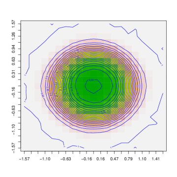
(a)

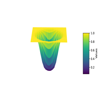
(b)

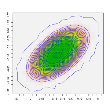
(c)

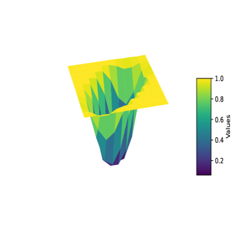
(d)

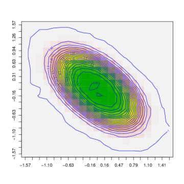
(e)

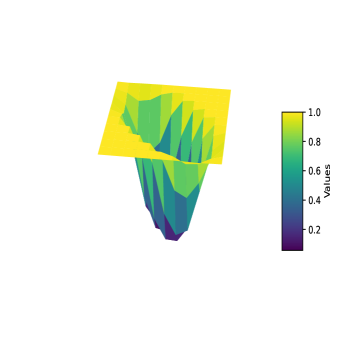
(f)

Figure 5. (A), (C), and (E) are contour plots; (B), (D), and (F) are corresponding surface plots of power under $H_{1t}$ when the location of the changepoint is considered at $k^{*}=\frac{n}{2},$ for von mises sine model with zero, positive, and negative association, respectively.

First, we consider the bivariate von Mises sine-model given in Equation-39. The plots are reported for three types of dependent data for this model. Since the value $\kappa_{3}$ decides the dependency between the random angles in this model, we keep $\kappa_{1}=\kappa_{2}=2$ throughout and vary $\kappa_{3}$. Figures 5(A) and 5(B) depict the power surface and the corresponding contour plot for independent data from the model given in Equation-39 with $\kappa_{3}=0$. Figures 5(C) and 5(D) depict the power surface and the corresponding contour plot for the data with right tilted association (positively dependent) from the model given in Equation-39 with $\kappa_{3}=2$. Figures 5(E) and 5(F) depict the power surface and the corresponding contour plot for the data with left tilted association (negatively dependent) from the model given in Equation-39 with $\kappa_{3}=-2$.

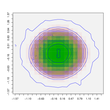
(a)

(b)

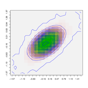
(c)

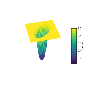
(d)

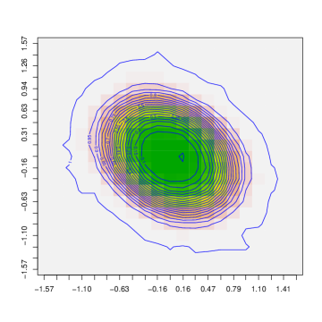
(e)

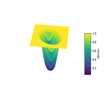
(f)

Figure 6. (A), (C), and (E) are contour plots; (B), (D), and (F) are corresponding surface plots of power under $H_{1t}$ when the location of the changepoint is considered at $k^{*}=\frac{n}{2},$ for von mises cos model with zero, positive, and negative association, respectively.

Next, we consider the bivariate von Mises cosine-model given in Equation-40. The plots are reported for three types of dependent data for this model. We keep $\kappa_{1}=\kappa_{2}=2$ for the data with no association (independent) and right-tilted association (positively dependent), $\kappa_{1}=\kappa_{2}=3$, for data with left-tilted association (negatively dependent) from the model and vary $\kappa_{3}$. Figures 6(A) and 6(B) depict the power surface and the corresponding contour plot for independent data from the model given in Equation-40 with $\kappa_{3}=0$. Figures 6(C) and 6(D) depict the power surface and the corresponding contour plot for positively dependent data from the model given in Equation-40 with $\kappa_{3}=2$. Figures 6(E) and 6(F) depict the power surface and the corresponding contour plot for negatively dependent data from the model given in Equation-39 with $\kappa_{3}=-1$.

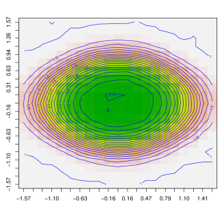
(a)

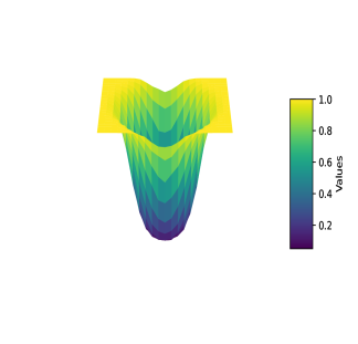
(b)

Figure 7. (A) is contour plot (B) is a corresponding surface plot of power under $H_{1t}$ when the location of the changepoint is considered at $k^{*}=\frac{n}{2},$ for the new toroidal distribution proposed by Biswas et al. (2024).

Finally, We considered the bivariate intrinsic model of toroidal distribution with the probability density function given in Equation-41 which is an independent distribution. Figures 7(B) and 7(C) depict the power surface and the corresponding contour plot for independent data from the model given in Equation-41 with $\kappa_{1}=\kappa_{2}=1,$ and $\nu=0.5$.

6.2. Spherical distributions

Here, we have considered the well-known spherical distribution, the bivariate Fisher distribution on the sphere due to Fisher (1953), and the probability density function can be found in Mardia, (2000, Ch. 9, pp. 168). Figure-4(B) displays a density plot of the distribution of the test statistic, $\mathcal{S}_{n}$ under $H_{0s}$ with the sample size of $n=1000$ from the independent bivariate Fisher distribution with $\kappa=2$, and different mean direction vectors such as, $(\mu_{\phi},\mu_{\theta})=(0,0),(\mu_{\phi},\mu_{\theta})=(0,\frac{\pi}{4}),(\mu_{\phi},\mu_{\theta})=(\frac{\pi}{2},0)$, and $(\mu_{\phi},\mu_{\theta})=(\frac{\pi}{2},\frac{\pi}{4})$. Although the Fisher distribution is widely used, some datasets do not fit well with the Fisher distribution and instead seem to originate from distributions with oval-shaped density contours. To address this, Kent (1982) proposed a model, with the density detailed in Mardia, (2000, Ch. 9, pp. 176). For $\kappa=5$ Figure-4(D) & 4(F) display the density plots of the distribution of the test statistic, $\mathcal{S}_{n}$ under $H_{0s}$ with the sample size of $n=1000$ from the independent bivariate Kent distribution with $\beta=3$, different mean direction vectors such as, $(\mu_{\phi},\mu_{\theta})=(0,0),(\mu_{\phi},\mu_{\theta})=(0,\frac{\pi}{6}),(\mu_{\phi},\mu_{\theta})=(\frac{2\pi}{3},0)$, and $(\mu_{\phi},\mu_{\theta})=(\frac{2\pi}{3},\frac{\pi}{6})$, and $\beta=-3$, different mean direction vectors such as, $(\mu_{\phi},\mu_{\theta})=(0,0),(\mu_{\phi},\mu_{\theta})=(0,\frac{\pi}{3}),(\mu_{\phi},\mu_{\theta})=(\frac{2\pi}{3},0)$, and $(\mu_{\phi},\mu_{\theta})=(\frac{2\pi}{3},\frac{\pi}{3})$, respectively.

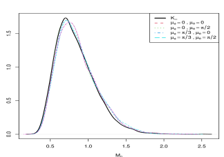
(a)

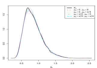
(b)

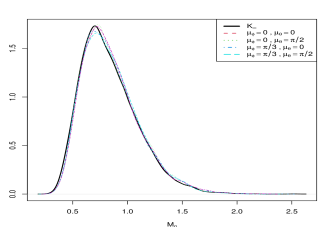
(c)

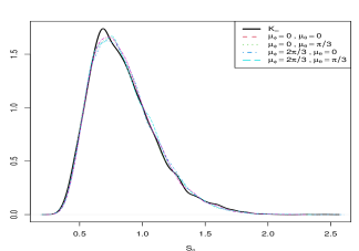
(d)

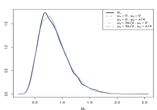
(e) von cos

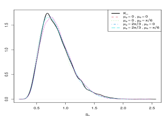
(f)

Figure 4. (A), (C), and (E) are the density plots of the test statistic, $\mathcal{M}_{n}$ under $H_{0t}$ with a sample of size $n=1000$ from von Mises sine model, von Mises cos model, and a new distribution proposed by Biswas et al. (2024), respectively. (B), (D), and (F) are the density plots of the test statistic, $\mathcal{S}_{n}$ under $H_{0s}$ with a sample of size $n=1000$ from Fisher distribution, Kent distribution with positive ovalness parameter, and Kent distribution with negative ovalness parameter, respectively.

$10^{4}$ iterations have been conducted for each of the above specifications. It is evident from Figure-4(B) that the densities of the distribution of the test statistics are nearly identical irrespective of the different mean direction vectors of Fisher distribution. Moreover, these are close to the density of the limiting distribution of the random variable $K_{\infty}$ (Equation-30). The same is observed in Figures 4(D) and 4(F) when the samples are drawn from the Kent distribution.

To generate the power surface and the corresponding contour, the location of the changepoint is considered at $k^{*}=\frac{n}{2},$ and the mean direction vector before the change is $(\mu_{\phi},\mu_{\theta})=(0,0).$ After the change a shift of $(\delta_{\phi},\delta_{\theta})$ in the mean direction vector is added to the initial one. Here, $\delta_{\phi}$ take $21$ equispaced values in $[-\frac{\pi}{2},\frac{\pi}{2}],$ and $\delta_{\theta}$ take $21$ equispaced values in $[-\frac{\pi}{2.5},\frac{\pi}{2.5}].$ We performed $10^{4}$ iterations to compute the power of the test statistic, $\mathcal{S}_{n}$ in Equation-38 for sample size of $n=500$ at the level of $5\%.$ Hence we obtain the surface and the corresponding contour plot out of it. These specifications have been implemented for different spherical distributions as follows.

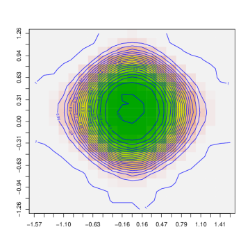
(a)

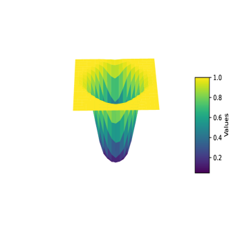
(b)

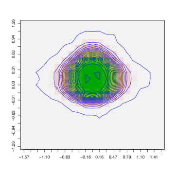
(c)

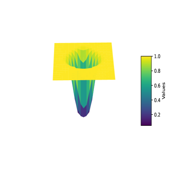
(d)

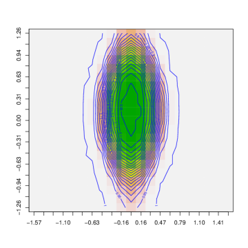
(e)

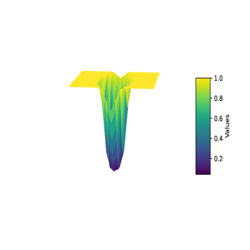
(f)

Figure 8. (A), (C), and (E) are contour plots; (B), (D), and (F) are corresponding surface plots of power under $H_{1s}$ when the location of the changepoint is considered at $k^{*}=\frac{n}{2},$ for Fisher distribution, Kent distribution with positive ovalness parameter, and Kent distribution with negative ovalness parameter, respectively.

First, we consider the bivariate Fisher distribution. Figures 8(A) and 8(B) depict the power surface and the corresponding contour plot for the concentration parameter $\kappa=2$. Next, for the concentration parameter, $\kappa=5$ and ovalness parameters $\beta=3$ to obtain Figures-8(C), 8(D). Similarly Figures-8(E), 8(F) show the power surface and the corresponding contour plot with ovalness parameters $\beta=-3$.

7. Data Analysis

Data of Biporjoy cyclone: The Extremely Severe Cyclonic Storm “Biparjoy” over the east-central Arabian Sea occurred from 6th June to 19th June 2023, severely affecting some states of western India. According to the report by the Regional Specialized Meteorological Center - tropical cyclones, New Delhi India Meteorological Department (IMD) (see, https://mausam.imd.gov.in/Forecast/mcmarq/mcmarq_data/cyclone.pdf) this cyclone was longest duration cyclone since 1977. Cyclone Biparjoy, a very severe cyclonic storm in June 2023, exemplified the intricate interplay between wind direction and wave direction during its course over the Arabian Sea. Originating from a low-pressure area, Biparjoy intensified and reached peak wind speeds of 195 km/h (121 mph), which played a crucial role in wave formation. These intense winds imparted substantial energy to the ocean’s surface, producing large and powerful waves, resulting in severe coastal flooding and erosion, particularly along the Gujarat coast. This surge, along with the powerful waves, caused extensive damage to coastal infrastructure and ecosystems, highlighting the storm’s destructive potential.

An upper air cyclonic circulation formed over the Southeast Arabian Sea and developed into a depression early on June 6. It moved northwards, intensifying into a deep depression and then into Cyclonic Storm “Biparjoy” in the adjoining Southeast Arabian Sea. Continuing its northward trajectory, it intensified into a Severe Cyclonic Storm (CS) over the east-central Arabian Sea and further into a Very Severe Cyclonic Storm (VSCS) in the same region. From June 7 to 11, Biparjoy followed a recurving path, moving gradually north-northwestwards, then north-northeastwards, and finally northwards. As it moved northwards, it intensified into an Extremely Severe Cyclonic Storm (ESCS) over the east-central Arabian Sea. It then shifted north-northeastwards briefly before returning to a northward path, maintaining its intensity as an ESCS. Subsequently, it moved north-northwestwards and weakened into a VSCS over the northeast and adjoining east-central Arabian Sea. Continuing its north-northwestward, then northward, and finally northeastward movement, the storm gradually weakened. It crossed the Saurashtra and Kutch regions of India and the adjoining Pakistan coasts between Mandvi (Gujarat) and Karachi (Pakistan), near latitude $23.28^{\circ}N$ and longitude $68.56^{\circ}E$. After landfall, Biparjoy moved east-northeastwards, weakening into a cyclonic storm over Saurashtra and Kutch. It then moved northeastwards and weakened into a deep depression over Southeast Pakistan and adjoining Southwest Rajasthan and Kutch. Continuing its east-northeastward movement, it further weakened into a depression over South Rajasthan and adjoining north Gujarat and eventually into a well-marked low-pressure area over central Northeast Rajasthan and its surroundings by the morning of June 19. The cyclone altered its course approximately nine times during its journey, traversing a distance of 2525 kilometers. This frequent change in direction made it particularly challenging to forecast the path of the cyclone.

Intending to study the possible association of the wind direction and wave direction at a chosen location with the meteorological events described above, we collected the 10-meter-above-the-sea-level wind direction and mean wave direction data (see Hersbach et al., 2023) at the location with coordinates $17.3^{\circ}N$, and $67.3^{\circ}E$, which is about 1200 km from the location of the landfall. The hourly data spans from June 1, 2020, 0000 UTC to June 20, 2023, 1200 UTC. This resulted in a total of 360 observations reported in degrees. As discussed above, several significant meteorological events happened during the period 6th - 19th June 2023, which indicates the possibility of changepoints being present in the data. Since the mean direction is unknown, we executed the test for the toroidal mean direction to determine the existence of changepoints for mean direction in this data set. The initial mean direction of the data has been estimated using the first $25\%(\lambda\%)$ of the entire data. Subsequently using the method developed in Section 4 and the binary segmentation procedure, we found the presence of multiple changepoints. Table-1 reports the results. It may be noted that we used the limiting distributions $K_{\infty}$ to obtain the corresponding p-values. We also represent the data using a circular temporal plot in Figure-9(A) & (B) where five annular circles from the center to outward represent the corresponding estimated changepoints in the mean direction of the wind and wave direction, respectively. The segment-wise estimated mean is represented by blue, and magenta bubble plots at the outer end of the corresponding segment.

We collected latitude and longitude data for the path of the Biporjoy cyclone, considering the spherical nature typical of cyclone paths. The data spans quarterly observations from June 6, 2020, 0000 UTC, to June 19, 2023, 1200 UTC, totaling 97 observations in degrees. Given significant meteorological events between June 6-19, 2023, suggesting potential changepoints, we conducted tests on the spherical mean direction to detect these changepoints. The initial mean direction of the data has been estimated using the first $25\%(\lambda\%)$ of the entire data. Subsequently using the method developed in Section 5 and the binary segmentation procedure, we identified multiple changepoints, as detailed in Table 2. Notably, we utilized the limiting distributions $K_{\infty}$ to derive corresponding p-values for our analysis. We also represent the data using a circular temporal plot in Figure 10(A) & (B) where five annular circles from the center to outward represent the corresponding estimated changepoints in the mean direction of the latitude and longitude, respectively. The segment-wise estimated mean is represented by blue, and magenta bubble plots at the outer end of the corresponding segment.

Data segment	Estimated changepoint	P-value
1-360	122	0.0000
1-122	56	0.0000
57-122	115	0.0008
123-360	284	0.0000
123-284	183	0.0000
285-360	325	0.0000

Table 1. Some significant changepoints using the binary segmentation scheme for the wind-wave direction data of Biporjoy cyclone .

Data segment	Estimated changepoint	P-value
1-97	77	0.0000
1-77	26	0.0000
27-77	55	0.0002
78-97	88	0.0009

Table 2. Some significant changepoints using the binary segmentation scheme for the direction of the path of the Biporjoy cyclone

8. Conclusion

It has been discovered that the characteristics of the underlying distribution abruptly change at unknown instances in many temporally ordered data sets. Finding this kind of instance is crucial for a lot of applications. Although this subject has been extensively researched for linear data, bivariate angular data has received no attention so far. The changepoint problems for the mean direction of bivariate angular data (spherical and toroidal) are examined for the first time in the literature. The concept of the “square” of an angle has been introduced using the intrinsic geometry of a curved torus. Analogous to the dispersion matrix for bivariate linear random variables, the “curved dispersion matrix” for bivariate angular random variables is introduced. Using this analogous measure of the “Mahalanobis distance,” we develop two new non-parametric tests to identify changes in the mean direction parameters for toroidal and spherical distributions. The limiting distributions of the test statistics have been derived, and their power surface and contours have been obtained through extensive simulation. The proposed methods have been put into practice to identify the changepoints in the path of the cyclonic storm “Biporjoy” and identify changepoints in mean direction for hourly wind-wave direction observations.

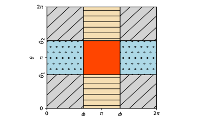
(a)

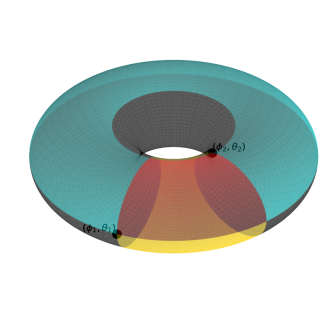
(b)

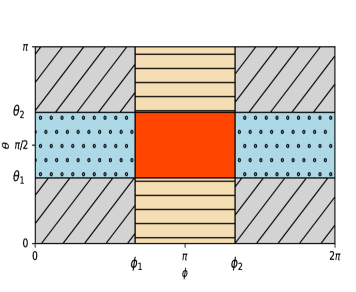
(c)

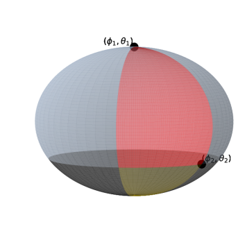
(d)

Figure 3. Area between $(\phi_{1},\theta_{1})$, and $(\phi_{2},\theta_{2})$ (A) flat torus, (B) curved torus, (C) flat sphere, (D) sphere.

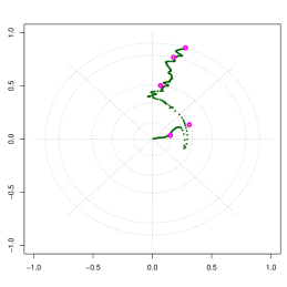
(a)

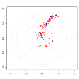
(b)

Figure 9. The circular temporal plot of (A) wave direction, and (B) wind direction of the Super Cyclonic Storm (SuCS) “BIPORJOY”

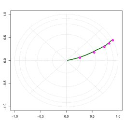
(a)

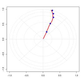
(b)

Figure 10. The circular temporal plot of (A) latitude, and (B) longitude of the path of the Super Cyclonic Storm (SuCS) “BIPORJOY”.

References

- Anastasiou and Papanastasiou (2023) A. Anastasiou and A. Papanastasiou. Generalized multiple change-point detection in the structure of multivariate, possibly high-dimensional, data sequences. Statistics and Computing, 33(5):94, 2023.
- Antoch et al. (1997) J. Antoch, M. Husková, and Z. Prásková. Effect of dependence on statistics for determination of change. Journal of Statistical Planning and Inference, 60:291–310, 1997.
- Banerjee and Mazumder (2018) B. Banerjee and S. Mazumder. A more powerful test identifying the change in mean of functional data. Annals of the Institute of Statistical Mathematics, 70:691–715, 2018.
- Banerjee et al. (2020) B. Banerjee, A. K. Laha, and A. Lakra. Data-driven dimension reduction in functional principal component analysis identifying the change-point in functional data. Statistical Analysis and Data Mining: The ASA Data Science Journal, 13(6):529–536, 2020.
- Billingsley (2013) P. Billingsley. Convergence of probability measures. John Wiley & Sons, 2013.
- Biswas and Banerjee (2024) S. Biswas and B. Banerjee. Exploring uniformity and maximum entropy distribution on torus through intrinsic geometry: Application to protein-chemistry. arXiv preprint arXiv:2405.09149, 2024.
- Biswas et al. (2024) S. Biswas, B. Banerjee, and A. K. Laha. Changepoint problem with angular data using a measure of variation based on the intrinsic geometry of torus. arXiv preprint arXiv:2403.00508, 2024.
- Cobb (1978) G. Cobb. The problem of the nile: Conditional solution to a change-point problem. Biometrika, 65:243–251, 1978.
- Davis et al. (1995) R. Davis, D. Huang, and Y.-C. Yao. Testing for a change in the parameter values and order of an autoregressive model. The Annals of Statistics, 23:282–304, 1995.
- Fisher (1953) R. A. Fisher. Dispersion on a sphere. Proceedings of the Royal Society of London. Series A. Mathematical and Physical Sciences, 217(1130):295–305, 1953.
- Gallier and Quaintance (2020) J. Gallier and J. Quaintance. Differential Geometry and Lie Groups:A Computational Perspective. Springer, 2020.
- Ghosh et al. (1999) K. Ghosh, S. R. Jammalamadaka, and M. Vasudaven. Change-point problems for the von mises distribution. Journal of Applied Statistics, 26(4):423–434, 1999.
- Grabovsky and Horváth (2001) I. Grabovsky and L. Horváth. Change-point detection in angular data. Annals of the Institute of Statistical Mathematics, 53:552–566, 2001.
- Hersbach et al. (2023) H. Hersbach, B. Bell, P. Berrisford, G. Biavati, A. Horányi, J. Muñoz Sabater, C. Nicolas, J.and Peubey, R. Radu, I. Rozum, D. Schepers, A. Simmons, C. Soci, D. Dee, and J.-N. Thépaut. Era5 hourly data on single levels from 1940 to present. Copernicus Climate Change Service (C3S) Climate Data Store (CDS), DOI: 10.24381/cds.adbb2d47 (Accessed on 10-January-2023):268–279, 2023. URL https://cds.climate.copernicus.eu/cdsapp#!/dataset/reanalysis-era5-single-levels?tab=overview.
- Hörmann and Kokoszka (2010) S. Hörmann and P. Kokoszka. Weakly dependent functional data. The Annals of Statistics, 38(3):1845–1884, 2010. ISSN 0090-5364. doi: 10.1214/09-AOS768. URL http://dx.doi.org/10.1214/09-AOS768.
- Horváth and Kokoszka (2012) L. Horváth and P. Kokoszka. Inference for functional data with applications, volume 200. Springer Science & Business Media, 2012.
- Horváth et al. (1999) L. Horváth, P. Kokoszka, and J. Steinebach. Testing for changes in multivariate dependent observations with applications to temperature changes. Journal of Multivariate Analysis, 68:96–119, 1999.
- Kent (1982) J. T. Kent. The fisher-bingham distribution on the sphere. Journal of the Royal Statistical Society: Series B (Methodological), 44(1):71–80, 1982.
- Kirch et al. (2015) C. Kirch, B. Muhsal, and H. Ombao. Detection of changes in multivariate time series with application to eeg data. Journal of the American Statistical Association, 110(511):1197–1216, 2015.
- Kokoszka and Leipus (2000) P. Kokoszka and R. Leipus. Change-point estimation in arch models. Bernoulli, 6:513–539, 2000.
- Ley and Verdebout (2017) C. Ley and T. Verdebout. Modern directional statistics. Chapman and Hall/CRC, 2017.
- Lombard (1986) F. Lombard. The change–point problem for angular data: A nonparametric approach. Technometrics, 28(4):391–397, 1986.
- Mardia (2000) K. V. Mardia. Directional statistics. New York: John Wiley and Sons., 2000.
- Mardia et al. (2000) K. V. Mardia, P. E. Jupp, and K. Mardia. Directional statistics, volume 2. Wiley Online Library, 2000.
- Mardia et al. (2007) K. V. Mardia, C. C. Taylor, and G. K. Subramaniam. Protein bioinformatics and mixtures of bivariate von mises distributions for angular data. Biometrics, 63(2):505–512, 2007.
- SenGupta and Laha (2008) A. SenGupta and A. K. Laha. A likelihood integrated method for exploratory graphical analysis of change point problem with directional data. Communications in Statistics-Theory and Methods, 37(11):1783–1791, 2008.
- Shao and Zhang (2010) X. Shao and X. Zhang. Testing for change points in time series. Journal of the American Statistical Association, 105(491):1228–1240, 2010.
- Singh et al. (2002) H. Singh, V. Hnizdo, and E. Demchuk. Probabilistic model for two dependent circular variables. Biometrika, 89(3):719–723, 2002.