Insights from the exact analytical solution of periodically driven transverse field Ising chain

Abstract

We derive an exact analytical expression, at stroboscopic intervals, for the time-dependent wave function of a class of integrable quantum many-body systems, driven by the periodic delta-kick protocol. To investigate long-time dynamics, we use the wave-function to obtain an exact analytical expression for the expectation value of defect density, magnetization, residual energy, fidelity, and correlation function after the $n$th drive cycle. Periodically driven integrable closed quantum systems absorb energy, and the long-time universal dynamics are described by the periodic generalized Gibbs ensemble(GGE). We demonstrate that the expectation values of all observables are divided into two parts: one highly oscillatory term that depends on the drive cycle $n$, and the rest of the terms are independent of it. Typically, the $n$-independent part constitutes the saturation at large $n$ and periodic GGE. The contribution from the highly oscillatory term vanishes in large $n$.

I Introduction

In recent years, there has been significant research into the physics of closed quantum systems driven out of equilibrium, both theoretically[1, 2, 3, 4, 5, 6, 7, 8] and experimentally[9, 10, 11, 12, 13]. These studies have used a variety of experimental setups, including ultracold atoms, ion traps, semiconductor qubits, and superconducting qubits. Initial research in this field focused on sudden quench and ramp protocols, but there is now an increased interest in periodically driven systems[14, 15, 16, 17]. The ability to modify and control material properties using optical pulses has gathered significant interest from the scientific community due to its potential application in technology[18, 19, 20, 21, 22, 23]. Floquet theory makes it easier to describe such systems at discrete time intervals by using a time-independent Floquet Hamiltonian derived from the time evolution operator over one time period. This approach has resulted in the emergence of Floquet engineering as a novel research area. Advances in Floquet engineering have enabled the preparation of systems in different equilibrium phases and uncover new non-equilibrium phases and also the transitions between them. Recently, Floquet theory reveals a number of distinct phenomena in these systems that do not occur in equilibrium or other driven systems. Dynamical localization[24, 25, 26] and freezing[27, 28, 29, 30, 31], dynamical transitions[32, 33], Floquet topological phases[34, 36, 35, 37, 38, 39], Floquet realization of quantum scars[40, 41, 42, 43, 44], time-crystalline states of matter, and the optically controlled materials, are just a few examples. These phenomena make periodically driven systems an dynamic field of research, yielding new insights into how time-periodic drives can fundamentally alter system behavior and properties.
In this study, we investigate the non-equilibrium dynamics of a periodically driven quantum integrable system using a semi-analytical method. While most analytical approaches for periodically driven systems rely on Floquet theory, which assumes an infinite duration for the periodic drive (i.e.,$n\to\infty$), this is not practical in experimental settings. Nevertheless, it is expected that for sufficiently large $n$, experimental results should match with those predicted by Floquet theory. Recent advances in ultrafast laser science have provided a unique opportunity to investigate Floquet engineering with extremely high time resolution, allowing one to study periodically driven states on shorter time scales[20, 21]. For finite $n$, most calculations are typically performed numerically. Our goal is to bridge this gap by deriving an analytical expression for the time-dependent wavefunction of a periodically driven system after finite $n$ drive cycles. Our results are exact and valid for any finite $n$ and drive frequency $\omega$, enables experimentalists to verify their findings without relying on Floquet theory. Additionally, we provide an analytical expression for the expectation values of several widely studied observables found in the literature, after $n$ periods. To our knowledge, this kind of extensive analytical exact expression for periodically driven quantum many-body systems has not been reported before.
This formulation applies to any experimentally realizable system that can be simplified to a quantum two-level system. It can also be extended to a class of exactly solvable models that can be expressed in the following form:

$$H = \sum_{k}\psi_{k}^{\dagger}\left[(g(t)-a_{k})\sigma^{3}+b_{k}\sigma^{1}\right]\psi_{k},$$ (1)

where, example Hamiltonian includes models such as the transverse field Ising (TFI) chain, the quantum XY chain, the Kitaev chain in one dimention(1D), and the Kitaev model in 2D. Here, $a_{k}$ and $b_{k}$ are functions of momentum only, and $g(t)$ is the time-dependent parameter varied according to a time-periodic protocol. $\sigma^{1}$ and $\sigma^{3}$ are Pauli matrices, and $\psi_{k}^{\dagger}=(c_{k}^{\dagger},c_{-k})$, where $c_{k}$ is the fermionic annihilation operator in momentum space, given by

$$c_{k}=\frac{1}{\sqrt{L}}\sum_{j=1}^{L}e^{ikj}c_{j}$$ (2)

and $L$ is total number of fermions. In this paper we will focus solely on the 1D TFI chain for clarity.
Although this formulation can be applied to any periodic drive protocol, provided the evolution operator for one time period can be exactly known analytically, we restrict our calculations to the periodically kicked drive protocol for calculational simplicity. Our upcoming work will involve calculations with square pulse drive protocol. For a sinusoidal drive protocol, it is possible to either find the analytical expression for the evolution operator over one time period using the adiabatic-impulse-adiabatic approximation or compute it numerically by solving the time-dependent Schrödinger equation. Once the evolution operator for one time period is known, our formulation can also be extended to sinusoidal drive protocols. Additionally, this approach can also be adapted to some non-Hermitian systems, which have recently attracted significant interest[45].
The main results of our study are as follows. We derive an exact analytical expression for the time-dependent wavefunction after $n$ drive cycles. Using this expression, we obtain an analytical formula for the expectation value of the defect produced after $n$ drive cycles. Additionally, we calculate the analytical expressions for residual energy, magnetization, and fidelity. Furthermore, we provide the exact expression for all two-point correlators. Using these results, we numerically compute the entanglement entropy, which is consistent with results available in the literature. Our expressions have streamlined the numerical calculations and reduced the time needed for determining the entanglement entropy and other observables for our driven system.
The paper is organized as follows: In Sec. II, we provide a brief introduction to the system of interest, the transverse field Ising (TFI) chain Hamiltonian, and review some of its key properties. We also introduce the periodic drive protocol and derive the analytical expression for the stroboscopic time-dependent state after any arbitrary $n$ drive cycles. Using this expression, we derive the formula for the residual energy in Sec. III and discuss its properties. In Sec. IV, we derive the expression for magnetization and explore the concept of dynamical freezing. Sec. V we present the expression for fidelity and discuss it’s properties. We discuss all two point correlators in Sec. VI. Finally, we discuss our results and conclude in Sec. VII. Details of the calculations for determining the $n$th power of the evolution matrix are provided in the Appendix IX.

II Model Hamiltonian

In this section, we will review the exactly solvable model required for our discussion on periodic drive. To simplify calculations, we have chosen one-dimensional free-fermionic TFI chain for this paper. We have discussed some of the important properties of the model followed by the details of our drive protocol. Next we provide an analytic expression for driven wavefunction, followed by analytic expression for defect density.

II.1 Transeverse-field Ising chain Hamiltonian

To begin, let us briefly discuss the model: a spinless, free fermionic one-dimensional transverse-field Ising (TFI) chain with $L$ sites. The time-independent Hamiltonian of this model is given by:

$$H=-J\sum_{i=1}^{L}\left(\sigma_{i}^{x}\sigma_{i+1}^{x}+g_{0}\sigma_{i}^{z}\right),$$ (3)

where, $\sigma_{i}^{\alpha}$ denotes the Pauli spin matrices at site $i$, $J$ is the strength of the nearest-neighbor Ising interaction, and $g_{0}$ is the strength of the transverse field. The Ising Hamiltonian can be transformed into a quadratic free fermionic Hamiltonian using a non-local Jordan-Wigner transformation:

$$\sigma_{i}^{z} = 1-2c_{i}^{\dagger}c_{i},$$ (4)

$$\sigma_{i}^{x} = -(c_{i}+c_{i}^{\dagger})\prod_{j<i}(1-2c_{j}^{\dagger}c_{j}),$$ (5)

where, $c_{i}$ is the fermionic annihilation operator at site $i$. Utilizing translational invariance, the quadratic fermionic Hamiltonian in momentum space can be expressed as $H=\sum_{k}\psi_{k}^{\dagger}H_{k}\psi_{k}$, with:

$$H_{k}=(g_{0}-\cos k)\sigma^{3}+(\sin k)\sigma^{1},$$ (6)

and $k=\pm\frac{1}{2}\frac{2\pi}{L},\ldots,\pm\frac{L-1}{2}\frac{2\pi}{L}$. For simplicity, we set $J=1$ for all calculations, and all comparisons are made in units of $J$. The total Hilbert space of the Hamiltonian is a product of two-dimensional subspaces spanned by $|0_{k},0_{-k}\rangle$ and $|1_{k},1_{-k}\rangle$ for each $k$ mode. The Hamiltonian in momentum space can be diagonalized using the Bogoliubov transformation:

$$c_{k}=u_{k}\gamma_{k}+v_{-k}^{*}\gamma_{k}^{\dagger}.$$ (7)

The final Hamiltonian in the Bogoliubov basis can be written as:

$$H=\sum_{k>0}\epsilon_{k}\left(\gamma_{k}^{\dagger}\gamma_{k}-\frac{1}{2}\right),$$ (8)

where, the eigenvalues are $\pm\epsilon_{k}$, with:

$$\epsilon_{k}=\sqrt{(g_{0}-\cos k)^{2}+\sin^{2}k},$$ (9)

and the eigenvectors are:

$$\left(\begin{array}[]{c}u_{k}\\ v_{k}\end{array}\right)=\left(\begin{array}[]{c}\cos\frac{\phi_{k}}{2}\\ \sin\frac{\phi_{k}}{2}\end{array}\right),$$ (10)

where, $\tan\phi_{k}=\frac{\sin k}{g_{0}-\cos k}$. The system becomes gapless at $k=0$ or $k=\pi$ and $g_{0}=\pm 1$ indicates the presence of a quantum critical point[46]. The Hamiltonian can be made time-dependent by allowing $g_{0}$ to vary with time, i.e., $g_{0}=g(t)$. For a time-dependent parameter $g(t)$, the Hamiltonian in momentum space is given by:

$$H_{k}(t)=(g(t)-\cos k)\sigma^{3}+(\sin k)\sigma^{1}.$$ (11)

The non-equilibrium dynamics of the model can be studied by solving the time-dependent Schrödinger equation

$$i\partial_{t}|\psi_{k}\rangle=H_{k}(t)|\psi_{k}\rangle$$ (12)

for each mode $k$. We are particularly interested in a special category of driven systems where the parameter $g(t)$ varies periodically over time, that is, $g(t)=g(t+T)$, where $T$ is the period of the driving protocol. We further simplify the driving protocol by assuming the transverse field is periodically modulated by delta pulse kicks with frequency $\omega$, given by

$$g(t)=g_{0}+g_{1}\sum_{s=-\infty}^{\infty}\delta(t-sT),$$ (13)

where $T=\frac{2\pi}{\omega}$ and $s$ is an integer. The periodic drive makes the Hamiltonian time-dependent, such that $H(t+T)=H(t)$. The stroboscopic time evolution operator over one period for such a time-periodic Hamiltonian, can be written as

$$U_{k}(T)=\mathbb{T}\exp\left(-i\int_{0}^{T}H(t)\,dt\right)=\exp\left(-iH_{k}^{F}T\right),$$ (14)

where $H_{k}^{F}$ is the time-independent Floquet Hamiltonian and $\mathbb{T}$ is the time ordered product. Calculating the Floquet Hamiltonian is generally quite difficult because of the complex time-ordering involved. As a result, the majority of research on periodically driven systems has concentrated on obtaining the Floquet Hamiltonian through various approximation methods. It is important to note that our calculations do not rely on the Floquet Hamiltonian and are also applicable in cases where the analytic expression for the Floquet Hamiltonian is unknown. For the delta-kicked drive protocol, the symmetrized time-evolution operator is given by[47, 48]

$$U_{k}(T)=e^{-i\frac{g_{1}}{2}\sigma^{3}}e^{-iT\left[(g_{0}-\cos k)\sigma^{3}+(\sin k)\sigma^{1}\right]}e^{-i\frac{g_{1}}{2}\sigma^{3}},$$ (15)

which simplifies to

$$U_{k}(T)=\begin{pmatrix}\alpha_{k}&-\beta_{k}^{*}\\ \beta_{k}&\alpha_{k}^{*}\end{pmatrix},$$ (16)

where,

$$\alpha_{k} = e^{-ig_{1}}\left(\cos(\Phi_{k})-in_{kz}\sin(\Phi_{k})\right),$$ (17)

$$\beta_{k} = -in_{kx}\sin(\Phi_{k}),$$ (18)

$$\Phi_{k} = T\epsilon_{k},$$ (19)

$$n_{kz} = \frac{g_{0}-\cos k}{\epsilon_{k}},$$ (20)

$$n_{kx} = \frac{\sin k}{\epsilon_{k}}.$$ (21)

Eq. (16) is the starting point of extending our calculation to other drive protocol.

II.2 Time-dependent state after $n$th period

In this subsection we derive time dependent state after $n$th period, where $n$ is a positive integer. Using time evolution operator, one can determine the wave function after $n$ periods as,

$$|\psi_{k}(t=nT)\rangle=U_{k}^{n}(T)|\psi_{k}(t=0)\rangle.$$ (22)

With an analytical expression for the evolution operator over one time period, one can easily compute the $n$th power of the $2\times 2$ matrix after a few lines of algebra (see details in the Appendix). Using the properties of SU(2) matrix, the $n$th power of the time evolution operator is given by[49]

$$U_{k}^{n}(T) = U_{k}(T)\cdot\mathcal{F}_{n-1}(\xi_{k})-\mathbb{I}_{2}\cdot\mathcal{F}_{n-2}(\xi_{k}),$$ (23)

$$\xi_{k} = \frac{1}{2}\text{Tr}(U_{k}(T))=\mathfrak{Re}[\alpha_{k}],$$ (24)

where $\mathcal{F}_{n}(x)$ denotes the Chebyshev polynomials of the second kind of degree $n$ in $x$, and $\mathbb{I}_{2}$ is the $2\times 2$ identity matrix. The time-dependent state after $n$ drive periods can be expressed in terms of the initial state and other Hamiltonian parameters as

$$\left(\begin{array}[]{c}u_{k}(n)\\ v_{k}(n)\end{array}\right) = \left(\begin{array}[]{cc}\alpha_{k}\mathcal{F}_{n-1}(\xi_{k})-\mathcal{F}_{n-2}(\xi_{k})&-\beta_{k}^{*}\mathcal{F}_{n-1}(\xi_{k})\\ \beta_{k}\mathcal{F}_{n-1}(\xi_{k})&\alpha_{k}^{*}\mathcal{F}_{n-1}(\xi_{k})-\mathcal{F}_{n-2}(\xi_{k})\end{array}\right)\left(\begin{array}[]{c}u_{k}(0)\\ v_{k}(0)\end{array}\right).$$ (31)

For simplicity, let us consider the initial state is a product state, $|\psi(t=0)\rangle=\prod_{k}\left(0,1\right)^{\text{T}}$. While an analytic solution can be found for any initial state, this particular initial state simplifies the calculations. In this limit, $u_{k}(n)$ and $v_{k}(n)$ simplify to,

$$u_{k}(n) = -\beta_{k}^{*}\mathcal{F}_{n-1}(\xi_{k})=-in_{kx}\sin\Phi_{k}\frac{\sin n\theta_{k}}{\sin\theta_{k}},$$ (32)

$$v_{k}(n) = \alpha_{k}^{*}\mathcal{F}_{n-1}(\xi_{k})-\mathcal{F}_{n-2}(\xi_{k})$$ (33)

$$= \cos n\theta_{k}+i\mathfrak{Im}[\alpha_{k}^{*}]\frac{\sin n\theta_{k}}{\sin\theta_{k}}.$$

Here, we have used the property of Chebyshev polynomials of the second kind: $\mathcal{F}_{n}(x)=\frac{\sin(n+1)\theta}{\sin\theta}$ with $x=\cos\theta$. Note that $\theta_{k}$, appearing in the equation

$$\theta_{k}=\cos^{-1}\xi_{k}=\cos^{-1}(\cos g_{1}\cos\Phi_{k}-n_{kz}\sin g_{1}\sin\Phi_{k}),$$ (34)

represents the eigenvalues $\exp(i\theta_{k})$ of the evolution operator $U_{k}(T)$ given in Eq.(16). Equations (32, 33) constitute significant exact analytical results that have been verified with exact numerics. Almost similar results for two-level system are also obtained in[32, 50]. In the rest of this paper, we will use these expressions to provide analytical expressions for the expectation values of several commonly studied observables in the literature. Finally, before conclusion, please note that obtaining exact and analytical solutions for a periodically driven integrable many-body system in arbitrary parameter regimes remains challenging using nonperturbative methods. Decoupling of the total Hilbert space into independent $k$ modes simplifies our task here.

II.3 Defect-denisty

In this subsection, we calculate the excitation probability, which is essentially the overlap of the time dependent state with the excited state of the two-level system at $t=0$ for each value of $k$. For quench and ramp protocol, defect density at final state show universal Kibble-Zurek scaling[51, 52, 53, 54]. Using the exact wave function, the excitation probability after $n$ drive cycles[55, 56] is defined as

$$p_{k}(n)=|\langle(1,0)|\psi_{k}(n)\rangle|^{2}=|u_{k}(n)|^{2}.$$ (35)

This is given by

$$|u_{k}(n)|^{2}=\frac{\Gamma_{k}^{2}}{2}\left(1-\cos 2n\theta_{k}\right),\quad\Gamma_{k}=\frac{n_{kx}\sin\Phi_{k}}{\sin\theta_{k}},$$ (36)

where $\Gamma_{k}$ depends on the $n_{kx},\Phi_{k}$ and $\theta_{k}$ as defined in the previous section. The above expression is a product of two terms: one highly oscillatory term $\cos 2n\theta_{k}$ coming from the Chebyshev polynomials of order $n-1$, and the other term, $\Gamma_{k}$, which varies slowly with $k$. We have plotted this expression in Fig. (1(a)) as a function of $k$ for $n=15$, with the slowly varying term $\Gamma_{k}$ shown in orange. The number of drive cycles $n$ influences the oscillatory behavior, with a higher $n$ leading to more oscillations. The wave function after $n$ drive cycles is related to the Chebyshev polynomials of degrees $n-1$ and $n-2$. Since the Chebyshev polynomial of order $n$ has $n$ roots, increasing $n$ results in more oscillations in the wave function. Similarly, one can find an expression for $|v_{k}(n)|^{2}$, as the sum of $|u_{k}(n)|^{2}$ and $|v_{k}(n)|^{2}$ must add up to unity to maintain normalization.

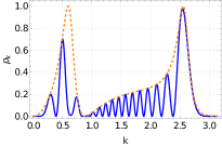
(a)  

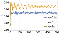
(b)  

Figure 1: (a) The behavior of $|u_{k}(n)|^{2}$ as a function of $k$ for $n=15$, plotted as a solid blue line. Higher $n$ corresponds to more oscillations. The slowly varying function $\Gamma_{k}^{2}/2$ is shown as a dashed orange line. (b) The total defect generated after $n$ cycles is plotted against $n$ for different frequencies. The dashed red line for $\omega=0.1\pi$ represents the saturation value for large $n$, computed using Eq. (38). Parameters used: $L=2048$, $g_{0}=2$, $g_{1}=0.5$.

Using Eq. (36), we can also calculate the total defect $n_{d}(n)$ generated after $n$ drive cycles, given by

$$n_{d}(n)=\frac{1}{L}\sum_{k>0}p_{k}(n)=\frac{1}{L}\sum_{k>0}\frac{\Gamma_{k}^{2}}{2}\left(1-\cos 2n\theta_{k}\right).$$ (37)

This sum cannot be evaluated analytically, so we resort to numerical evaluation. Figure 1(b) shows the total defect $n_{d}$ as a function of $n$ for different frequencies, with the defect saturating at large $n$. The saturation value can be calculated using the slowly varying function $\Gamma_{k}^{2}/2$ and is given by

$$n_{d}^{sat}=\frac{1}{L}\sum_{k>0}\frac{\Gamma_{k}^{2}}{2}=\frac{1}{L}\sum_{k>0}\left(\frac{n_{kx}\sin\Phi_{k}}{\sin\theta_{k}}\right)^{2}.$$ (38)

Note that the only terms containing the drive frequency $\omega$ in the above expression is $\Phi_{k}=\frac{2\pi\epsilon_{k}}{\omega}$ and $\theta_{k}$ that involves $\Phi_{k}$. At large $\omega$, $\sin^{2}\Phi_{k}$ approaches zero, $\theta_{k}\sim g_{1}$, implying that $n_{d}^{sat}$ becomes nearly zero. Physically, this means that at high frequencies, the system fails to respond to the external drive and remains close to the initial state, resulting in zero defect. Additionally, at $g_{1}=0$ and $\omega=2\pi$, i.e., $T=1$, we have $\theta_{k}=\Phi_{k}=\epsilon_{k}$, which simplifies the saturation value of the defect density to

$$n_{d}^{sat}=\frac{1}{L}\sum_{k>0}\frac{1}{1+\left(\frac{g_{0}-\cos k}{\sin k}\right)^{2}}=\frac{1}{4g_{0}^{2}}.$$ (39)

III Residual energy

In the previous section, we derived the expression for the defect generated due to energy absorption from the external drive. In this section, we focus on the residual energy after $n$ drive cycles, which determines the amount of energy absorbed by the system from an external drive. The residual energy is defined as the additional energy per site in the time-dependent state as compared to the ground state. Understanding the behavior of the residual energy is also crucial as it displays universal scaling of quantum systems near the critical point. Additionally, for periodically driven integrable systems, it has been shown that the zeros of the rate function in the work distribution statistics are related to the residual energy, enabling more accurate experimental measurements[56].
We define the residual energy as

$$E_{res}=\frac{1}{L}\sum_{k}\left(\epsilon_{k}(n)-\epsilon_{k}(0)\right),$$ (40)

where $\epsilon_{k}(n)=\langle\psi_{k}(nT)|H_{k}^{0}|\psi_{k}(nT)\rangle$ and $H_{k}^{0}$ is the initial Hamiltonian. Using the wavefunction expression from Eq. (31), the analytical expression for the residual energy and its large $n$ saturation value are given by

$$E_{res}(n) = \frac{1}{L}\sum_{k>0}\left[\Gamma_{k}^{2}(g_{0}-\cos k)+\Gamma_{k}^{2}\left(\sin g_{1}\cos\Phi_{k}+n_{kz}\cos g_{1}\sin\Phi_{k}-g_{0}+\cos k\right)\cos 2n\theta_{k}\right]$$ (41)

$$-\frac{\Gamma_{k}\sin k}{\sin\theta_{k}}\left(\sin g_{1}\cos\Phi_{k}+n_{kz}\cos g_{1}\sin\Phi_{k}\right),$$

$$E_{res}^{sat} = \frac{1}{L}\sum_{k>0}\left[\Gamma_{k}^{2}(g_{0}-\cos k)-\frac{\Gamma_{k}\sin k}{\sin\theta_{k}}\left(\sin g_{1}\cos\Phi_{k}+n_{kz}\cos g_{1}\sin\Phi_{k}\right)\right].$$ (42)

We have plotted the residual energy from Eq. (41) as a function of $n$ in Fig. (2(a)). At large $n\to\infty$, the residual energy saturates to a value given by Eq. (42), indicating a steady state where the system stops absorbing energy. The $n$-independent part of Eq. (41) represents the steady state. At very high frequencies, the residual energy is zero and does not vary with $n$. This can be understood from the fact that high frequency corresponds to a very fast drive, causing the system to remain in the ground state throughout the drive. In Fig. (2(b)), we have plotted the residual energy as a function of drive frequency. The dashed line represents the residual energy calculated from the saturation value given by Eq. (42). For large but finite $n$ (e.g., $n=500$ in this case), we observe oscillations around the saturation value.

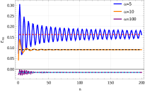
(a)  

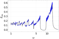
(b)  

Figure 2: (a) The characteristics of residual energy as a function of $n$. The large $n$ saturation value is indicated by the dashed line. The frequencies used are given in the inset. (b) The residual energy at $n=500$ as a function of frequency. The dashed line corresponds to the saturation value given by Eq. (42). The parameters used in this figure are $g_{0}=2$ and $g_{1}=1$.

The saturation value of the residual energy simplifies further for $g_{1}=0$ and $\omega=2\pi$, and is given by

$$E_{res}^{sat}|_{(g_{1}=0)}=\frac{1}{L}\sum_{k>0}\left[(g_{0}-\cos k)n_{kx}^{2}-n_{kx}n_{kz}\sin k\right].$$ (43)

This summation over $k$ values in the Brillouin zone needs to be performed numerically. Additionally, similar expressions for the current operator, given by $\hat{J}=\frac{i}{L}\sum_{i=1}^{L}\left(c_{i}^{\dagger}c_{i+1}-c_{i+1}^{\dagger}c_{i}\right)$, can also be derived. The behavior of the current is similar to that of the residual energy and matches with results found in the literature for different drive protocols[57].

IV Magnetization

In this section, we study the expectation value of the magnetization, defined as the expectation value of $\hat{M}=\sum_{i}\sigma_{i}^{z}$. At stroboscopic intervals, the magnetization is given by

$$M(n)=\frac{2}{L}\sum_{k>0}\left(2|u_{k}(n)|^{2}-1\right).$$ (44)

This quantity is analogous to the density for the Kitaev chain. Following the same calculations as prescribed in the previous section, we obtain the expression for the magnetization after $n$ cycles as

$$M(n) = \frac{2}{L}\sum_{k>0}\left(\Gamma_{k}^{2}(1-\cos 2n\theta_{k})-1\right).$$ (45)

We have plotted the expression for magnetization given by Eq. (45) as a function of $n$ in Fig. 3(a). The initial state from which the evolution starts is $\prod_{k}\left(0,1\right)^{\mathbf{T}}$, which corresponds to the initial magnetization $M(0)=-1$. As discussed in the previous section, at large $n$, the magnetization saturates to a value given by the $n$-independent part of Eq. (45). In Fig. 3(b), we plot the magnetization as a function of drive frequency. For the square pulse protocol, it has been observed that for certain frequencies, the magnetization remains at its initial value and remains almost constant with $n$, leading to a phenomenon known as dynamical freezing. We note that for the periodic kick protocol, this behavior is only present for large values of $g_{0}$. In Fig. 3(b), we use $g_{0}=10$. For large $g_{0}$, $\Gamma_{k}\rightarrow 0$ for all values of $k$, leading to $M=-1$ except at specific frequencies highlighted by the orange vertical lines in Fig. 3(b). This behavior is substantially different from the dynamical freezing reported in the literature. To understand this, we expand $\Gamma_{k}$ for large $g_{0}$. In this limit, the energy dispersion in Eq. (9) can be approximated as $\epsilon_{k}\simeq g_{0}$ and $n_{kz}\simeq 1$. With this approximation, $\Gamma_{k}$ from Eq. (36) simplifies to

$$\Gamma_{k} \simeq \left(\frac{\sin k\sin(Tg_{0})}{g_{0}\sin(g_{1}+Tg_{0})}\right)^{2}.$$ (46)

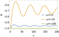
(a)  

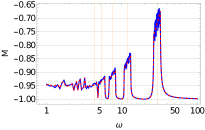
(b)  

Figure 3: (a) The behavior of magnetization as a function of $n$. (b) Magnetization after $n=500$ drive cycles as a function of drive frequency. The dashed line shows the magnetization computed using the large $n$ saturation value from the $n$-independent part of Eq. (45). The parameters used in this figures are $g_{0}=10$, $g_{1}=1$.

For any arbitrary $k$, all $\sin$ terms are less than 1. Moreover, $g_{0}^{2}$ in the denominator makes $\Gamma_{k}$ almost zero for all $k$, except when the $\sin(g_{1}+Tg_{0})$ term in the denominator is close to zero for all $k$. This condition translates to $g_{1}+Tg_{0}=m\pi$, where $m$ is an integer. This gives the frequencies $\omega^{*}=\frac{2g_{0}\pi}{m\pi-g_{1}}$, close to which the freezing phenomenon does not occur. In Fig. 3(b), with $g_{0}=10$ and $g_{1}=1$, we see that close to the frequency $\omega^{*}=\frac{20\pi}{m\pi-1}$, highlighted by the orange vertical line, the magnetization deviates from -1 and can be obtained by using the limiting value of Eq.(46). For higher values of $m$, the vertical lines become very close to each other, resulting in almost flat values of magnetization slightly away from -1. Finally, we can conclude that for the delta kick protocol and high values of $g_{0}$, the magnetization is always dynamically frozen except close to some specific frequencies, which we discuss in detail in this section.

V fidelity

In this section, we present our findings for the fidelity defined as $\chi(n)=\prod_{k}|\langle\psi_{k}(0)|\psi_{k}(nT)\rangle|^{2}$. Using the expression for the wavefunction after the $n$th cycle of the delta kick protocol given by Eq. (13), we calculate the logarithm of the fidelity $g(n)$ as follows:

$$g(n) = \ln\chi(n)=\ln\left(\prod_{k>0}|\langle\psi_{k}(0)|\psi_{k}(nT)\rangle|^{2}\right)$$ (47)

$$= \frac{2}{L}\sum_{k>0}\ln\left(|v_{k}(n)|^{2}\right)=\frac{2}{L}\sum_{k>0}\ln\left(1-|u_{k}(n)|^{2}\right)$$

$$= \frac{2}{L}\sum_{k>0}\ln\left|1-\frac{\Gamma_{k}^{2}}{2}(1-\cos 2n\theta_{k})\right|.$$

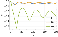
(a)  

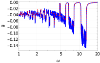
(b)  

Figure 4: (a) Fidelity as a function of $n$. The values of the frequencies are given in the inset. (b) The saturation value of the fidelity after $n=500$ drive cycles plotted as a function of frequency. The dashed line indicates the fidelity computed using the large $n$ saturation value given by Eq. (48). We have used $g_{0}=10$, $g_{1}=1$ in this figure.

We have plotted $g(n)$ as a function of $n$ in Fig. 4(a). Initially, $g(n)$ starts from a certain value, decays, and eventually saturates at a value for large and finite $n$. Note that the highly oscillating term is inside the logarithm, and in this case will contribute to the integral in Eq. (47) even for large but finite $n$. One can show that all the even power terms in the expansion of the logarithm are non-zero. Following the prescription discussed by S. Sharma et al. in Ref. [58], the saturation value is found to be

$$g_{sat} = -\frac{4}{L}\sum_{k>0}\ln\left(\frac{2}{1+\sqrt{1-\Gamma_{k}^{2}}}\right).$$ (48)

In Fig. 4(b), we plot $g(500)$ as a function of frequency. The dashed line indicates the $g(n\to\infty)$ value given by Eq. (48). We observe that $g(500)$ oscillates around the $g(n\to\infty)$ value, and for particular frequencies where $\Gamma_{k}=0$, $g(n)$ approaches 1, similar to the behavior of magnetization discussed earlier.

VI Correlation function

In this section, we use the analytical expression for $|\psi(nT)\rangle$ given in Eq. (31) to explore the dynamical relaxation behavior of our system under delta-kick driving. We first calculate two nontrivial fermionic correlators to study the dynamical relaxation behaviour of the system[59, 60, 61, 62, 63]. The fermionic correlators are defined as:

$$C_{ij}(t) = \frac{2}{L}\sum_{k>0}|u_{k}(t)|^{2}\cos(k(i-j)),$$ (49)

$$F_{ij}(t) = \frac{2}{L}\sum_{k>0}u_{k}^{*}(t)v_{k}(t)\sin(k(i-j)).$$ (50)

Understanding the behavior of the correlation functions are crucial as it contains the information about quantum criticality. Recent studies have identified that singularities in certain out-of-time-ordered correlation functions for finite-length products indicate the presence of dynamical phase transitions[64]. Using Wick’s theorem, all correlation functions of the system can be expressed through these two nontrivial correlations. As a result, we proceed to determine the $C$ and $F$ matrices stroboscopically. It is evident from the definitions that for $i=j$, the diagonal terms of the $C$ matrix are all equal, whereas the diagonal terms of the $F$ matrix are all zero. Using the fact that the elements of the $C$ and $F$ matrices depend only on $i-j$, we define an integer variable $m=i-j$ and obtain the analytical expression for all the non-zero terms of the $C$ matrix:

$$C_{m}(n) = \frac{1}{L}\sum_{k>0}\Gamma_{k}^{2}\cos(mk)(1-\cos 2n\theta_{k}).$$ (51)

The $F$ matrix is complex, and following a similar prescription, we also obtain the analytical expression for the $F$ matrix:

$$F_{m}^{R}(n) = -\frac{1}{L}\sum_{k>0}\frac{\Gamma_{k}\sin mk}{\sin\theta_{k}}(\sin g_{1}\cos\Phi_{k}$$ (52)

$$+n_{kz}\cos g_{1}\sin\Phi_{k})(1-\cos 2n\theta_{k}),$$

$$F_{m}^{I}(n) = \frac{1}{L}\sum_{k>0}\Gamma_{k}\sin mk\sin 2n\theta_{k}.$$ (53)

Here $F_{m}^{R}$ and $F_{m}^{I}$ are the real and imaginary parts of the complex $F$ matrix, respectively. From Eqs. (51, 52, 53), it is clear that the terms independent of $n$ survive in the limit of large but finite $n$, leading to convergence to a generalized Gibbs ensemble (GGE)[65, 66]. At large $n$, the imaginary part of the $F$ matrix vanishes, and both $C$ and $F$ matrices become real. This can be explained by the fact that the system absorbs energy from the periodic drive and heats up to a steady state characterized by the conserved quantities of the integrable system. We have plotted the correlation functions as a function of $n$ in Fig.5(a) for $m=2$.

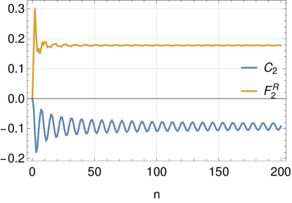
(a)  

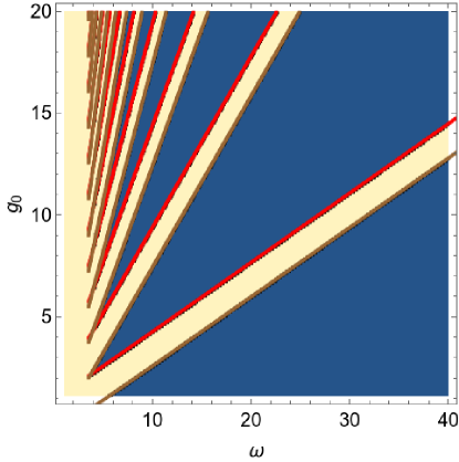
(b)  

Figure 5: (a) Correlation function $C_{2}$ and $F_{2}^{R}$ is plotted as a function of $n$ using Eq.(51, 52). (b)The phase diagram of dynamical transition in relaxation behaviour. Blue region signify relaxation with power law $-\frac{3}{2}$ while the yellow region has powerlaw $-\frac{1}{2}$. At the transition point red and brown lines (the solution of Eq.(54)) the powerlaw of the relaxation behaviour is $-\frac{3}{4}$. Here we have taken $g_{1}=1$.

Next, we study the approach to the steady state. We have plotted in Fig. (6) the $n$-dependent part of the correlation matrix, $\delta C_{m}(n)=\frac{1}{L}\sum_{k>0}\Gamma_{k}^{2}\cos(mk)(\cos 2n\theta_{k})$, which decays following a power law as reported in earlier literature. This power law behavior arises from both slowly varying and highly oscillating terms and universal in all local observable. Using the saddle-point approximation discussed in Ref. [59], one can approximate the $n$-dependent part of the correlation function at large $n$. Since the $n$-dependent part is highly oscillatory, most of the contribution to the integral in Eqs. (51, 52, 53) comes from the saddle point at $k=k_{0}$, where $\theta_{k}$ is at an extremum. The value of $k_{0}$ can be calculated by differentiating Eq. (34) with respect to $k$ and equating it to zero. Although an analytical expression for the first derivative of $\theta_{k}$ is possible, solving the resulting transcendental equation numerically yields the value of $k_{0}$. In the delta-kick protocol, the extremum of $\theta_{k}$ usually occurs at $k_{0}=0$ or $\pi$, and at these points, $\Gamma_{k}=0$ due to the presence of $\sin k$ in the numerator from $n_{kx}$. This causes the slowly varying term to vanish at $k=k_{0}$, leading to a power law behavior characterized by an exponent of $-3/2$. Conversely, for some values of $\omega$, the saddle point occurs at $k_{0}\neq 0$ or $\pi$, where the slowly varying term is non-zero, resulting in a power law behavior characterized by an exponent of $-1/2$. A dynamical transition between these two power law behaviors occurs as a function of drive frequency, with the critical frequency $\omega_{c}$ defining the transition. In Fig. (5(a)), we reproduce the phase diagram of this dynamical transition, first reported in Ref. [59]. In the blue region of the phase diagram, the roots of $\frac{d\theta_{k}}{dk}=0$ are only $0$ and $\pi$, indicating a $-3/2$ relaxation behavior. In the yellow region, other roots of the equation $\frac{d\theta_{k}}{dk}=0$ are possible, leading to a $-1/2$ relaxation behavior. At the transition from the blue to the yellow region, an extra root appears in the equation $\frac{d\theta_{k}}{dk}=0$, implying that $\frac{d^{2}\theta_{k}}{dk^{2}}=0$ exactly at the transition point. This gives the critical frequency $\omega_{c}$ where the transition occurs, defined by the solution to the equation:

$$\tan\left(\frac{z_{\pm}}{\omega}\right)=\mp\frac{\left(\frac{z_{\pm}g_{0}}{\omega}\right)\tan g_{1}}{\tan g_{1}\pm\left(\frac{z_{\pm}g_{0}}{\omega}\right)},$$ (54)

where $z_{\pm}=2\pi(g_{0}\pm 1)$. The $+$ and $-$ signs correspond to $k_{0}=\pi$ and $0$, respectively, reflecting the fact that the extra root of the equation $\frac{d\theta_{k}}{dk}=0$ arises either from the $0$ or $\pi$ side. We numerically solve Eq. (54) and plot it in Fig. (5(a)). The red and brown lines correspond to the solutions for the $+$ and $-$ signs of the equation, respectively. This Eq.(54) is a new result and matches with Ref. [59].

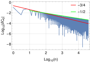
(a)  

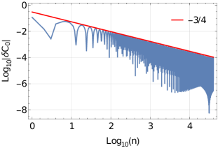
(b)  

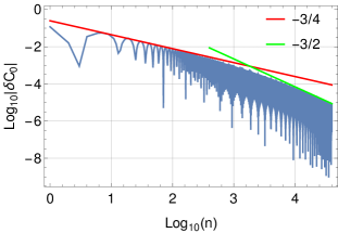
(c)  

Figure 6: We have plotted $\log|\delta C_{0}(n)|$ as a function of $\log n$. (a) $\omega=8.24094$, slightly below the critical frequency. (b) $\omega_{c}=8.26094$, at the critical frequency. (c) $\omega=8.28094$, slightly above the critical frequency. The red and green lines are guides to the eye. Here we have taken $g_{0}=2$, $g_{1}=1$ and system size $L=80000$.

Recently, it has been observed in [61] that at the dynamical transition point, the relaxation behavior of the $n$-dependent part of the correlators shows a different power law behavior characterized by an exponent of $-3/4$. At this transition point, not only are the first and second derivatives of $\theta_{k}$ zero, but the third derivative is also zero. The first non-zero term in the Taylor series expansion of $\theta_{k}$ is of fourth order. Moreover, on the transition line, $k_{0}=0$ or $\pi$, which corresponds to $\Gamma_{k}=0$. Therefore, we must modify the saddle-point approximation defined in Ref. [59] by including higher-order terms. The modified approximation is given by[67, 68]:

$$\int dk\,f(k)e^{in\theta_{k}}\simeq e^{-in\theta_{k_{0}}}e^{i\frac{7\pi}{8}}\frac{6f^{\prime\prime}(k_{0})\Gamma\left(\frac{3}{4}\right)}{(24)^{\frac{1}{4}}(|\theta_{k_{0}}^{\prime\prime\prime\prime}|)^{\frac{3}{4}}}n^{-\frac{3}{4}},$$ (55)

where $f(k)$ is the slowly varying part of the correlators that contains $\Gamma_{k}$, $f(k_{0})=0$ and $f^{\prime}(k_{0})=0$. The $n^{-\frac{3}{4}}$ term clearly explains the critical relaxation behavior. In Fig. (6), we have plotted $|\delta C_{0}(n)|$ as a function of $n$ for three different frequencies. Fig. (6(a)) shows the relaxation behavior below the critical frequency but very close to it. Due to this, the initial relaxation follows a power law with an exponent of $-3/4$, but at large $n$, a transition to an exponent of $-1/2$ is observed. Fig. (6(b)) shows critical relaxation characterized by the exponent $-3/4$. Fig. (6(c)) shows dynamical relaxation above the critical frequency but very close to it, where a transition from $-3/4$ to $-3/2$ is visible. Using the saddle-point approximation at the critical point, we find a simplified numerical expression for $|\delta C_{0}(n)|$ that demonstrates the power law scaling:

$$|\delta C_{0}(n)|\simeq 1.79067\frac{\cos(3.00142n)}{n^{\frac{3}{4}}}.$$ (56)

Similar expressions for $\delta F_{m}^{R}(n)$ and $\delta F_{m}^{I}(n)$ can also be derived and are straightforward to calculate.
Using the analytical expressions for the $C$ and $F$ matrices given by Eqs. (51, 52, 53), we compute the correlator matrix $\Pi$ defined as:

$$\Pi_{n}(l)=\left(\begin{array}[]{cc}{\mathbb{I}}_{l}-C&F\\ F^{*}&C\end{array}\right),$$ (59)

where $l$ is the subsystem size and the indices $i,j$ of the $C$ and $F$ matrices are restricted to within the subsystem. The entanglement entropy[69, 70, 71, 72] is given by $S_{n}(l)=-\sum_{i}\rho_{i}\ln\rho_{i}$, where $\rho_{i}$ are the eigenvalues of the $\Pi_{n}(l)$ matrix. We have numerically diagonalized the correlator matrix to compute the entanglement entropy, which is plotted in Fig. (7). Our analytical expressions simplify the calculation, as numerical computation of the $n$-th power of the evolution matrix is not required. In Fig. (7(a)), we plot the entanglement entropy as a function of $n$. It starts from zero since the initial state is a product state and saturates to a value proportional to the length[73] of the subsystem at large $n$. Fig. (7(b)) shows the behavior of the entanglement entropy as a function of drive frequency after $n=200$ drive cycles. At large drive frequencies, the system fails to respond to the external periodic drive, and the system remains in the initial product state, resulting in the entanglement entropy remaining at zero even after many drive cycles.

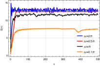
(a)  

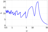
(b)  

Figure 7: (a) The behavior of entanglement entropy as a function of drive cycle $n$. The values of the frequencies are given in the inset. (b) The saturation value of entanglement entropy after $n=200$ drive cycles as a function of drive frequency. Here $g_{0}=2$, $g_{1}=1$, $L=1000$ and $l=50$.

VII Discussion

In this paper, we have studied periodically driven integrable systems, focusing specifically on the long-time dynamics of a periodically delta-kicked transverse field Ising model. We derive an analytical expression for the time-evolution operator over one period and use this to obtain the exact analytical expression for the time-dependent state at stroboscopic intervals. This time-dependent wave function enables the calculation of the expectation value of any observable after the $n$-th drive cycle. Initially, we derive the expression for the defect density, which consists of two components: a highly oscillatory part that varies with $\theta_{k}$, the eigenvalue of the evolution operator over one period. The number of oscillations in exciatation probablity for each $k$ increases with drive cycle $n$. The second term in $n_{d}$ is independent of $n$, representing the periodic-GGE and providing the saturation value for large $n$. This feature is universal across the expectation values of all observables. Next, we compute the expectation values of residual energy, magnetization, and fidelity. For large values of $\mu_{0}$, the magnetization exhibits dynamic freezing for almost all drive frequencies, except for a few specific frequencies where it deviates from its initial value. These frequencies, given by $\omega^{*}=\frac{2g_{0}\pi}{m\pi-g_{1}}$, are analyzed for their significance. The residual energy and fidelity show similar behavior at these frequencies. We then derive the analytical expressions for all elements of the correlation matrix after the $n$-th drive cycle and discuss the relaxation behavior of the correlators, which is true for all observables. Depending on the drive frequency, the relaxation behavior changes the slope of the approach to the steady state from $-3/2$ to $-1/2$. This represents a rare example of a dynamical transition and the emergence of universality in driven systems. At the transition point, the critical relaxation is characterized by a slope of $-3/4$. We derive equations for the critical frequencies, assuming $g_{0}$ and $g_{1}$ are fixed, and solve these equations numerically, finding the values of critical frequencies which matches with those reported in the literature. Finally, we numerically compute the entanglement entropy (EE) using the analytical expressions for the correlation matrix and discuss its properties. Our results for EE are consistent with earlier numerical findings obtained using Floquet theory.
In conclusion, we have explored the long-time dynamics of a periodically driven integrable system in one dimension. Exact analytical expressions for the stroboscopic time-dependent wave function after the $n$-th drive period have been derived and used this to calculate the expectation values of defect density, residual energy, magnetization, fidelity, and two non-trivial quadratic correlators. We have discussed their properties based on these analytical expressions and derived an expression for the dynamical phase boundary that separates different relaxation behaviors of the observables. Our work opens several avenues for future research, including investigating analytical solutions for other periodic driving protocols and extending the current study to integrable long-range[74] and non-Hermitian systems[75, 76, 77, 78].

VIII Acknowledgments

The authors thank Prof. Diptiman Sen and Prof. Bhabani Prasad Mandal for numerous discussions on related topics. A.D. acknowledges financial support from the SERB-SRG grant SRG/2022/001145 and the IoE seed grant from BHU IoE/Seed Grant II/2021-22/39963.

IX Appendix

In this section, we outline the procedure to derive the expression for the $n$th power of the evolution matrix over one period. We extend the calculation developted for a locally periodic system by D. J. Griffiths et al. [49] to a periodically driven system. We start with the characteristic equation of $U_{k}(T)$, given by $\det(U_{k}(T)-\lambda\mathbb{I}_{2\times 2})=0$, where $\lambda$ represents the eigenvalues of the unitary matrix. Assuming $\xi_{k}=\frac{1}{2}\operatorname{Tr}(U_{k}(T))$, we can rewrite the characteristic equation as

$$\lambda^{2}-2\lambda\xi_{k}+1=0.$$ (60)

Here, we use the fact that $\det(U_{k}(T))=1$. Applying the Cayley-Hamilton theorem, we obtain

$$U_{k}^{2}(T)-2\xi_{k}U_{k}(T)+\mathbb{I}_{2\times 2}=0.$$ (61)

This equation shows that all higher power of $U_{k}(T)$ can be expressed as a linear combination of $U_{k}(T)$ and the identity matrix. We assume:

$$U_{k}^{n}(T)=\mathcal{F}_{n-1}(\xi_{k})U_{k}(T)+\mathcal{F}_{n-2}(\xi_{k})\mathbb{I}_{2\times 2},$$ (62)

where the coefficients $\mathcal{F}_{n-1}(\xi_{k})$ represents polynomials of degree $n-1$ in $\xi_{k}$, yet to be determined. Using the method of induction, one can straightforwardly derive the recurrence relation for these polynomials, which turns out to be consistent with the recurrence relation of the Chebyshev polynomials of second kind.

References

- [1] Jacek Dziarmaga, Adv. Phys. 59, 1063 (2010).
- [2] A. Polkovnikov, K. Sengupta, A. Silva, and M. Vengalattore, Rev. Mod. Phys. 83, 863 (2011).
- [3] M. Bukov, L. D’Alessio and A. Polkovnikov, Advances in Physics 64, 139 (2015);
- [4] L. D’Alessio, Y. Kafri, A. Polkovnikov, and M. Rigol, Adv. Phys. 65, 239 (2016).
- [5] A. Dutta, G. Aeppli, B. K. Chakrabarti, U. Divakaran, T. F. Rosenbaum, and D. Sen, Quantum phase transitions in transverse field spin models: from statistical physics to quantum information (Cambridge University Press, 2015).
- [6] Quantum Integrability in out of Equilibrium Systems, edited by P. Calabrese, F. H. L. Essler, and G. Mussardo, special issue of J. Stat. Mech. (IOP Science, 2016), pp. 064001–064011.
- [7] Tomotaka Kuwahara, Takashi Mori, Keiji Saito, Annals of Physics, 367, 96–124, (2016).
- [8] J. I. Cirac and P. Zoller, Nature Phys. 8, 264(2012).
- [9] M. Greiner, O. Mandel, T. Esslinger, T. W. Hansch, and I. Bloch, Nature 39, 415 (2002).
- [10] J. Simon, W. S. Bakr, R. Ma, M. E. Tai, P. M. Preiss, and M. Greiner, Nature (London) 472, 307 (2011)
- [11] W. Bakr, A. Peng, E. Tai, R. Ma, J. Simon, J. Gillen, S. Foelling, L. Pollet, and M. Greiner, Science 329, 547 (2010).
- [12] H. Bernien, S. Schwartz, A. Keesling, H. Levine, A. Omran, H. Pichler, S. Choi, A. S. Zibrov, M. Endres, M. Greiner, V. Vuletic, and M. D. Lukin, Nature 551, 579 (2017).
- [13] Rajibul Islam, Ruichao Ma, Philipp M. Preiss, M. Eric Tai, Alexander Lukin, Matthew Rispoli and Markus Greiner, Nature, 528, pages77–83 (2015).
- [14] Arnab Sen, Diptiman Sen and K Sengupta, J. Phys.: Condens. Matter 33 (2021) 443003.
- [15] Angelo Russomanno, Giuseppe E Santoro and Rosario Fazio, 7, (2016) 073101.
- [16] André Eckardt and Egidijus Anisimovas, New J. Phys. 17, 093039, (2015).
- [17] Vladimir Gritsev and Anatoli Polkovnikov, SciPost Phys. 2, 021, (2017).
- [18] Yang Song, J. P. Kestner, Xin Wang, and S. Das Sarma, Phys. Rev. A 94, 012321 (2016).
- [19] Denis Gagnon, François Fillion-Gourdeau, Joey Dumont, Catherine Lefebvre, and Steve MacLean, Phys.Rev.Lett. 119, 053203 (2017).
- [20] S. K. Earl, M. A. Conway, J. B. Muir, M. Wurdack, E. A. Ostrovskaya, J. O. Tollerud, and J. A. Davis, Phys. Rev. B 104, L060303, (2021).
- [21] Matteo Lucchini, Fabio Medeghini, Yingxuan Wu, Federico Vismarra, Rocío Borrego-Varillas, Aurora Crego, Fabio Frassetto, Luca Poletto, Shunsuke A. Sato, Hannes Hübener, Umberto De Giovannini, Ángel Rubio and Mauro Nisoli, Nat. Commun. 13, 7103 (2022).
- [22] Michael Messer, Kilian Sandholzer, Frederik Görg, Joaquín Minguzzi, Remi Desbuquois, and Tilman Esslinger, Phys. Rev. Lett. 121, 233603,(2018).
- [23] K. Ono, S. N. Shevcheko, T. Mori, S. Moriyama and Franco Nori, Phys. Rev. Lett. 125, 166802, (2020).
- [24] T. Nag, S. Roy, A. Dutta, and D. Sen, Phys. Rev. B 89, 165425 (2014); T. Nag, D. Sen, and A. Dutta, Phys. Rev. A 91, 063607(2015).
- [25] A. Agarwala, U. Bhattacharya, A. Dutta, and D. Sen, Phys. Rev. B 93, 174301 (2016); A. Agarwala and D. Sen, Phys. Rev. B 95, 014305 (2017).
- [26] D. J. Luitz, Y. Bar Lev, and A. Lazarides, SciPost Phys. 3, 029 (2017); D. J. Luitz, A. Lazarides, and Y. Bar Lev, Phys. Rev. B 97, 020303 (2018).
- [27] A. Das, Phys.Rev. B 82, 172402, (2010).
- [28] S Bhattacharyya, A Das, and S Dasgupta, Phys. Rev. B 86, 054410, (2010).
- [29] S. Hegde,H. Katiyar, T. S. Mahesh, and A. Das, Phys. Rev. B 90, 174407, (2014)
- [30] S. Mondal, D. Pekker, and K. Sengupta, Europhys. Lett. 100, 60007 (2012).
- [31] U. Divakaran and K. Sengupta, Phys. Rev. B 90, 184303 (2014).
- [32] Oleh V. Ivakhnenko, Sergey N. Shevchenko and Franco Nori, Physics Reports 995, (2023).
- [33] M. Heyl, A. Polkovnikov, and S. Kehrein, Phys. Rev. Lett. 110, 135704 (2013); For a review, see M. Heyl, Rep. Prog. Phys 81, 054001 (2018).
- [34] T. Oka and H. Aoki, Phys. Rev. B 79, 081406 (R) (2009).
- [35] T. Kitagawa, E. Berg, M. Rudner, and E. Demler, Phys. Rev. B 82, 235114 (2010); N. H. Lindner, G. Refael, and V. Galitski, Nat. Phys. 7, 490 (2011).
- [36] T. Kitagawa, T. Oka, A. Brataas, L. Fu, and E. Demler, Phys. Rev. B 84, 235108 (2011); B. Mukherjee, P. Mohan, D. Sen, and K. Sengupta, Phys. Rev. B 97, 205415 (2018).
- [37] F. Nathan and M. S. Rudner, New J. Phys. 17, 125014 (2015);
- [38] M. S. Rudner, N. H. Lindner, E. Berg, and M. Levin, Phys. Rev. X 3, 031005 (2013).
- [39] Ranjani Seshadri, Anirban Dutta and Diptiman Sen, Phys. Rev. B 100, 115403 (2019).
- [40] Bhaskar Mukherjee, Arnab Sen, Diptiman Sen and K. Sengupta, Phys. Rev. B 102, 014301 (2020).
- [41] B. Mukherjee, S. Nandy, A. Sen, D. Sen and K. Sengupta, Phys. Rev B 101, 245107 (2020)
- [42] B. Mukherjee, A. Sen, D. Sen and K. Sengupta, Phys. Rev B 102, 075123 (2020).
- [43] B. Mukherjee, A. Sen, and K. Sengupta, Phys. Rev. B 106, 064305 (2022).
- [44] S. Ghosh, I. Paul, and K. Sengupta, Phys. Rev. Lett. 130, 120401 (2023).
- [45] Nobuyuki Okuma, and Masatoshi Sato, Annu. Rev. Condens. Matter Phys.,14, 83–107 (2023).
- [46] S. Sachdev, Quantum Phase Transitions(Cambridge University Press, Cambridge, England, 1999).
- [47] Manisha Thakurathi, Aavishkar A. Patel, Diptiman Sen and Amit Dutta, Phys. Rev. B 88, 155133 (2013).
- [48] Saikat Mondal, Diptiman Sen and Amit Dutta, J. Phys.: Condens. Matter , 35 085601.
- [49] D. J. Griffiths and C. A. Steinke, Am. J. Phys. 69, 137–154 (2001).
- [50] Zhi-Cheng Shi, Ye-Hong Chen, Wei Qin,Yan Xia, X.X.Yi, Shi-Biao Zheng, and Franco Nori, Phys. Rev. A 104, 053101 (2021).
- [51] T. W. B. Kibble, J. Phys. A: Math. Gen. 9, 1387 (1976); Phys. Rep. 67, 183 (1980).
- [52] W. H. Zurek, Nature (London) 317, 505 (1985); Acta Phys. Pol. B 24, 1301 (1993); Phys. Rep. 276, 177 (1996).
- [53] Anirban Dutta, C. Trefzger and K. Sengupta, Phys. Rev. B 86, 085140 (2012).
- [54] Anirban Dutta, Armin Rahmani and Adolfo del Campo, Phys. Rev. Lett. 117, 080402 (2016).
- [55] Angelo Russomanno and Emanuele G. Dalla Torre, EPL 115 30006 (2016).
- [56] Anirban Dutta, Arnab Das and K Sengupta, Phys. Rev. E 92, 012104 (2015).
- [57] Somnath Maity, Utso Bhattacharya and Amit Dutta, Phys. Rev. B 98], 064305 (2018).
- [58] Shraddha Sharma, Angelo Russomanno, Giuseppe E. Santoro and Amit Dutta, EPL 106 67003.
- [59] Arnab Sen, Sourav Nandy and K. Sengupta, Phys. Rev. B 94, 214301 (2016).
- [60] Sourav Nandy, Arnab Sen and Diptiman Sen, Phys. Rev. X 7, 031034 (2017).
- [61] Sreemayee Aditya, Sutapa Samanta, Arnab Sen, K. Sengupta and Diptiman Sen, Phys. Rev. B 105, 104303 (2022).
- [62] Aamir Ahmad Makki, Souvik Bandyopadhyay, Somnath Maity and Amit Dutta, Phys. Rev. B 105, 054301 (2022).
- [63] Madhumita Sarkar and K. Sengupta, Phys. Rev. B 107, 235154 (2020).
- [64] S. Bandyopadhyay, A. Polkovnikov, and A. Dutta,Phys. Rev. Lett. 109, 094306 (2024).
- [65] Achilleas Lazarides, Arnab Das and Roderich Moessner, Phys. Rev. Lett. 112, 150401 (2014).
- [66] Sourav Nandy, Arnab Sen, Arnab Das and Abhishek Dhar, Phys. Rev. B 94, 245131 (2016).
- [67] Carl M. Bender and Steven A.Orszag, Advanced Mathematical Methods for Scientists and Engineers, Asymptotic Methods and Perturbation Theory (1999).
- [68] N. Bleistein and R A.Handelsman,Asymptotic Expansions of Integrals (2010).
- [69] G.Vidal, J.I.Latorre, E.Rico and A.Kitaev, Phys. Rev. Lett. 90, 227902 (2003).
- [70] J. Eisert, M. Cramer, and M. B. Plenio, Rev. Mod. Phys. 82, 277 (2010).
- [71] L. Amico, R. Fazio, A. Osterloh, and V. Vedral, Rev. Mod. Phys. 80, 517 (2008).
- [72] P. Calabrese and J. Cardy, J. Stat. Mech. 6, 06002 (2004); R.Ghosh, N. Dupuis, A. Sen, and K. Sengupta, Phys. Rev. B 101, 245130 (2020).
- [73] M. B. Hastings, J. Stat. Mech., 8, P08024 (2007).
- [74] Anirban Dutta and Amit Dutta, Phys. Rev. B 96, 125113 (2017).
- [75] Tista Banerjee and K. Sengupta, Phys. Rev. B 107, 155117 (2023).
- [76] Tista Banerjee and K. Sengupta, arXiv:2407.20764, (2024).
- [77] Tista Banerjee and K.Sengupta, Phys. Rev. B. 109, 094306 (2024).
- [78] J-J Liu, Z-W. Li, Z-G. Chen, W. Tang, A. Chen, B. Liang, G. Ma, and J-C. Cheng Phys. Rev. Lett. 129, 084301 (2022).