Thermal leptogenesis, dark matter and gravitational waves from an extended canonical seesaw

Abstract

In a canonical type-I seesaw scenario, the SM is extended with three singlet right-handed neutrinos (RHNs) $N_{i},i=1,2,3$ with masses $M_{i},i=1,2,3$ to simultaneously explain sub-eV masses of light neutrinos and baryon asymmetry of the Universe. In this paper, we show that a relatively low-scale thermal leptogenesis accompanied by gravitational wave signatures is possible when the type-I seesaw is extended with a singlet fermion ($S$) and a singlet scalar ($\rho$), where $S$ and $\rho$ are odd under a discrete $Z_{2}$ symmetry. We also add a vector-like fermion doublet $\Psi$ and impose a $Z^{\prime}_{2}$ symmetry under which both $N_{1}$ and $\Psi$ are odd while all other particles are even. This gives rise to a singlet-doublet Majorana fermion dark matter in our setup. At a high scale, the $Z_{2}$ symmetry is broken spontaneously by the vacuum expectation value of $\rho$ and leads to : (i) mixing between RHNs ($N_{2},N_{3}$) and S, and (ii) formation of Domain walls (DWs). In the former case, the final lepton asymmetry is generated by the out-of-equilibrium decay of $S$, which dominantly mixes with $N_{2}$. We show that the scale of thermal leptogenesis can be lowered to $M_{S}\sim 4\times 10^{8}$ GeV. In the latter case, the disappearance of the DWs gives observable gravitational wave signatures, which can be probed at NANOGrav, EPTA, LISA, etc.

I Introduction

Recently NANOGrav[1, 2], EPTA [3], PPTA [4] have reported positive evidence for stochastic gravitational wave (GW) background in the nanohertz (nHz) frequency range. This stochastic GW background could originate from various sources. One such possibility is the domain walls (DWs) which are two-dimensional topological defects that emerge when a discrete symmetry is spontaneously broken in the early universe [5]. In cosmology, the formation of DWs possess a significant challenge because their energy density can quickly surpass the total energy density of the Universe, which contradicts current observational data [6]. However, it’s possible that DWs are inherently unstable and collapse before they can dominate the total energy density of the Universe. This instability could be due to an explicit breaking of the discrete symmetry in the underlying theory [7, 8, 9]. If this is the case, a considerable amount of GWs could be generated during the collisions and annihilations of these domain walls [10, 11, 12, 13, 14, 15, 16]. These GWs might persist as a stochastic background in the universe today. Detecting these GWs would offer insights into early cosmic events and provide a novel method for exploring physics at extremely high energies.

In this paper, we try to connect the non-zero neutrino mass, dark matter (DM), observed baryon asymmetry of the Universe and the GW sourced by the DWs in a common framework as shown pictorially in Fig 1. With this motivation, we extend the canonical type-I seesaw model[17, 18, 19] with a singlet fermion: $S$ and one singlet scalar: $\rho$. We impose a discrete $Z_{2}$ symmetry under which $S$ and $\rho$ are odd while all other particles are even. This forbids the direct coupling of $S$ with the $L,H$. We also introduce a vector-like fermion doublet $\Psi\equiv\left(\psi^{0}~{}\psi^{-}\right)^{T}$ and impose a discrete symmetry $Z^{\prime}_{2}$ under which $\Psi$ and the lightest RHN ($N_{1}$) are odd while all other particles are even.

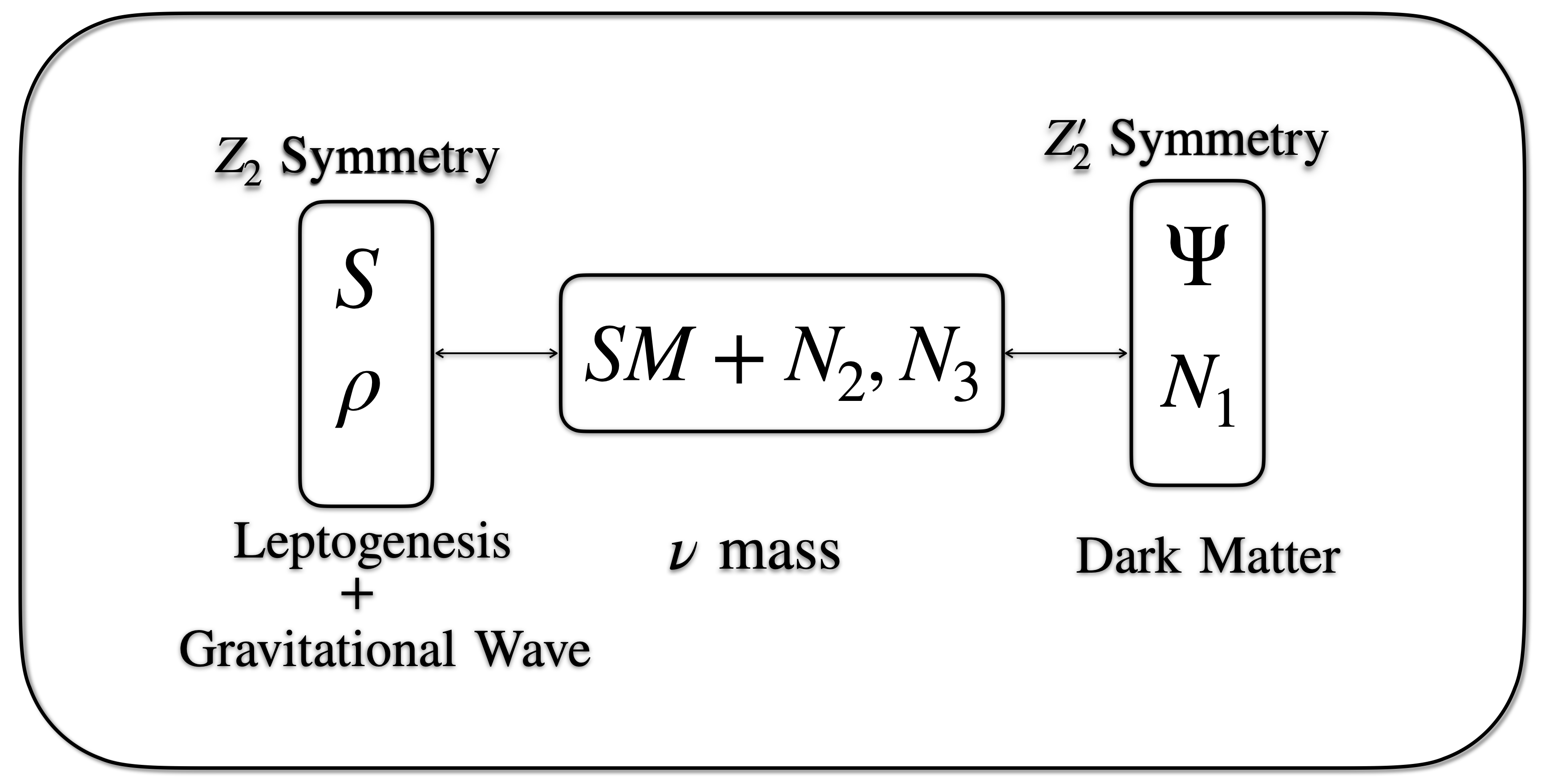
Figure 1: The schematic picture of our setup.

This gives rise a singlet-doublet Majorana fermion DM [20, 21, 22, 23, 24, 25, 26, 27, 28, 29, 30, 31, 32, 33, 34, 35, 36, 37, 38, 39, 40, 41, 42]. At a high scale, when the singlet scalar $\rho$ obtains a vacuum expectation value (vev), the $Z_{2}$ symmetry gets broken and leads to : (i) mixing between the singlet fermion $S$ and RHNs ($N_{2},N_{3}$), (ii) formation of Domain walls (DWs) [6, 43, 7, 44, 45, 46]. In the former case, the $S$ decays to the SM lepton, $L$ and $H$ via the mixing with $N_{2,3}$. Assuming a hierarchy among the $S$ and $N_{2,3}$, the final lepton asymmetry is established by the CP violating out-of-equilibrium decay of $S$. Due to the mixing, the decay width of $S\rightarrow LH$ will be suppressed compared to the usual type-I case $N\rightarrow LH$. As a result the out-of-equilibrium condition can be satisfied for lower values of the mass of $S$. The CP asymmetry parameter does not have any suppression. It depends on the value of $M_{S}$ unlike $M_{N}$ in the usual case. However the value of $M_{S}$ can not be arbitrarily small since it will make the CP asymmetry parameter $\epsilon_{S}$ very small. We find that the leptogenesis scale can be brought down to $\mathcal{O}(10^{8})$ GeV, which is one orders of magnitude smaller than the canonical type-I leptogenesis. We then study the dynamics of the DWs generated by the spontaneous breaking of $Z_{2}$ symmetry. We make them unstable by introducing an explicit $Z_{2}$ breaking term in the scalar potential which creates a pressure difference across the wall. As a result the DWs collapse and annihilate. Stochastic GWs get produced as an out come this explicit breaking of $Z_{2}$. It has to be noted that it is the vev of $\rho$ which connects the leptogenesis and the GW in our framework. We show the parameter space satisfying leptogenesis and GW simultaneously.

The paper is organized as follows. We discuss the model in Section II. In Section III we discuss a low energy thermal leptogenesis scenario arising from a $Z_{2}$ symmetry breaking. The domain wall dynamics and signature of gravitational waves are discussed in Section IV. The DM phenomenology is discussed in Section V. We finally conclude in Section VI.

II The model

We extend the SM with three RHNs, $N_{i},i=1,2,3$ with masses $M_{i},i=1,2,3$, one singlet fermion $S$ with mass $M_{S}$ and one singlet scalar $\rho$.

Table 1: Particles and their charge assignment under the imposed symmetry.

Field	$SU(3)_{c}$	$SU(2)_{L}$	$U(1)_{Y}$	$Z_{2}$	$Z_{2}^{\prime}$
$N_{1}$	1	1	0	+	–
$N_{2,3}$	1	1	0	+	+
$S$	1	1	0	–	+
$\rho$	1	1	0	–	+
$\Psi$	1	2	–1	+	–

We impose a discrete symmetry $Z_{2}$ under which $S$ and $\rho$ are odd, while all other particles are even. As a result the direct coupling of $S$ with $L,H$ is forbidden. We also introduce a vector-like fermion doublet $\Psi\equiv\left(\psi^{0}\psi^{-}\right)^{T}$ and impose an additional discrete symmetry $Z^{\prime}_{2}$ under which $\Psi$ and $N_{1}$ are odd, while all other particles are even. The neutral component of $\Psi^{0}$ combines with $N_{1}$ to give rise a singlet-doublet fermion dark matter. The relevant Lagrangian involving $N$, $S$ and $\rho$ is given as,

$$\mathcal{L} = \bar{N}i\gamma_{\mu}\partial^{\mu}N+\bar{S}i\gamma_{\mu}\partial^{\mu}S-y_{{}_{Nl}}\bar{L}\tilde{H}N-y_{{}_{NS}}\bar{N}\rho S$$ (1)

$$- \frac{1}{2}M_{S}\bar{S^{c}}S-\frac{1}{2}M_{N}\bar{N^{c}}N+h.c,$$

where $N$ denotes $N_{2},N_{3}$.

The scalar potential involving the SM Higgs doublet $H$ and singlet scalar $\rho$ can be written as

$$V(H,\rho) = -\mu_{H}^{2}H^{\dagger}H-\mu^{2}_{\rho}\rho^{2}+\lambda_{H}(H^{\dagger}H)^{2}+\lambda_{\rho}\rho^{4}$$ (2)

$$+ \lambda_{H\rho}(H^{\dagger}H)\rho^{2}.$$

Here we chose $\mu_{\rho}^{2},\mu_{H}^{2}>0$. At a temperature much above the electroweak scale $\rho$ acquires a vev $v_{\rho}$ and breaks the discrete $Z_{2}$ symmetry spontaneously. Similarly the electroweak symmetry breaking (EWSB) occurs when the SM Higgs obtains a vev $v_{h}$. The vacuum fluctuations of the scalar fields are given as

$$H=\frac{1}{\sqrt{2}}(0,h+v_{h})^{T},~{}~{}\rho=\frac{\rho^{\prime}+v_{\rho}}{\sqrt{2}},$$ (3)

where $v_{h}^{2}=\frac{2\mu_{H}^{2}-\lambda_{H\rho}v_{\rho}^{2}}{2\lambda_{H}}$, and $v_{\rho}^{2}=\frac{2\mu_{\rho}^{2}-\lambda_{H\rho}v_{h}^{2}}{2\lambda_{\rho}}$.

II.1 Neutrino mass

Above electroweak phase transition (EWPT), the singlet scalar $\rho$ acquires a vev: $v_{\rho}$ and breaks the $Z_{2}$ symmetry spontaneously. This allows the singlet fermion $S$ to mix with the RHNs $N_{2}$ and $N_{3}$. In the effective theory, the $6\times 6$ fermion mass matrix can be written in the basis $[L_{i},N_{2,3},S]$ as

$$\mathcal{M}=\begin{pmatrix}0&m_{D}&0\\ m_{D}&M_{N}&d\\ 0&d&M_{S}\end{pmatrix},$$ (4)

where $d=y_{{}_{NS}}v_{\rho}/\sqrt{2}$, $m_{D}=y_{{}_{Nl}}v_{h}/\sqrt{2}$.

Now Diagonalising this mass matrix we obtain the masses of heavy eigenstates as

$$M_{N}^{\prime}\simeq M_{N}+\frac{d^{2}}{M_{N}-M_{S}},$$ (5)

$$M_{S}^{\prime}\simeq M_{S}-\frac{d^{2}}{M_{N}-M_{S}},$$ (6)

where the mixing angle is given as

$$\theta\simeq\frac{d}{M_{N}-M_{S}}.$$ (7)

The light neutrino mass matrix is then given as,

$$(m_{\nu})_{ij}\simeq-\sum_{k}(m_{D})_{ik}\bigg{(}M_{k}+\frac{d^{2}}{M_{k}-M_{S}}\bigg{)}^{-1}(m_{D})_{kj}.$$

The canonical type-I seesaw can be restored in the limit $d\rightarrow 0$.

III Thermal leptogenesis from $Z_{2}$ symmetry breaking

We assume a strong mass hierarchy among $S$, $N_{2}$ and $N_{3}$, i.e., $M_{S}\ll M_{2}\ll M_{3}$, so that any lepton asymmetry produced by the decay of $N_{2}$ and $N_{3}$ will be erased by the lepton number violating interaction of $S$. The final lepton asymmetry will be produced by the $CP$ violating out of equilibrium decay of $S\to LH$, via it’s mixing with $N_{2}$, where we assume the mixing of $S$ and $N_{3}$ is negligible.

The decay width of the singlet fermion, $S$ is then given by

$$\Gamma_{S}=\theta_{s}^{2}\frac{(y^{\dagger}_{{}_{Nl}}y_{{}_{Nl}})_{22}}{8\pi}M_{S},$$ (9)

where $\theta_{s}$ represents the mixing between $S-N_{2}$ and is given by

$$\theta_{s}=\frac{y_{{}_{NS}}v_{\rho}}{\sqrt{2}(M_{2}-M_{S})}.$$ (10)

The Yukawa coupling, $y_{{}_{Nl}}$ in Eq 9 can be calculated using the Casas-Ibarra parametrization as [47]

$$y_{{}_{Nl}}=i\frac{\sqrt{2}}{v_{h}}(U^{*}_{PMNS}\cdot\sqrt{\hat{m}_{\nu}}\cdot R^{T}\cdot\sqrt{\hat{M}_{N}}),$$ (11)

where $U_{PMNS}$ is the lepton mixing matrix, $\hat{m}_{\nu}$ is $3\times 3$ diagonal light neutrino mass matrix with eigen values $0,m_{2}$, and $m_{3}$ ; $\hat{M}_{N}$ is $3\times 3$ diagonal RHN mass matrix with eigen values $0,M_{2}$, and $M_{3}$; $R$ is an arbitrary rotation matrix.

The CP asymmetry generated by the decay of $S$ which comes from the interference of the tree and one loop diagrams is shown in Fig 2.

Figure 2: Tree and one loop diagrams of $S$ decay giving rise to $CP$ asymmetry.

The CP asymmetry parameter can be expressed as [48, 49]

$$\epsilon_{S}=-\frac{3}{8\pi v_{h}^{2}}\frac{M_{S}}{M_{3}}\frac{Im[(m^{\dagger}_{D}m_{D})_{23}]^{2}}{(m^{\dagger}_{D}m_{D})_{22}}.$$ (12)

From Eq 12, there exist an upper bound on the CP asymmetry parameter as [50]

$$|\epsilon_{S}|\leq\frac{3}{8\pi v_{h}^{2}}M_{S}m_{3}.$$ (13)

$S$ can be thermalized via $S,S\leftrightarrow\rho\rho$, and $S,\rho\leftrightarrow\rho,S$ processes. We consider that the $CP$ violating out-of-equilibrium decay of this $S$ generates the lepton asymmetry which is converted to baryon asymmetry via the electroweak spharelons. The lepton asymmetry and baryon asymmetry are related as,

$$\eta_{{}_{B}}=\frac{C_{L\rightarrow B}}{f}Y_{\Delta L}=\frac{C_{L\rightarrow B}}{f}\epsilon_{S}\kappa_{S}Y^{eq}_{S}=-0.0144719\epsilon_{S}\kappa_{S},$$

where, $\kappa_{S}$ is the efficiency factor, $Y^{eq}_{S}$ is the equilibrium abundance of $S$ defined as, $Y^{eq}_{S}=n^{eq}_{S}/n_{\gamma}$, $n^{eq}_{S}$ is the equilibrium number density of $S$, $n_{\gamma}$ is the photon number density, $f=28.4527$ is the dilution factor calculated assuming standard photon production from the onset of leptogenesis till recombination, $C_{L\rightarrow B}$ is the lepton to baryon asymmetry converversion factor and in our case the value of it is $C_{L\rightarrow B}=-0.54902$. The required value of the baryon asymmetry is $\eta_{{}_{B}}=(6.1\pm 0.3)\times 10^{-10}$ [52], which translates to the required lepton asymmetry as $Y_{\Delta L}\equiv\epsilon_{S}\kappa_{S}Y_{S}^{eq}\sim\mathcal{O}(10^{-8})$.

From Eq 9, we see that the decay of $S$ is suppressed and can go out-of-equilibrium at lower temperatures and can produce lepton asymmetry at lower scales. But from Eq 13, we noticed that $|\epsilon_{S}|\propto M_{S}$. For smaller value of $M_{S}$, $\epsilon_{S}$ will be small and hence $S$ decay will not produce sufficient lepton asymmetry. Therefore, it is not strightforward to reduce the mass scale of thermal leptogenesis. In the following we solve the relevant Boltzmann equations to get a lower bound on $M_{S}$ such that $S$ decay can produce the correct lepton asymmetry.

The evolution of the lepton asymmetry as well as the $S$ abundance are governed by the following Boltzmann equations [53]

$$\frac{dY_{S}}{dz} = -\frac{\Gamma_{D}}{{\rm\bf{H}}z}(Y_{S}-Y_{S}^{eq})-\frac{(\Gamma_{1}+\Gamma_{0})}{{\rm\bf{H}}z}(Y_{S}-Y_{S}^{eq})$$ (15)

$$- \frac{\Gamma^{\prime}_{0}}{{\rm\bf{H}}z}\frac{(Y^{2}_{S}-(Y_{S}^{eq})^{2})}{Y_{S}^{eq}},$$

$$\frac{dY_{\Delta L}}{dz}=\epsilon_{S}\frac{\Gamma_{D}}{{\rm\bf{H}}z}(Y_{S}-Y_{S}^{eq})-\bigg{(}\frac{1}{2}\frac{\Gamma_{ID}}{{\rm\bf{H}}z}+\frac{\Gamma^{W}_{1}+\Gamma^{W}_{2}}{{\rm\bf{H}}z}\bigg{)}Y_{\Delta L},$$

(16)

where $z=M_{S}/T$, $Y_{x}$ is the abundance of $x$ species defined as, $Y_{x}=n_{x}/n_{\gamma}$, $n_{x}$ is the number density of $x$, and, H is the Hubble parameter. The evolution of the $S$ abundance is calculated by solving Eq 15. The first term accounts for the decay of $S$, the second and third terms accounts for $\Delta L=0,\Delta L=1$ scatterings. Here the $\Gamma_{1}$ denotes the $\Delta L=1$ scattering processes, $\Gamma_{0}$ denotes the $\Delta L=0$ scattering processes like $S\rho\rightarrow\rho S$ in the t and s channel, $\Gamma^{\prime}_{0}$ represents the $\Delta L=0$ scattering processes where two $S$ are in the initial state like, $S\bar{S}\rightarrow\rho\rho,HH^{\dagger},L\bar{L}$. These lepton number conserving processes bring the $S$ into thermal equilibrium depending on the strength of the coupling $y_{NS}$. We have shown the interaction rate for the processes $SS\rightarrow\rho\rho,S\rho\rightarrow\rho S$ w.r.t the Hubble expansion rate in Fig 3 for two different choices of $y_{NS}$. For this we have fixed the masses of particles as $M_{S}=10^{9}$ GeV, $M_{2}=10^{12}$ GeV, and $M_{\rho}=1$ TeV. We see that for this choice of masses, the coupling should be $>4\times 10^{-2}$ to bring the $S$ into thermal equilibrium.

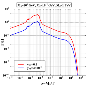
Figure 3: Lepton number conserving interaction rates (with out mixing one) comparison with Hubble expansion rate for two different couplings.

The produced lepton asymmetry is governed by Eq 16. Here the first term in the RHS is the source of the asymmetry, the second term involve different washout processes such as inverse decay, $\Delta L=1,\Delta L=2$ scatterings. The mixing angle $\theta_{s}$ plays important role in generating the lepton asymmetry. For very large mixing angle, the washout effects will be larger and for small mixing angles the washouts can be neglected and the lepton asymmetry will be produced by the late time decay of the $S$. In the following we discuss the lepton asymmetry generated in two separate cases, (i) large mixing angle ($10^{-3}\lesssim\theta_{s}\lesssim 0.1$), (ii) small mixing angle ($\theta_{s}<10^{-3}$).

Table 2: Benchmark points for leptogenesis

BPs	$M_{2}\rm(GeV)$	$M_{S}(\rm GeV)$	$M_{\rho}\rm(GeV)$	$z_{a}$	$(y^{\dagger}_{{}_{Nl}}y_{{}_{Nl}})_{22}$	$\theta_{s}$	$y_{{}_{NS}}$	$v_{\rho}\rm(GeV)$	$\epsilon_{S}$
BP1	$2\times 10^{12}$	$6\times 10^{7}$	$10^{3}$	$1+i0.1$	$3.1348\times 10^{-3}$	$10^{-3}$	$0.1$	$2.82834\times 10^{10}$	$5.9763\times 10^{-9}$
BP2	$1.3\times 10^{12}$	$2\times 10^{9}$	$10^{3}$	$1.3672+i3.3249\times 10^{-2}$	$2.1671\times 10^{-3}$	$7\times 10^{-3}$	$5\times 10^{-2}$	$2.56991\times 10^{11}$	$1.9921\times 10^{-7}$
BP3	$10^{12}$	$2\times 10^{9}$	$10^{3}$	$(50+i3)\times 10^{-3}$	$2.8938\times 10^{-4}$	$10^{-5}$	$0.42$	$3.36044\times 10^{7}$	$1.9921\times 10^{-7}$
BP4	$1.094\times 10^{12}$	$4.1\times 10^{8}$	$10^{3}$	$(4.808+i2.8955)\times 10^{-4}$	$3.1306\times 10^{-4}$	$6\times 10^{-4}$	$0.15$	$6.18503\times 10^{9}$	$4.0838\times 10^{-8}$

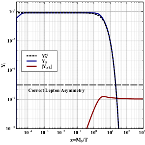
Figure 4: Cosmological evolution of lepton asymmetry for benchmark point BP1.

III.1 Large mixing angle ($10^{-3}\lesssim\theta_{s}\lesssim 0.1$)

We solve Eqs 15, and 16 with the BP1 parameters as mentioned in Table 2 considering the zero initial abundance of the $S$. Here to evaluate the Yukawa couplings we used the Casas-Ibarra (CI) parametrisation as mentioned in Equation 11 . The maximum CP asymmetry allowed for this $M_{S}$ is $\epsilon_{S}=5.9763\times 10^{-9}$. In Fig 4, we show the evolution of the asymmetry and the $S$ abundance as a function of $z$. The final lepton asymmetry is obtained to be $Y_{\Delta L}=1.09943\times 10^{-9}$, which is smaller than the required lepton asymmetry. The asymmetry is partially washed out in this scenario and also the CP asymmetry is very small to produce the required lepton asymmetry. Thus we conclude that such a choice of $M_{S}=6\times 10^{7}$ GeV can not giverise correct lepton asymmetry even if we choose the maximal CP-asymmetry. This implies that $M_{S}$ can not be lowered to an arbitrary small value in comparison to the Davidson-Ibarra bound ($M_{N}\gtrsim 2\times 10^{9}$ GeV). But we will see later that BP4 can give rise correct lepton asymmetry if $M_{S}\sim 4\times 10^{8}$ GeV which is one order of magnitude less than the DI bound on $M_{N}$.

Now we solve Eq 15, and 16 by fixing the parameters as mentioned in BP2 of Table 2. In this case, the maximum CP asymmetry is calculated to be $\epsilon_{S}=1.9921\times 10^{-7}$ which is one order larger compared to earlier case. Now using this sets of parameter, the final lepton asymmetry comes out to be $Y_{\Delta L}=3.18075\times 10^{-8}$, which satisfies the lepton asymmetry requirement as shown in Fig 5.

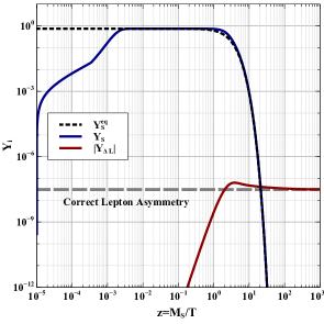
Figure 5: Cosmological evolution of lepton asymmetry for benchmark point BP2.

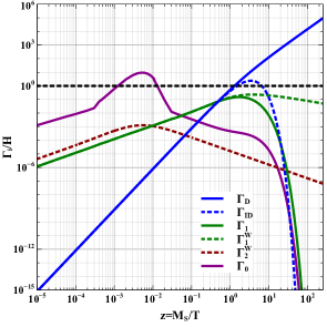
Figure 6: Cosmological evolution of various interaction rates are shown w.r.t. to Hubble rate for Benchmark point BP2.

In Fig 6, we show the evolution of the interaction rates for the BP2. Even if we started with the zero initial abundance of the $S$, we see that in the early time, the $\Delta L=0,1$ scattering processes along with the inverse decay help to increase the $S$ number density in the plasma. $S$ reaches equilibrium at $z\sim 3\times 10^{-3}$. Around $z\sim 1.3$ the inverse decay becomes larger than the Hubble rate, which brings back $S$ to equilibrium. Because of large inverse decay and $\Delta L=1$ washout processes, the lepton asymmetry gets washed out partially and settles to a final value which matches with the observed one.

III.2 Small mixing angle ($\theta_{s}<10^{-3}$)

In the case of small mixing angle the out-of-equilibrium decay happens at late epochs. At that time the washout processes will be no more active. For a good approximation we consider only decay, inverse decay and the scattering process which involve no mixing , e.g. $S\rho\rightarrow LH,SL\rightarrow\rho H,SH\rightarrow\rho L$ ($\Delta L=1$), $LH\rightarrow LH,LL\rightarrow HH$ ($\Delta L=2$), and $SS\rightarrow\rho\rho,S\rho\rightarrow S\rho$ ($\Delta L=0$). We solve the Boltzmann equations 15 and 16 with zero initial abundance of the $S$. Due to the $\Delta L=0$ processes $S$ will attain thermal equilibrium very quickly. It will stay in equilibrium due to the scatterings and inverse decay. Since, $S-N_{2}$ mixing angle is small, the out-of-equilibrium decay will happen at late epoch. However, we note that the mixing angle can not be arbitrarily small since the decay has to happen before the electroweak sphalerons freeze-out in order to give the required baryon asymmetry. One important consequence of small mixing angle is that it requires comparatively smaller vev of $\rho$. This results in gravitational waves in the nano Hz frequency range that we discuss in Section IV for BP3 from Table 2. As we see that for BP3 the $\rho$ obtains a vev around a scale of $\sim 10^{7}$ GeV which is below the mass scale of $S$. The mixing occurs at around $z\sim 10^{2}$ for BP3. For $z<10^{2}$, the $S$ reaches equilibrium only due to the $\Delta L=0$ processes as the mixing is absent. Once these processes fall below the Hubble rate, the $S$ abundance freezes out. We note that the freeze out abundance of $S$ is little less than the equilibrium value due to the annihilation process $S\bar{S}\rightarrow\rho\rho$. The $S$ is then mixes with the $N_{2}$ around $z\sim 10^{2}$, and it starts decaying to produce the lepton asymmetry. We show the evolution of the $S$ abundance as well as the lepton asymmetry yield in Fig 7. The final lepton asymmetry is found to be $Y_{\Delta L}=3.03897\times 10^{-8}$.

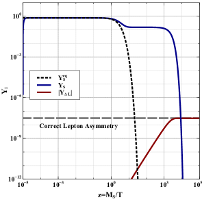
Figure 7: Cosmological evolution of lepton asymmetry for benchmark point BP3.

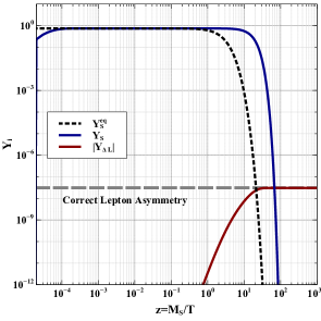
Figure 8: Cosmological evolution of lepton asymmetry for benchmark point BP4.

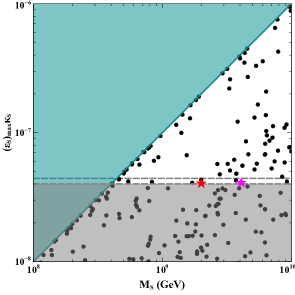
Figure 9: The value of $(\epsilon_{S})_{\rm max}\kappa_{S}$ as a function of $M_{S}$ is shown. The gray dashed line represents the value of $(\epsilon_{S})_{\rm max}\kappa_{S}=(4.215106\pm 0.207298)\times 10^{-8}$ which is required to produce the observed baryon asymmetry of the Universe.

We now take the BP4 from table 2 and solve the BEs. For the chosen parameters $S$ reaches equilibrium very early at around $z\sim 7\times 10^{-5}$ and it goes out-of-equilibrium at around $z\sim 1$. The $S$ then decays and produces the lepton asymmetry. Due to the small mixing angle the washout processes are negligible and thus we see no suppression in the final asymmetry. Here we found the final lepton asymmetry to be $Y_{\Delta L}=3.02967\times 10^{-8}$ for $M_{S}=4.1\times 10^{8}$ GeV.

We summarize our result in the plane of $(\epsilon_{S})_{\rm max}\kappa_{S}$ and $M_{S}$ in Fig 9. We vary the free parameters in the following range $M_{S}\in[10^{7},10^{10}]$ GeV, $M_{2}\in[2.4\times 10^{9},10^{14}]$ GeV, $M_{\rho}=10^{3}$ GeV, $z_{a}\in[0,360]+i[0,360]$, $\theta_{s}\in[10^{-6},0.1]$, $y_{{}_{NS}}\in[10^{-6},\sqrt{4\pi}]$. We also impose the condition $M_{2,3}>M_{S}$. The black points are obtained by solving the Boltzmann equations, 15, and 16. The gray dashed line is for $(\epsilon_{S})_{\rm max}\kappa_{S}=(4.215106\pm 0.207298)\times 10^{-8}$ which is required to produce the observed baryon asymmetry of the Universe. The gray shaded region is excluded as in this region the observed baryon asymmetry can not be sufficiently generated. On the other hand the points lying in the upper triangular white region are allowed because by choosing suitable values of the $\kappa_{S}$(strong washout) these points can be brought to the observable limit. Thus, we obtain the minimum value of $M_{S}$ which can give rise to observed baryon asymmetry as $M_{S}\simeq 4\times 10^{8}$ GeV. For $M_{S}<4\times 10^{8}$ GeV, the $(\epsilon_{S})_{\rm max}$ will not give rise to correct lepton asymmetry and this is evident from Eq 13. We note that this is one order magnitude smaller than the DI bound on the scale of thermal leptogenesis.

IV Domain walls and signatures of Gravitational waves from $Z_{2}$ symmetry breaking

The spontaneous breaking of $Z_{2}$ symmetry giving rise to lepton asymmetry also leads to formation of domain walls (DWs) in the early Universe. The energy density of the DWs falls with the cosmological scale factor as $\sim R^{-1}$, which is much slower than the matter ($\sim R^{-3}$) and radiation ($\sim R^{-4}$). Thus, the DWs may over close the Universe if they are stable. This problem can be solved by making the DW unstable and it will disappear eventually in the early Universe.

We demonstrate by considering the potential for the scalar fields as

$$V(\rho) = \frac{\lambda_{\rho}}{4}(\rho^{2}-v^{2}_{\rho})^{2}.$$ (17)

The potential has two degenerate minima at $<\rho>=\pm v_{\rho}$. The field can occupy any one of the two minima after the symmetry breaking resulting in two different domains, separated by a wall. We consider a static planar DW perpendicular to the $x$-axis in the Minkowski space, $\rho=\rho(x)$.

The equation of motion for the DW is [5, 8, 9, 55],

$$\frac{d^{2}\rho}{dx^{2}}-\frac{dV}{d\rho}=0,$$ (18)

with the boundary condition

$$\lim_{x\rightarrow\pm\infty}\rho(x)=\pm v_{\rho}.$$ (19)

After solving the equation of motion we obtain,

$$\rho(x)=v_{\rho}\tanh(\alpha x),$$ (20)

where $\alpha\simeq\sqrt{\frac{\lambda_{\rho}}{2}}v_{\rho}$.

The DW is extended along $x=0$ plane and the two vacua are realized at $x\rightarrow\pm\infty$. The width of the DW is estimated as $\delta\sim\big{(}\frac{\sqrt{\lambda_{\rho}}v_{\rho}}{\sqrt{2}}\big{)}^{-1}$. The surface energy density, also referred as tension of the DWs, is calculated to be ,

$$\sigma=\frac{4}{3}\sqrt{\frac{\lambda_{\rho}}{2}}v_{\rho}^{3}\simeq\frac{2}{3}M_{\rho}v^{2}_{\rho},$$ (21)

where $M_{\rho}=\sqrt{2\lambda_{\rho}}v_{\rho}$.

As discussed earlier without a soft $Z_{2}$ breaking term, the DW will be stable and will over close the energy density of the Universe. In order to over come this problem, we introduce an energy bias in the potential as $\mu^{3}_{b}\rho$, which breaks the $Z_{2}$ symmetry explicitly. Here $\mu_{b}$ is a mass dimension one coupling. The Eq 17 then becomes

$$\mathcal{V}=V(\rho)+\mu^{3}_{b}\rho.$$ (22)

As a result the degeneracy of the minima is lifted by

$$V_{bias}\equiv|\mathcal{V}(-v_{\rho})-\mathcal{V}(v_{\rho})|=\sqrt{2}\mu^{3}_{b}v_{\rho}.$$ (23)

This creates a pressure difference across the wall[8, 9, 55]. We assume the annihilation happens in the radiation dominated era. The energy bias has to be large enough, so that the DW can disappear before the BBN epoch, $\it{i.e.}$ $t_{ann}<t_{BBN}$, where

$$t_{ann}=\mathcal{C}_{ann}\frac{\mathcal{A}\sigma}{V_{bias}},$$ (24)

where $\mathcal{C}_{ann}$ is a coefficient of $\mathcal{O}(1)$, $\mathcal{A}\simeq 0.8\pm 0.1$[13] is area parameter, and $t_{BBN}$ is the BBN time scale. This gives a lower bound on the $V_{bias}$ as,

$$V_{bias}>6.58\times 10^{-14}{\rm GeV^{4}}\mathcal{C}_{ann}\mathcal{A}\bigg{(}\frac{10^{-2}{\rm sec}}{t_{BBN}}\bigg{)}\bigg{(}\frac{\sigma}{1{\rm TeV^{3}}}\bigg{)}.$$

(25)

Eq 25 can be written in terms of the $Z_{2}$ breaking parameters $\mu_{b}$ as

$$\mu_{b} > 1.45839\times 10^{-4}{\rm GeV}\mathcal{C}^{\frac{1}{3}}_{ann}\mathcal{A}^{\frac{1}{3}}\bigg{(}\frac{10^{-2}{\rm sec}}{t_{BBN}}\bigg{)}^{\frac{1}{3}}$$ (26)

$$\bigg{(}\frac{M_{\rho}}{1{\rm TeV}}\bigg{)}^{\frac{1}{3}}\bigg{(}\frac{v_{\rho}}{10^{5}{\rm TeV}}\bigg{)}^{\frac{1}{3}}.$$

Table 3: Benchmark points for Gravitation wave

BPs	$M_{2}\rm(GeV)$	$M_{S}(\rm GeV)$	$M_{\rho}\rm(GeV)$	$\theta_{s}$	$y_{{}_{NS}}$	$v_{\rho}\rm(GeV)$	$\sigma(\rm TeV^{3})$	$T_{ann}(\rm GeV)$
BPGW1	$10^{12}$	$2\times 10^{9}$	$10^{3}$	$10^{-5}$	$0.42$	$3.36044\times 10^{7}$	$7.52837\times 10^{8}$	$0.3$
BPGW2	$10^{12}$	$2\times 10^{9}$	$10^{3}$	$10^{-5}$	$0.42$	$3.36044\times 10^{7}$	$7.52837\times 10^{8}$	$0.5$
BPGW3	$4.008\times 10^{13}$	$4.09\times 10^{9}$	$10^{3}$	$4.7344\times 10^{-3}$	$1.2076\times 10^{-3}$	$2.2221\times 10^{14}$	$3.29188\times 10^{22}$	$2\times 10^{6}$

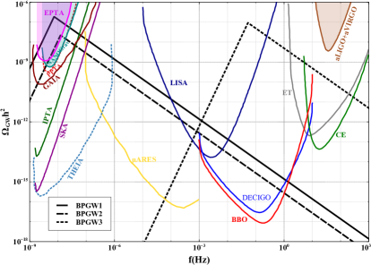
Figure 10: Gravitational wave spectrum from the annihilating domain walls for three benchmark points as mentioned in Table 3. Sensitivities from different gravitational wave search experiments have been shown with different colors.

The DWs has to disappear before they could start to dominate the energy density of the Universe, $\it i.e$ $t_{ann}<t_{dom}$, where

$$t_{dom}=\frac{3}{4}\frac{M_{pl}^{2}}{\mathcal{A}\sigma}.$$ (27)

This puts a lower bound on the annihilation temperature as,

$$T_{ann} > 1.34772{\rm GeV}\mathcal{A}^{1/2}\bigg{(}\frac{g_{*}(T_{ann})}{10}\bigg{)}^{-\frac{1}{4}}\bigg{(}\frac{v_{\rho}}{10^{5}{\rm TeV}}\bigg{)}$$ (28)

$$\bigg{(}\frac{M_{\rho}}{{1\rm TeV}}\bigg{)}^{\frac{1}{2}}.$$

Now in terms of $\mu_{b}$ it can be expressed as

$$\mu_{b} > 4.1404\times 10^{-3}{\rm GeV}\mathcal{C}_{ann}^{\frac{1}{3}}\mathcal{A}^{\frac{2}{3}}\bigg{(}\frac{M_{\rho}}{1{\rm TeV}}\bigg{)}^{\frac{2}{3}}\bigg{(}\frac{v_{\rho}}{10^{5}{\rm TeV}}\bigg{)}.$$

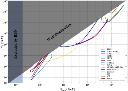
Figure 11: The sensitivity of the Gravitational Wave search experiments in the plane of $v_{\rho}-T_{ann}$ for $M_{\rho}=1$ TeV. These contours are obtained for peak frequency and peak amplitude of the GW as per Eq 31, and 30 respectively.

The DWs can then annihilate and emit their energy in the form of stochastic gravitational waves (GWs) which can be detectable at present time.

The peak amplitude of the GW spectrum at the present time, $t_{0}$, is given by[55]

$$\Omega_{GW}h^{2}(t_{0})|_{peak} = 7.18824\times 10^{-18}\mathcal{A}^{2}\tilde{\epsilon}_{GW}\bigg{(}\frac{\sigma}{1{\rm TeV^{3}}}\bigg{)}^{2}$$ (30)

$$\bigg{(}\frac{g_{*s}(T_{ann})}{10}\bigg{)}^{-\frac{4}{3}}\bigg{(}\frac{T_{ann}}{10^{-2}\rm GeV}\bigg{)}^{-4},$$

where $\tilde{\epsilon}_{GW}\simeq 0.7\pm 0.4$[13] is the efficiency parameter, $T_{ann}$ is the temperature at which the DWs annihilate, $g_{*s}(T_{ann})$ is the relativistic entropy degrees of freedom at the epoch of DWs annihilation.

From Eq 30, we see that the peak of GW spectrum is directly proportional to $\sigma^{2}$ and inversely proportional to $T_{ann}^{4}$. In our setup even though DW are produced before EW phase transition, they can sustain until late epoch to give rise larger peak amplitude of the GW spectrum. If the DW annihilation is happening at an earlier time i.e. at a large temperature, $T_{1}>T_{2}$, then the amplitude of the GW will be larger for $T_{2}$ as compared to $T_{1}$.

Assuming the DW disappear at temperature $T_{ann}$, the peak frequency of the GW spectrum at present time is estimated as

$$f_{peak}(t_{0}) = 1.78648\times 10^{-10}{\rm Hz}\bigg{(}\frac{g_{*s}(T_{ann})}{10}\bigg{)}^{-\frac{1}{3}}$$ (31)

$$\bigg{(}\frac{g_{*}(T_{ann})}{10}\bigg{)}^{\frac{1}{2}}\bigg{(}\frac{T_{ann}}{10^{-2}\rm GeV}\bigg{)}.$$

Now the amplitude of the GW for any frequency at the present time varies as

$$\Omega_{GW}(t_{0},f)=\Omega_{GW}h^{2}(t_{0})|_{peak}\left\{\begin{array}[]{l}\frac{f_{peak}}{f}~{}~{}~{}~{}~{}~{}~{}~{}~{}~{}~{}~{}f>f_{peak}\\ \bigg{(}\frac{f}{f_{peak}}\bigg{)}^{3}~{}~{}~{}~{}f<f_{peak}.\\ \end{array}\right.$$ (32)

It is worth mentioning that $v_{\rho}$ is the only parameter which is sensitive to both the leptogenesis and GW spectrum. In Fig 10, we have illustrated the GW spectrum for 3 benchmark values of $T_{ann}$ as mentioned in Table 3. BPGW1 and BPGW2 is shown as red “star”in Fig 9 and BPGW3 as magenta colored “star”in Fig 9. We have used 3 benchmark values of $T_{ann}$ as 0.3 GeV, 0.5 GeV, and $2\times 10^{6}$ GeV for BPGW1, BPGW2, and BPGW3 respectively. We have shown different sensitivities from experiments BBO[56], CE, DECIGO[57], NANOGrav[1, 2], EPTA [3], CPTA [58] , PPTA [4], ET[59], GAIA[60], IPTA [61], LISA, SKA[62], THEIA[60], aLIGO [63], aVIRGO, $\mu$ARES[64]. The peak frequencies lie around the nano Hz frequency range as observed by NANOGrav, EPTA, PPTA for the BPGW1 and BPGW2. For BPGW3 the frequency lies around mili Hz to Hz which is sensitive to LISA.

We have shown the sensitivity reaches of different experiments in the plane of $v_{\rho}$ verses $T_{ann}$ for a fixed $\rho$ mass, $M_{\rho}=1$ TeV in Fig 11. The parameter space is constrained by the facts that the DWs must annihilate before BBN and before they will dominate the energy density of the Universe.

V Dark Matter phenomenology

Now we turn to comment on DM in our setup. Due to the unbroken $Z_{2}^{\prime}$ symmetry combination of $N_{1}$ and $\Psi=(\psi^{0}~{}~{}\psi^{-})^{T}\equiv(\psi_{L}^{0}+\psi_{R}^{0}~{}~{}\psi^{-})^{T}$ can give rise to a singlet-doublet Majorana DM[38]. The relevant DM Lagrangian reads as

$$\mathcal{L}_{\rm DM} = \overline{\Psi}i\gamma^{\mu}\mathcal{D}_{\mu}\Psi-M\bar{\Psi}\Psi+\overline{N_{1}}i\gamma^{\mu}\partial_{\mu}N_{1}-\frac{1}{2}M_{1}\overline{N^{c}_{1}}N_{1}$$

$$- \frac{y_{1}}{\sqrt{2}}\overline{\Psi}\tilde{H}(N_{1}+N^{c}_{1})+h.c..$$

The neutral fermion mass matrix can be written in the basis: $((\psi^{0}_{R})^{c},\psi^{0}_{L},(N_{1})^{c})^{T}$ as

$$\begin{pmatrix}0&M&\frac{m_{D}}{\sqrt{2}}\\ M&0&\frac{m_{D}}{\sqrt{2}}\\ \frac{m_{D}}{\sqrt{2}}&\frac{m_{D}}{\sqrt{2}}&M_{1}\end{pmatrix},$$ (34)

where $m_{D}=y_{1}v_{h}/\sqrt{2}$. The mass matrix can be diagonalised with a unitary matrix of the form $U(\theta)=U_{13}(\theta_{13}=\theta).U_{23}(\theta_{23}=0).U_{12}(\theta_{12}=\frac{\pi}{4})$. The three neutral states mix and gives three Majorana states as $\chi_{i}=\frac{\chi_{iL}+\chi_{iL}^{c}}{\sqrt{2}}$, where

$$\chi_{1L} = \frac{\cos\theta}{\sqrt{2}}(\psi^{0}_{L}+(\psi^{0}_{R})^{c})+\sin\theta N_{1}^{c},$$

$$\chi_{2L} = \frac{i}{\sqrt{2}}(\psi^{0}_{L}-(\psi^{0}_{R})^{c}),$$

$$\chi_{3L} = -\frac{\sin\theta}{\sqrt{2}}(\psi^{0}_{L}+(\psi^{0}_{R})^{c})+\cos\theta N_{1}^{c}.$$ (35)

The corresponding mass eigen values are

$$M_{\chi_{1}} = M\cos^{2}\theta+M_{1}\sin^{2}\theta+m_{D}\sin 2\theta,$$

$$M_{\chi_{2}} = M,$$

$$M_{\chi_{3}} = M\sin^{2}\theta+M_{1}\cos^{2}\theta-m_{D}\sin 2\theta,$$ (36)

where the mixing angle is given as

$$\tan 2\theta=\frac{2m_{D}}{M-M_{1}}.$$ (37)

Here we identify the $\chi_{3}$ be DM candidate. The Yukawa coupling can be expressed as,

$$y_{1}=\frac{\Delta M\sin 2\theta}{\sqrt{2}v_{h}},$$ (38)

where $\Delta M$ is the mass splitting between DM and the next heavy neutral fermion state. The free parameters in the DM phenomenology are $\{M_{\chi_{3}}\equiv M_{DM},\Delta M=M_{\chi_{1}}-M_{\chi_{3}}\approx M_{\chi_{2}}-M_{\chi_{3}},\sin\theta\}$.

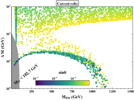
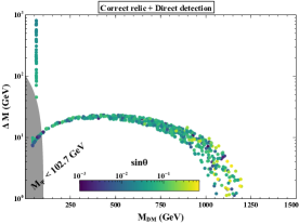
Figure 12: [Left]: DM parameter space satisfying correct relic in the plane of $\Delta M$ vs $M_{\rm DM}$. [Right]: Parameter space consistent with both relic density and Direct Search constraints (LZ) in the $\Delta M$ versus $M_{\rm DM}$ plane. The gray shaded region in the bottom left corner is ruled out by the LEP exclusion bound on charged fermion mass $M_{\Psi^{+}}\equiv M>$ 102.7 GeV.

The DM relic is decided by the freeze-out of various annihilation and co-annihilation processes in the early Universe. We compute the relic density and the DM spin independent cross-section using the micrOMEGAs package [65]. In Fig 12 [left], we show the mass splitting between the DM and the light neutral fermion as a function of DM mass for correct relic density. As the DM mass increases, the annihilation cross-section decreases, and as a result the relic increases. Now co-annihilation plays important role in bringing down the relic to correct ball park. The co-annihilation is large when the mass splitting between the DM and the next $Z_{2}^{\prime}$ odd sector particle is smaller. This feature is clearly visible in Fig 12 [left]. When the mass splitting $\Delta M$ is large, co-annihilation becomes negligible. The Higgs mediated annihilation processes decide the relic density mainly. Thus the mixing angle $\sin\theta$ becomes important here as the Yukawa coupling is $\propto\Delta M\sin 2\theta$. The dependence of mixing angle for large mass splitting is prominent in Fig 12 [left]. For fixed $\sin\theta$, as the mass splitting increases, the coupling increases which leads to increase in annihilation cross-section and thus the relic decreases. Now to get correct relic, the DM mass has to be large, which makes the cross-section smaller giving correct relic. Larger $\sin\theta$ requires smaller $\Delta M$ to give correct relic. Now we take these correct relic data points and impose the direct detection constraint from LZ experiment [66] and show in Fig 12 [right]. The direct detection is possible via the Higgs portal. The spin-independent DM-nucleon cross-section is $\sigma^{SI}_{DM-N}\propto y^{2}_{1}\sin^{2}2\theta\propto\Delta M^{2}\sin^{4}2\theta$. Larger mixing angle as well as larger mass splitting will result in larger direct detection cross-section. However, larger mass splitting is allowed for DM mass at Higgs resonance. We also impose the LEP bound on the mass of the charged component of the doublet, which is $M_{\Psi^{+}}>102.7$ GeV [67].

VI Conclusion

In this paper, we explored the potential for generating successful thermal leptogenesis at a scale lower than the Davidson Ibarra bound in an extended type-I seesaw framework along with non-zero neutrino mass, dark matter and gravitational wave. In our setup the lightest RHN $N_{1}$ mixes with the neutral component of a vector like fermion doublet $\Psi$ which are odd under an unbroken $Z_{2}^{\prime}$ symmetry. As a result we get singlet-doublet Majorana DM in a wide range of parameter space. We also added a singlet scalar $\rho$ and a singlet fermion $S$ in the canonical type-I seesaw which are odd under an imposed discrete $Z_{2}$ symmetry. At high scale, typically above the EWPT $\rho$ acquires a vev and breaks the $Z_{2}$ symmetry spontaneously. As a result we got $S$ mixed up with $N_{2}$ such that late decay of $S$ could give rise to a relatively low scale thermal leptogenesis. In particular we saw that successful thermal leptogenesis requires $M_{S}\gtrsim 4\times 10^{8}$ GeV. We note that this is one order magnitude smaller than the usual Davidson Ibarra bound ($M_{N}>2.4\times 10^{9}$ GeV). The spontaneous breaking of the $Z_{2}$ symmetry also gave rise DWs in the early Universe. We discussed the evolution of the DWs which disappear by emitting stochastic GWs. We saw that in appropriate parameter space they can give rise signatures at various GW experiments like NANOGrav, EPTA, PPTA, LISA etc.

Appendix A Lower bound on the leptogenesis scale in canonical type-I seesaw

In the hierarchical scenario of the canonical type-I leptogenesis the lightest RHN decays to $L,H$ and $\bar{L},H^{\dagger}$. The interference between these tree level and one loop processes can give rise to a CP asymmetry given as

$$\epsilon_{{}_{N_{1}}}=-\frac{3}{8\pi v_{h}^{2}}M_{1}\sum_{j=2,3}\frac{1}{M_{j}}\frac{Im[(m^{\dagger}_{D}m_{D})_{1j}]^{2}}{(m^{\dagger}_{D}m_{D})_{11}},$$ (39)

where $v_{h}=246$ GeV, is the SM Higgs vev.

The decay width of $N_{1}$ is calculated to be,

$$\Gamma_{{}_{N_{1}}}=\frac{(m^{\dagger}_{D}m_{D})_{11}}{8\pi v_{h}^{2}}M_{{1}}.$$ (40)

Now a net lepton asymmetry can be generated once this decay rate falls below the Hubble expansion rate of the Universe,

$${\rm\bf{H}}(T)=1.66\sqrt{g_{*}}\frac{T^{2}}{M_{pl}},$$ (41)

where $g_{*}$ is the effective number of relativistic degrees of freedom, $M_{pl}=1.22\times 10^{19}$ GeV is the Planck mass.

The CP asymmetry is bounded from above as [50]

$$\epsilon_{{}_{N_{1}}}\leq\frac{3}{8\pi v_{h}^{2}}M_{1}\sqrt{\Delta m^{2}_{atm}}.$$ (42)

In the zero initial abundance case the lower bound on the lightest RHN mass is found to be [68]

$$M_{1}\gtrsim 2.4\times 10^{9}~{}{\rm GeV}.$$ (43)

This is mainly because the same coupling is responsible to give neutrino mass as well as leptogenesis. Various attempts have been made to lower this leptogenesis scale, e.g. incorporating flavor effects [75], by adding extra scalar fields [76, 77, 78], resonant leptogensis [79], and by decoupling neutrino mass and leptogenesis [48, 49].

References

- Agazie et al. [2023] G. Agazie et al. (NANOGrav), Astrophys. J. Lett. 951, L8 (2023), arXiv:2306.16213 [astro-ph.HE] .
- Afzal et al. [2023] A. Afzal et al. (NANOGrav), Astrophys. J. Lett. 951, L11 (2023), arXiv:2306.16219 [astro-ph.HE] .
- Antoniadis et al. [2023] J. Antoniadis et al. (EPTA, InPTA:), Astron. Astrophys. 678, A50 (2023), arXiv:2306.16214 [astro-ph.HE] .
- Reardon et al. [2023] D. J. Reardon et al., Astrophys. J. Lett. 951, L6 (2023), arXiv:2306.16215 [astro-ph.HE] .
- Vilenkin and Shellard [2000] A. Vilenkin and E. P. S. Shellard, Cosmic Strings and Other Topological Defects (Cambridge University Press, 2000).
- Zeldovich et al. [1974] Y. B. Zeldovich, I. Y. Kobzarev, and L. B. Okun, Zh. Eksp. Teor. Fiz. 67, 3 (1974).
- Vilenkin [1981] A. Vilenkin, Phys. Rev. D 23, 852 (1981).
- Gelmini et al. [1989] G. B. Gelmini, M. Gleiser, and E. W. Kolb, Phys. Rev. D 39, 1558 (1989).
- Larsson et al. [1997] S. E. Larsson, S. Sarkar, and P. L. White, Phys. Rev. D 55, 5129 (1997), arXiv:hep-ph/9608319 .
- Gleiser and Roberts [1998] M. Gleiser and R. Roberts, Phys. Rev. Lett. 81, 5497 (1998), arXiv:astro-ph/9807260 .
- Hiramatsu et al. [2010] T. Hiramatsu, M. Kawasaki, and K. Saikawa, JCAP 05, 032, arXiv:1002.1555 [astro-ph.CO] .
- Kawasaki and Saikawa [2011] M. Kawasaki and K. Saikawa, JCAP 09, 008, arXiv:1102.5628 [astro-ph.CO] .
- Hiramatsu et al. [2014] T. Hiramatsu, M. Kawasaki, and K. Saikawa, JCAP 02, 031, arXiv:1309.5001 [astro-ph.CO] .
- Bhattacharya et al. [2024] S. Bhattacharya, N. Mondal, R. Roshan, and D. Vatsyayan, JCAP 06, 029, arXiv:2312.15053 [hep-ph] .
- Borah and Dasgupta [2022] D. Borah and A. Dasgupta, Phys. Rev. D 106, 035016 (2022), arXiv:2205.12220 [hep-ph] .
- Barman et al. [2022] B. Barman, D. Borah, A. Dasgupta, and A. Ghoshal, Phys. Rev. D 106, 015007 (2022), arXiv:2205.03422 [hep-ph] .
- Minkowski [1977] P. Minkowski, Phys. Lett. B 67, 421 (1977).
- Mohapatra and Senjanovic [1981] R. N. Mohapatra and G. Senjanovic, Phys. Rev. D 23, 165 (1981).
- Mohapatra and Pal [1991] R. N. Mohapatra and P. B. Pal, Massive neutrinos in physics and astrophysics, Vol. 41 (1991).
- Mahbubani and Senatore [2006] R. Mahbubani and L. Senatore, Phys. Rev. D73, 043510 (2006), arXiv:hep-ph/0510064 [hep-ph] .
- D’Eramo [2007] F. D’Eramo, Phys. Rev. D76, 083522 (2007), arXiv:0705.4493 [hep-ph] .
- Cohen et al. [2012] T. Cohen, J. Kearney, A. Pierce, and D. Tucker-Smith, Phys. Rev. D85, 075003 (2012), arXiv:1109.2604 [hep-ph] .
- Freitas et al. [2015] A. Freitas, S. Westhoff, and J. Zupan, JHEP 09, 015, arXiv:1506.04149 [hep-ph] .
- Cynolter et al. [2016] G. Cynolter, J. Kovács, and E. Lendvai, Mod. Phys. Lett. A31, 1650013 (2016), arXiv:1509.05323 [hep-ph] .
- Calibbi et al. [2015] L. Calibbi, A. Mariotti, and P. Tziveloglou, JHEP 10, 116, arXiv:1505.03867 [hep-ph] .
- Cheung and Sanford [2014] C. Cheung and D. Sanford, JCAP 1402, 011, arXiv:1311.5896 [hep-ph] .
- Enberg et al. [2007] R. Enberg, P. J. Fox, L. J. Hall, A. Y. Papaioannou, and M. Papucci, JHEP 11, 014, arXiv:0706.0918 [hep-ph] .
- Banerjee et al. [2016] S. Banerjee, S. Matsumoto, K. Mukaida, and Y.-L. S. Tsai, JHEP 11, 070, arXiv:1603.07387 [hep-ph] .
- Dutta Banik et al. [2018] A. Dutta Banik, A. K. Saha, and A. Sil, Phys. Rev. D98, 075013 (2018), arXiv:1806.08080 [hep-ph] .
- Horiuchi et al. [2016] S. Horiuchi, O. Macias, D. Restrepo, A. Rivera, O. Zapata, and H. Silverwood, JCAP 03, 048, arXiv:1602.04788 [hep-ph] .
- Restrepo et al. [2015] D. Restrepo, A. Rivera, M. Sánchez-Peláez, O. Zapata, and W. Tangarife, Phys. Rev. D92, 013005 (2015), arXiv:1504.07892 [hep-ph] .
- Abe [2017] T. Abe, Phys. Lett. B 771, 125 (2017), arXiv:1702.07236 [hep-ph] .
- Bhattacharya et al. [2017a] S. Bhattacharya, N. Sahoo, and N. Sahu, Phys. Rev. D96, 035010 (2017a), arXiv:1704.03417 [hep-ph] .
- Bhattacharya et al. [2019] S. Bhattacharya, P. Ghosh, and N. Sahu, JHEP 02, 059, arXiv:1809.07474 [hep-ph] .
- Bhattacharya et al. [2017b] S. Bhattacharya, B. Karmakar, N. Sahu, and A. Sil, JHEP 05, 068, arXiv:1611.07419 [hep-ph] .
- Bhattacharya et al. [2016] S. Bhattacharya, N. Sahoo, and N. Sahu, Phys. Rev. D 93, 115040 (2016), arXiv:1510.02760 [hep-ph] .
- Bhattacharya et al. [2018] S. Bhattacharya, P. Ghosh, N. Sahoo, and N. Sahu, (2018), arXiv:1812.06505 [hep-ph] .
- Dutta et al. [2021] M. Dutta, S. Bhattacharya, P. Ghosh, and N. Sahu, JCAP 03, 008, arXiv:2009.00885 [hep-ph] .
- Borah et al. [2021a] D. Borah, M. Dutta, S. Mahapatra, and N. Sahu, (2021a), arXiv:2109.02699 [hep-ph] .
- Borah et al. [2021b] D. Borah, M. Dutta, S. Mahapatra, and N. Sahu, (2021b), arXiv:2112.06847 [hep-ph] .
- Borah et al. [2022] D. Borah, S. Mahapatra, and N. Sahu, Phys. Lett. B 831, 137196 (2022), arXiv:2204.09671 [hep-ph] .
- Borah et al. [2024a] D. Borah, S. Mahapatra, D. Nanda, S. K. Sahoo, and N. Sahu, JHEP 05, 096, arXiv:2310.03721 [hep-ph] .
- Kibble [1976] T. W. B. Kibble, J. Phys. A 9, 1387 (1976).
- Kibble et al. [1982] T. W. B. Kibble, G. Lazarides, and Q. Shafi, Phys. Rev. D 26, 435 (1982).
- Lazarides et al. [1982] G. Lazarides, Q. Shafi, and T. F. Walsh, Nucl. Phys. B 195, 157 (1982).
- Vilenkin [1985] A. Vilenkin, Phys. Rept. 121, 263 (1985).
- Casas and Ibarra [2001] J. A. Casas and A. Ibarra, Nucl. Phys. B618, 171 (2001), arXiv:hep-ph/0103065 [hep-ph] .
- Ma et al. [2007] E. Ma, N. Sahu, and U. Sarkar, J. Phys. G 34, 741 (2007), arXiv:hep-ph/0611257 .
- Ma et al. [2006] E. Ma, N. Sahu, and U. Sarkar, J. Phys. G 32, L65 (2006), arXiv:hep-ph/0603043 .
- Davidson and Ibarra [2002] S. Davidson and A. Ibarra, Phys. Lett. B535, 25 (2002), arXiv:hep-ph/0202239 [hep-ph] .
- Borah et al. [2024b] D. Borah, S. Mahapatra, P. K. Paul, N. Sahu, and P. Shukla, Phys. Rev. D 110, 035033 (2024b), arXiv:2404.14912 [hep-ph] .
- Aghanim et al. [2020] N. Aghanim et al. (Planck), Astron. Astrophys. 641, A6 (2020), [Erratum: Astron.Astrophys. 652, C4 (2021)], arXiv:1807.06209 [astro-ph.CO] .
- Buchmuller et al. [2005] W. Buchmuller, P. Di Bari, and M. Plumacher, Annals Phys. 315, 305 (2005), arXiv:hep-ph/0401240 [hep-ph] .
- de Salas et al. [2021] P. F. de Salas, D. V. Forero, S. Gariazzo, P. Martínez-Miravé, O. Mena, C. A. Ternes, M. Tórtola, and J. W. F. Valle, JHEP 02, 071, arXiv:2006.11237 [hep-ph] .
- Saikawa [2017] K. Saikawa, Universe 3, 40 (2017), arXiv:1703.02576 [hep-ph] .
- Yunes and Berti [2008] N. Yunes and E. Berti, Phys. Rev. D 77, 124006 (2008), [Erratum: Phys.Rev.D 83, 109901 (2011)], arXiv:0803.1853 [gr-qc] .
- Adelberger et al. [2006] E. G. Adelberger, N. A. Collins, and C. D. Hoyle, Class. Quant. Grav. 23, 125 (2006), [Erratum: Class.Quant.Grav. 23, 5463 (2006), Erratum: Class.Quant.Grav. 38, 059501 (2021)], arXiv:gr-qc/0512055 .
- Xu et al. [2023] H. Xu et al., Res. Astron. Astrophys. 23, 075024 (2023), arXiv:2306.16216 [astro-ph.HE] .
- Punturo et al. [2010] M. Punturo et al., Class. Quant. Grav. 27, 194002 (2010).
- Garcia-Bellido et al. [2021] J. Garcia-Bellido, H. Murayama, and G. White, JCAP 12 (12), 023, arXiv:2104.04778 [hep-ph] .
- Hobbs et al. [2010] G. Hobbs et al., Class. Quant. Grav. 27, 084013 (2010), arXiv:0911.5206 [astro-ph.SR] .
- Weltman et al. [2020] A. Weltman et al., Publ. Astron. Soc. Austral. 37, e002 (2020), arXiv:1810.02680 [astro-ph.CO] .
- Aasi et al. [2015] J. Aasi et al. (LIGO Scientific), Class. Quant. Grav. 32, 074001 (2015), arXiv:1411.4547 [gr-qc] .
- Sesana et al. [2021] A. Sesana et al., Exper. Astron. 51, 1333 (2021), arXiv:1908.11391 [astro-ph.IM] .
- Alguero et al. [2024] G. Alguero, G. Belanger, F. Boudjema, S. Chakraborti, A. Goudelis, S. Kraml, A. Mjallal, and A. Pukhov, Comput. Phys. Commun. 299, 109133 (2024), arXiv:2312.14894 [hep-ph] .
- Aalbers et al. [2023] J. Aalbers et al. (LZ), Phys. Rev. Lett. 131, 041002 (2023), arXiv:2207.03764 [hep-ex] .
- Abdallah et al. [2003] J. Abdallah et al. (DELPHI), Eur. Phys. J. C 31, 421 (2003), arXiv:hep-ex/0311019 .
- Buchmuller et al. [2002] W. Buchmuller, P. Di Bari, and M. Plumacher, Nucl. Phys. B643, 367 (2002), [Erratum: Nucl. Phys.B793,362(2008)], arXiv:hep-ph/0205349 [hep-ph] .
- Khlopov and Linde [1984] M. Y. Khlopov and A. D. Linde, Phys. Lett. B 138, 265 (1984).
- Ellis et al. [1984] J. R. Ellis, J. E. Kim, and D. V. Nanopoulos, Phys. Lett. B 145, 181 (1984).
- Ellis et al. [1985] J. R. Ellis, D. V. Nanopoulos, and S. Sarkar, Nucl. Phys. B 259, 175 (1985).
- Bolz et al. [2001] M. Bolz, A. Brandenburg, and W. Buchmuller, Nucl. Phys. B 606, 518 (2001), [Erratum: Nucl.Phys.B 790, 336–337 (2008)], arXiv:hep-ph/0012052 .
- Kawasaki et al. [2005] M. Kawasaki, K. Kohri, and T. Moroi, Phys. Rev. D 71, 083502 (2005), arXiv:astro-ph/0408426 .
- Allahverdi and Mazumdar [2006] R. Allahverdi and A. Mazumdar, JCAP 10, 008, arXiv:hep-ph/0512227 .
- Blanchet and Di Bari [2009] S. Blanchet and P. Di Bari, Nucl. Phys. B 807, 155 (2009), arXiv:0807.0743 [hep-ph] .
- Clarke et al. [2015] J. D. Clarke, R. Foot, and R. R. Volkas, Phys. Rev. D 92, 033006 (2015), arXiv:1505.05744 [hep-ph] .
- Hugle et al. [2018] T. Hugle, M. Platscher, and K. Schmitz, Phys. Rev. D 98, 023020 (2018), arXiv:1804.09660 [hep-ph] .
- Vatsyayan and Goswami [2023] D. Vatsyayan and S. Goswami, Phys. Rev. D 107, 035014 (2023), arXiv:2208.12011 [hep-ph] .
- Pilaftsis and Underwood [2004] A. Pilaftsis and T. E. J. Underwood, Nucl. Phys. B692, 303 (2004), arXiv:hep-ph/0309342 [hep-ph] .