Modeling Advection-Dominated Flows with Space-Local Reduced-Order Models

Abstract

Reduced-order models (ROMs) are often used to accelerate the simulation of large physical systems. However, traditional ROM techniques, such as those based on proper orthogonal decomposition (POD), often struggle with advection-dominated flows due to the slow decay of singular values. This results in high computational costs and potential instabilities.

This paper proposes a novel approach using space-local POD to address the challenges arising from the slow singular value decay. Instead of global basis functions, our method employs local basis functions that are applied across the domain, analogous to the finite element method. By dividing the domain into subdomains and applying a space-local POD within each subdomain, we achieve a representation that is sparse and that generalizes better outside the training regime. This allows the use of a larger number of basis functions, without prohibitive computational costs. To ensure smoothness across subdomain boundaries, we introduce overlapping subdomains inspired by the partition of unity method.

Our approach is validated through simulations of the 1D advection equation discretized using a central difference scheme. We demonstrate that using our space-local approach we obtain a ROM that generalizes better to flow conditions which are not part of the training data. In addition, we show that the constructed ROM inherits the energy conservation and non-linear stability properties from the full-order model. Finally, we find that using a space-local ROM allows for larger time steps.

1 Introduction

Simulating large physical systems is an ongoing challenge in the field of computational sciences. This especially becomes challenging when dealing with multiscale systems. Such systems are characterized by displaying interesting behavior at different scales of space/time. A prominent example and our main incentive for this work are turbulent flows described by the incompressible Navier-Stokes equations. Systems described by these equations feature the formation of turbulent eddies of a range of different sizes. The large difference in size between the largest and the smallest eddies gives rise to the multiscale nature of the problem. The problem with simulating such systems is that they require high resolution computational meshes to obtain accurate simulations, and small time steps. This places a huge burden on the available computational resources [1, 2].

To make simulation of turbulent flows feasible one typically resorts to Reynolds averaged Navier-Stokes [3], large eddy simulation [4], and reduced-order models (ROMs)[5, 6]. Here we focus on the latter approach. In reduced-order modelling, data is used to speed up simulations. The data can both be obtained from simulations or experiments. The collected data is then used to identify the most important features of the flow. This is typically done by a proper orthogonal decomposition (POD)of the collected flow data. The resulting features are then used to construct a reduced basis. By projecting the fluid flow equations on this basis one obtains the widely used POD-Galerkin ROM [7, 8, 6]. However, two common issues with POD-Galerkin ROMs are their stability and their accuracy for convection-dominated systems. In [9] it is shown that the stability issue can be resolved by making sure that the energy-conserving property of the Navier-Stokes equations is still satisfied under Galerkin projection. For the incompressible Navier-Stokes equations, the only prerequisite for an energy-conserving ROM is that the discretization is structure-preserving, i.e. it is such that it inherits the energy conservation property from the continuous equations.

However, the stability property derived in [9] does not guarantee accuracy – it is possible to have energy-stable simulations that are highly inaccurate. This issue can already be observed on academic test cases such as the linear advection equation. For example, in [5] the authors discuss the problem of a single traveling wave, through a periodic domain. Even though it is clear that a one dimensional representation of the system exists, it is not recovered by the POD algorithm. The result is a slow decay in singular values of the snapshot matrix. This means that many POD modes are required to accurately describe the flow. The slow decay in singular values is often related to the Kolmogorov $N$-width. This is a measure of how well the solution space of a partial differential equation (PDE) can be represented by a linear combination of $N$ basis functions [10, 11]. Advection-dominated flows are notorious for displaying a slow Kolmogorov $N$-width decay, requiring a large $N$ for accurate simulation. The resulting ROM is then expensive to evaluate [12, 13]. When not including sufficient number of basis functions inaccurate results are obtained, e.g. they contain oscillations [14, 15].

Different approaches to deal with this problem have been suggested. One way of dealing with this is by taking a local in time approach [16]. In this approach the ROM switches basis for different time intervals. This means that the ROM can employ a smaller basis, since each basis is specialized to deal with a certain time interval. Switching between basis during simulation can also be done in a structure-preserving (energy-conserving) manner [17]. A related approach is updating the basis during the ROM simulation to be more robust to changes in simulation conditions [18]. In [19] a Petrov-Galerkin approach is suggested, which leads to more stable ROMs when using a small POD basis than the standard Galerkin approach. In [20] it is suggested to add a closure model to the ROM to account for a small POD basis. The closure model is then tasked with modeling the interaction between the part of the flow that is covered by the POD basis and the part which is removed. Another suggestion is to construct ROMs on nonlinear reduced subspaces instead of linear ones. In [21] a more accurate representation of the solution space is obtained using rational quadratic manifolds. Here the ROM construction was also performed in a structure-preserving (entropy-stable) manner, yielding stability of the ROM.

Machine learning approaches have also gained traction for the construction of ROMs. In [22] a long short-term memory (LSTM) neural network is used instead of Galerkin projection, as the computational complexity of LSTM is more favorable than Galerkin projection-based ROMs. They also allow one to take larger time steps [23]. In [23] this approach is combined with an autoencoder to reduce the dimensionality of the system. It is shown that a much greater reduction in degrees of freedom (DOF) can be reached using this approach compared to the standard POD-Galerkin approach. In [10] an advection-aware autoencoder is suggested to reduced the dimensionality of this system. This is achieved by introducing an additional decoder which is trained to reconstruct a “shifted” version of the encoded snapshots. This shift can for example be a snapshot taken further in time. This forces the latent space of the autoencoder to become aware of the dominant advective features of the flow.

In this work we focus on another approach to tackle the issue of ROM accuracy in advection-dominated flows. Similar to [24] the idea is to use a POD approach to obtain a “space-local reduced-order basis”. In contrast to the standard POD procedure, which results in global basis functions, the resulting basis has local support. This means the basis functions are only nonzero on part of the domain. The advantage of this is that the resulting Galerkin projected operators are sparse. This makes them much cheaper to evaluate when simulating the ROM. For example, in [24] a speedup of up to 1.5 orders of magnitude is reported with respect to a standard POD-Galerkin ROM. We propose to use this idea of a space-local POD to tackle the slow singular value decay of advection-dominated flows. The idea is as follows: instead of obtaining a set of global basis functions which span the entire domain, we obtain a set of space-local basis functions. These basis functions are then “copy pasted” across the entire domain, similarly to how a finite element basis covers the domain [25]. These basis functions are only nonzero on their designated subdomain. Our approach differs from the one presented in [24]: in our approach, the solution data in each of the subdomains is treated with the same local basis in our local POD, instead of obtaining a different local POD basis for each subdomain as in [24]. This means that a feature observed in part of the domain, can also be represented on a different part of the domain, by the same basis. In this way, less data is required to obtain a POD basis that generalizes well. Note that while this procedure does not solve the slow Kolmogorov $N$-width decay (we still use linear approximations), the sparsity of the basis allows us to use a much larger number of basis functions.

Sparsity and generalizability are therefore key features of our approach. In addition, we add two further novel ideas in this work: the use of overlapping subdomains (to avoid discontinuities at the subdomain boundaries), and enforcing energy conservation for our space-local ROM, such that stability is guaranteed.

This paper is structured in the following way. In section 2 we introduce the full-order model (FOM), namely a central difference discretization of the 1D advection equation. The central difference discretization ensures the scheme is energy conserving. In section 3 we introduce the POD approaches. With start off with the standard POD approach and then introduce our space-local approaches, with and without overlapping subdomains. In section 4 we use Galerkin projection to project the FOM onto the POD basis and show that the resulting ROMs satisfy energy conservation. Finally, in section 5 we evaluate the different POD-based approaches based on a set of different metrics. The different POD approaches are judged on the ability to represent the solution. Next, we evaluate the performance of the ROMs on a simulation, extrapolating beyond the data used for the POD. In addition, we investigate how well energy conservation is satisfied. To conclude this section we analyze the computational cost of the ROMs. Finally in section 6, we present our main conclusions and suggest future research topics.

2 Full-order model

2.1 Advection equation

In this work we are concerned with developing a reduced-order model for the linear advection equation. This equation is chosen as it exhibits similar difficulties as the incompressible Navier-Stokes equations when applying model reduction. We consider a scalar solution $u(x,t)$ to the linear advection equation

$$\frac{\partial u}{\partial t}=-c\frac{\partial u}{\partial x},$$ (1)

with initial condition $u(x,0)=u_{0}(x)$ and constant $c$. We employ a periodic domain $\Omega$ such that we do not require boundary conditions (BCs). An important property of this equation is that the total energy of the system

$$E:=\frac{1}{2}(u,u),$$ (2)

is conserved, where

$$(a(x),b(x)):=\int_{\Omega}a(x)b(x)\text{d}\Omega.$$ (3)

This can easily be shown using the product rule of differentiation:

$$\frac{\text{d}E}{\text{d}t}=\frac{1}{2}\frac{\text{d}}{\text{d}t}(u,u)=(u,\frac{\partial u}{\partial t})=-c(u,\frac{\partial u}{\partial x})=c(\frac{\partial u}{\partial x},u)=0.$$ (4)

In the final step we carried out integration-by-parts and used the fact that the boundary term cancels on periodic domains. The energy-conserving property of this equation will be mimicked by the discretization and by the ROMs developed in this work. This leads to unconditionally stable methods, as in [9].

2.2 Finite difference discretization

Although equation (1) can be easily solved exactly, for more complex equations this is not the case. In general, we approximate the solution by representing $u(x,t)$ on a grid. In this case, we employ a uniform grid with grid-spacing $h=\frac{|\Omega|}{N}$ such that $\text{u}_{i}(t)\approx u(x_{i},t)$. The approximated solution is contained within the state vector $\mathbf{u}(t)\in\mathbb{R}^{N}$. To approximate the spatial derivative we use a central difference approximation:

$$\frac{\partial u}{\partial x}|_{x_{i}}\approx\frac{\text{u}_{i+1}-\text{u}_{i-1}}{2h}.$$ (5)

This leads to the following semi-discrete system of equations

$$\frac{\text{d}\mathbf{u}}{\text{d}t}=-c\mathbf{D}\mathbf{u},$$ (6)

where the linear operator $\mathbf{D}\in\mathbb{R}^{N\times N}$ is skew-symmetric and encodes the stencil in (5). For the time integration we use a classic Runge-Kutta 4 (RK4) scheme [26]. This time integration scheme induces a small energy conservation error, which will be negligible in our test cases. Alternatively, one can use the implicit midpoint method for exact energy conservation in time [27]. Equation (6) will be regarded as the full-order model (FOM). We note that other discretization techniques such as FEM can also be employed to derive a FOM, and our framework in section 3.

2.3 Energy conservation of the FOM

It is well known that this FOM mimicks the energy-conservation property (4) in a discrete setting. This can be shown by defining the discretized energy as

$$E_{h}:=\frac{h}{2}\mathbf{u}^{T}\mathbf{u}.$$ (7)

Using the product rule we obtain the following evolution equation for the energy

$$\frac{\text{d}E_{h}}{\text{d}t}=\frac{h}{2}\frac{\text{d}\mathbf{u}^{T}\mathbf{u}}{\text{d}t}=h\mathbf{u}^{T}\frac{\text{d}\mathbf{u}}{\text{d}t}=-ch\mathbf{u}^{T}\mathbf{D}\mathbf{u}=ch\mathbf{u}^{T}\mathbf{D}^{T}\mathbf{u}=0.$$ (8)

In the final step we used the fact that $\mathbf{D}$ is skew-symmetric, i.e. $\mathbf{D}=-\mathbf{D}^{T}$, to see that the energy is conserved using this stencil. This yields both stability and consistency with the continuous equation.

3 Local and global POD

In order to reduce the computational cost of solving the FOM we construct a ROM. For this purpose we use simulation data to construct a data-driven basis. This basis is obtained through a POD of the simulation data [5, 6]. The most common approach is to employ a global POD basis, defined over the entire simulation domain, similar to a Fourier basis. An alternative is a local basis, as proposed in [24]. In this section we discuss both approaches. We will present our version of the space-local POD framework for finite difference discretizations, see (5). However, the ideas could potentially also be applied to different discretization techniques by first projection onto a finite difference basis, as discussed in section 3.2.

3.1 Global POD

In the global approach we first express the discrete solution $u_{h}(x,t)$ in terms of an orthogonal basis $\{\psi_{i}\}$:

$$u(x,t)\approx u_{h}(x,t)=\sum_{i=1}^{N}\text{c}_{i}(t)\psi_{i}(x).$$ (9)

Here $\psi_{i}$ can represent for example a Fourier basis or a localized box function in the case of the presented finite difference discretization. In the finite difference case we have $\mathbf{c}(t)=\mathbf{u}(t)$ and

$$\psi_{i}(x)=\begin{cases}1\quad&\text{if }x_{i}-\frac{h}{2}\leq x<x_{i}+\frac{h}{2},\\ 0\quad&\text{elsewhere}.\end{cases}$$ (10)

For finite element discretizations one could use e.g. Löwdin orthogonalization to express the solution in terms of an orthogonal basis [28].

The snapshot matrix $\mathbf{X}$ is constructed from the coefficient vector at different points in time

$$\mathbf{X}=\begin{bmatrix}\mathbf{c}(t_{1})&\mathbf{c}(t_{2})&\ldots&\mathbf{c}(t_{s})\end{bmatrix}\quad\in\mathbb{R}^{N\times s},$$ (11)

where $s$ is the number of snapshots. We decompose this snapshot matrix using a singular value decomposition (SVD) [29]

$$\mathbf{X}=\tilde{\boldsymbol{\Phi}}\boldsymbol{\Sigma}\mathbf{V}^{T}.$$ (12)

We use the first $r$ left-singular vectors in $\tilde{\boldsymbol{\Phi}}\in\mathbb{R}^{N\times N}$ to obtain a reduced set of orthonormal basis vectors $\boldsymbol{\Phi}\in\mathbb{R}^{N\times r}$. This basis minimizes the projection error in the Frobenius norm:

$$\boldsymbol{\Phi}=\operatorname*{arg\,min}_{\mathbf{M}\in\mathbb{R}^{N\times r}}||\mathbf{X}-\mathbf{M}\mathbf{M}^{T}\mathbf{X}||^{2}_{F},$$ (13)

under the orthonormality constraint $\boldsymbol{\Phi}^{T}\boldsymbol{\Phi}=\mathbf{I}$ [7, 8, 5, 6]. We can project the coefficient vector onto this basis as follows:

$$\mathbf{a}(t)=\boldsymbol{\Phi}^{T}\mathbf{c}(t)\quad\in\mathbb{R}^{r},$$ (14)

such that projecting back onto the FOM space yields the approximation

$$\mathbf{c}(t)\approx\mathbf{c}_{r}(t):=\boldsymbol{\Phi}\mathbf{a}(t).$$ (15)

By substituting this into (9) we obtain the approximated solution $u_{r}(x,t)$:

$$u_{h}(x,t)\approx u_{r}(x,t)=\sum_{i=1}^{N}\text{c}_{r,i}(t)\psi_{i}(x).$$ (16)

We can also write this approximation in terms of the POD basis expansion:

$$\begin{split}u_{r}(x,t)&=\sum_{i=1}^{N}\text{c}_{r,i}(t)\psi_{i}(x)=\sum_{i=1}^{N}(\boldsymbol{\Phi}\mathbf{a}(t))_{i}\psi_{i}(x)=\sum_{i=1}^{N}(\sum_{j=1}^{r}\Phi_{ij}\text{a}_{j}(t))\psi_{i}(x)\\ &=\sum_{i=1}^{N}\sum_{j=1}^{r}\Phi_{ij}\text{a}_{j}(t)\psi_{i}(x)=\sum_{j=1}^{r}\text{a}_{j}(t)\sum_{i=1}^{N}\Phi_{ij}\psi_{i}(x)=\sum_{j=1}^{r}\text{a}_{j}(t)\phi_{j}(x),\end{split}$$ (17)

where the reduced POD basis $\{\phi_{j}\}$ is obtained by applying the following transformation:

$$\phi_{j}(x)=\sum^{N}_{i=1}\Phi_{ij}\psi_{i}(x).$$ (18)

As the obtained basis functions span the entire domain we refer to this approach as global proper orthogonal decomposition (G-POD).

3.2 Space-local POD

In space-local proper orthogonal decomposition (L-POD) we take a different approach as for G-POD: We start off by assuming a uniform finite difference discretization for the discrete FOM solution $u_{h}(x,t)$. If $u_{h}(x,t)$ would be stem from a simulation on an unstructured grid, one could potentially first project the discrete solution on a uniform grid, after which the presented methodology could still be applied. We consider this outside the scope of this research. Once the solution is represented on this grid we subdivide the domain $\Omega$ into $I$ non-overlapping subdomains $\Omega_{i}=[\alpha_{i},\beta_{i})$, $i=1\ldots I$, such that $\alpha_{i}<\beta_{i}=\alpha_{i+1}<\beta_{i+1}$. Later in this section these subdomains will be used to construct the L-POD basis. Furthermore, we assume each of these subdomains contains exactly $J$ grid points. This means the total number of grid points $N$ has to equal the product $N=I\cdot J$. This is essential for our methodology to work, as for the L-POD procedure each subdomain is treated equally in the snapshot matrix which is only possible if they contain the same number of grid points. This helps us obtain a basis that generalizes better outside the training data, as will be explained later. This is fundamentally different to the approach presented in [24], where each subdomain has its own POD basis. If $N/I$ is not an integer one could possibly resolve this by by projecting the FOM solution on a compatible grid of $M$ grid points for which $M/I$ is an integer.

As stated earlier, we use a common finite difference basis $\{\chi_{ij}\}$ of size $J$ within each subdomain $\Omega_{i}$ to describe the solution:

$$u_{h}(x,t)=\sum_{i=1}^{I}\sum_{j=1}^{J}\text{U}_{ij}(t)\chi_{ij}(x),$$ (19)

where $\chi_{ij}$ is only nonzero within $\Omega_{i}$ and $\mathbf{U}(t)\in\mathbb{R}^{I\times J}$ contains the coefficient values. Note that in this case $\mathbf{U}(t)$ is simply a reshaped version of the solution vector $\mathbf{u}(t)$. The finite difference basis functions are defined as

$$\chi_{ij}(x)=\begin{cases}1\quad&\text{if }\alpha_{i}+(j-\frac{1}{2})h\leq x<\alpha_{i}+(j+\frac{1}{2})h,\\ 0\quad&\text{elsewhere},\end{cases}$$ (20)

similarly to (10).re An example for a Gaussian solution profile for $I=3$ and $J=8$ is given in Figure 1.

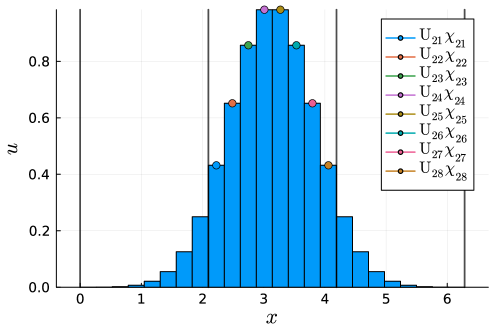
Figure 1: A Gaussian wave discretized by a finite difference scheme represented by a local basis of box functions for $I=3$ subdomains and $J=8$ points per subdomain. The edges of the subdomains are indicated by the vertical grey lines.

After obtaining $\mathbf{U}(t)$ at different points in time the snapshot matrix is constructed as follows

$$\mathbf{X}_{\ell}=\begin{bmatrix}\mathbf{U}^{T}(t_{1})&\mathbf{U}^{T}(t_{2})&\ldots&\mathbf{U}^{T}(t_{s})\end{bmatrix}\quad\in\mathbb{R}^{J\times Is}.$$ (21)

In this way each subdomain is treated equally in the snapshot matrix. This is what differentiates our work from the work in [24], namely the snapshot matrix is built combining all of the subdomains. Using a common snapshot matrix allows us to obtain a space-local POD basis that generalizes well outside the training data. The way we divide the domain in subdomains is decided by what results in an L-POD basis that generalizes best on a validation data set, see section 5.2.

Note that this matrix has fewer rows, but more columns than the G-POD snapshot matrix, see (11). This makes the SVD cheaper to compute for a large number of snapshots $s$ [29]. As in the global case, we use a SVD of the snapshot matrix to obtain a truncated basis $\hat{\boldsymbol{\Gamma}}\in\mathbb{R}^{J\times q}$ with $q<J$ from the left-singular vector. In terms of the local basis $\{\chi_{ij}\}$ the POD basis is written as

$$\gamma_{ij}(x)=\sum^{J}_{k=1}\chi_{ik}(x)\hat{\Gamma}_{kj},$$ (22)

analogous to (18). In this basis the approximated solution $u_{\ell}$ is obtained as

$$u_{h}(x,t)\approx u_{\ell}(x,t)=\sum^{I}_{i=1}\sum^{q}_{j=1}\text{A}_{ij}(t)\gamma_{ij}(x),$$ (23)

similarly to the global case, see (17). The coefficients $\text{A}_{ij}$ are obtained as

$$\mathbf{a}_{\ell}=\boldsymbol{\Gamma}^{T}\mathbf{u},$$ (24)

where

$$\boldsymbol{\Gamma}=\begin{bmatrix}\hat{\boldsymbol{\Gamma}}&&\\ &\ddots&\\ &&\hat{\boldsymbol{\Gamma}}\end{bmatrix}\quad\in\mathbb{R}^{N\times r}.$$ (25)

This matrix, containing non-overlapping blocks, is constructed such that multiplying by its transpose projects $\mathbf{u}$ onto the L-POD basis. For the mapping from $\mathbf{a}_{\ell}\in\mathbb{R}^{Iq}$ to $\mathbf{A}\in\mathbb{R}^{I\times q}$ we follow the same convention as for $\mathbf{u}$ and $\mathbf{U}$. The effective number of basis functions for L-POD is $Iq=r$ with $q<J$. This basis is orthonormal, i.e. $\boldsymbol{\Gamma}^{T}\boldsymbol{\Gamma}=\mathbf{I}$. The sparsity of $\boldsymbol{\Gamma}$, as opposed to $\boldsymbol{\Phi}$, is what yields a ROM which is cheaper to evaluate than a G-POD-based ROM [24].

An example of an L-POD approximation $u_{\ell}$ to a Gaussian wave is shown in Figure 2. For the L-POD we used $I=10$ subdomains with $q=6$ basis functions per subdomain. The training data used to obtain the basis is discussed in the results section (section 5), see Figure 4. Although the L-POD approximation is accurate in most of the domain, some oscillations appear near the boundaries. In addition, the approximation is not guaranteed to be smooth on the edges of the subdomains, see Figure 2. Discontinuities appear when transitioning from one subdomain to the next. In section 5 we will show that these discontinuities tend to grow increasingly severe when using the L-POD basis to construct a ROM, see Figure 7. To remedy this issue, we introduce space-local POD with overlapping subdomains in the next section.

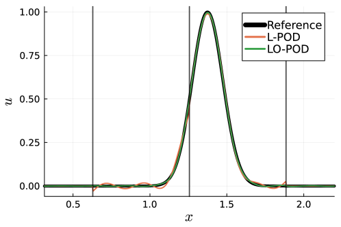
Figure 2: L-POD and LO-POD representation of a Gaussian wave. The data used to obtain the local POD basis is explained in section 5. The depicted snapshot is part of the snapshot matrix used to obtain the POD basis. The edges of the subdomains are indicated by the vertical grey lines. Only part of the domain $\Omega=[0,2\pi)$ is shown.

3.3 Local POD with overlapping subdomains

In finite element discretizations similar discontinuities are resolved by imposing continuity of the approximation, while using a local basis. In this work we aim to achieve the same by introducing a novel space-local POD formulation with overlapping subdomains. We will refer this approach as LO-POD. To start off, we subdivide the domain $\Omega$ into $I$ overlapping subdomains $\Omega_{i}=[\alpha_{i},\beta_{i})$. This means $\beta_{i-2}=\alpha_{i}<\beta_{i-1}=\alpha_{i+1}<\beta_{i}=\alpha_{i+2}$. Once again, each subdomain contains $J$ grid points. Note that due to the overlap each grid point is now located in two subdomains. This means $\frac{I\cdot J}{2}=N$, as opposed to $I\cdot J=N$ for L-POD.

In order to obtain a smooth approximation $u_{\ell}$ we require the LO-POD basis to smoothly decay to zero on the edge of the subdomain. This is enforced through a post-processing step of the local snapshot matrix given by (21). For this purpose we introduce a kernel $k_{i}(x)$ to divide the solution between the subdomains. This places the following constraint on the kernels:

$$\sum^{I}_{i=1}k_{i}(x)=1,$$ (26)

such that this set of functions forms a partition of unity. Here we propose the following kernel

$$k_{i}(x)=\begin{cases}\sin^{2}(\frac{1}{2}\frac{x-\alpha_{i}}{\alpha_{i}-\alpha_{i+1}}\pi)\quad&\text{if }\alpha_{i}\leq x<\alpha_{i+1},\\ \sin^{2}(\frac{1}{2}\frac{x-\alpha_{i+1}}{\alpha_{i+2}-\alpha_{i+1}}\pi+\frac{1}{2}\pi)\quad&\text{if }\alpha_{i+1}\leq x<\alpha_{i+2},\\ 0\quad&\text{elsewhere},\end{cases}$$ (27)

which is chosen as it smoothly decays to zero at the subdomain boundaries. This approach is inspired on the partition of unity method [30]. Here the right half of each subdomain is overlapped by the subdomain on the right and the left half by the subdomain on the left. A visualization of the kernels is displayed in Figure 3.

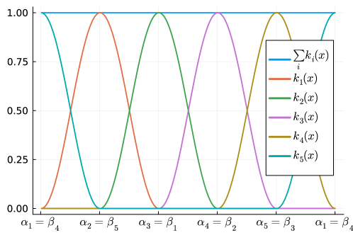
Figure 3: Kernels $k_{i}$ for a subdivision of the periodic domain into five overlapping subdomains of equal size.

Different kernels and different amounts of overlap between subdomains can also be considered. However, we consider this outside the scope of this paper.

Using the introduced kernel, the coefficients $\mathbf{U}$ for the local expansion in (19) are obtained as

$$\text{U}_{ij}(t)=\frac{(\chi_{ij}(x),k_{i}(x)u_{h}(x,t))}{(\chi_{ij}(x),\chi_{ij}(x))}.$$ (28)

These integrals can simply be approximated using the midpoint rule for integration [31]. The remaining procedure stays the same as for L-POD, i.e. we build the snapshot matrix in (21) and carry out a SVD to obtain $\hat{\boldsymbol{\Gamma}}$. However, what changed is that the blocks in $\boldsymbol{\Gamma}$, see (25), are now overlapping. This means the basis is no longer orthonormal, i.e. $\boldsymbol{\Gamma}^{T}\boldsymbol{\Gamma}\neq\mathbf{I}$. Due to the non-orthonormality, the coefficients $\mathbf{a}_{\ell}$ for the expansion in (23) are obtained by solving the following linear system

$$(\boldsymbol{\Gamma}^{T}\boldsymbol{\Gamma})\mathbf{a}_{\ell}=\boldsymbol{\Gamma}^{T}\mathbf{u},$$ (29)

as opposed to (24). This makes obtaining the coefficients from FOM solution more expensive. In addition, evaluating the resulting ROM requires solving a linear system, as discussed in section 4. This makes the LO-POD ROM more expensive to evaluate than its non-overlapping counterpart L-POD, see sections 4.2 and 5.5. However, looking at Figure 2, we find that using the LO-POD results in a much smoother approximation of the Gaussian wave. Note that the parameters are kept the same, i.e. $I=10$ and $q=6$. In section 5.2 the associated error will be quantified more precisely.

4 Space-local, energy-conserving reduced-order model

4.1 Projection on reduced basis

Consider again $\mathbf{c}$, the state vector of the full-order model, and $\boldsymbol{\Phi}\in\mathbb{R}^{N\times r}$ a reduced basis where $r<N$, obtained from either G-POD, L-POD, or LO-POD. For the space-local approaches this operator was referred to as $\boldsymbol{\Gamma}$, see section 3.2. The corresponding ‘Gram’ matrix $\mathbf{S}\in\mathbb{R}^{r\times r}$ of this basis is computed as

$$\mathbf{S}=\boldsymbol{\Phi}^{T}\boldsymbol{\Phi}.$$ (30)

We can project $\mathbf{c}$ onto the subspace spanned by the POD basis as

$$\mathbf{c}_{r}=\underbrace{\boldsymbol{\Phi}\mathbf{S}^{-1}\boldsymbol{\Phi}^{T}}_{=:\mathbf{P}}\mathbf{c}.$$ (31)

Note that for both G-POD and L-POD computing the inverse of $\mathbf{S}$ is trivial, as it is simply identity. This comes from the fact that the basis is orthogonal. However, for LO-POD the basis is non-orthogonal, which makes computing its inverse less trivial. As stated earlier, this is a downside to LO-POD and increases its computational cost. It is quite straightforward to see that $\mathbf{P}$ is a projection operator as $\mathbf{P}^{2}=\mathbf{P}$. The POD coefficient vector is obtained as

$$\mathbf{a}=\mathbf{S}^{-1}\boldsymbol{\Phi}^{T}\mathbf{c}.$$ (32)

4.2 Galerkin projection

Having obtained a reduced basis, we construct a ROM for the advection equation as follows [7, 8, 5, 6]: Based on (6) we define the residual $\mathbf{r}\in\mathbb{R}^{N}$ as

$$\mathbf{r}(\mathbf{u}_{r}):=\frac{\text{d}\mathbf{u}_{r}}{\text{d}t}+c\mathbf{D}\mathbf{u}_{r}\neq\mathbf{0},$$ (33)

where we replaced $\mathbf{u}$ by the POD approximation $\mathbf{u}_{r}=\boldsymbol{\Phi}\mathbf{a}$. As $\mathbf{u}$ comes from the finite difference discretization of the advection equation we have $\mathbf{c}(t)=\mathbf{u}(t)$. Next, we carry out the Galerkin projection of the residual on the POD basis, according to (32), and set this to zero:

$$\mathbf{S}^{-1}\boldsymbol{\Phi}^{T}\mathbf{r}(\mathbf{u}_{r})=\mathbf{0}.$$ (34)

This ensures the residual is orthogonal to the basis. This results in the following ROM:

$$\frac{\text{d}\mathbf{a}^{\text{ROM}}}{\text{d}t}:=-c\mathbf{S}^{-1}\mathbf{A}\mathbf{a}^{\text{ROM}},$$ (35)

where the ROM operator $\mathbf{A}\in\mathbb{R}^{r\times r}$ is defined as

$$\mathbf{A}:=\boldsymbol{\Phi}^{T}\mathbf{D}\boldsymbol{\Phi}.$$ (36)

Note that we introduced $\mathbf{a}^{\text{ROM}}$ here as the POD state vector predicted by ROM. This is typically not equal to the true $\mathbf{a}$, see (32), past $t=0$. Going from the FOM to the ROM we reduced the DOF in the system from $N$ to $r$. In the G-POD case $\mathbf{A}$ is typically dense, whereas in the L-POD/LO-POD it is sparse. The sparsity decreases the cost of evaluating the ROM [24]. The amount of nonzero entries in the G-POD ROM operator scales with $\mathcal{O}(r^{2})$. For L-POD it scales with $\mathcal{O}((3q)^{2}I)$. The prefactor $3$ comes from the interaction with the two neighboring subdomains, in addition to the interaction within the subdomain. For LO-POD two additional subdomains have to included in the interactions due to the overlap. This results in a scaling of $\mathcal{O}((5q)^{2}I)$. For a large number of subdomains $I$ and a small number of POD basis functions per subdomain $q$, with the total number of POD modes being $I\cdot q=r$, this scales more favorably. This allows us to include a larger number of basis functions in the POD basis. For non-linear problems, i.e. Navier-Stokes with the quadratic advection operator the resulting ROM operator is also more sparse [24]. Hyperreduction techniques, including energy-conserving ones, can also be employed to further sparsen the ROM operators [32, 33, 17].

4.3 Energy conservation of the ROM

In order to ensure stability of the ROMs, we aim to mimic the energy conservation property of the FOM. To investigate if the constructed ROMs satisfy this property we define the ROM energy $E_{r}^{\text{ROM}}$ as

$$E_{r}^{\text{ROM}}=\frac{h}{2}(\mathbf{u}_{r}^{\text{ROM}})^{T}(\mathbf{u}_{r}^{\text{ROM}}),$$ (37)

where $\mathbf{u}_{r}^{\text{ROM}}:=\boldsymbol{\Phi}\mathbf{a}^{\text{ROM}}$. Employing (35) we obtain the ROM evolution of $\mathbf{u}_{r}^{\text{\lx@glossaries@gls@link{acronym}{ROM}{\leavevmode ROM}}}$ as

$$\frac{\text{d}\mathbf{u}_{r}^{\text{ROM}}}{\text{d}t}=\boldsymbol{\Phi}\frac{\text{d}\mathbf{a}^{\text{ROM}}}{\text{d}t}=-c\boldsymbol{\Phi}\mathbf{S}^{-1}\mathbf{A}\mathbf{a}^{\text{ROM}}.$$ (38)

The evolution of the ROM energy follows as

$$\begin{split}\frac{\text{d}E_{r}^{\text{ROM}}}{\text{d}t}&=h(\mathbf{u}_{r}^{\text{ROM}})^{T}\frac{\text{d}\mathbf{u}_{r}^{\text{ROM}}}{\text{d}t}=-ch(\mathbf{u}_{r}^{\text{ROM}})^{T}\boldsymbol{\Phi}\mathbf{S}^{-1}\mathbf{A}\mathbf{a}^{\text{ROM}}\\ &=-ch(\mathbf{a}^{\text{ROM}})^{T}\underbrace{\boldsymbol{\Phi}^{T}\boldsymbol{\Phi}}_{=\mathbf{S}}\mathbf{S}^{-1}\boldsymbol{\Phi}^{T}\mathbf{D}\boldsymbol{\Phi}\mathbf{a}^{\text{ROM}}\\ &=-ch(\mathbf{a}^{\text{ROM}})^{T}\boldsymbol{\Phi}^{T}\mathbf{D}\boldsymbol{\Phi}\mathbf{a}^{\text{ROM}}=-ch(\mathbf{u}_{r}^{\text{ROM}})^{T}\mathbf{D}\mathbf{u}_{r}^{\text{ROM}}=0,\end{split}$$ (39)

employing the product rule of differentiation. From the final expression we conclude that a ROM based on Galerkin projection inherits energy conservation and stability from the FOM. This is true for both orthogonal and non-orthogonal projections. This means that not only the G-POD ROM inherits this property, as shown in [9], but also the newly introduced space-local approaches L-POD and LO-POD.

5 Results & discussion

5.1 Test case setup

To construct a ROM we first require data from the FOM. As stated earlier, we use the finite difference discretization of the advection equation, detailed in section 2.2, for this purpose. The system is simulated on a periodic domain $\Omega=[0,2\pi)$ discretized with $N=1000$ grid points for $t=[0,5]$ and constant $c=1$. A time step size of $\Delta t=0.01$ is used for the time integration, using a RK4 scheme. This is the largest time step size which still yielded stable simulations. Snapshot data for the ROM construction is collected in the interval $t=[0,1]$. We refer to this as the training data. Data generated in the interval $t=(1,2]$ will be referred to as validation data. This data is used to evaluate the generalization of the POD basis. The remaining part of the simulation data, $t=(2,5]$, will be used to evaluate the extrapolation capabilities of the ROMs. As an initial condition we use a Gaussian wave centred around $x=\frac{1}{4}\pi$, namely

$$u(x,0)=\exp(-50(x-\frac{1}{4}\pi)^{2}).$$ (40)

A visualization of this simulation is displayed in Figure 4.

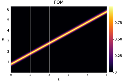
Figure 4: Reference simulation of a Gaussian wave being advected throughout the domain. White bars separate training data from validation data and validation data from extrapolation data, respectively.

For the ROMs we consider the three bases discussed in this work: the global POD basis G-POD, the space-local POD basis L-POD, and the space-local POD basis with overlapping subdomains LO-POD. For the space-local approaches the domain is subdivided into $I$ subdomains. For the local basis $\{\chi_{ij}\}$ we use $J$ box functions contained within each subdomain, such that $IJ=N$. In this way the local basis aligns with the FOM finite difference basis, see (10). The integrals in the LO-POD post-processing step, equation (28), are approximated using the midpoint rule for integration [31]. For the ROM time integration we use the same RK4 scheme as for the FOM.

To evaluate the ROMs we evaluate the difference between the ROM solution $\mathbf{u}^{\text{ROM}}:=\boldsymbol{\Phi}\mathbf{a}^{\text{ROM}}$ and the FOM solution $\mathbf{u}^{\text{FOM}}$:

$$\underbrace{\mathbf{u}^{\text{ROM}}_{r}(t)-\mathbf{u}^{\text{FOM}}(t)}_{:=\text{solution error}}=\underbrace{\mathbf{u}_{r}^{\text{ROM}}(t)-\mathbf{P}\mathbf{u}^{\text{FOM}}(t)}_{:=\text{ROM error}}+\underbrace{\mathbf{P}\mathbf{u}^{\text{FOM}}(t)-\mathbf{u}^{\text{FOM}}(t)}_{:=\text{projection error}},$$ (41)

where $\mathbf{P}$ projects the solution on the POD basis, see (31). This difference will be referred to as the solution error. In (41) this error is decomposed as the the sum of the ROM error (the error made by the ROM during the time integration) and the projection error (the error made by the reduced basis approximation). Our implementation, in Julia [34], of the introduced methodologies and experiments are freely available on Github, see https://github.com/tobyvg/local_POD_overlap.jl.

5.2 Projection error

For the construction of the L-POD and LO-POD ROMs we have to determine the number of subdomains $I$ and the number of modes per subdomain $q$, with $Iq=r$, which results in a basis that generalizes best outside the training data. To do this we evaluate the projection error, see (41), on both the training and validation data. The results are depicted in Figure 5 for different $I$, averaged over both the training (solid line) and validation data (dashed line).

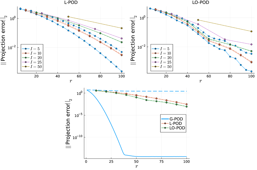
Figure 5: (Top) Projection error evaluated over the training (solid line) and validation (dashed line) data for different $I$. (Bottom) Projection error for $I=10$ for L-POD and LO-POD evaluated over the training (solid line) and validation (dashed line) data. The projection error for G-POD is also depicted.

A basis that generalizes well should perform well on both the training and validation data. We observe that for $I=5$ the training error is lowest, but the validation error is rather large, so the basis does not generalize well. For higher values of $I$, the training and validation errors are much closer, but tend to increase with increasing $I$. In this case, $I=10$ is considered optimal as the training and validation error are small and similar in size. This is true for both L-POD and LO-POD. For the remainder of this text we will therefore stick to $I=10$ for the construction of the local ROMs. In general, the choice for $I$ is likely problem dependent and an a-priori study similar to Figure 5 needs to be performed to choose an optimal value.

Next, we compare the performance of the space-local approaches against each other, as well as to G-POD. This is also displayed in Figure 5 (bottom plot). We observe that the projection error converges faster for LO-POD, as compared to L-POD. This can be explained by the fact the LO-POD basis functions are constructed from twice as many finite difference points as for L-POD, due to the overlapping subdomains. This means there are twice as many DOF fit in the POD procedure, which yields a lower projection error. The difference between convergence on the training and validation data is small for both space-local approaches. On the other hand, for G-POD the convergence of the projection error on the training data is very fast, see (13), but on the validation data the error hardly converges. This is because the G-POD is only suited for representing the wave in the left side of the domain, as detailed in the next section. We conclude that the space-local approaches result in a basis that generalizes better than the global approach, for this particular problem.

5.3 Resulting basis

The resulting local basis functions for $q=6$ are displayed in Figure 6 along with the first six G-POD modes.

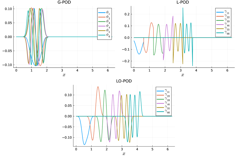
Figure 6: The first six G-POD modes and the first six space-local POD modes for L-POD and LO-POD. For visualization purposes the space-local POD modes are displayed on adjacent subdomains.

We find that the G-POD modes are only nonzero where the traveling wave is represented in the training data. This explains the fact that the error on the validation data hardly converged in Figure 5. For the space-local approaches, where a common basis is ”copy/pasted” across the entire domain, this is not an issue. Regarding L-POD we observe that the obtained basis functions do not smoothly decay to zero at the edge of the subdomain, but instead end abruptly. Finally, we observe that for LO-POD the post-processing procedure in (28) indeed results in a basis that smoothly decays on the edge of the subdomains.

5.4 Accuracy and energy conservation of ROMs

Having obtained a basis for each of the POD approaches we construct a set of ROMs. Based on the results in section 5.2 we select $r=60$, $I=10$, and $q=6$ for the space-local approaches. To keep the size of the basis the same we select $r=60$ for G-POD. The ROM results are obtained by evaluating (35) from the initial condition in (40). The resulting simulations up to $t=5$ are presented in Figure 7.

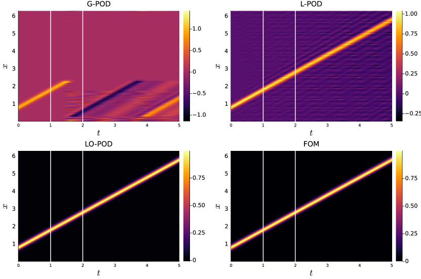
Figure 7: Trajectories of $\mathbf{u}_{r}$ for the different ROMs, along with the FOM trajectory. From left to right, the white lines indicate the end of the training data and validation data, respectively.

For G-POD we find that after the training data the performance degrades significantly. This exposes the limitations of G-POD, as it is not able to adapt to the wave traveling outside the training range. The space-local approaches perform better in this regard. Both L-POD and LO-POD are capable of extrapolating the traveling of the wave past the training region. However, L-POD seems to suffer from discontinuities in $\mathbf{u}_{r}^{\text{ROM}}$, as the edges of the subdomains become increasingly visible as the simulation progresses. LO-POD does not suffer from this issue and smoothly extrapolates the solution past the training region. This means the smooth reconstruction coming from LO-POD indeed improves the quality of the simulation for the same number of DOF.

Next, we evaluate the ROMs on a set of performance metrics. The first metric is the solution error, see (41). The other metrics (defined on the figure axes) focus on how well the energy is conserved during the simulation, namely the total change in energy and the instantaneous change in energy. The results are shown in Figure 8.

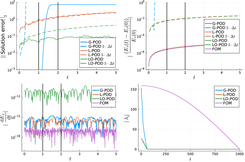
Figure 8: (Top-left) Solution error for each of ROMs during the simulation, presented for both $\Delta t=0.01$ and $\Delta t=0.05$. From left to right, the black lines indicate the end of the training data and validation data, respectively. (Top-right) Relative change in energy with respect to the start of the simulation. (Bottom-left) Instantaneous change in energy, computed by evaluating (39). (Bottom-right) Eigenvalues of the projected FOM operator.

The results are depicted for both the FOM time step size $\Delta t$ (solid line) and a five times larger time step $5\cdot\Delta t$ (dashed line). This larger time step is based on an eigenvalue analysis of the ROM operator, also presented in Figure 8. For this analysis we determined the eigenvalues of the operator $\mathbf{D}$ projected on the ROM basis. This operator is given by $\mathbf{P}\mathbf{D}\mathbf{P}$. It can be shown that replacing $\mathbf{D}$ in the FOM, see (6), by this projected operator is equivalent to integrating the ROM, see (35). The eigenvalues $\lambda_{i}$ are ordered according to the magnitude of their absolute values. We observe that the largest eigenvalue for the space-local approaches is roughly five times smaller than the one of G-POD and the FOM. This is likely caused by the fact that the G-POD basis functions contain higher frequencies than the space-local basis functions, see Figure 6. Using a smaller G-POD basis could alleviate this. Based on this analysis we also evaluate the performance of the ROMs for a five times larger time step [35].

Looking at the solution error we observe that G-POD performs best in the training region (the error is so small that it is outside the plotting range). However, after leaving the training region ($t>1$) the performance degrades rapidly. On the other hand, for the space-local approaches we do not observe this jump of error outside the training region, but rather a steady increase. Importantly, outside the training region the space-local approaches are much more accurate than G-POD. In particular acrshortLO-POD improves with more than one order of magnitude upon both G-POD and L-POD outside the training region.

When increasing the size of the time step by five-fold the simulation quickly becomes unstable for G-POD. For L-POD both time steps yield stable simulations, giving results that are very close to each other. For LO-POD and a smaller time step size the error seems to converge to an equilibrium. However, for a larger time step it increases steadily. This means there is likely still a benefit to taking a smaller time step. An interesting continuation of this research would be to find a way to systematically determine the ”sweet spot” between increasing the time step and maintaining accuracy of the ROM.

In terms of energy conservation, we observe that all ROMs conserve the energy as predicted by the theoretical analysis, except for a time discretization error incurred by the use of RK4. This error increases when the time step size is increased. Only for G-POD with an increased time step size the simulation becomes unstable. For LO-POD the numerical error in the instantaneous change in energy, see (39), is the largest. This is likely due the linear system that needs to be solved to evaluate the ROM for a non-orthogonal basis, see (35). However, the time discretization error seems to be the main source of error, as the change in energy during the simulation is roughly the same for L-POD and LO-POD.

5.5 Convergence with increasing ROM dimension

Finally, we look at the convergence of the solution error as we increase the size of ROM basis $r$. In addition, we compare the ROMs to a finite difference discretization with the same number of DOF. Note that for the ROMs $\text{DOF}=r$. For the finite difference simulations we first project the solution on the FOM grid using linear interpolation. We then compute the difference, such as in (41), and compute the $L_{2}$-norm to quantify the error. For the local ROMs we stick to $I=10$ subdomains, while increasing the number of basis functions per subdomain $q$ to increase $r$. We consider a maximum of $r=100$ for the ROMs.

The results are depicted in Figure 9.

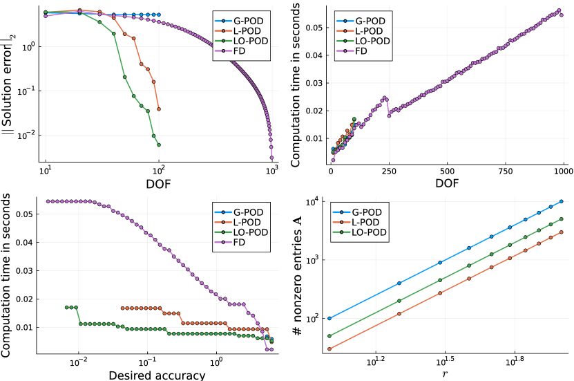
Figure 9: (Top-left) Solution error averaged over a simulation up to $t=5$. Results are presented for the different ROMs, as well as a finite difference discretization (FD) with the same number of DOF. (Top-right) Computation time required to carry out the simulation for each number of DOF. Depicted computation times represent an average of 10 duplicate simulations. (Bottom-left) Computation time required to achieve a certain level of accuracy in the solution error for the different ROMs and the finite difference discretization. (Bottom-right) Number of nonzero entries in the ROM operator $\mathbf{A}$.

Regarding the local ROMs we observe rapid convergence of the solution error as we increase the number of DOF, with LO-POD consistently outperforming L-POD. This is in line with the projection error convergence discussed in section 5.2. Regarding G-POD we observe no convergence of the solution error. Regarding the finite difference discretization we find it converges at a much slower rate than the space-local ROMs.

In Figure 9 we also consider the required computation time for each number of DOF. For this purpose we evaluated our code on a laptop CPU. The ROMs were implemented in Julia using sparse matrices [34]. For both the ROMs and the finite difference discretization we use the FOM time step size, for ease of comparison. We observe that the computation time of the ROMs scales similarly to the FOM with respect to the number of DOF (roughly linear). For larger systems the results may vary, as evaluating the LO-POD ROM requires solving a linear system because of the non-orthogonal basis. Solving general linear systems scales at most cubically with the number of DOF [36]. In this case we simply precomputed the inverse of matrix $\mathbf{S}$ and evaluated the LO-POD ROM using dense matrix-vector multiplication. In future work the sparsity, symmetry, and positive-definiteness matrix can possible be employed to speed up this procedure [37]. However, for this small system dense-matrix vector multiplication turned out to be the most efficient. Evaluating the G-POD scales quadratically with the number of DOF, as the ROM operator $\mathbf{A}$ is typically dense for a G-POD basis [24]. For L-POD evaluating the ROM scales the most favorable as $\mathbf{A}$ is sparse and one does not need to solve a linear system. Evaluating the L-POD is therefore likely the cheapest option for larger systems. However, for the size of the problem we consider the computational cost is likely dominated by computational overhead.

Next, we look at the required computation time needed to reach a certain level of accuracy. Here we find that both local ROMs, and especially LO-POD, can achieve a desired accuracy at a much lower computational time. Both space-local ROMs significantly outperform the finite difference discretization. One thing to note is that in order to generate the ROM one first needs to generate the training data, carry out the POD, and construct the ROM operator. This was not included in the recorded computation time. However, when carrying out multiple simulations, such as done in optimization procedures, the time spend on these precomputations quickly becomes negligible [1]. We therefore decided not to add this to the presented computation times.

To obtain a conclusive answer about the scaling of the ROMs we considered the number of nonzero entries in the ROM operator $\mathbf{A}$. This is also depicted in Figure 9. Here we find that the number of nonzero entries scales according to a power law, with L-POD scaling the most favorably. This is in line with the discussion presented in section 4.2. Hyperreduction can be carried out to further reduce the computational cost of the ROMs [32, 33, 17]. Finally, one could also increase the time step size, as discussed in section 5.4, to further decrease the computational cost of the space-local ROMs.

6 Conclusions

In this work, we presented a novel way of constructing ROMs for PDE describing advection-dominated problems. The key properties of our proposed ROM are: sparsity and generalizability through a space-local ROM with overlapping subdomains; stability by embedding energy conservation in the ROM. The space-local ROMs are achieved by building a POD basis within each subdomain, as compared to a single common basis for the standard space-global approach. In [24] it was shown that such a basis results in a sparse and computationally efficient ROM. We modified this approach to generate a common local basis for the entire domain, similarly to a finite element basis. By generating a common basis we achieve generalizability, as in this way a feature observed in one subdomain can now be represented in any of the subdomains. To introduce our methodology we made use of the linear advection equation. One of the properties of this is system that the energy is conserved. As full-order model (FOM) we therefore use an energy conserving central difference scheme.

We observed that the resulting space-local ROMs generalize much better for advection-dominated problems than the standard space-global approach. In addition, we showed that the space-local ROMs also satisfy energy conservation and allow for larger time steps. The latter further decreases the computational cost of the ROMs. Regarding the computational time, we observed an improvement of roughly five-fold with respect to the full-order model (FOM), depending on the required accuracy. By taking a large time step size for the space-local ROMs we could achieve an additional speedup of roughly five-fold. Furthermore, we showed increased sparsity of the ROM operator for the space-local approaches with respect to the space-global approach. However, for the small system considered here this did not result in a computational speedup with respect to the ROM constructed from a space-global basis.

For future research, we consider the extension of this methodology to an actual turbulence test case described by the Navier-Stokes equations. A starting point would be the work presented in [24]. To achieve energy-conservation one can make use of the observation presented in [9], where it was shown that carrying out a Galerkin projection on an energy-conserving FOM (with quadratic non-linearity) resulted in an energy-conserving ROM. However, one important requirement is that the POD basis needs to be divergence free, meaning that the space-local POD basis also needs to be divergence free. Currently, this is still being actively researched in our group. In addition, one could consider reusing the learned space-local basis for different spatial domains than represented in the training data. Another possible research direction would be to circumvent or speed up the solution of the linear system required in LO-POD. For this purpose, one could possibly take inspiration from the finite element community [25].

Glossary

Acronyms

DOF

degrees of freedom

FOM

full-order model

G-POD

global proper orthogonal decomposition

L-POD

space-local proper orthogonal decomposition

LO-POD

space-local proper orthogonal decomposition with overlapping subdomains

LSTM

long short-term memory

PDE

partial differential equation

POD

proper orthogonal decomposition

RK4

Runge-Kutta 4

ROM

reduced-order model

Declarations

Data & code availability

The code used to generate the training data, construct the ROMs, and replicate the presented experiments can found at https://github.com/tobyvg/local_POD_overlap.jl.

Competing interests

The authors declare that they have no competing interests.

Funding

This publication is part of the project “Unraveling Neural Networks with Structure-Preserving Computing” (with project number OCENW.GROOT.2019.044 of the research programme NWO XL which is financed by the Dutch Research Council (NWO)). Part of this publication is funded by Eindhoven University of Technology.

Authors’ contributions

T. van Gastelen: Conceptualization, Methodology, Software, Writing - original draft. W. Edeling: Writing - review & editing. B. Sanderse: Conceptualization, Methodology, Writing - review & editing, Funding acquisition.

References

- \bibcommenthead
- Sasaki et al. [2002] Sasaki, D., Obayashi, S., Nakahashi, K.: Navier-stokes optimization of supersonic wings with four objectives using evolutionary algorithm. Journal of Aircraft 39(4), 621–629 (2002)
- Agdestein and Sanderse [2024] Agdestein, S.D., Sanderse, B.: Discretize first, filter next: learning divergence-consistent closure models for large-eddy simulation (2024). https://arxiv.org/abs/2403.18088
- Alfonsi [2009] Alfonsi, G.: Reynolds-averaged navier-stokes equations for turbulence modeling. Applied Mechanics Reviews - APPL MECH REV 62 (2009) https://doi.org/10.1115/1.3124648
- Sagaut and Lee [2002] Sagaut, P., Lee, Y.-T.: Large eddy simulation for incompressible flows: An introduction. scientific computation series. Applied Mechanics Reviews 55, 115 (2002) https://doi.org/10.1115/1.1508154
- Brunton and Kutz [2019] Brunton, S.L., Kutz, J.N.: Data-Driven Science and Engineering: Machine Learning, Dynamical Systems, and Control, 1st edn. Cambridge University Press, USA (2019)
- Benner et al. [2015] Benner, P., Gugercin, S., Willcox, K.: A survey of projection-based model reduction methods for parametric dynamical systems. SIAM Review 57(4), 483–531 (2015) https://doi.org/10.1137/130932715 https://doi.org/10.1137/130932715
- Burkardt et al. [2006] Burkardt, J., Gunzburger, M., Lee, H.-C.: Pod and cvt-based reduced-order modeling of navier–stokes flows. Computer Methods in Applied Mechanics and Engineering 196, 337–355 (2006) https://doi.org/10.1016/j.cma.2006.04.004
- Rapun and Vega [2010] Rapun, M.-L., Vega, J.: Reduced order models based on local pod plus galerkin projection. Journal of Computational Physics 229 (2010) https://doi.org/%****␣sn-article.bbl␣Line␣150␣****10.1016/j.jcp.2009.12.029
- Sanderse [2020] Sanderse, B.: Non-linearly stable reduced-order models for incompressible flow with energy-conserving finite volume methods. Journal of Computational Physics 421, 109736 (2020) https://doi.org/10.1016/j.jcp.2020.109736
- Dutta et al. [2022] Dutta, S., Rivera-Casillas, P., Styles, B., Farthing, M.W.: Reduced order modeling using advection-aware autoencoders. Mathematical and Computational Applications 27(3) (2022) https://doi.org/10.3390/mca27030034
- Arbes et al. [2024] Arbes, F., Greif, C., Urban, K.: The Kolmogorov N-width for linear transport: Exact representation and the influence of the data (2024). https://arxiv.org/abs/2305.00066
- Taddei et al. [2015] Taddei, T., Perotto, S., Quarteroni, A.: Reduced basis techniques for nonlinear conservation laws. ESAIM: Mathematical Modelling and Numerical Analysis 49(3), 787–814 (2015)
- Greif and Urban [2019] Greif, C., Urban, K.: Decay of the kolmogorov n-width for wave problems. Applied Mathematics Letters 96, 216–222 (2019)
- Carlberg et al. [2013] Carlberg, K., Farhat, C., Cortial, J., Amsallem, D.: The gnat method for nonlinear model reduction: effective implementation and application to computational fluid dynamics and turbulent flows. Journal of Computational Physics 242, 623–647 (2013)
- Nair and Balajewicz [2019] Nair, N.J., Balajewicz, M.: Transported snapshot model order reduction approach for parametric, steady-state fluid flows containing parameter-dependent shocks. International Journal for Numerical Methods in Engineering 117(12), 1234–1262 (2019)
- Washabaugh et al. [2012] Washabaugh, K., Amsallem, D., Zahr, M., Farhat, C.: Nonlinear model reduction for cfd problems using local reduced order bases. (2012). https://doi.org/10.2514/6.2012-2686
- Klein and Sanderse [2024] Klein, R.B., Sanderse, B.: Energy-conserving hyper-reduction and temporal localization for reduced order models of the incompressible navier-stokes equations. Journal of Computational Physics 499, 112697 (2024) https://doi.org/10.1016/j.jcp.2023.112697
- Peherstorfer and Willcox [2015] Peherstorfer, B., Willcox, K.: Online adaptive model reduction for nonlinear systems via low-rank updates. SIAM Journal on Scientific Computing 37(4), 2123–2150 (2015) https://doi.org/10.1137/140989169 https://doi.org/10.1137/140989169
- Grimberg et al. [2020] Grimberg, S., Farhat, C., Youkilis, N.: On the stability of projection-based model order reduction for convection-dominated laminar and turbulent flows. Journal of Computational Physics 419, 109681 (2020) https://doi.org/10.1016/j.jcp.2020.109681
- Wang et al. [2012] Wang, Z., Akhtar, I., Borggaard, J., Iliescu, T.: Proper orthogonal decomposition closure models for turbulent flows: A numerical comparison. Computer Methods in Applied Mechanics and Engineering 237-240, 10–26 (2012) https://doi.org/10.1016/j.cma.2012.04.015
- Klein et al. [2024] Klein, R., Sanderse, B., Costa, P., Pecnik, R., Henkes, R.: Entropy-Stable Model Reduction of One-Dimensional Hyperbolic Systems using Rational Quadratic Manifolds (2024). https://arxiv.org/abs/2407.12627
- Mohan and Gaitonde [2018] Mohan, A.T., Gaitonde, D.V.: A Deep Learning based Approach to Reduced Order Modeling for Turbulent Flow Control using LSTM Neural Networks (2018). https://arxiv.org/abs/1804.09269
- Mücke et al. [2021] Mücke, N.T., Bohté, S.M., Oosterlee, C.W.: Reduced order modeling for parameterized time-dependent pdes using spatially and memory aware deep learning. Journal of Computational Science 53, 101408 (2021) https://doi.org/10.1016/j.jocs.2021.101408
- Anderson et al. [2022] Anderson, S., White, T., Farhat, C.: Space‐local reduced‐order bases for accelerating reduced‐order models through sparsity. International Journal for Numerical Methods in Engineering 124 (2022) https://doi.org/10.1002/nme.7179
- Reddy [2019] Reddy, J.N.: Introduction to the Finite Element Method, 4th edition edn. McGraw-Hill Education, New York (2019). https://www.accessengineeringlibrary.com/content/book/9781259861901
- Butcher [2007] Butcher, J.: Runge-Kutta methods. Scholarpedia 2(9), 3147 (2007) https://doi.org/10.4249/scholarpedia.3147 . revision #91735
- Sanderse [2013] Sanderse, B.: Energy-conserving runge–kutta methods for the incompressible navier–stokes equations. Journal of Computational Physics 233, 100–131 (2013) https://doi.org/10.1016/j.jcp.2012.07.039
- Aiken et al. [1980] Aiken, J.G., Erdos, J.A., Goldstein, J.A.: On löwdin orthogonalization. International Journal of Quantum Chemistry 18(4), 1101–1108 (1980)
- Li et al. [2019] Li, X., Wang, S., Cai, Y.: Tutorial: Complexity analysis of Singular Value Decomposition and its variants (2019). https://arxiv.org/abs/1906.12085
- Melenk and Babuška [1996] Melenk, J.M., Babuška, I.: The partition of unity finite element method: Basic theory and applications. Computer Methods in Applied Mechanics and Engineering 139(1), 289–314 (1996) https://doi.org/10.1016/S0045-7825(96)01087-0
- Dragomir et al. [1998] Dragomir, S.S., Cerone, P., Sofo, A.: Some remarks on the midpoint rule in numerical integration. RGMIA research report collection 1(2) (1998)
- Ştefănescu and Navon [2013] Ştefănescu, R., Navon, I.M.: Pod/deim nonlinear model order reduction of an adi implicit shallow water equations model. Journal of Computational Physics 237, 95–114 (2013)
- Nguyen et al. [2020] Nguyen, V.B., Tran, S.B.Q., Khan, S.A., Rong, J., Lou, J.: Pod-deim model order reduction technique for model predictive control in continuous chemical processing. Computers & Chemical Engineering 133, 106638 (2020) https://doi.org/10.1016/j.compchemeng.2019.106638
- Bezanson et al. [2017] Bezanson, J., Edelman, A., Karpinski, S., Shah, V.B.: Julia: A fresh approach to numerical computing. SIAM Review 59(1), 65–98 (2017) https://doi.org/10.1137/141000671
- Baldauf [2008] Baldauf, M.: Stability analysis for linear discretisations of the advection equation with runge–kutta time integration. Journal of Computational Physics 227(13), 6638–6659 (2008) https://doi.org/10.1016/j.jcp.2008.03.025
- Bojańczyk [1984] Bojańczyk, A.: Complexity of solving linear systems in different models of computation. SIAM Journal on Numerical Analysis 21(3), 591–603 (1984) https://doi.org/10.1137/0721041 https://doi.org/10.1137/0721041
- Nikishin and Yeremin [1995] Nikishin, A.A., Yeremin, A.Y.: Variable block cg algorithms for solving large sparse symmetric positive definite linear systems on parallel computers, i: General iterative scheme. SIAM journal on matrix analysis and applications 16(4), 1135–1153 (1995)